Particle Dynamics for Learning EBMs

Abstract

Energy-based modeling is a promising approach to unsupervised learning, which yields many downstream applications from a single model. The main difficulty in learning energy-based models with the “contrastive approaches” is the generation of samples from the current energy function at each iteration. Many advances have been made to accomplish this subroutine cheaply. Nevertheless, all such sampling paradigms run MCMC targeting the current model, which requires infinitely long chains to generate samples from the true energy distribution and is problematic in practice. This paper proposes an alternative approach to getting these samples and avoiding crude MCMC sampling from the current model. We accomplish this by viewing the evolution of the modeling distribution as (i) the evolution of the energy function, and (ii) the evolution of the samples from this distribution along some vector field. We subsequently derive this time-dependent vector field such that the particles following this field are approximately distributed as the current density model. Thereby we match the evolution of the particles with the evolution of the energy function prescribed by the learning procedure. Importantly, unlike Monte Carlo sampling, our method targets to match the current distribution in a finite time. Finally, we demonstrate its effectiveness empirically comparing to MCMC-based learning methods.

1 Introduction

Energy-based modeling has recommended itself as a universal approach learning a single model, which then can be applied in various scenarios: continual learning, missing data imputation, out-of-distribution detection, better uncertainty of discriminative models (Grathwohl et al., 2019; Du & Mordatch, 2019; Li et al., 2020). However, scaling this approach to real-world data such as images encounters many complications, which the community has been approaching by trying to get better samples (Tieleman & Hinton, 2009; Du & Mordatch, 2019; Nijkamp et al., 2019) or by targeting different objectives (Grathwohl et al., 2020; Arbel et al., 2020; Gao et al., 2020).

In this paper, we approach the subroutine problem of getting samples from the current model, which arises in the learning of the energy-based models. The conventional approach to this is to run an MCMC method targeting the current model. Instead, we update particles deterministically propagating them along the derived vector field such that after time $dt$ the particles are distributed as the evolved density after time $dt$. This is principally different, since we don’t rely on the convergence to the target (the current model density), and are able to match it in a finite amount of time. Our main contribution is the formula (8) for the vector field, which matches the evolution of the model with the evolution of the particles in the space of log-densities. Further, we discuss possible ways to simulate this formula and demonstrate its usefulness empirically.

2 Background and Related Works

Energy-Based Models are usually learned via the maximum likelihood principle. That is, we start with a model density function $q(x)$ parameterized by the energy function $E(x,\theta)$:

$$q_{\theta}(x)=\frac{1}{Z}e^{-E(x,\theta)},\;\;\;Z=\int dx\;e^{-E(x,\theta)},$$ (1)

which is then optimized to approximate some target density $p(x)$ given empirically (as a set of samples). This can be done by the maximization of $\mathbb{E}_{p}\log q$, or, equivalently, minimization of ${\mathrm{KL}}(p,q)$ via the gradient methods:

$$-\nabla_{\theta}{\mathrm{KL}}(p,q_{\theta})=-\nabla_{\theta}\bigg{[}\mathbb{E}_{x\sim p}E(x,\theta)-\mathbb{E}_{x\sim q_{\theta}}E(x,\theta)\bigg{]},$$ (2)

The main obstacle under this approach is the sampling from the current density $q_{\theta}\propto\exp(-E(x,\theta))$. Our work operates much in the fashion of the Persistent Contrastive Divergence (PCD) (Tieleman & Hinton, 2009). It keeps a set of samples, which are updated at every iterations to match current $q_{\theta}$. While PCD relies on MCMC methods targeting $q_{\theta}$, we propagate the particles deterministically along the derived vector field.

Langevin Dynamics is a ubiquitous sampling method. For energy-based models with the continuous state-space, this method is especially attractive due to its cheap iterations (single gradient evaluation per step) and the ability to yield good samples even without Metropolis-Hastings correction (Gelfand & Mitter, 1991). This procedure targeting the density $p$ can be written as

$$x_{t+dt}=x_{t}+dt\frac{1}{2}\nabla_{x}\log p(x)+\varepsilon,\;\;\;\varepsilon\sim\mathcal{N}(0,dt)$$ (3)

Its efficiency, however, is hindered by the random fluctuations that introduce random-walk behaviour, and its deterministic analog is more efficient (see, for instance, (Liu et al., 2019)). This analog is derived by rewriting the Fokker-Planck equation (which describes the evolution of the density) as the continuity equation:

$$\frac{\partial q}{\partial t}=-\langle\nabla,q\frac{1}{2}\nabla\log p\rangle+\frac{1}{2}\Delta q=-\bigg{\langle}\nabla,q(\frac{1}{2}\nabla\log p-\frac{1}{2}\nabla\log q)\bigg{\rangle}.$$ (4)

Then the simulation of the particles can be done by propagating them along the new vector field:

$$x_{t+dt}=x_{t}+\frac{dt}{2}\big{[}\nabla\log p(x_{t})-\nabla\log q_{t}(x_{t})\big{]}.$$ (5)

In Monte Carlo setting, the deterministic simulation is troublesome since we don’t have an access to the current density $q_{t}$. However, we will see how the EBMs learning naturally allows for this.

3 Matching the particle dynamics with the energy evolution

In this section, we try to match two things: the update of the energy and the update of the particles. The former is defined by the learning procedure maximizing the log-likelihood. The particles then should be propagated to keep up with the updates of energy and be distributed as the most recent model. We match these two dynamics by matching the updates of their log-densities in $L_{q}^{2}$:

$$v^{*}=\operatorname*{max\cdot arg\,max}_{v\in L^{2}_{q}:\left\lVert v\right\rVert=1}\bigg{\langle}\frac{\partial}{\partial t}\log q_{t},\frac{\partial}{\partial t}\log\hat{q}_{t}\bigg{\rangle}_{L_{q}^{2}},$$ (6)

where “$\operatorname*{max\cdot arg\,max}$” denotes the scalar multiplication of the maximum and the maximizer, $q_{t}$ is the prescribed evolution, and $\hat{q}_{t}$ is the density evolution of particles defined by the vector field $v$, i.e.

$$\frac{\partial}{\partial t}\log\hat{q}_{t}=\frac{1}{\hat{q}_{t}}\frac{\partial\hat{q}_{t}}{\partial t}=-\langle\nabla\log q_{t},v\rangle-\langle\nabla,v\rangle.$$ (7)

Proposition 1.

For the evolution of the density $q_{t}=\exp(-E_{t})/Z_{t}$, the solution of equation (6) is

$$v^{*}=-\nabla\frac{\partial E_{t}}{\partial t}.$$ (8)

(See proof in Appendix A). This formula is the main development of our work and in the next section we discuss its practical implications. In a similar way, we can project the evolution of the density

$$v^{\star}=\operatorname*{max\cdot arg\,max}_{v\in L^{2}_{q}:\left\lVert v\right\rVert=1}\big{\langle}\dot{q},-\langle\nabla,qv\rangle\big{\rangle}_{L^{2}}=\operatorname*{max\cdot arg\,max}_{v\in L^{2}_{q}:\left\lVert v\right\rVert=1}\big{\langle}\nabla\dot{q},v\big{\rangle}_{L^{2}_{q}}=\nabla\dot{q},$$ (9)

which is related to the gradient flows in the Wasserstein Riemannian manifold (Otto, 2001; Benamou & Brenier, 2000). These two vector fields are equivalent when the distribution follows the gradient of some functional $F$.

Proposition 2.

Consider the functional $F=\int f(q)$, which we can optimize either w.r.t. $q=\exp(-E)/Z$ or w.r.t. $E$. When the evolution of the density (energy) is defined by the Frechet derivatve of $F$, we have $v^{*}=v^{\star}$.

(See proof in Appendix B). This preposition gives us a reasonable result. Namely, the dynamics of the particles is independent of the distribution parameterization when the parameterization is dense in the corresponding spaces.

Another motivation for the derived formula is that it can be approximated by the Persistent Contrastive Divergence with the Langevin dynamics.

Proposition 3.

The updates of the particles following $v^{*}=-\nabla\frac{\partial E}{\partial t}$ can be approximated as

$$x_{t+dt}=x_{t}-\nabla_{x_{t}}E_{t+dt}(x_{t})+\sqrt{2}\varepsilon,\;\;\;\varepsilon\sim\mathcal{N}(0,1).$$ (10)

(See derivations in Appendix C). In the following section, we will see that the derived formula $v^{*}=-\partial E/\partial t$ allows for different approximations, which avoid any stochasticity in the updates.

4 Numeric approximations of the particle dynamics

First, we consider the approximations that follow straightforwardly by discretizing formula (8). Discretizing the energy update, we have

$$v^{*}(x)=-\nabla_{x}\frac{\partial E_{t}(x)}{\partial t}\approx\frac{1}{dt}\bigg{[}-\nabla(E_{t+dt}(x)-E_{t}(x))\bigg{]}=v_{\alpha}(x).$$ (11)

The update of each individual particle can be written as

$$x_{t+dt}\approx x_{t}+dt\cdot v_{\alpha}(x_{t})=x_{t}-\nabla_{x_{t}}E(x_{t},\theta(t+dt))+\nabla_{x_{t}}E_{t}(x_{t},\theta(t)),$$ (12)

We denote this update rule Method $\bm{\alpha}$. This method is basically the simulation of the Langevin dynamics, but in a deterministic way. Indeed, taking $p(\cdot)\propto\exp(-E(\cdot,\theta(t+dt))$ in equation (5), we obtain the same formula up to the choice of the step-size. Intuitively, this procedure tries to match the new log-density following its gradient and, at the same time, unmatch the old log-density. We describe the full training procedure in Algorithm 1.

The second option, for the parametric models, is to discretize the update of parameters instead:

$$v^{*}= -\nabla\frac{\partial E}{\partial t}=-\nabla\bigg{\langle}\nabla_{\theta}E(\cdot,\theta),\frac{\partial\theta}{\partial t}\bigg{\rangle}\approx-\frac{1}{dt}\nabla\bigg{\langle}\nabla_{\theta}E(\cdot,\theta(t)),\theta(t+dt)-\theta(t)\bigg{\rangle}=v_{\beta}.$$ (13)

This formula gives us another update rule, which we call Method $\bm{\beta}$:

$$x_{t+dt}\approx x_{t}+dt\cdot v_{\beta}(x_{t})=x_{t}-\nabla_{x_{t}}\langle\nabla_{\theta}E(x_{t},\theta(t)),\theta(t+dt)-\theta(t)\rangle.$$ (14)

Unlike method $\alpha$, this method is different from deterministic Langevin, and we will return to its intuition in a bit. For the full training procedure, see Algorithm 1.

Algorithm 1 Methods $\alpha,\beta$

0:  samples from the target distribution $p(x)$

  get initial samples $\{x^{(i)}_{0}\}_{i=1}^{n}\sim q_{\theta(0)}(x)\propto\exp(-E(x,\theta(0)))$

  for $t\in[0,\ldots,T]$ do

     estimate $-\nabla_{\theta}{\mathrm{KL}}(p,q_{\theta})=-\nabla_{\theta}\big{[}\mathbb{E}_{x\sim p}E(x,\theta)-\mathbb{E}_{x\sim q_{\theta}}E(x,\theta)\big{]}$

     update parameters $\theta(t+dt)=\text{Optimizer}\big{[}\theta(t),-\nabla_{\theta}{\mathrm{KL}}(p,q_{\theta})\big{]}$

     update samples $x^{(i)}_{t+dt}=x^{(i)}_{t}+dt\cdot v_{\alpha,\beta}(x^{(i)}_{t})$ (see the formulas for $v_{\alpha}$ and $v_{\beta}$ in the text)

  end for

  return  trained density model $q_{\theta(T)}(x)\propto\exp(-E(x,\theta(T)))$, final set of samples $\{x^{(i)}_{T}\}_{i=1}^{n}$

The third option we consider is the non-parametric updates, which we derive approximating the energy gradient in RKHS $\mathcal{H}$ with kernel $k$. To minimize the KL-divergence we first take the Frechet derivative w.r.t. the energy $E$ along some direction $h$ and use the fact that $\mathcal{H}$ is actually dense in $L^{2}_{q}$ (Duncan et al., 2019). Then, using the reproducing property of $k$, we can formulate the directional derivative as an action of a linear operator:

$$\mathrm{diff}{\mathrm{KL}}(p,q)[h] =\langle p/q-1,h\rangle_{L^{2}_{q}}=\langle\mathbb{E}_{x\sim p}k(x,\cdot)-\mathbb{E}_{x\sim q}k(x,\cdot),h\rangle_{\mathcal{H}}$$ (15)

Following (Gretton et al., 2012), we see that $\mu_{p}=\mathbb{E}_{x\sim p}k(x,\cdot)\in\mathcal{H}$ if $\mathbb{E}_{x\sim p}\sqrt{k(x,x)}<\infty$. Hence, we can choose the direction $h\in\mathcal{H}$ matching the gradient.

The gradient then defines the vector field, which we denote as Method $\bm{\gamma}$:

$$v^{*}=-\nabla\frac{\partial E}{\partial t}\approx\underbrace{\mathbb{E}_{x\sim p}\nabla k(x,\cdot)}_{\text{attraction to data}}-\underbrace{\mathbb{E}_{x\sim q_{t}}\nabla k(x,\cdot)}_{\text{repulsion between particles}}=v_{\gamma}.$$ (16)

Intuitively, the particles are attracted to the dataset and repelled from each other. Also, this vector field coincides with the MMD gradient flow (Arbel et al., 2019), which is derived from a different perspective.

Proposition 4.

The convergence of the dynamics (16) is described as:

$$\frac{d}{dt}{\mathrm{KL}}(p,q_{t})=-\mathrm{MMD}_{k}(p,q_{t})^{2}.$$ (17)

(See proof in Appendix D). Hence, the KL-divergence between the target and the current approximation reduces proportionally to the squared MMD between these distribution. The process stops when $\text{MMD}_{k}(p,q_{t})=0$. If the kernel is expressive enough (is universal), then $q$ converges to $p$.

We now return to the intuition of method $\beta$. Taking the formula (14) and assuming that the updates of the parameters follows the gradient descent, we have

$$v_{\beta}= -\frac{1}{dt}\nabla\bigg{\langle}\nabla_{\theta}E(\cdot,\theta),d\theta\bigg{\rangle}=\nabla\bigg{\langle}\nabla_{\theta}E(\cdot,\theta),\mathbb{E}_{x\sim p}\nabla_{\theta}E(x,\theta)-\mathbb{E}_{x\sim q_{t}}\nabla_{\theta}E(x,\theta)\bigg{\rangle}=$$ (18)

$$= \nabla\bigg{[}\mathbb{E}_{x\sim p}\langle\nabla_{\theta}E(\cdot,\theta),\nabla_{\theta}E(x,\theta)\rangle-\mathbb{E}_{x\sim q_{t}}\langle\nabla_{\theta}E(\cdot,\theta),\nabla_{\theta}E(x,\theta)\rangle\bigg{]}=v_{\gamma}.$$ (19)

Thus, we see, that method $\beta$ is essentially method $\gamma$, but with the Neural Tangent Kernel $k_{\theta}(x,y)=\langle\nabla_{\theta}E(x,\theta),\nabla_{\theta}E(y,\theta)\rangle$. Hence, it operates by targeting the distribution of data rather than approximating the current energy model.

This connection has two potential benefits for method $\gamma$, which has the well-known downsides of the kernel methods. The first one is the scaling to higher dimensions since NTK could be more expressive than conventional kernels like RBF. The second benefit is the scaling in terms of batch size since the scalar product kernel allows for efficient parallel computation of the vector field. We describe the full procedure in Algorithm 2.

Algorithm 2 Method $\gamma$

0:  samples from the target distribution $p(x)$

  get initial samples $\{x^{(i)}_{0}\}_{i=1}^{n}\sim q_{\theta(0)}(x)\propto\exp(-E(x,\theta(0)))$

  for $t\in[0,\ldots,T]$ do

     estimate $\nabla_{\theta}{\mathrm{KL}}(p,q_{t})=\nabla_{\theta}\big{[}\mathbb{E}_{x\sim p}E(x,\theta)-\mathbb{E}_{x\sim q_{t}}E(x,\theta)\big{]}$

     update samples $x^{(i)}_{t+dt}=x^{(i)}_{t}+dt\cdot\nabla_{x^{(i)}_{t}}\bigg{\langle}\nabla_{\theta}E(x^{(i)}_{t},\theta),\nabla_{\theta}{\mathrm{KL}}(p,q_{t})\bigg{\rangle}$

  end for

  return  final set of samples $\{x^{(i)}_{T}\}_{i=1}^{n}$

5 Empirical evaluation

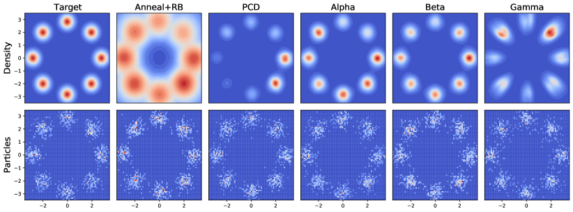
Figure 1: The top row depicts the learned densities for different approaches. Since method $\gamma$ doesn’t yield the parametric model for the energy, we integrate the energy numerically using $\partial E/\partial t$ from (15). The bottom row depicts the histograms of samples obtained in the end of learning procedures.

We empirically test the proposed methods $\alpha,\beta,\gamma$ and compare them against conventional approaches: PCD (Tieleman & Hinton, 2009) and sampling with Replay Buffer (Du & Mordatch, 2019). We found that for the stability of Replay Buffer it is important to reduce the noise magnitude (as also proposed in (Du & Mordatch, 2019)). That, however, yields sampling from an annealed target. For both “PCD” and “Anneal + RB”, we make $20$ steps of stochastic Langevin on every iteration. For our methods we propagate the particles along the corresponding vector fields and make additional $10$ steps of stochastic Langevin to alleviate possible numerical errors. For the target distribution we take toy 2-d distribution, and try to match it with 2-layer fully-connected neural network ($300$ hidden units, Swish activations (Ramachandran et al., 2017)). For method gamma, we found that using the same parameters $\theta$ throughout the learning leads to degenerate solutions. Therefore, we sample using the kernel $k_{\theta}(x,y)=\mathbb{E}_{\theta\sim\pi_{0}}\langle\nabla_{\theta}E(x,\theta),\nabla_{\theta}E(y,\theta)\rangle$, where parameters $\theta$ are sampled from the initialization distribution $\pi_{0}$ at each iteration, i.e. we use unlearned random networks to propagate particles.

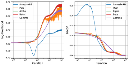
Figure 2: Performance of the models throughout the training. The quality of the energy as measured by the log-likelihood, and the MMD² between current set of particles and the training batch. Note that the Alpha’s plot is just under the Beta’s plot.

In Fig. 1, we demonstrate the learned densities and the particles. In Fig. 2, we report the metrics for models and samples averaging over $10$ independent runs. We don’t report standard errors to keep the plots readable. As we see, only $\alpha$ and $\beta$ nicely capture all of the modes. We found the learning via PCD to be the most unstable and unable to capture all of the modes in most cases. Annealing with the Replay Buffer is the most stable method in our experiments. However, it yields the density with scaled temperature due to the incorrect noise magnitude. Finally, we conclude that the proposed methods demonstrate better performance with a lower computational budget. Interestingly, all of the methods manage to match the final set of particles with the target distribution regardless of the learned energy.

6 Conclusion

We approach the problem of sampling from a distribution evolving in time, which is especially important in the context of energy-based learning. Our main contribution is the approximate formula for the vector field that propagates the particles matching the evolution of the distribution. We demonstrate that this formula yields several reasonable algorithms connected to deterministic Langevin and MMD gradient flows. Intuitively, method $\alpha$ moves the particles matching the new energy and, at the same time, unmatching the old energy. In contrast, methods $\beta$ and $\gamma$ propel particles aiming the target data distribution and repelling particles from each other to cover the state-space. Finally, we show that our deterministic approach can be favorable in practice for learning energy-based models.

Appendix A Proof of proposition 1

Proposition.

The solution of

$$v^{*}=\operatorname*{max\cdot arg\,max}_{v\in L^{2}_{q}:\left\lVert v\right\rVert=1}\bigg{\langle}\frac{\partial}{\partial t}\log q_{t},\frac{\partial}{\partial t}\log\hat{q}_{t}\bigg{\rangle}_{L_{q}^{2}}$$ (20)

is $v^{*}=-\nabla\frac{\partial E}{\partial t}$.

Proof.

The evolution of $\hat{q}_{t}$ is evolution defined by the vector field $v$, i.e.

$$\frac{\partial}{\partial t}\log\hat{q}_{t}=\frac{1}{\hat{q}_{t}}\frac{\partial\hat{q}_{t}}{\partial t}=-\langle\nabla\log q_{t},v\rangle-\langle\nabla,v\rangle,$$ (21)

and the first argument of the scalar product is defined by the updates of the energy

$$\frac{\partial}{\partial t}\log q_{t}=-\frac{\partial E}{\partial t}+\mathbb{E}_{q_{t}}\frac{\partial E}{\partial t}.$$ (22)

We rewrite the scalar product in (20) as

$$\bigg{\langle}\frac{\partial}{\partial t}\log q_{t},\frac{\partial}{\partial t}\log\hat{q}_{t}\bigg{\rangle}_{L_{q}^{2}} =\int dxq\bigg{[}\frac{\partial E}{\partial t}-\mathbb{E}_{q_{t}}\frac{\partial E}{\partial t}\bigg{]}\bigg{[}\langle\nabla\log q_{t},v\rangle+\langle\nabla,v\rangle\bigg{]}=$$ (23)

$$=\int dxq\frac{\partial E}{\partial t}\bigg{[}\langle\nabla\log q_{t},v\rangle+\langle\nabla,v\rangle\bigg{]}-\mathbb{E}_{q_{t}}\frac{\partial E}{\partial t}\int dxq\frac{1}{q}\frac{\partial q}{\partial t}=$$ (24)

$$=\int dxq\frac{\partial E}{\partial t}\bigg{[}\langle\nabla\log q_{t},v\rangle+\langle\nabla,v\rangle\bigg{]}.$$ (25)

Integrating by parts, we have

$$\bigg{\langle}\frac{\partial}{\partial t}\log q_{t},\frac{\partial}{\partial t}\log\hat{q}_{t}\bigg{\rangle}_{L_{q}^{2}} =\int dx\bigg{\langle}\frac{\partial E}{\partial t}\nabla q-\nabla\big{(}q\frac{\partial E}{\partial t}\big{)},v\bigg{\rangle}=$$ (26)

$$=\int dxq\bigg{\langle}-\nabla\frac{\partial E}{\partial t},v\bigg{\rangle}=\bigg{\langle}-\nabla\frac{\partial E}{\partial t},v\bigg{\rangle}_{L_{q}^{2}}.$$ (27)

∎

Appendix B Proof of proposition 2

Proposition.

Consider the functional $F=\int f(q)$, which we can optimize either w.r.t. $q=\exp(-E)/Z$ or w.r.t. $E$. Vector fields $v^{*}=v^{\star}$ when the evolution of the density (energy) is defined by the Frechet derivatve of $F$.

Proof.

The directional derivative (along the direction $h\in L^{2}$) is

$$\mathrm{diff}F(q)[h]=\bigg{\langle}\frac{\delta F(q)}{\delta q},h\bigg{\rangle}_{L^{2}},\;\;\;\frac{\delta F(q)}{\delta q}h=\frac{d}{d\varepsilon}f(q+\varepsilon h)\big{|}_{\varepsilon=0}.$$ (28)

We can think of $\frac{\delta F(q)}{\delta q}$ as of the formal symbolic application of differention rules. Then

$$v^{\star}=\nabla\frac{\partial q}{\partial t}=\nabla\frac{\delta F(q)}{\delta q},$$ (29)

which coincides with the vector field given by the Otto Calculus (Otto, 2001). For the energy, we consider the direction $h\in L^{2}_{q}$, then we have

$$\mathrm{diff}F(E)[h]=\int\frac{\delta F(q)}{\delta q}\frac{\delta q(E)}{\delta E}h=\bigg{\langle}-\frac{\delta F(q)}{\delta q}+\mathbb{E}_{q}\frac{\delta F(q)}{\delta q},h\bigg{\rangle}_{L^{2}_{q}}.$$ (30)

Finally, we see that the two derivatives yield the same vector-field.

$$v^{*}=-\nabla\frac{\partial E}{\partial t}=-\nabla\bigg{[}-\frac{\delta F(q)}{\delta q}+\mathbb{E}_{q}\frac{\delta F(q)}{\delta q}\bigg{]}=v^{\star}$$ (31)

∎

Appendix C Proof of proposition 3

Proposition.

The vector field $v^{*}=-\nabla\frac{\partial E}{\partial t}$ may be approximated by the “conventional update rule” of the particles following the Langevin dynamics targeting the updated density $q_{t+dt}$.

Proof.

Let’s approximate the vector field $v^{*}$ as

$$v^{*}\approx-\nabla\frac{1}{dt}\bigg{[}E_{t+dt}-E_{t}\bigg{]}=\frac{1}{dt}\bigg{[}\nabla\log q_{t+dt}-\nabla\log q_{t}\bigg{]},$$ (32)

Then the evolution of the density is described by the FP equation:

$$\dot{q}=-\langle\nabla,q_{t}v^{*}\rangle=-\langle\nabla,q_{t}\frac{1}{dt}\nabla\log q_{t+dt}\rangle+\frac{1}{dt}\Delta q_{t}.$$ (33)

Hence the evolution of particles can be described by the Ito equation

$$x_{t+dt^{\prime}}=x_{t}+dt^{\prime}\frac{1}{dt}\nabla\log q_{t+dt}(x_{t})+\sqrt{\frac{2}{dt}}dW_{t},$$ (34)

where $dW_{t}$ is the Wiener process, which can be simulated by the normal random variable $\mathcal{N}(0,dt^{\prime})$. Taking $dt^{\prime}=dt$, we have the conventional update rule (up to the step size choice)

$$x_{t+dt}=x_{t}+\nabla\log q_{t+dt}(x_{t})+\sqrt{2}\mathcal{N}(0,1)=x_{t}-\nabla E_{t+dt}(x_{t})+\sqrt{2}\mathcal{N}(0,1).$$ (35)

∎

Appendix D Proof of Proposition 4

Proposition.

The convergence of (16) is described by the equation:

$$\frac{d}{dt}{\mathrm{KL}}(p,q_{t})=-\mathrm{MMD}_{k}(p,q_{t})^{2}.$$ (36)

Proof.

$$\mathrm{diff}{\mathrm{KL}}(p,q)[h] =\langle p/q-1,h\rangle_{L^{2}_{q}}=\langle\underbrace{\mathbb{E}_{x\sim p}k(x,\cdot)-\mathbb{E}_{x\sim q}k(x,\cdot)}_{\partial E/\partial t},h\rangle_{\mathcal{H}}$$ (37)

$$\frac{d}{dt}{\mathrm{KL}}(p,q_{t})= -\mathbb{E}_{x\sim p}\frac{d}{dt}\log q_{t}(x)=\mathbb{E}_{x\sim p}\frac{\partial}{\partial t}E(x)-\mathbb{E}_{x\sim q_{t}}\frac{\partial}{\partial t}E(x)=$$ (38)

$$= \mathbb{E}_{x^{\prime}\sim p}\big{[}\mathbb{E}_{x\sim q_{t}}k(x,x^{\prime})-\mathbb{E}_{x\sim p}k(x,x^{\prime})\big{]}-$$ (39)

$$-\mathbb{E}_{x^{\prime}\sim q_{t}}\big{[}\mathbb{E}_{x\sim q_{t}}k(x,x^{\prime})-\mathbb{E}_{x\sim p}k(x,x^{\prime})\big{]}=$$ (40)

$$= -\mathbb{E}_{x,x^{\prime}\sim p}k(x,x^{\prime})+2\mathbb{E}_{x\sim p,x^{\prime}\sim q_{t}}k(x,x^{\prime})-\mathbb{E}_{x,x^{\prime}\sim q_{t}}k(x,x^{\prime})=$$ (41)

$$= -\mathrm{MMD}_{k}(p,q_{t})^{2}.$$ (42)

∎

References

- Arbel et al. (2019) Michael Arbel, Anna Korba, Adil Salim, and Arthur Gretton. Maximum mean discrepancy gradient flow. arXiv preprint arXiv:1906.04370, 2019.
- Arbel et al. (2020) Michael Arbel, Liang Zhou, and Arthur Gretton. Generalized energy based models. arXiv preprint arXiv:2003.05033, 2020.
- Benamou & Brenier (2000) Jean-David Benamou and Yann Brenier. A computational fluid mechanics solution to the monge-kantorovich mass transfer problem. Numerische Mathematik, 84(3):375–393, 2000.
- Du & Mordatch (2019) Yilun Du and Igor Mordatch. Implicit generation and generalization in energy-based models. arXiv preprint arXiv:1903.08689, 2019.
- Duncan et al. (2019) Andrew Duncan, Nikolas Nüsken, and Lukasz Szpruch. On the geometry of stein variational gradient descent. arXiv preprint arXiv:1912.00894, 2019.
- Gao et al. (2020) Ruiqi Gao, Yang Song, Ben Poole, Ying Nian Wu, and Diederik P Kingma. Learning energy-based models by diffusion recovery likelihood. arXiv preprint arXiv:2012.08125, 2020.
- Gelfand & Mitter (1991) Saul B Gelfand and Sanjoy K Mitter. Recursive stochastic algorithms for global optimization in r^d. SIAM Journal on Control and Optimization, 29(5):999–1018, 1991.
- Grathwohl et al. (2019) Will Grathwohl, Kuan-Chieh Wang, Jörn-Henrik Jacobsen, David Duvenaud, Mohammad Norouzi, and Kevin Swersky. Your classifier is secretly an energy based model and you should treat it like one. arXiv preprint arXiv:1912.03263, 2019.
- Grathwohl et al. (2020) Will Grathwohl, Kuan-Chieh Wang, Jörn-Henrik Jacobsen, David Duvenaud, and Richard Zemel. Learning the stein discrepancy for training and evaluating energy-based models without sampling. In International Conference on Machine Learning, pp. 3732–3747. PMLR, 2020.
- Gretton et al. (2012) Arthur Gretton, Karsten M Borgwardt, Malte J Rasch, Bernhard Schölkopf, and Alexander Smola. A kernel two-sample test. The Journal of Machine Learning Research, 13(1):723–773, 2012.
- Li et al. (2020) Shuang Li, Yilun Du, Gido M van de Ven, and Igor Mordatch. Energy-based models for continual learning. arXiv preprint arXiv:2011.12216, 2020.
- Liu et al. (2019) Chang Liu, Jingwei Zhuo, and Jun Zhu. Understanding mcmc dynamics as flows on the wasserstein space. In International Conference on Machine Learning, pp. 4093–4103. PMLR, 2019.
- Nijkamp et al. (2019) Erik Nijkamp, Mitch Hill, Song-Chun Zhu, and Ying Nian Wu. Learning non-convergent non-persistent short-run mcmc toward energy-based model. arXiv preprint arXiv:1904.09770, 2019.
- Otto (2001) Felix Otto. The geometry of dissipative evolution equations: the porous medium equation. 2001.
- Ramachandran et al. (2017) Prajit Ramachandran, Barret Zoph, and Quoc V Le. Searching for activation functions. arXiv preprint arXiv:1710.05941, 2017.
- Tieleman & Hinton (2009) Tijmen Tieleman and Geoffrey Hinton. Using fast weights to improve persistent contrastive divergence. In Proceedings of the 26th annual international conference on machine learning, pp. 1033–1040, 2009.