The Implicit Values of A Good Hand Shake:
Handheld Multi-Frame Neural Depth Refinement

Abstract

Modern smartphones can continuously stream multi-megapixel RGB images at 60 Hz, synchronized with high-quality 3D pose information and low-resolution LiDAR-driven depth estimates. During a snapshot photograph, the natural unsteadiness of the photographer’s hands offers millimeter-scale variation in camera pose, which we can capture along with RGB and depth in a circular buffer. In this work we explore how, from a bundle of these measurements acquired during viewfinding, we can combine dense micro-baseline parallax cues with kilopixel LiDAR depth to distill a high-fidelity depth map. We take a test-time optimization approach and train a coordinate MLP to output photometrically and geometrically consistent depth estimates at the continuous coordinates along the path traced by the photographer’s natural hand shake. With no additional hardware, artificial hand motion, or user interaction beyond the press of a button, our proposed method brings high-resolution depth estimates to point-and-shoot “tabletop” photography – textured objects at close range.

1 Introduction

The cell-phone of the 90s was a phone, the modern cell-phone is a handheld computational imaging platform [9] that is capable of acquiring high-quality images, pose, and depth. Recent years have witnessed explosive advances in passive depth imaging, from single-image methods that leverage large data priors to predict structure directly from image features [40, 41] to efficient multi-view approaches grounded in principles of 3D geometry and epipolar projection [50, 47]. At the same time, progress has been made in the miniaturization and cost-reduction [3] of active depth systems such as LiDAR and correlation time-of-flight sensors [29]. This has culminated in their leap from industrial and automotive applications [45, 11] to the space of mobile phones. Nestled in the intersection of high-resolution imaging and miniaturized LiDAR we find modern smartphones, such as the iPhone 12 Pro, which offer access to high frame-rate, low-resolution depth and high-quality pose estimates.

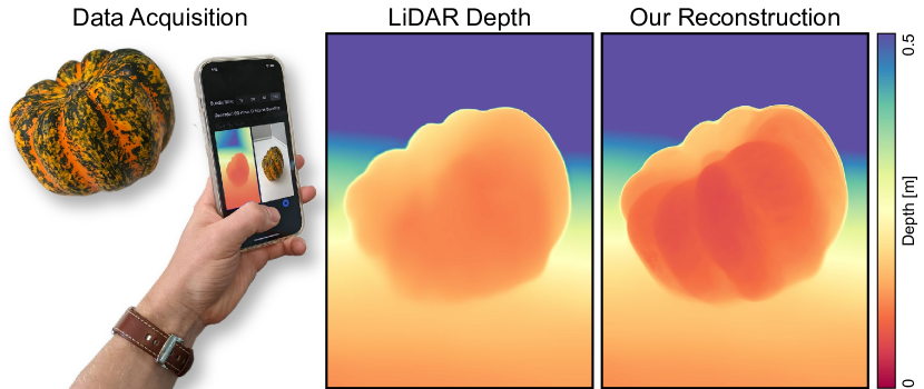
Figure 1: We reconstruct centimeter-scale depth features for this tabletop object from nothing more than a handheld snapshot.

As applications of mixed reality grow, particularly in industry [30] and healthcare [17] settings, so does the demand for convenient systems to extract 3D information from the world around us. Smartphones fit this niche well, as they boast a wide array of sensors – e.g. cameras, magnetometer, accelerometer, and the aforementioned LiDAR system – while remaining portable and affordable, and consequently ubiquitous. Image, pose, and depth data from mobile phones can drive novel problems in view synthesis [35, 39], portrait relighting [38, 49], and video interpolation [2] that either implicitly or explicitly rely on depth cues, as well as more typical 3D understanding tasks concerning salient object detection [59, 13], segmentation [46], localization [61], and mapping [44, 37].

Although 3D scene information is essential for a wide array of 3D vision applications, today’s mobile phones do not offer accurate high-resolution depth from a single snapshot. While RGB image data is available at more than 100 megapixels (e.g. Samsung ISOCELL HP1), the most successful depth sensors capture at least three orders of magnitude fewer measurements, with pulsed time-of-flight sensors [36] and modulated correlation time-of-flight imagers [28, 20, 27] offering kilopixel resolutions. Passive approaches can offer higher spatial resolution by exploiting RGB data; however, existing methods relying on stereo [7, 4, 25] depth estimation require large baselines, monocular depth methods [6, 40] suffer from scale ambiguity, and structure-from-motion methods [43] require diverse poses that are not present in a single snapshot. Accurate high-resolution snapshot depth remains an open challenge.

For imaging tasks, align and merge computational photography approaches have long exploited subtle motion cues during a single snapshot capture. These take advantage of the photographer’s natural hand tremor during viewfinding to capture a sequence of slightly misaligned images, which are fused into one super-resolved image [55, 51]. These misaligned frames can also be seen as mm-baseline stereo pairs, and works such as [57, 24] find that they contain enough parallax information to produce coarse depth estimates. Unfortunately, this micro-baseline depth is not enough to fuel mixed reality applications alone, as it lacks the ability to segment clear object borders or detect cm-scale depth features. In tandem with high-quality poses from phone-based SLAM [12] and low-resolution LiDAR depth maps, however, we can use the high-resolution micro-baseline depth cues to guide the reconstruction of a refined high-resolution depth map. We develop a pipeline for recording LiDAR depth, image, and pose bundles at 60 Hz, with which we can conveniently record 120 frame bundles of measurements during a single snapshot event.

With this hand shake data in hand, we take a test-time optimization approach to distill a high-fidelity depth estimate from hand tremor measurements. Specifically, we learn an implicit neural representation of the scene from a bundle of measurements. Depth represented by a coordinate multilayer perceptron (MLP) allows us to query for depth at floating point coordinates, which matches our measurement model, as we effectively traverse a continuous path of camera coordinates during the movement of the photographer’s hand. We can, during training, likewise conveniently incorporate parallax and LiDAR information as photometric and geometric loss terms, respectively. In this way we search for an accurate depth solution that is consistent with low-resolution LiDAR data, aggregates depth measurements across frames, and matches visual features between camera poses similar to a multi-view stereo approach. Specifically, we make the following contributions

• A smartphone app with a point-and-shoot user interface for easily capturing synchronized RGB, LiDAR depth, and pose bundles in the field.

• An implicit depth estimation approach that aggregates this data bundle into a single high-fidelity depth map.

• Quantitative and qualitative evaluations showing that our depth estimation method outperforms existing single and multi-frame techniques.

The smartphone app, training code, experimental data, and trained models are available at github.com/princeton-computational-imaging/HNDR .

2 Related Work

Active Depth Imaging.  Active depth methods prove a scene with a known illumination pattern and use the returned signal to reconstruct depth. Structured light approaches use this illumination to improve local image contrast [58, 42] and simplify the stereo-matching process. Time-of-Flight (ToF) technology instead uses the travel time of the light itself to measure distances. Indirect ToF achieves this through measuring the phase differences in the returned light [28], whereas direct ToF methods time the departure and return of pulses of light via avalanche photodiodes [8] or single-photon detectors (SPADs) [34]. The low spatial-resolution depth stream we use in this work relis on a LiDAR direct ToF sensor. While its mobile implementation comes with the caveats of low-cost SPADs [3] and vertical-cavity surface-emitting lasers [53], with limited spatial resolution and susceptibility to surface reflectance, this sensor can provide robust metric depth estimates, without scale ambiguity, on even visually textureless surfaces. We use this LiDAR depth data to regularize our network’s outputs, avoiding local minima solutions for low-texture regions.

Multi-View Stereo.  Multi-view stereo (MVS) algorithms are passive depth estimation methods that infer the 3D shape of a scene from a bundle of RGB views and, optionally, associated camera poses. COLMAP [43] estimates both poses and sparse depths by matching visual features across frames. The apparent motion of each feature in image space is uniquely determined by its depth and camera pose. Thus there exists an important relationship that, for a noiseless system, any pixel movement (disparity) not caused by a change in pose must be caused by a change in depth. While classical approaches typically formulate this as an explicit photometric cost optimization [48, 15, 16], more recent learning-based approaches bend the definition of cost with learned visual features [56, 50, 32], which aid in dense matching as they incorporate non-local information into otherwise textureless regions and are more robust to variations in lighting and noise that distort RGB values. In our setup, with little variation in lighting or appearance and free access to reliable LiDAR-based depth estimates in textureless regions, we look towards photometric MVS to extract parallax information from our images and poses.

Monocular Depth Prediction.  Single-image monocular approaches [41, 40, 18] offer visually reasonable depth maps, where foreground and background objects are clearly separated but may not be at a correct scale, with minimal data requirements – just a single image. Video-based methods such as [14, 33, 54] leverage structure-from-motion cues [52] to extract additional information on scene scale and geometry. Works such as [19, 23] use video data with small (decimeter-scale) motion, and [24, 57] explore micro-baseline (mm-scale) motion. As the baseline decreases, the depth estimation problem gradually devolves from MVS to effectively single-image prediction. Our work resides in the micro-baseline domain, using only millimeters of baseline information, but leverages metric LiDAR depth and pose information to bypass the noisy search for affine depth solutions – the cycle of identifying and matching sparse image features – that previous works were forced to contend with.

3 Neural Micro-baseline Depth

Overview.  When capturing a “snapshot photograph” on a modern smartphone, the simple interface hides a significant amount of complexity. The photographer typically composes a shot with the assistance of an electronic viewfinder, holding steady before pressing the shutter. During composition, a modern smartphone streams the recent past, consisting of synchronized RGB, depth, and six degree of freedom pose (6DoF) frames into a circular buffer at 60 Hz.

In this setting, we make the following observations: (1) A few seconds is sufficient for a typical snapshot of a static object. (2) During composition, the amount of hand shake is small (mm-scale). (3) Under small pose changes view-dependent lighting effects are minor. (4) Our data shows that current commercial devices have excellent pose estimation, likely due to well-calibrated sensors (IMU, LiDAR, RGB camera) collaborating to solve a smooth low-dimensional problem. Concretely, at each shutter press, we capture a “data bundle” of time-synchronized frames, each consisting of an RGB image $I$, 3D poses $P$, camera intrinsics $K$, and a depth map $Z$. In our experiments, the high-resolution RGB is 1920$\times$1440, while the LiDAR depth is 256 $\times$ 192. To save memory, we restrict bundles to $N=120$ frames (two seconds) in all our experiments.

Micro-Baseline parallax.  We specialize classical multi-view stereo [21] for our small motion scenario. Without loss of generality, we denote the first frame in our bundle the reference (r) and represent all other query (q) poses using the small angle approximation relative to the reference

$$P_{q}=\left[\begin{array}[]{c|c}R(\bm{r})&\bm{t}\end{array}\right]\approx\left[\begin{array}[]{ccc|c}1&-\bm{r}^{z}&\bm{r}^{y}&\bm{t}^{x}\\ \bm{r}^{z}&1&-\bm{r}^{x}&\bm{t}^{y}\\ -\bm{r}^{y}&\bm{r}^{x}&1&\bm{t}^{z}\\ \end{array}\right].$$ (1)

Let $X$ the homogeneous coordinates of a 3D point $(x,y,z,1)^{\top}$, the geometric consistency constraint is

$$X_{r}=P_{q}X_{q}.$$ (2)

In other words, the known pose should transform any 3D point in the query frame to its corresponding 3D location in the reference frame. Given camera intrinsics $K_{r},K_{q}$, with

$$K=\left[\begin{array}[]{ccc}f_{x}&0&c_{x}\\ 0&f_{y}&c_{y}\\ 0&0&1\end{array}\right],$$ (3)

and a point $X$ perspective projection yields continuous pixel coordinates $\bm{x}_{r},\bm{x}_{q}$ via

$$\bm{x}=\bm{\pi}(KX)=\left[\begin{array}[]{c}u=\nicefrac{{f_{x}x}}{{z}}+c_{x}\\ v=\nicefrac{{f_{y}y}}{{z}}+c_{y}\end{array}\right].$$ (4)

Using these pixel coordinates to sample from images $I_{r}$ and $I_{q}$, we arrive at our second constraint

$$I_{r}(\bm{x}_{r}=\bm{\pi}(K_{r}P_{q}X_{q}))=I_{q}(\bm{x}_{q}).$$ (5)

Corresponding 3D points should be photometrically consistent: with small motion, they should have the same color in both views. These two constraints are visualized in Fig. 2. To generate a 3D point $X(\bm{x},z)$ we can “unproject” a pixel coordinate $\bm{x}$ at depth $z=Z(\bm{x})$ by way of

$$X(\bm{x},z)=\bm{\pi}^{-1}(\bm{x},z;K)=\left[\begin{array}[]{c}z(u-c_{x})/f_{x}\\ z(v-c_{y})/f_{y}\\ z\\ 1\end{array}\right].$$ (6)

Our objective is to find a refined depth representation $Z^{\prime}$ such that for all $z\in Z^{\prime}$ any unprojected point $X(\bm{x})$ best satisfies our geometric (2) and photometric (5) constraints for all query views.

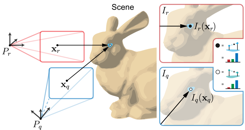
Figure 2: Visualization of how we project points $\bm{x}_{r},\bm{x}_{q}$ with corresponding camera poses $P_{r},P_{q}$ to 3D space and bilinearly sample image points $I_{r}(\bm{x}_{r})$ and $I_{q}(\bm{x}_{q})$. Note that the pose change here is enlarged for ease of illustration, the real misalignment in views from hand shake is on the scale of millimeters.

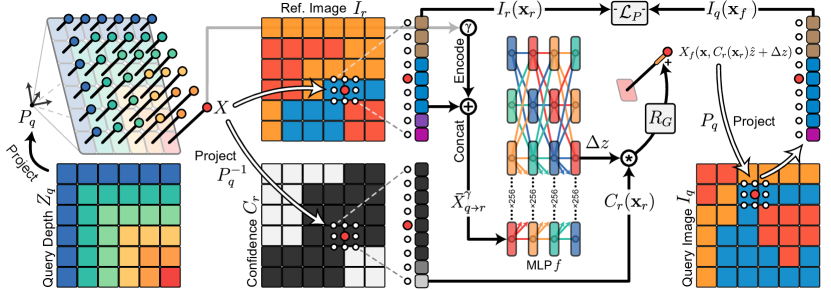
Figure 3: An illustrated pipeline of our proposed model. The query depth is used to project and sample a patch from our reference image $I_{r}$ for input into the MLP. This is weighed by a sample patch from our confidence $C_{r}$ to produce a depth offset $C_{r}(\bm{x_{r}})\Delta z$, which is used to project back to our query image $I_{q}$ and sample an image patch for loss calculation.

Implicit Depth Representation.  There are numerous ways with which we can represent $Z^{\prime}$. For example, we can represent it explicitly with a discrete depth map from the reference view, or as a large 3D point cloud. While explicit representations have many advantages (fast data retrieval, existing processing tools), they are also challenging to optimize. Depth maps are discrete arrays and merging multiple views at continuous coordinates requires resampling. This blurs fine-scale information and is non-trivial at occlusion boundaries. Point cloud representations trade off this adaptive filtering problem with one of scale. Not only is a two second sequence with 120 million points unwieldy for conventional tools [1], the points are almost entirely redundant.

Thus, we choose an implicit depth representation in the form of a coordinate multi-layer perceptron (MLP) [22], where its learnable parameters automatically adapt to the scene structure. Recent work have used MLPs to great success in neural rendering [35, 5, 39] and depth-estimation, where a continuous representation is of interest [60]. In our application, the MLP is a differentiable function

$$z^{\prime}=Z^{\prime}(\bm{x})=f(\mathrm{inputs};\theta)$$ (7)

returning a continuous $z^{\prime}$ given an encoding of position, camera pose, color, and other features. In our implementation, $\mathrm{inputs}$ is a positionally encoded 3D colored point

$$\bar{X}^{\gamma}=[\gamma(x),\gamma(y),\gamma(z),r,g,b]^{\top}.$$ (8)

We follow the encoding of [35] with

$$\gamma(p)=\left[\sin\left(2^{0}\pi p\right),\cos\left(2^{0}\pi p\right),\ldots,\cos\left(2^{L-1}\pi p\right)\right],$$ (9)

where $L$ is a selected number of encoding functions, and $r,g,b$ are color values scaled to $[0,1]$. As the size of this MLP is fixed, the large dimensionality of our measurements does not affect the calculation of $z^{\prime}$, and instead becomes a large training dataset from which to sample. Translating (2) and (5) into a regularized loss function on $z^{\prime}$, and backpropagating through $f$, our implicit depth representation $\theta$ can be learned with stochastic gradient descent.

Backward-Forward Projection Model.  Fig. 3 illustrates how we combine geometric and photometric constraints to optimize our MLP to produce a refined depth. At each training step we sample a query view $(I_{q},P_{q},Z_{q})$ and generate $M$ randomly sampled colored points $\bar{X}_{q}$ via Eq. 6

$$\bar{X}_{q}=\left[\begin{array}[]{c}\left[x,y,z,1\right]^{\top}\\ \left[r,g,b\right]^{\top}\end{array}\right]=\left[\begin{array}[]{c}X_{q}(\bm{x},z=Z_{q}(\bm{x}))\\ I_{q}(\bm{x})\end{array}\right]$$ (14)

$$\bm{x}=\left[u,v\right]^{\top},\quad u\sim\mathcal{U}(0,W),\quad v\sim\mathcal{U}(0,H),$$ (15)

where $H$ and $W$ are the image height and width, respectively. Here, $\bm{x}$ is a continuous coordinate and $I(\bm{x}),Z(\bm{x})$ represent sampling with a bilinear kernel. Following (2) we transform these points to the reference frame as

$$\bar{X}_{q\rightarrow r}=\left[\begin{array}[]{c}\left[\hat{x},\hat{y},\hat{z},1\right]^{\top}\\ I_{q}(\bm{x})\end{array}\right]=\left[\begin{array}[]{c}P_{q}X_{q}(\bm{x},z)\\ I_{q}(\bm{x})\end{array}\right].$$ (16)

Then, rather than directly predicting a refined depth $z^{\prime}$, we ask our MLP to predict a depth correction $\Delta z$, that is

$$\Delta z=f(\bar{X}^{\gamma}_{q\rightarrow r})$$ (17)

$$X_{f}(\bm{x},z^{\prime})=X_{f}(\bm{x},\hat{z}+\Delta z)=\left[\hat{x},\hat{y},\hat{z}+\Delta z,1\right]^{\top}.$$

As we show in Section 5, this parameterization allows us to avoid local minima in poorly textured regions. We transform these refined points $X_{f}$ back to the query frame and resample the query image at the updated coordinates

$$I_{q}(\bm{x}_{f})=I_{q}(\bm{\pi}(P_{q}^{-1}X_{f}(\bm{x},\hat{z}+\Delta z))).$$ (18)

Finally, our photometric loss is

$$\mathcal{L}_{P}=|I_{q}(\bm{x}_{f})-I_{r}(\bm{x}_{r})|^{2}$$

$$\bm{x}_{r}=\bm{\pi}(K_{r}P_{q}X_{q}(\bm{x},z)),$$ (19)

which attempts to satisfy (5) by encouraging the colors of the refined 3D points to be the same in both the query and reference frames. While (5) works well in well-textured areas, it is fundamentally underconstrained in flat regions. Therefore, we augment our loss with a weighted geometric regularization term based on (2) that pushes the solution towards an interpolation of LiDAR depth in these regions

$$\mathcal{R}_{G}=|X_{f}(\bm{x},\hat{z}+\Delta z)-P_{q}X_{q}(\bm{x},z))|\approx|\Delta z|.$$ (20)

Our final loss is a weighted combination of these two terms

$$\mathcal{L}=\mathcal{L}_{P}+\alpha\mathcal{R}_{G},$$ (21)

where by tuning $\alpha$ we adjust how strongly our reconstruction adheres to the LiDAR depth initialization.

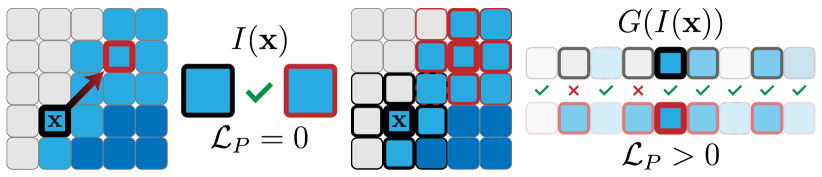
Figure 4: A weighted sampling around a point $\bm{x}$ we can avoid false matches in otherwise color-ambiguous image regions. Opacity and border thickness represents the weight of each sample.

Patch Sampling.  In practice, we cannot rely on single-pixel samples as written in (6) for photometric optimization. Our two megapixel input images $I$ will almost certainly contain color patches that are larger than the depth-induced motion of pixels within them. With single-pixel samples, there are many incorrect depth solutions that yield $\mathcal{L}_{P}$ of zero. To combat this, we replace each sample $I(\bm{x})$ in (14) with Gaussian-weighted patches

$$G(I(\bm{x}))=\left[\mathcal{N}(\sqrt{\delta_{u}^{2}+\delta_{v}^{2}};\mu,\sigma^{2})I(\bm{x}-[\delta_{u},\delta_{v}]^{\top})\right],$$

$$\mathrm{for}\quad\delta_{u}=\left\{-K\ldots K\right\},\;\delta_{v}=\left\{-K\ldots K\right\}.$$ (22)

Fig. 4 illustrates this for $K=3$: the increased receptive field discourages false color matches. Adjusting $K$, we trade off the ability to reconstruct fine features for robustness to noise and low-contrast textures (see supplement).

Explicit Confidence.  Another augmentation we make is to introduce a learned explicit $H\times W$ confidence map $C_{r}$ to weigh the MLP outputs. That is, we replace $\Delta z$ with $C_{r}(\bm{x}_{r})\Delta z$ in (17). This additional degree of freedom allows the network push $\Delta z$ toward zero in color-ambiguous regions, rather than forcing it to first learn a positional mapping of where these regions are located in the image. As $C_{r}(\bm{x}_{r})$ only adds an additional sampling step during point generation, the overhead is minimal. Once per epoch we apply an optional $5\times 5$ median filter to $C_{r}$ to minimize the effects of sampling noise during training.

Final reconstruction.  After training, to recover a refined depth map $Z^{*}$ we begin by reprojecting all low-resolution depth maps $Z_{q}$ to the reference frame following (2). We then average and bilinearly resample this data to produce a $H\times W$ depth map $Z_{avg}$. We query the MLP at $H\times W$ grid-spaced points, using $I_{r}$ and $Z_{avg}$ to generate points as in (14). Finally, we extract and re-grid the depth channel from the MLP outputs $R_{f}$ to produce $Z^{*}$.

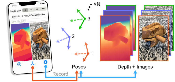
Figure 5: Our smartphone app for capturing data bundles, with two illustrated recording functions. The button to record only pose allows the user to save and analyze hundreds of hand motion bundles without the overhead of transferring tens of gigabytes of video.

4 Data Collection

Recording a Bundle.  We built a smartphone application for recording bundles of synchronized image, pose, and depth maps. Our app, running on an iPhone 12 Pro using ARKit 5, provides a real-time viewfinder with previews of RGB and depth (Fig. 5). The user can select bundle sizes of [15, 30, 60, 120] frames ([0.25, 0.5, 1, 2] seconds of recording time) and we save all data, including nanosecond-precision timestamps to disk. We will publish the code for both the app and our offline processing pipeline (which does color-space conversion, coordinate space transforms, etc.).

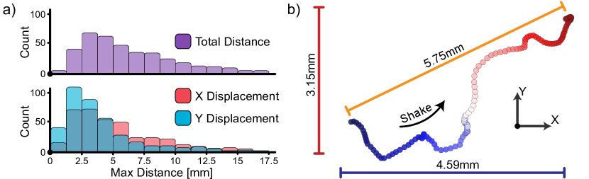
Figure 6: (a) Distribution of displacements in camera position during the capture of a 120 frame bundle in portrait mode. (b) Visualization of a hand tremor path with labeled median displacements.

Natural Hand Tremor Analysis.  To analyze hand motion during composition, we collected fifty 2-second pose-only bundles from 10 volunteers. Each was instructed to act as if they were capturing photos of objects around them, to hold the phone naturally in their dominant hand, and to keep focus on an object in the viewfinder. We illustrate our aggregate findings in Fig. 6 and individual measurements in the supplemental material. We focus on in-plane displacement they are the dominant contribution to observed parallax. We find that natural hand tremor appears similar to paths traced by 2D Brownian motion, with some paths traveling far from the initial camera position as in Fig. 6 (b), and others forming circles around the initial position. Consequently, while the median effective baseline from a two second sequence is just under 6mm, some recordings exhibit nearly 1cm of displacement, while others appear are almost static. We suspect that the effects of breathing and involuntary muscle twitches are greatly responsible for this variance. Herein lies the definition of good hand shake: it is one that produces a useful micro-baseline.

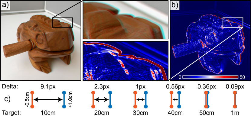
Figure 7: (a) Anaglyph visualization of maximum observed disparity for a 1m plane-rectified 120 frame image sequence. (b) Absolute difference between the frames in (a). (c) Observed disparity (Delta) with a 6mm baseline for a 1cm feature at depth (Target).

Fig. 7 (c) illustrates, given our smartphone’s optics, what a 6mm baseline translates to in pixel disparity and therefore the depth feature precision. We intentionally limit ourselves to a depth range of approximately 50 cm, beyond which image noise and errors in pose estimation overpower our ability to estimate subpixel displacement.

5 Assessment

Implementation Details.  We use $N=120$ frame bundles for our main experiments. Images are recorded in portrait orientation, with $H=1920$, $W=1440$. Our MLP is a 4 layer fully connected network with ReLU activations and a hidden layer size of 256. For training we use inputs of $M=4096$ colored points, a kernel size of $K=11$, and $L=6$ encoding functions. We use the Adam optimizer [26] with an initial learning rate of $10^{-5}$, exponentially decreased over $200$ epochs with a decay rate of $0.985$. We apply the geometric regularization $\mathcal{R}_{G}$ with weight $\alpha=0.01$. We provide ablation experiments on the effects of many of these parameters in the supplement. Training takes about 45 minutes on an NVIDIA Tesla P100 GPU, or 180 minutes on an Intel Xeon Gold 6148 CPU.

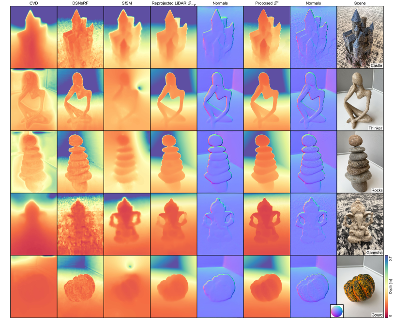
Figure 8: Qualitative comparison of depth reconstruction methods for tabletop scenes. Normals are shown for $Z_{avg}$ and our proposed method to highlight how we recover centimeter-scale features absent from the input depths. See the supplement for additional results.

Comparisons.  We compare our method (Proposed) to the input LiDAR data and several recent baselines. Namely, we reproject all the depth maps in our bundle to the reference frame and resample them to produce a $1920\times 1440$ LiDAR baseline $Z_{avg}$. For the depth reconstruction methods we look to Consistent Video Depth Estimation [33] (CVD), which similarly uses photometric loss between frames in a video to refine a consistent depth; Depth Supervised NeRF [10] (DSNeRF), which also features an MLP for depth prediction; and Structure from Small Motion [19] (SfSM), which investigates a closed-form solution to depth estimation from micro-baseline stereo. Both DSNeRF and CVD rely on COLMAP [43] for poses or depth inputs. However, when input our micro-baseline data, COLMAP fails to converge and returns neither. For fair comparison, we substitute our high-accuracy LiDAR poses and depths.

Scene	CVD [33]	DSNeRF [10]	SfSM [19]	$Z_{avg}$	Proposed
castle	4.88$/$62.9	4.89$/$87.3	4.70$/$55.4	4.51$/$48.1	3.83$/$30.0
thinker	4.73$/$115	4.59$/$109	5.78$/$170	4.50$/$107	4.26$/$89.4
rocks	6.68$/$212	5.83$/$180	6.43$/$190	5.52$/$163	4.59$/$97.3
ganesha	4.93$/$56.5	5.29$/$103	4.45$/$41.3	4.41$/$36.8	3.51$/$23.4
gourd	4.25$/$92.6	4.00$/$108	3.72$/$70.7	3.77$/$92.8	3.14$/$52.9
eagle	3.93$/$63.1	4.09$/$93.4	6.60$/$219	3.98$/$93.2	3.32$/$49.0
double	4.77$/$68.6	4.87$/$91.3	4.30$/$39.1	4.00$/$31.6	3.57$/$22.1
elephant	5.12$/$101	5.20$/$124	5.49$/$120	5.09$/$127	4.46$/$78.8
embrace	4.92$/$54.5	5.13$/$88.7	3.81$/$26.0	3.27$/$23.1	2.85$/$15.5
frog	3.44$/$68.2	3.11$/$58.9	3.05$/$51.5	2.80$/$49.9	2.58$/$34.1

Table 1: Quantitative comparison of photometric error for our ten tested scenes. Each entry shows: mean absolute error $/$ mean squared error. Note that different scenes can have different scales of error, as it is dependent on their overall image texture content.

Experimental Results.  We present our results visually in Fig. 8 and quantitatively in Table 1 in the form of photometric error (PE). To compute PE, we take the final depth map $Z^{*}$ output by each method, use the phone’s poses and intrinsics to project each color point in $I_{r}$ to all other frames, and compare their sampled RGB values:

$$PE=\Sigma|I_{q}(\bm{x}_{q})-I_{r}(\bm{x})|,\quad\bm{x}_{q}=\bm{\pi}(P_{q}^{-1}X^{*})$$

$$X^{*}=\bm{\pi}^{-1}(\bm{x},Z^{*}(\bm{x});K),\quad\bm{x}=[u,v]^{\top}.$$ (23)

We exclude points $\bm{x}$ that transform outside the image bounds. Similar to traditional camera calibration or stereo methods, in the absence of ground truth depth, PE serves as a measure of how consistent our estimated depth is with the observed RGB parallax.

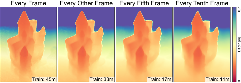
Figure 9: Frame count ablation with corresponding network train times. Note that due to various overheads, training time is not linear in the number of frames.

Table 1 summarizes the relative performance between these methods on 10 geometrically diverse scenes. Our method achieves the lowest PE for all scenes. Note that neither CVD nor DSNeRF achieve significantly lower PE as compared to the LiDAR depth $Z_{avg}$ even though both contain explicit photometric loss terms in their objective. We speculate that our micro-baseline data is out of distribution for these methods, and that the large loss gradients induced by small changes in pose results in unstable reconstructions. DSNeRF also has the added complexity of being a novel view synthesis method and is therefore encouraged to overfit to the scene RGB content in the presence of only small motion. We see this confirmed in Fig. 8, as DSNeRF produces an edge-aligned depth map but incorrect surface texture. SFsM successfully reconstructs textured regions close to the camera ($<$20cm), but fails for smaller disparity regions, textureless spaces, and parts of the image suffering from lens blur. The reprojected LiDAR depth produces well edge-aligned results but lacks intra-object structure, as it is relying on ambiguous mono-depth cues. Contrastingly, our proposed method reconstructs the castle’s towers, the hand under the thinker’s head, the depth disparity between stones in rocks, the trunk and arms of ganesha, and the smooth undulations of gourd. For visually complex scenes such as ganesha our method is able to cleanly separate the foreground object from its background.

Frame Ablation.  Though the average max baseline in a recorded bundle is  6mm, the baseline between neighboring frames is on the order of 0.1mm. This means that we need not use every frame for effective photometric refinement. This tradeoff between frame count, training time, and reconstruction detail is illustrated in Fig. 9. We retain most of the castle detail by skipping every other frame, and as we discard more data we see the reconstruction gradually lose fine edges and intra-object features.

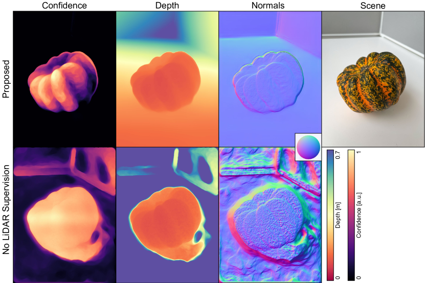
Figure 10: We reconstruct gourd without LiDAR supervision to better understand the effects of geometric regularization.

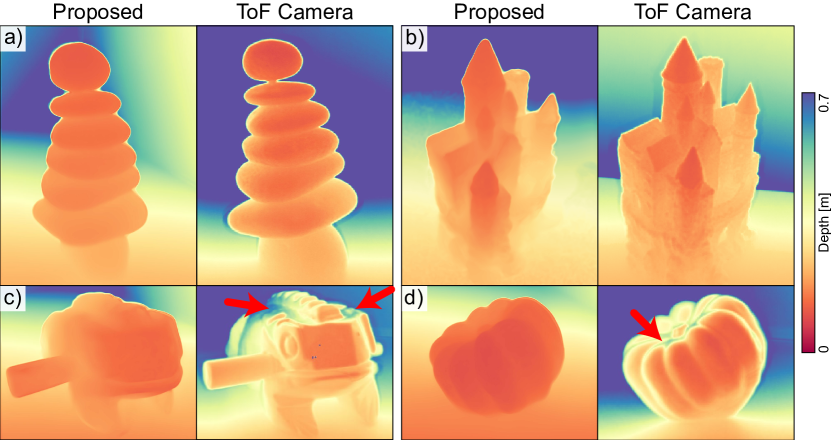
Figure 11: Qualitative comparison of proposed reconstruction results with depths captured by a time-of-flight camera. Examples (c) and (d) include arrows to highlight where the ToF camera suffers from severe multi-path interference artifacts and produces sharp depth discontinuities in place of expected smooth geometry.

Role of LiDAR Supervision.  To determine the contribution of the low-resolution LiDAR data in our pipeline, we perform an ablation where we set $Z\;{=}\;$1m and disable our geometric regularizer by setting $\alpha\;{=}\;0$. Fig. 10 shows that, as expected, it fails to reconstruct the textureless background. It does, however, correctly reconstruct the gourd, and produces a result similar to the pipeline with full supervision. This demonstrates that our method extracts most of its depth details from the micro-baseline RGB images. LiDAR depth, however, is an effective regularizer: in regions without strong visual features, our learned confidence map $C_{r}$ is nearly zero and our reconstruction gracefully degrades to the LiDAR data. Finally, we note that even though this ablation discards depth supervision, the LiDAR sensor is still used by the phone to produce high-accuracy poses.

Comparison to Dedicated ToF Camera.  We record several scenes with a high-resolution time-of-flight depth camera (LucidVision Helios Flex). Given the differences in optics and effective operating range, the viewpoints and metric depths do not perfectly match. We offset and crop (but don’t rescale) the depth maps for qualitative comparison. Fig. 11 validates that our technique can reconstruct centimeter-scale features matching that of the ToF sensor, but smooths finer details corresponding to subpixel disparities. Since we rely on passive RGB rather than direct illumination, our technique can reconstruct regions the ToF camera cannot such as specular surfaces on the back of frog and the top of gourd. In these cases, multi-path interference leads to incorrect amplitude modulated ToF measurements.

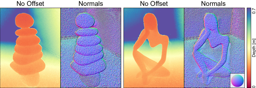
Figure 12: When we learn depth directly without a reasonable initialization we find that many samples end up stuck in local minima. This leads to noisy predictions where the MLP finds a false photometric matches far from the LiDAR depth estimate.

Offsets over Direct Depth.  Rather than directly learn $Z^{*}$, we opt to learn offsets to the collected LiDAR depth data. We effectively start at a coarse, albeit smooth, depth estimate and for each location in space, and search the local neighborhood for a more photometrically consistent depth solution. This allows us to avoid local minima solutions that overpower the regularization $\alpha R_{G}$ – e.g. accidentally matching similar image patches. This proves essential for objects with repetitive textures, as demonstrated in Fig. 12. Additional experiments can be found in the supplement.

6 Discussion and Future Work

We show that with a modern smartphone, its possible to reconstruct a high-fidelity depth map from just a snapshot of a textured “tabletop” object. We quantitatively validate that our technique outperforms several recent baselines and qualitatively compare to a dedicated depth camera.
Rolling Shutter. There is a delay in the tens of milliseconds between when we record the first and last row of pixels from the camera sensor [31], during which time the position of the phone could slightly shift. Given accurate shutter timings, one may incorporate a model of rolling shutter similar to [23] directly into the implicit depth model.
Training Time. Although our training time is practical for offline processing and opens the potential for the easy collection of a large-scale training corpus, our method may be further accelerated with an adaptive sampling scheme which takes into account pose, color, and depth information to select the most useful samples for network training.
Additional Sensors. We hope in the future to get access to raw phone LiDAR samples, whose photon time tags could provide an additional sparse high-trust supervision signal. Modern phones now also come with multiple cameras with different focal properties. If synchronously acquired, their video streams could expand the overall effective baseline of our setup and provide additional geometric information for depth reconstruction – towards snapshot smartphone depth imaging that exploits all available sensor modalities.
Acknowledgments.  Ilya Chugunov was supported by an NSF Graduate Research Fellowship. Felix Heide was supported by an NSF CAREER Award (2047359), a Sony Young Faculty Award, and a Project X Innovation Award.

References

- [1] K Somani Arun, Thomas S Huang, and Steven D Blostein. Least-squares fitting of two 3-d point sets. IEEE Transactions on pattern analysis and machine intelligence, (5):698–700, 1987.
- [2] Wenbo Bao, Wei-Sheng Lai, Chao Ma, Xiaoyun Zhang, Zhiyong Gao, and Ming-Hsuan Yang. Depth-aware video frame interpolation. In Proceedings of the IEEE/CVF Conference on Computer Vision and Pattern Recognition, pages 3703–3712, 2019.
- [3] Clara Callenberg, Zheng Shi, Felix Heide, and Matthias B Hullin. Low-cost spad sensing for non-line-of-sight tracking, material classification and depth imaging. ACM Transactions on Graphics (TOG), 40(4):1–12, 2021.
- [4] Jia-Ren Chang and Yong-Sheng Chen. Pyramid stereo matching network. In IEEE Conf. Comput. Vis. Pattern Recog., pages 5410–5418, 2018.
- [5] Anpei Chen, Zexiang Xu, Fuqiang Zhao, Xiaoshuai Zhang, Fanbo Xiang, Jingyi Yu, and Hao Su. Mvsnerf: Fast generalizable radiance field reconstruction from multi-view stereo. arXiv preprint arXiv:2103.15595, 2021.
- [6] Xiaozhi Chen, Kaustav Kundu, Ziyu Zhang, Huimin Ma, Sanja Fidler, and Raquel Urtasun. Monocular 3d object detection for autonomous driving. In IEEE Conf. Comput. Vis. Pattern Recog., pages 2147–2156, 2016.
- [7] Xiaozhi Chen, Kaustav Kundu, Yukun Zhu, Huimin Ma, Sanja Fidler, and Raquel Urtasun. 3d object proposals using stereo imagery for accurate object class detection. 40(5):1259–1272, 2017.
- [8] Sergio Cova, Massimo Ghioni, Andrea Lacaita, Carlo Samori, and Franco Zappa. Avalanche photodiodes and quenching circuits for single-photon detection. Applied optics, 35(12):1956–1976, 1996.
- [9] Mauricio Delbracio, Damien Kelly, Michael S Brown, and Peyman Milanfar. Mobile computational photography: A tour. arXiv preprint arXiv:2102.09000, 2021.
- [10] Kangle Deng, Andrew Liu, Jun-Yan Zhu, and Deva Ramanan. Depth-supervised nerf: Fewer views and faster training for free. arXiv preprint arXiv:2107.02791, 2021.
- [11] Pinliang Dong and Qi Chen. LiDAR remote sensing and applications. CRC Press, 2017.
- [12] Hugh Durrant-Whyte and Tim Bailey. Simultaneous localization and mapping: part i. IEEE robotics & automation magazine, 13(2):99–110, 2006.
- [13] Deng-Ping Fan, Zheng Lin, Zhao Zhang, Menglong Zhu, and Ming-Ming Cheng. Rethinking rgb-d salient object detection: Models, data sets, and large-scale benchmarks. IEEE Transactions on neural networks and learning systems, 32(5):2075–2089, 2020.
- [14] Michaël Fonder, Damien Ernst, and Marc Van Droogenbroeck. M4depth: A motion-based approach for monocular depth estimation on video sequences. arXiv preprint arXiv:2105.09847, 2021.
- [15] Yasutaka Furukawa and Jean Ponce. Accurate, dense, and robust multiview stereopsis. IEEE transactions on pattern analysis and machine intelligence, 32(8):1362–1376, 2009.
- [16] Silvano Galliani, Katrin Lasinger, and Konrad Schindler. Massively parallel multiview stereopsis by surface normal diffusion. In Proceedings of the IEEE International Conference on Computer Vision, pages 873–881, 2015.
- [17] Jaris Gerup, Camilla B Soerensen, and Peter Dieckmann. Augmented reality and mixed reality for healthcare education beyond surgery: an integrative review. International journal of medical education, 11:1, 2020.
- [18] Clément Godard, Oisin Mac Aodha, Michael Firman, and Gabriel J Brostow. Digging into self-supervised monocular depth estimation. In Proceedings of the IEEE/CVF International Conference on Computer Vision, pages 3828–3838, 2019.
- [19] Hyowon Ha, Sunghoon Im, Jaesik Park, Hae-Gon Jeon, and In So Kweon. High-quality depth from uncalibrated small motion clip. In Proceedings of the IEEE conference on computer vision and pattern Recognition, pages 5413–5421, 2016.
- [20] Miles Hansard, Seungkyu Lee, Ouk Choi, and Radu Patrice Horaud. Time-of-flight cameras: principles, methods and applications. Springer Science & Business Media, 2012.
- [21] Richard Hartley and Andrew Zisserman. Multiple View Geometry in Computer Vision. Cambridge University Press, USA, 2 edition, 2003.
- [22] Kurt Hornik, Maxwell Stinchcombe, and Halbert White. Multilayer feedforward networks are universal approximators. Neural networks, 2(5):359–366, 1989.
- [23] Sunghoon Im, Hyowon Ha, Gyeongmin Choe, Hae-Gon Jeon, Kyungdon Joo, and In So Kweon. Accurate 3d reconstruction from small motion clip for rolling shutter cameras. IEEE transactions on pattern analysis and machine intelligence, 41(4):775–787, 2018.
- [24] Neel Joshi and C Lawrence Zitnick. Micro-baseline stereo. Technical Report MSR-TR-2014–73, page 8, 2014.
- [25] Alex Kendall, Hayk Martirosyan, Saumitro Dasgupta, Peter Henry, Ryan Kennedy, Abraham Bachrach, and Adam Bry. End-to-end learning of geometry and context for deep stereo regression. In Int. Conf. Comput. Vis., 2017.
- [26] Diederik P Kingma and Jimmy Ba. Adam: A method for stochastic optimization. arXiv preprint arXiv:1412.6980, 2014.
- [27] Andreas Kolb, Erhardt Barth, Reinhard Koch, and Rasmus Larsen. Time-of-flight cameras in computer graphics. In Computer Graphics Forum, volume 29, pages 141–159. Wiley Online Library, 2010.
- [28] Robert Lange. 3d time-of-flight distance measurement with custom solid-state image sensors in cmos/ccd-technology. 2000.
- [29] Robert Lange and Peter Seitz. Solid-state time-of-flight range camera. IEEE Journal of quantum electronics, 37(3):390–397, 2001.
- [30] Xiao Li, Wen Yi, Hung-Lin Chi, Xiangyu Wang, and Albert PC Chan. A critical review of virtual and augmented reality (vr/ar) applications in construction safety. Automation in Construction, 86:150–162, 2018.
- [31] Chia-Kai Liang, Li-Wen Chang, and Homer H Chen. Analysis and compensation of rolling shutter effect. IEEE Transactions on Image Processing, 17(8):1323–1330, 2008.
- [32] Lahav Lipson, Zachary Teed, and Jia Deng. Raft-stereo: Multilevel recurrent field transforms for stereo matching. arXiv preprint arXiv:2109.07547, 2021.
- [33] Xuan Luo, Jia-Bin Huang, Richard Szeliski, Kevin Matzen, and Johannes Kopf. Consistent video depth estimation. ACM Transactions on Graphics (TOG), 39(4):71–1, 2020.
- [34] Aongus McCarthy, Robert J Collins, Nils J Krichel, Verónica Fernández, Andrew M Wallace, and Gerald S Buller. Long-range time-of-flight scanning sensor based on high-speed time-correlated single-photon counting. Applied optics, 48(32):6241–6251, 2009.
- [35] Ben Mildenhall, Pratul P Srinivasan, Matthew Tancik, Jonathan T Barron, Ravi Ramamoorthi, and Ren Ng. Nerf: Representing scenes as neural radiance fields for view synthesis. In European conference on computer vision, pages 405–421. Springer, 2020.
- [36] Kazuhiro Morimoto, Andrei Ardelean, Ming-Lo Wu, Arin Can Ulku, Ivan Michel Antolovic, Claudio Bruschini, and Edoardo Charbon. Megapixel time-gated spad image sensor for 2d and 3d imaging applications. Optica, 7(4):346–354, 2020.
- [37] Raul Mur-Artal and Juan D Tardós. Orb-slam2: An open-source slam system for monocular, stereo, and rgb-d cameras. IEEE transactions on robotics, 33(5):1255–1262, 2017.
- [38] Rohit Pandey, Sergio Orts Escolano, Chloe Legendre, Christian Haene, Sofien Bouaziz, Christoph Rhemann, Paul Debevec, and Sean Fanello. Total relighting: learning to relight portraits for background replacement. ACM Transactions on Graphics (TOG), 40(4):1–21, 2021.
- [39] Keunhong Park, Utkarsh Sinha, Jonathan T Barron, Sofien Bouaziz, Dan B Goldman, Steven M Seitz, and Ricardo Martin-Brualla. Nerfies: Deformable neural radiance fields. In Proceedings of the IEEE/CVF International Conference on Computer Vision, pages 5865–5874, 2021.
- [40] René Ranftl, Alexey Bochkovskiy, and Vladlen Koltun. Vision transformers for dense prediction. In Proceedings of the IEEE/CVF International Conference on Computer Vision, pages 12179–12188, 2021.
- [41] René Ranftl, Katrin Lasinger, David Hafner, Konrad Schindler, and Vladlen Koltun. Towards robust monocular depth estimation: Mixing datasets for zero-shot cross-dataset transfer. arXiv preprint arXiv:1907.01341, 2019.
- [42] Daniel Scharstein and Richard Szeliski. High-accuracy stereo depth maps using structured light. In 2003 IEEE Computer Society Conference on Computer Vision and Pattern Recognition, 2003. Proceedings., volume 1, pages I–I. IEEE, 2003.
- [43] Johannes L Schonberger and Jan-Michael Frahm. Structure-from-motion revisited. In Proceedings of the IEEE conference on computer vision and pattern recognition, pages 4104–4113, 2016.
- [44] Thomas Schops, Torsten Sattler, and Marc Pollefeys. Bad slam: Bundle adjusted direct rgb-d slam. In Proceedings of the IEEE/CVF Conference on Computer Vision and Pattern Recognition, pages 134–144, 2019.
- [45] Brent Schwarz. Mapping the world in 3d. Nature Photonics, 4(7):429–430, 2010.
- [46] Max Schwarz, Anton Milan, Arul Selvam Periyasamy, and Sven Behnke. Rgb-d object detection and semantic segmentation for autonomous manipulation in clutter. The International Journal of Robotics Research, 37(4-5):437–451, 2018.
- [47] Faranak Shamsafar, Samuel Woerz, Rafia Rahim, and Andreas Zell. Mobilestereonet: Towards lightweight deep networks for stereo matching. arXiv preprint arXiv:2108.09770, 2021.
- [48] Sudipta N Sinha, Philippos Mordohai, and Marc Pollefeys. Multi-view stereo via graph cuts on the dual of an adaptive tetrahedral mesh. In 2007 IEEE 11th International Conference on Computer Vision, pages 1–8. IEEE, 2007.
- [49] Tiancheng Sun, Jonathan T Barron, Yun-Ta Tsai, Zexiang Xu, Xueming Yu, Graham Fyffe, Christoph Rhemann, Jay Busch, Paul E Debevec, and Ravi Ramamoorthi. Single image portrait relighting. ACM Trans. Graph., 38(4):79–1, 2019.
- [50] Vladimir Tankovich, Christian Hane, Yinda Zhang, Adarsh Kowdle, Sean Fanello, and Sofien Bouaziz. Hitnet: Hierarchical iterative tile refinement network for real-time stereo matching. In Proceedings of the IEEE/CVF Conference on Computer Vision and Pattern Recognition, pages 14362–14372, 2021.
- [51] R Tsai. Multiframe image restoration and registration. Advance Computer Visual and Image Processing, 1:317–339, 1984.
- [52] Shimon Ullman. The interpretation of structure from motion. Proceedings of the Royal Society of London. Series B. Biological Sciences, 203(1153):405–426, 1979.
- [53] Mial E Warren, David Podva, Preethi Dacha, Matthew K Block, Christopher J Helms, John Maynard, and Richard F Carson. Low-divergence high-power vcsel arrays for lidar application. In Vertical-Cavity Surface-Emitting Lasers XXII, volume 10552, page 105520E. International Society for Optics and Photonics, 2018.
- [54] Jamie Watson, Oisin Mac Aodha, Victor Prisacariu, Gabriel Brostow, and Michael Firman. The temporal opportunist: Self-supervised multi-frame monocular depth. In Proceedings of the IEEE/CVF Conference on Computer Vision and Pattern Recognition, pages 1164–1174, 2021.
- [55] Bartlomiej Wronski, Ignacio Garcia-Dorado, Manfred Ernst, Damien Kelly, Michael Krainin, Chia-Kai Liang, Marc Levoy, and Peyman Milanfar. Handheld multi-frame super-resolution. ACM Transactions on Graphics (TOG), 38(4):1–18, 2019.
- [56] Yao Yao, Zixin Luo, Shiwei Li, Tian Fang, and Long Quan. Mvsnet: Depth inference for unstructured multi-view stereo. In Proceedings of the European Conference on Computer Vision (ECCV), pages 767–783, 2018.
- [57] Fisher Yu and David Gallup. 3d reconstruction from accidental motion. In Proceedings of the IEEE Conference on Computer Vision and Pattern Recognition, pages 3986–3993, 2014.
- [58] Song Zhang. High-speed 3d shape measurement with structured light methods: A review. Optics and Lasers in Engineering, 106:119–131, 2018.
- [59] Wenbo Zhang, Yao Jiang, Keren Fu, and Qijun Zhao. Bts-net: Bi-directional transfer-and-selection network for rgb-d salient object detection. In 2021 IEEE International Conference on Multimedia and Expo (ICME), pages 1–6. IEEE, 2021.
- [60] Zhoutong Zhang, Forrester Cole, Richard Tucker, William T Freeman, and Tali Dekel. Consistent depth of moving objects in video. ACM Transactions on Graphics (TOG), 40(4):1–12, 2021.
- [61] Chungang Zhuang, Zhe Wang, Heng Zhao, and Han Ding. Semantic part segmentation method based 3d object pose estimation with rgb-d images for bin-picking. Robotics and Computer-Integrated Manufacturing, 68:102086, 2021.