GMFlow: Learning Optical Flow via Global Matching

Abstract

Learning-based optical flow estimation has been dominated with the pipeline of cost volume with convolutions for flow regression, which is inherently limited to local correlations and thus is hard to address the long-standing challenge of large displacements. To alleviate this, the state-of-the-art framework RAFT gradually improves its prediction quality by using a large number of iterative refinements, achieving remarkable performance but introducing linearly increasing inference time. To enable both high accuracy and efficiency, we completely revamp the dominant flow regression pipeline by reformulating optical flow as a global matching problem, which identifies the correspondences by directly comparing feature similarities. Specifically, we propose a GMFlow framework, which consists of three main components: a customized Transformer for feature enhancement, a correlation and softmax layer for global feature matching, and a self-attention layer for flow propagation. We further introduce a refinement step that reuses GMFlow at higher feature resolution for residual flow prediction. Our new framework outperforms 31-refinements RAFT on the challenging Sintel benchmark, while using only one refinement and running faster, suggesting a new paradigm for accurate and efficient optical flow estimation. Code is available at https://github.com/haofeixu/gmflow.

1 Introduction

Since the pioneering learning-based work, FlowNet [10], optical flow has been regressed with convolutions for a long time [17, 33, 38, 16, 41, 48, 19, 53]. To encode the matching information into the network, the cost volume (i.e., correlation) [13] was shown to be an effective component and thus has been extensively used in popular frameworks [17, 38, 41]. However, such regression-based approaches have one major intrinsic limitation. That is, the cost volume requires a predefined size, as the search space is viewed as the channel dimension for subsequent regression with convolutions. This requirement restricts the search space to a local range, making it hard to handle large displacements.

Figure 1: Conceptual comparison of flow estimation approaches. Most previous methods regress optical flow from a local cost volume (i.e., correlation) with convolutions, while we perform global matching with a Transformer and differentiable matching layer (i.e., correlation and softmax).

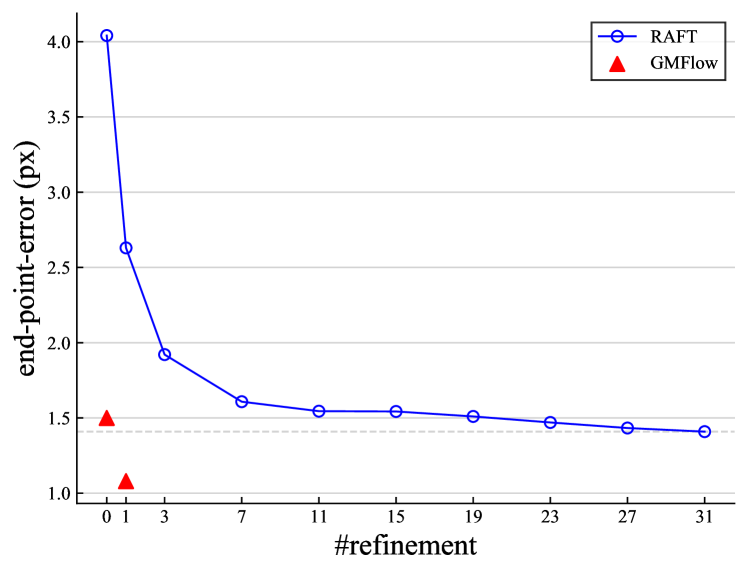
To alleviate the large displacements issue, RAFT [41] proposes an iterative framework with a large number of iterative refinements where convolutions are applied to different local cost volumes at different iteration stages so as to gradually reach near-global search space, achieving outstanding performance on standard benchmarks. The current state-of-the-art methods [19, 48, 53, 41] are all based on such an iterative architecture. Despite the excellent performance, such a large number of sequential refinements introduce linearly increasing inference time, which makes it hard for speed optimization and hinders its deployment in real-world applications. This raises a question: Is it possible to achieve both high accuracy and efficiency without requiring such a large number of iterative refinements?

We notice that another visual correspondence problem, i.e., sparse matching between an image pair [36, 45, 40], which usually features a large viewpoint change, moves into a different track. The top-performing sparse methods (e.g., SuperGlue [36] and LoFTR [40]) adopt Transformers [43] to reason about the mutual relationship between feature descriptors, and the correspondences are extracted with an explicit matching layer (e.g., softmax layer [45]).

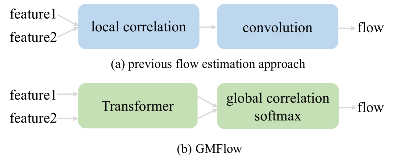
Inspired by sparse matching, we propose to completely remove the additional convolutional layers operating on a predefined local cost volume, and reformulate optical flow as a global matching problem, which is distinct from all previous learning-based optical flow methods. Fig. 1 provides a conceptual comparison of these two flow estimation approaches. Our flow prediction is obtained with a differentiable matching layer, i.e., correlation and softmax layer, by comparing feature similarities. Such a formulation calls for more discriminative feature representations, for which the Transformer [43] becomes a natural choice.

We would like to point out that although our pipeline shares the conceptual major components (i.e., Transfromer and the softmax matching layer) with sparse matching [36, 40], our motivation is originated from the development of optical flow methods and the challenges associated with formulating optical flow as a global matching problem are quite different. Optical flow focuses on dense correspondences for every pixel and modern learning-based architectures are mostly designed by regression from a local cost volume. The scale and complexity of optical flow are much higher. Moreover, optical flow needs to deal with occluded and out-of-boundary pixels, for which the simple softmax-based matching layer will not be effective.

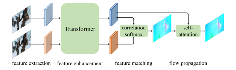
In this paper, we propose a GMFlow framework to realize the global matching formulation for optical flow. Specifically, the dense features extracted from a convolutional backbone network are fed into a Transformer that consists of self-, cross-attentions and feed-forward network to obtain more discriminative features. We then compare the feature similarities by correlating all pair-wise features. After that, the flow prediction is obtained with a differentiable softmax matching layer. To address occluded and out-of-boundary pixels, we incorporate an additional self-attention layer to propagate the high-quality flow prediction from matched pixels to unmatched ones by exploiting the feature self-similarity [15, 19]. We further introduce a refinement step that reuses GMFlow at higher feature resolution for residual flow prediction. Our full framework achieves competitive performance and higher efficiency compared with the state-of-the-art methods. Specifically, with only one refinement, GMFlow outperforms 31-refinements RAFT on the challenging Sintel [4] dataset, while running faster.

Our major contributions can be summarized as follows:

• We completely revamp the dominant flow regression pipeline by reformulating optical flow as a global matching problem, which effectively addresses the long-standing challenge of large displacements.

• We propose a GMFlow framework to realize the global matching formulation, which consists of three main components: a Transformer for feature enhancement, a correlation and softmax layer for global feature matching, and a self-attention layer for flow propagation.

• We further propose a refinement step to exploit higher resolution feature, which allows us to reuse the same GMFlow framework for residual flow estimation.

• GMFlow outperforms 31-refinements RAFT on the challenging Sintel benchmark, while using only one refinement and running faster, suggesting a new paradigm for accurate and efficient flow estimation.

Figure 2: Overview of GMFlow framework. We first extract $8\times$ downsampled dense features from two input video frames with a weight-sharing convolutional network. Then the features are fed into a Transformer for feature enhancement. Next we compare feature similarities by correlating all pair-wise features and the optical flow is obtained with a softmax matching layer. An additional self-attention layer is introduced to propagate the high-quality flow predictions in matched pixels to unmatched ones by considering the feature self-similarity.

2 Related Work

Flow estimation approach. The flow estimation approach is fundamental to existing popular optical flow frameworks [17, 38, 16, 41, 48, 19, 53], notably the coarse-to-fine method PWC-Net [38] and iterative refinement method RAFT [41]. They both perform some sort of multi-stage refinements, either at multiple scales [38] or a single resolution [41]. For flow prediction at each stage, their pipeline is conceptual similar, i.e., regressing optical flow from a local cost volume with convolutions. However, such an approach is hard to handle large displacements. Thus multi-stage refinements are required to estimate large motion incrementally. The success of RAFT largely lies in the large number of iterative refinements it can perform. Two exceptions to these local regression approaches are DICL [44] and GLU-Net [42]. DICL performs local matching with convolutions, while GLU-Net regresses flow from global correlation with convolutions, which also makes itself restricted to fixed image resolution and thus an additional sub-network is required to handle this issue. Distinct from these approaches, we perform global matching with a Transformer and we show it is indeed possible to achieve highly accurate results without relying on a large number of refinements.

Large displacements. Large displacements have been a long-standing challenge for optical flow [2, 47, 3, 7, 1]. One popular strategy is to use the coarse-to-fine approach [14, 3, 38] that estimates large motion incrementally. However, coarse-to-fine methods tend to miss fast-moving small objects [34] if the resolution is too coarse. To alleviate this issue, RAFT [41] proposes to maintain a single high resolution and gradually improve the initial prediction with a large number of iterative refinements, achieving remarkable performance on standard benchmarks. However, such a large number of sequential refinements introduce linearly increasing inference time, which makes it hard for speed optimization and hinders its integration into real-world systems. In contrast, our new framework streamlines the optical flow pipeline and estimates large displacements with both high accuracy and efficiency, achieved by a reformulation of the optical flow problem and a strong Transformer.

Transformer for correspondences. SuperGlue [36] pioneered the use of Transformer for sparse feature matching. LoFTR [40] further improves its performance by removing the feature detection step in the typical pipelines. COTR [20] formulates the correspondence problem as a functional mapping by querying the interest point and uses a Transformer as the function. These frameworks are mainly designed for sparse matching problems, and it is non-trivial to directly adopt them to dense correspondence tasks. Although COTR in principle can also predict dense correspondences by querying every pixel location, the inference speed will be significantly slower. For dense correspondences, STTR [24] is a Transformer-based method for stereo matching, which can be viewed as a special case of optical flow. Besides, STTR relies on a complex optimal transport matching layer and doesn’t produce predictions for occluded pixels, while we use a much simpler softmax operation and a simple flow propagation layer to handle occlusion. Another related work Perceiver IO [18] targets general problems and uses optical flow as an application in experiments. Although both method are based on Transformers, Perceiver IO directly regresses optical flow via self-attention, while we aim at learning strong feature representations (in particular with cross-attention) for matching.

3 Methodology

Optical flow is intuitively a matching problem that aims at finding corresponding pixels. To achieve this, one can compare the similarity of the features for each pixel, and identify the corresponding pixel that gives the highest similarity. Such a process requires the features to be discriminative enough to stand out. Aggregating the spatial contexts within the image itself and information from another image can intuitively alleviate ambiguities and improve their distinctiveness. Such design philosophies have enabled great achievement in sparse feature matching frameworks [36, 40]. The success of sparse matching, which usually features a large viewpoint change, motivates us to formulate optical flow as an explicit global matching problem in order to address the challenge of large displacements.

In the following, we first provide a general description of our global matching formulation, and then present a Transformer-based framework to realize it.

3.1 Formulation

Given two consecutive video frames ${\bm{I}}_{1}$ and ${\bm{I}}_{2}$, we first extract downsampled dense features ${\bm{F}}_{1},{\bm{F}}_{2}\in\mathbb{R}^{H\times W\times D}$ with a weight-sharing convolutional network, where $H,W$ and $D$ denote height, width and feature dimension, respectively. Considering the correspondences in the two frames should share high similarity, we first compare the feature similarity for each pixel in ${\bm{F}}_{1}$ with respect to all pixels in ${\bm{F}}_{2}$ by computing their correlations [45]. This can be implemented efficiently with a simple matrix multiplication:

$${\bm{C}}=\frac{{\bm{F}}_{1}{\bm{F}}_{2}^{T}}{\sqrt{D}}\in\mathbb{R}^{H\times W\times H\times W},$$ (1)

where each element in the correlation matrix ${\bm{C}}$ represents the correlation value between coordinates ${\bm{p}}_{1}=(i,j)$ in ${\bm{F}}_{1}$ and ${\bm{p}}_{2}=(k,l)$ in ${\bm{F}}_{2}$, and $\frac{1}{\sqrt{D}}$ is a normalization factor to avoid large values after the dot-product operation [43].

To identify the correspondence, one naïve approach is to directly take the location that gives the highest correlation. However, this operation is unfortunately non-differentiable, which prevents end-to-end training. To tackle this issue, we use a differentiable matching layer [45, 21, 49]. Specifically, we normalize the last two dimensions of ${\bm{C}}$ with the softmax operation, which gives us a matching distribution

$${\bm{M}}=\mathrm{softmax}({\bm{C}})\in\mathbb{R}^{H\times W\times H\times W}$$ (2)

for each location in ${\bm{F}}_{1}$ with respect to all locations in ${\bm{F}}_{2}$. Then, the correspondence $\hat{{\bm{G}}}$ can be obtained by taking a weighted average of the 2D coordinates of pixel grid ${\bm{G}}\in\mathbb{R}^{H\times W\times 2}$ with the matching distribution ${\bm{M}}$:

$$\hat{{\bm{G}}}={\bm{M}}{\bm{G}}\in\mathbb{R}^{H\times W\times 2}.$$ (3)

Finally, the optical flow ${\bm{V}}$ can be obtained by computing the difference between the corresponding pixel coordinates

$${\bm{V}}=\hat{{\bm{G}}}-{\bm{G}}\in\mathbb{R}^{H\times W\times 2}.$$ (4)

Such a softmax-based approach can not only enable end-to-end training but also provide sub-pixel accuracy.

3.2 Feature Enhancement

Key to our formulation lies in obtaining high-quality discriminative features for matching. Recall that the features ${\bm{F}}_{1}$ and ${\bm{F}}_{2}$ in Sec. 3.1 are extracted independently from a weight-sharing convolutional network. To further consider their mutual dependencies, a natural choice is Transformer [43], which is particularly suitable for modeling the mutual relationship between two sets with the attention mechanism, as demonstrated in sparse matching methods [36, 40]. Since ${\bm{F}}_{1}$ and ${\bm{F}}_{2}$ are only two sets of features, they have no notion of the spatial position, we first add the fixed 2D sine and cosine positional encodings (following DETR [6]) to the features. Adding the position information also makes the matching process consider not only the feature similarity but also their spatial distance, which can help resolve ambiguities and improve the performance (Table LABEL:tab:transformer).

After adding the position information, we perform six stacked self-, cross-attentions and feed-forward network (FFN) [43] to improve the quality of the initial features. Specifically, for self-attention, the query, key and value in the attention mechanism [43] are the same feature. For cross-attention, the key and value are same but different from the query to introduce their mutual dependencies. This process is performed for both ${\bm{F}}_{1}$ and ${\bm{F}}_{2}$ symmetrically, i.e.,

$$\hat{\bm{F}}_{1}=\mathcal{T}({\bm{F}}_{1}+{\bm{P}},{\bm{F}}_{2}+{\bm{P}}),\hskip 6.00006pt\hat{\bm{F}}_{2}=\mathcal{T}({\bm{F}}_{2}+{\bm{P}},{\bm{F}}_{1}+{\bm{P}}),$$ (5)

where $\mathcal{T}$ is a Transformer, ${\bm{P}}$ is the positional encoding, the first input of $\mathcal{T}$ is query and the second is key and value.

One issue in the standard Transformer architecture [43] is the quadratic computational complexity due to the pair-wise attention operation. To improve the efficiency, we adopt the shifted local window attention strategy from Swin Transformer [26]. However, unlike Swin that uses fixed window size, we split the feature to fixed number of local windows to make the window size adaptive with the feature size. Specifically, we split the input feature of size $H\times W$ to $K\times K$ windows (each with size $\frac{H}{K}\times\frac{W}{K}$), and perform self- and cross-attentions within each local window independently. For every two consecutive local windows, we shift the window partition by $(\frac{H}{2K},\frac{W}{2K})$ to introduce cross-window connections. In our framework, we split to $2\times 2$ windows (each with size $\frac{H}{2}\times\frac{W}{2}$), which represents a good speed-accuracy trade-off (Table LABEL:tab:split_attn).

Figure 3: GMFlow also simplifies backward flow computation by transposing the global correlation matrix without requiring to forward the network twice. The bidirectional flow can be used for occlusion detection with forward-backward consistency check.

3.3 Flow Propagation

Our softmax-based flow estimation method implicitly assumes that the corresponding pixels are visible in both images and thus they can be matched by comparing their similarities. However, this assumption will be invalid for occluded and out-of-boundary pixels. To remedy this, by observing that the optical flow field and the image itself share high structure similarity [15, 19], we propose to propagate the high-quality flow predictions in matched pixels to unmatched ones by measuring the feature self-similarity. This operation can be implemented efficiently with a simple self-attention layer (illustrated in Fig. 2):

$$\tilde{\bm{V}}=\mathrm{softmax}\left(\frac{\hat{\bm{F}}_{1}\hat{\bm{F}_{1}}^{T}}{\sqrt{D}}\right)\hat{\bm{V}}\in\mathbb{R}^{H\times W\times 2},$$ (6)

where

$$\hat{\bm{V}}=\mathrm{softmax}\left(\frac{\hat{\bm{F}}_{1}\hat{\bm{F}_{2}}^{T}}{\sqrt{D}}\right){\bm{G}}-{\bm{G}},$$ (7)

is the optical flow prediction from the softmax layer, which is obtained by substituting the stronger features in Eq. (5) into the softmax matching layer in Sec. 3.1. Fig. 2 provides an overview of our GMFlow framework.

Method	#blocks	Things (val, clean)				Sintel (train, clean)				Sintel (train, final)				Param (M)
		EPE	$s_{0-10}$	$s_{10-40}$	$s_{40+}$	EPE	$s_{0-10}$	$s_{10-40}$	$s_{40+}$	EPE	$s_{0-10}$	$s_{10-40}$	$s_{40+}$
cost volume + conv	0	18.83	3.42	6.49	49.65	6.45	1.75	7.17	38.19	7.75	2.10	8.88	45.29	1.8
	4	10.99	1.70	3.41	29.78	3.32	0.73	3.84	20.58	4.93	0.99	5.71	31.16	4.6
	8	9.59	1.44	2.96	26.04	2.89	0.65	3.36	17.75	4.32	0.88	4.95	27.33	8.0
	12	9.04	1.37	2.84	24.46	2.78	0.65	3.32	16.69	4.07	0.84	4.76	25.44	11.5
	18	8.67	1.33	2.74	23.43	2.61	0.59	3.07	15.91	3.94	0.82	4.62	24.58	15.7
Transformer + softmax	0	22.93	8.57	11.13	52.07	8.44	2.71	11.60	42.10	10.28	3.11	13.83	53.34	1.0
	1	11.45	2.98	4.68	28.35	4.12	1.27	5.08	22.25	6.11	1.70	7.89	33.52	1.6
	2	8.59	1.80	3.28	21.99	3.09	0.90	3.66	17.37	4.54	1.24	5.44	26.00	2.1
	4	7.19	1.40	2.62	18.66	2.43	0.67	2.73	14.23	3.78	1.01	4.27	22.37	3.1
	6	6.67	1.26	2.40	17.37	2.28	0.58	2.49	13.89	3.44	0.80	3.97	21.02	4.2

Table 1: Methodology comparison. We stack different number of convolutional residual blocks or Transformer blocks to see how the performance varies. All models are trained on Chairs and Things training sets. We report the performance on Things validation clean set and the cross-dataset generalization results on Sintel training clean and final sets.

3.4 Refinement

The framework presented so far (based on $1/8$ features) can already achieve competitive performance (Table 3). It can be further improved by introducing additional higher resolution ($1/4$) feature for refinement. Specifically, we first upsample the previous $1/8$ flow prediction to $1/4$ resolution, and warp the second feature with the current flow prediction. Then the refinement task is reduced to the residual flow learning, where the same GMFlow framework depicted in Fig. 2 can be used but in a local range. Specifically, we split to $8\times 8$ local windows (each with $1/32$ of the original image resolution) in the Transformer and perform a $9\times 9$ local window matching for each pixel. After obtaining the flow prediction from the softmax layer, we perform a $3\times 3$ local window self-attention operation for flow propagation.

Note that here we share the Transformer and self-attention weights in the refinement step with the global matching stage, which not only reduces parameters but also improves the generalization (Table LABEL:tab:refine). To generate the $1/4$ and $1/8$ features, we also share the backbone features. Specifically, we take a similar approach to TridentNet [23] but use a weight-sharing convolution with strides $1$ and $2$, respectively. Such a weight-sharing design also leads to better performance than the feature pyramid network [25].

3.5 Training Loss

We supervise all flow predictions using $\ell_{1}$ loss between the ground truth:

$$L=\sum_{i=1}^{N}\gamma^{N-i}\|{\bm{V}}_{i}-{\bm{V}}_{\mathrm{gt}}\|_{1},$$ (8)

where $N$ is the number of flow predictions including the intermediate and final ones, and $\gamma$ (set to 0.9) is the weight that is exponentially increasing to give higher weights for later predictions following RAFT [41].

setup	Things (val)	Sintel (train)		Param (M)
	clean	clean	final
full	6.67	2.28	3.44	4.2
w/o cross	10.84	4.48	6.32	3.8
w/o pos	8.38	2.85	4.28	4.2
w/o FFN	8.71	3.10	4.43	1.8
w/o self	7.04	2.49	3.69	3.8

(a)

#splits	Things (val, clean)				Time (ms)
	EPE	$s_{0-10}$	$s_{10-40}$	$s_{40+}$
$1\times 1$	6.34	1.26	2.37	16.36	105
$2\times 2$	6.67	1.26	2.40	17.37	53
$4\times 4$	7.32	1.29	2.58	19.26	35

(b)

matching space	Things (val, clean)				Time (ms)
	EPE	$s_{0-10}$	$s_{10-40}$	$s_{40+}$
global	6.67	1.26	2.40	17.37	52.6
local $3\times 3$	31.78	1.19	12.40	85.39	51.2
local $5\times 5$	26.51	0.89	6.67	76.76	51.5
local $9\times 9$	19.88	1.01	2.44	61.06	52.9

(c)

prop.	Sintel (clean)			Sintel (final)
	all	matched	unmatched	all	matched	unmatched
w/o	2.28	1.06	15.54	3.44	1.95	19.50
w/	1.89	1.10	10.39	3.13	1.98	15.52

(d)

setup	share Trans?	share feature?	Things	Sintel (train)		Param (M)
			clean	clean	final
w/o refine	-	-	3.98	1.65	2.94	4.7
w/ refine			3.41	1.28	2.75	8.0
	✓		3.21	1.27	2.60	4.9
		✓	3.26	1.21	2.70	7.9
	✓	✓	3.24	1.20	2.59	4.7

(e)

training iterations	Things (val)	Sintel (train)		KITTI (train)
	clean	clean	final	EPE	F1-all
200K	3.24	1.20	2.59	9.32	26.95
400K	3.01	1.16	2.51	8.96	26.18
600K	2.93	1.13	2.42	8.34	24.77
800K	2.80	1.08	2.48	7.77	23.40

(f)

Table 2: GMFlow ablations. All models are trained on Chairs and Things training sets.

4 Experiments

Datasets and evaluation setup. Following previous methods [17, 38, 41], we first train on the FlyingChairs (Chairs) [10] and FlyingThings3D (Things) [29] datasets, and then evaluate Sintel [4] and KITTI [31] training sets. We also evaluate on the Things validation set to see how the model performs on the same-domain data. Finally, we perform additional fine-tuning on Sintel and KITTI training sets and report the performance on the online benchmarks.

Metrics. We adopt the commonly used metric in optical flow, i.e., the end-point-error (EPE), which is the average $\ell_{2}$ distance between the prediction and ground truth. For KITTI dataset, we also use F1-all, which reflects the percentage of outliers. To better understand the performance gains, we also report the EPE in different motion magnitudes. Specifically, we use $s_{0-10},s_{10-40}$ and $s_{40+}$, to denote the EPE over pixels with ground truth flow motion magnitude falling to $0-10$, $10-40$ and more than $40$ pixels.

Implementation details. We implement our framework in PyTorch. Our convolutional backbone network is identical to RAFT’s model, except that our final feature dimension is 128, while RAFT’s is 256. We stack 6 Transformer blocks. To upsample the low-resolution flow prediction to the original image resolution, we use RAFT’s convex upsampling [41] method. We use AdamW [27] as the optimizer. We first train the model on Chairs dataset for 100K iterations, with a batch size of 16 and a learning rate of 4e-4. We then fine-tune it on Things dataset for 200K iterations for ablation experiments, with a batch size of 8 and a learning rate of 2e-4. Our best model is fine-tuned on Things for 800K iterations. For the final fine-tuning process on Sintel and KITTI datasets, we report the details in Sec. 4.4. Further details are provided in the supplementary material.

4.1 Methodology Comparison

Flow estimation approach. We compare our Transformer and softmax-based flow estimation method with the cost volume and convolution-based approach. Specifically, we adopt the state-of-the-art cost volume construction method in RAFT [41] that concatenates 4 local cost volumes at 4 scales, where each cost volume has a dimension of $H\times W\times(2R+1)^{2}$, where $H$ and $W$ are image height and width, respectively, and the search range $R$ is set to 4 following RAFT. To regress flow, we stack different number of convolutional residual blocks [12] to see how the performance varies. The final optical flow is obtained with a $3\times 3$ convolution with 2 output channels. For our proposed framework, we stack different number of Transformer blocks for feature enhancement, where one Transformer block consists of self-, cross-attentions and a feed-forward network (FFN). The final optical flow is obtained with a global correlation and softmax layer. Both methods use bilinear upsampling in this comparison. Table 1 shows that the performance improvement of our method is more significant compared to the cost volume and convolution-based approach. For instance, our method with 2 Transformer blocks can already outperform 8 convolution blocks, especially for large motion ($s_{40+}$). The performance can be further improved by stacking more layers, surpassing the cost volume and convolution-based approach by a large margin. We present more comparisons with all the possible combinations of different flow estimation approaches in the supplementary material, where our method is consistently better and has less parameters than other variants.

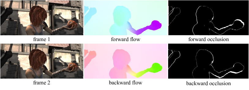
Bidirectional flow prediction. Our framework also simplifies backward optical flow computation by directly transposing the global correlation matrix in Eq. (1). Note that during training we only predict unidirectional flow while at inference we can obtain bidirectional flow for free, without requiring to forward the network twice, unlike previous regression-based methods [30, 16]. The bidirectional flow can be used for occlusion detection with forward-backward consistency check (following [30]), as shown in Fig. 3.

Method	#refine.	Things (val, clean)				Sintel (train, clean)				Sintel (train, final)				Param (M)	Time (ms)
		EPE	$s_{0-10}$	$s_{10-40}$	$s_{40+}$	EPE	$s_{0-10}$	$s_{10-40}$	$s_{40+}$	EPE	$s_{0-10}$	$s_{10-40}$	$s_{40+}$
RAFT [41]	0	14.28	1.47	3.62	40.48	4.04	0.77	4.30	26.66	5.45	0.99	6.30	35.19	5.3	25 (14)
	3	6.27	0.69	1.67	17.63	1.92	0.47	2.32	11.37	3.25	0.65	4.00	20.04		39 (21)
	7	4.66	0.55	1.38	12.87	1.61	0.39	1.90	9.61	2.80	0.53	3.30	17.76		58 (31)
	11	4.31	0.53	1.33	11.79	1.55	0.41	1.73	9.19	2.72	0.52	3.12	17.43		78 (41)
	23	4.22	0.53	1.32	11.52	1.47	0.36	1.63	9.00	2.69	0.52	3.05	17.28		133 (71)
	31	4.25	0.53	1.31	11.63	1.41	0.32	1.55	8.83	2.69	0.52	3.00	17.45		170 (91)
GMFlow	0	3.48	0.67	1.31	8.97	1.50	0.46	1.77	8.26	2.96	0.72	3.45	17.70	4.7	57 (26)
	1	2.80	0.53	1.01	7.31	1.08	0.30	1.25	6.26	2.48	0.51	2.81	15.67	4.7	151 (66)

Table 3: RAFT’s iterative refinement framework vs. our GMFlow framework. The models are trained on Chairs and Things training sets. We use RAFT’s officially released model for evaluation. The inference time is measured on a single V100 and A100 (in parentheses) GPU at Sintel resolution ($436\times 1024$). Our framework gains more speedup than RAFT ($2.29\times$ vs. $1.87\times$, i.e., ours: $151\to 66$, RAFT: $170\to 91$) on the high-end A100 GPU since our method doesn’t require a large number of sequential computation.

4.2 Ablations

Transformer components. We ablate different Transformer components in Table LABEL:tab:transformer. The cross-attention contributes most, since it models the mutual relationship between two features, which is missing in the features extracted from the convolutional backbone network. Also, the position information makes the matching process position-dependent, and can be conducive to alleviate the ambiguities in pure feature similarity-based matching. Removing the feed-forward network (FFN) reduces a large number of parameters, while also leading to a moderate performance drop. The self-attention aggregates contextual cues within the same feature, bringing additional performance gains.

Figure 4: Optical flow end-point-error vs. number of refinements at inference time. This figure shows the generalization results on Sintel (clean) training set after training on Chairs and Things datasets. Our method outperforms 31-refinements RAFT’s performance while using only one refinement and running faster.

Local window attention. We compare the speed-accuracy trade-off of splitting to different numbers of local windows for attention computation in Table LABEL:tab:split_attn. Recall that the extracted features from backbone is $1/8$ resolution, further splitting to $H/2\times W/2$ local windows (i.e., $1/16$ of the original resolution) represents a good trade-off between accuracy and speed, and thus is used in our framework.

Matching Space. We replace our global matching with local matching in Table LABEL:tab:global_local_match and observe a significant performance drop, especially for large motion ($s_{40+}$). Besides, the global matching can be computed efficiently with a simple matrix multiplication, while larger size for local matching will be slower due to the excessive sampling operation.

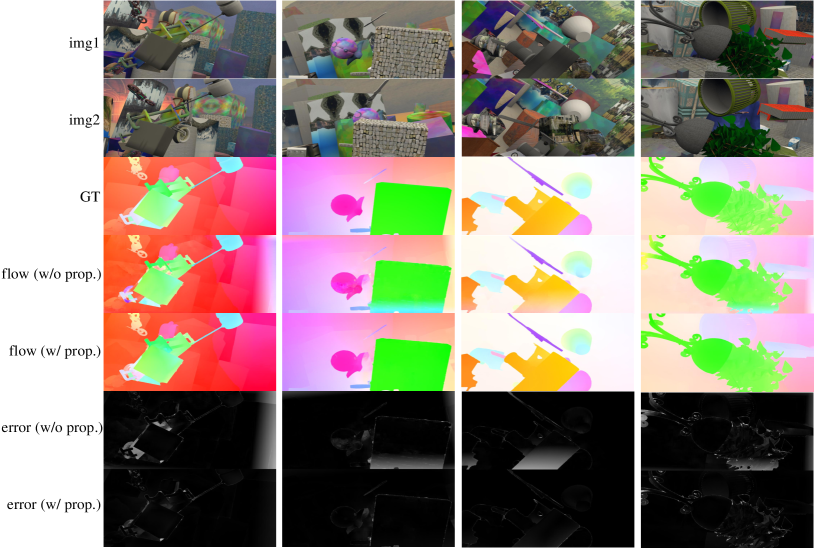
Flow propagation. Our flow propagation strategy results in significant performance gains in unmatched regions (including occluded and out-of-boundary pixels), as shown in Table LABEL:tab:prop. The structural correlation between the feature and flow provides a valuable clue to improve the performance of pixels that are challenging to match. Visual comparisons are provided in the supplementary material.

Refinement. We compare whether to share the backbone when extracting $1/8$ and $1/4$ features, and whether to share the Transformer for matching at $1/8$ and $1/4$ resolutions. The results are shown in Table LABEL:tab:refine. Sharing Transformer and multi-scale features better regularizes the learning process, leading to better performance and less parameters.

Training length. Our ablations thus far are based on 200K-iterations fine-tuning on Things dataset. In Table LABEL:tab:train_schedule, we show our framework benefits from more training iterations, consistent with the observations in previous vision Transformer works [9, 26]. We use 800K-iterations model as our final model in subsequent comparisons.

We analyze the computational complexities of core components in our framework in the supplementary material.

Training data	Method	EPE	F1-all	$s_{0-10}$	$s_{10-40}$	$s_{40+}$
C + T	RAFT	5.32	17.46	0.67	1.58	13.68
	GMFlow	7.77	23.40	0.74	2.19	20.34
C + T + VK	RAFT	2.45	7.90	0.43	1.18	5.70
	GMFlow	2.85	10.77	0.49	1.16	6.87

Table 4: Generalization on KITTI after training on synthetic Chairs (C), Things (T) and Virtual KITTI 2 (VK) datasets.

Figure 5: Visual comparisons on Sintel test set.

4.3 Comparison with RAFT

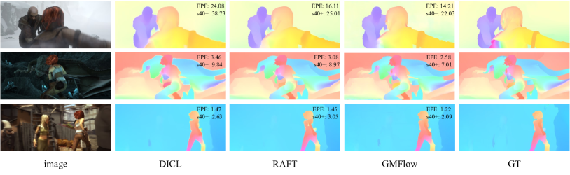
Sintel. Table 3 shows the results on Things validation set and Sintel clean and final training sets after training on Chairs and Things training sets. Without using any refinement, our method achieves better performance on Things and Sintel (clean) than RAFT with 11 refinements. By using an additional refinement, our method outperforms RAFT with 31 refinements, especially on large motion ($s_{40+}$). Fig. 4 visualizes the results. Furthermore, our framework enjoys faster inference speed compared to RAFT and also does not require a large number of sequential processing. On the high-end A100 GPU, our framework gains more speedup compared with RAFT’s sequential framework ($2.29\times$ vs. $1.87\times$, i.e., ours: $151\to 66$, RAFT: $170\to 91$), reflecting that our framework can benefit more from advanced hardware acceleration and showing its potential for further speed optimization.

KITTI. Table 4 shows the generalization results on KITTI training set after training on Chairs and Things training sets. In this evaluation setting, our framework doesn’t outperform RAFT, which is mainly caused by the gap between the synthetic training sets and the real-world testing dataset. One key reason behind our inferior performance is that RAFT, relying on fully convolutional neural networks, benefits from the inductive biases in convolution layers, which requires a relatively smaller size training data to generalize to a new dataset in comparison with Transformers [9, 8, 50, 54]. To substantiate this claim, we fine-tune both RAFT and our method on the additional Virtual KITTI 2 [5] dataset. We can see from Table 4 that the performance gap becomes smaller when more data is available.

Method	Sintel (clean)			Sintel (final)
	all	matched	unmatched	all	matched	unmatched
FlowNet2 [17]	4.16	1.56	25.40	5.74	2.75	30.11
PWC-Net+ [39]	3.45	1.41	20.12	4.60	2.25	23.70
HD3 [52]	4.79	1.62	30.63	4.67	2.17	24.99
VCN [51]	2.81	1.11	16.68	4.40	2.22	22.24
DICL [44]	2.63	0.97	16.24	3.60	1.66	19.44
RAFT [41]	1.94	-	-	3.18	-	-
GMFlow	1.74	0.65	10.56	2.90	1.32	15.80
RAFT† [41]	1.61	0.62	9.65	2.86	1.41	14.68
GMA† [19]	1.39	0.58	7.96	2.47	1.24	12.50

Table 5: Comparisons on Sintel test test. ^† represents the method uses last frame’s flow prediction as initialization for subsequent refinement, while other methods all use two frames only.

4.4 Comparison on Benchmarks

Sintel. Following previous works [41, 48], we further fine-tune our Things model on several mixed datasets that consist of KITTI [31], HD1K [22], FlyingThings3D [29] and Sintel [4] training sets. We perform fine-tuning for 200K iterations with a batch size of 8 and a learning rate of 2e-4. The results on Sintel test set are shown in Table 5. We achieve best performance among all the competitive state-of-the-art methods that only use two frames at inference. Although RAFT can also use last frame’s prediction as initialization for subsequent refinement, we still achieve comparable performance in matched regions even without using multi-frame information. Qualitative comparisons between GMFlow and other state-of-the-art approaches on Sintel test set are shown in Fig. 5. More visual results on DAVIS [32] dataset are given in the supplementary material.

KITTI. We perform additional fine-tuning on the KITTI 2015 training set from the model trained on Sintel. We train GMFlow for 100K iterations with a batch size of 8 and a learning rate of 2e-4. Table 6 shows the evaluation results. For non-occluded (Noc) pixels, our performance is slightly inferior to RAFT. For all pixels that contain both non-occluded and occluded pixels, the performance gap becomes larger, which indicates that our inferior performance largely lies in occluded regions.

Method	FlowNet2 [17]	PWC-Net+ [39]	RAFT [41]	GMFlow
All	11.48	7.72	5.10	9.32
Noc	6.94	4.91	3.07	3.80

Table 6: Comparisons on KITTI test set. The metric is F1-all. “All” denotes the evaluation results on all pixels with ground truth, and “Noc” denotes non-occluded pixels only.

4.5 Limitation and Discussion

Our framework still has room for future improvement in occluded regions, as can be seen from the KITTI results in Table 6. Besides, our framework may not generalize very well when the training data has significantly large gap with the test data (e.g., synthetic Things to real-world KITTI). Fortunately, there are many large-scale datasets available currently, e.g., Virtual KITTI [11, 5], VIPER [35], REFRESH [28], AutoFlow [37] and TartanAir [46], they can be used to enhance Transformer’s generalization ability.

5 Conclusion

We have presented a new global matching formulation for optical flow and demonstrated its strong performance. We hope our new perspective will pave a way towards a new paradigm for accurate and efficient optical flow estimation.

Broader impact. Our proposed method might produce unreliable results in occluded regions, thus care should be taken when using the prediction results from our model, especially for safety-critical scenarios like self-driving cars.

Acknowledgement. This research is supported in part by Monash FIT Start-up Grant. Dr. Jing Zhang is supported by ARC FL-170100117.

Appendix

A More Comparisons

We present more comprehensive comparisons (as a supplement of Table 1 in the main paper) with all the possible combinations of flow estimation approaches in Table A. Our Transformer and softmax-based method is consistently better and has less parameters than other variants.

Method	feature enhancement	flow prediction	#convs	Sintel (train, clean)			Sintel (train, final)			Param (M)
				all	matched	unmatched	all	matched	unmatched
variants	-	cost + conv	14	3.32	1.56	22.34	4.93	2.82	27.73	4.64
	Transformer	cost + conv	2	3.41	2.40	14.32	4.57	3.27	18.67	4.95
	Transformer	cost + conv	14	2.04	1.09	12.34	3.37	2.03	17.80	7.79
	conv	softmax	14	6.36	3.22	40.30	8.00	4.80	42.58	5.12
GMFlow (w/o prop.)	Transformer	softmax	0	2.28	1.06	15.54	3.44	1.95	19.50	4.20
GMFlow (w/ prop.)	Transformer	softmax	0	1.89	1.10	10.39	3.13	1.98	15.52	4.23

Table A: Comparisons on different variants of flow estimation approaches. Although the Transformer can also be used for feature enhancement in the cost volume and convolution-based approach (cost + conv), its performance heavily relies on a deep convolutional regressor (e.g., 14 layers to catch up). In contrast, our softmax-based method is parameter-free (4.20M vs. 7.79M). The flow propagation (prop.) layer further improves ours performance in unmatched regions, while only introducing additional 0.03M parameters. Replacing the Transformer with convolutions for feature enhancement leads to significantly large performance drop, since convolutions are not able to model the mutual relationship between two features.

B Computational Complexity

We analyze the computational complexities of core components in our framework below.

Global Matching. In our global matching formulation, we build a 4D correlation matrix $H\times W\times H\times W$ to model all pair-wise similarities between two features (with size $H\times W$, $1/8$ of the original image resolution). There exists an equivalent implementation should it become a bottleneck for high-resolution images. Note that the pixels in the first feature are independent and thus their flow predictions can be computed sequentially. Specifically, we can sequentially compute $K\times K$ correlation matrices (each with size $H/K\times W/K\times H\times W$), and finally merge the results for all pixels. Such a sequential implementation can save the memory consumption while having little influence on the overall inference time (see Table B), since the global matching operation only needs to compute once, and it’s not a significant speed bottleneck in the full framework.

#splits	$1\times 1$	$2\times 2$	$4\times 4$	$8\times 8$
Time (ms)	52.57	52.64	52.90	59.45

Table B: Inference time vs. number of splits for sequential global matching implementation. The input image resolution is $448\times 1024$, and the features are downsampled by $8\times$.

Transformer. We use shifted local window attention [26] in the Transformer implementation, where each local window size is $1/16$ of the original image resolution by default. The computational cost is usually acceptable for regular image resolutions (e.g., $448\times 1024$). Note that we can always switch to smaller windows size (e.g., $1/32$, see Table LABEL:tab:split_attn of the main paper) should it become a bottleneck.

Flow Propagation. Our default flow propagation scheme computes a global self-attention. The sequential implementation in global matching can also be adopted here. It’s also possible to compute a local window self-attention only for less memory consumption by trading some accuracy in large motion (Table C). Such a local attention operation can be implemented efficiently with PyTorch’s unfold function.

self-attn.	Sintel (train, final)
	EPE	$s_{0-10}$	$s_{10-40}$	$s_{40+}$
global	3.13	0.80	3.87	18.04
local $3\times 3$	3.31	0.79	3.75	20.22
local $5\times 5$	3.21	0.75	3.66	19.69

Table C: Global vs. local self-attention for flow propagation.

Refinement. Although the feature resolution of our refinement architecture is higher ($1/4$), it is not a significant bottleneck since smaller local window ($1/32$ of the original image resolution) attention is used in the Transformer and matching is performed within a local window.

Overall, our GMFlow framework is general and flexible, and many concrete implementations are possible to meet specific needs.

C More Visual Results

Flow Propagation. Our flow propagation scheme with self-attention is quite effective for handling occluded and out-of-boundary pixels, as can be seen from Fig. A.

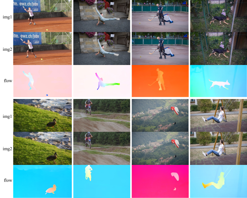
Prediction on DAVIS dataset. We test our pre-trained Sintel model on the DAVIS [32] dataset, the results on diverse scenes are shown in Fig. B.

Figure A: Our flow propagation (prop.) scheme significantly improves the performance of occluded and out-of-boundary pixels.

Figure B: Visual results on DAVIS dataset.

D More Implementation Details

Network Architectures. The Transformer feature dimension is 128, and the intermediate feed-forward network expands the dimension by $4\times$. We only use a single head in all the attention computations, since we observe that multi-head attention slows down the speed without bringing obvious performance gains. Our refinement architecture uses exactly the same Transformer for feature enhancement, except that the attentions are performed within smaller local windows. The self-attention layer in the flow propagation step is also shared for $1/8$ and $1/4$ resolutions, where we perform global attention at $1/8$ resolution and local $3\times 3$ window attention at $1/4$ resolution.

Training Details. Our data augmentation strategy mostly follows RAFT [41] except that we didn’t use occlusion augmentation, since no obvious improvement is observed in our experiments. During training, we perform random cropping following previous works. The crop size for FlyingChairs is $384\times 512$, FlyingThings3D is $384\times 768$, Sintel is $320\times 896$ and KITTI is $320\times 1152$. Our framework without refinement is trained on 4 V100 (16GB) GPUs. The full framework with refinement is trained on 4 A100 (40GB) GPUs. We are also able to reproduce the results on 4 V100 (16GB) GPUs by halving the batch size and doubling the training iterations.

References

- [1] Christian Bailer, Bertram Taetz, and Didier Stricker. Flow fields: Dense correspondence fields for highly accurate large displacement optical flow estimation. In ICCV, pages 4015–4023, 2015.
- [2] Thomas Brox, Christoph Bregler, and Jitendra Malik. Large displacement optical flow. In ICCV, pages 41–48. IEEE, 2009.
- [3] Thomas Brox, Andrés Bruhn, Nils Papenberg, and Joachim Weickert. High accuracy optical flow estimation based on a theory for warping. In ECCV, pages 25–36. Springer, 2004.
- [4] Daniel J Butler, Jonas Wulff, Garrett B Stanley, and Michael J Black. A naturalistic open source movie for optical flow evaluation. In ECCV, pages 611–625. Springer, 2012.
- [5] Yohann Cabon, Naila Murray, and Martin Humenberger. Virtual kitti 2. arXiv preprint arXiv:2001.10773, 2020.
- [6] Nicolas Carion, Francisco Massa, Gabriel Synnaeve, Nicolas Usunier, Alexander Kirillov, and Sergey Zagoruyko. End-to-end object detection with transformers. In ECCV, pages 213–229. Springer, 2020.
- [7] Zhuoyuan Chen, Hailin Jin, Zhe Lin, Scott Cohen, and Ying Wu. Large displacement optical flow from nearest neighbor fields. In CVPR, pages 2443–2450, 2013.
- [8] Stéphane d’Ascoli, Hugo Touvron, Matthew Leavitt, Ari Morcos, Giulio Biroli, and Levent Sagun. Convit: Improving vision transformers with soft convolutional inductive biases. ICML, 2021.
- [9] Alexey Dosovitskiy, Lucas Beyer, Alexander Kolesnikov, Dirk Weissenborn, Xiaohua Zhai, Thomas Unterthiner, Mostafa Dehghani, Matthias Minderer, Georg Heigold, Sylvain Gelly, Jakob Uszkoreit, and Neil Houlsby. An image is worth 16x16 words: Transformers for image recognition at scale. ICLR, 2021.
- [10] Alexey Dosovitskiy, Philipp Fischer, Eddy Ilg, Philip Hausser, Caner Hazirbas, Vladimir Golkov, Patrick Van Der Smagt, Daniel Cremers, and Thomas Brox. Flownet: Learning optical flow with convolutional networks. In ICCV, pages 2758–2766, 2015.
- [11] Adrien Gaidon, Qiao Wang, Yohann Cabon, and Eleonora Vig. Virtual worlds as proxy for multi-object tracking analysis. In CVPR, pages 4340–4349, 2016.
- [12] Kaiming He, Xiangyu Zhang, Shaoqing Ren, and Jian Sun. Deep residual learning for image recognition. In CVPR, pages 770–778, 2016.
- [13] Asmaa Hosni, Christoph Rhemann, Michael Bleyer, Carsten Rother, and Margrit Gelautz. Fast cost-volume filtering for visual correspondence and beyond. TPAMI, 35(2):504–511, 2012.
- [14] Yinlin Hu, Rui Song, and Yunsong Li. Efficient coarse-to-fine patchmatch for large displacement optical flow. In CVPR, pages 5704–5712, 2016.
- [15] Tak-Wai Hui and Chen Change Loy. Liteflownet3: Resolving correspondence ambiguity for more accurate optical flow estimation. In ECCV, pages 169–184. Springer, 2020.
- [16] Junhwa Hur and Stefan Roth. Iterative residual refinement for joint optical flow and occlusion estimation. In CVPR, pages 5754–5763, 2019.
- [17] Eddy Ilg, Nikolaus Mayer, Tonmoy Saikia, Margret Keuper, Alexey Dosovitskiy, and Thomas Brox. Flownet 2.0: Evolution of optical flow estimation with deep networks. In CVPR, pages 2462–2470, 2017.
- [18] Andrew Jaegle, Sebastian Borgeaud, Jean-Baptiste Alayrac, Carl Doersch, Catalin Ionescu, David Ding, Skanda Koppula, Daniel Zoran, Andrew Brock, Evan Shelhamer, et al. Perceiver io: A general architecture for structured inputs & outputs. In ICLR, 2022.
- [19] Shihao Jiang, Dylan Campbell, Yao Lu, Hongdong Li, and Richard Hartley. Learning to estimate hidden motions with global motion aggregation. In ICCV, pages 9772–9781, October 2021.
- [20] Wei Jiang, Eduard Trulls, Jan Hosang, Andrea Tagliasacchi, and Kwang Moo Yi. Cotr: Correspondence transformer for matching across images. ICCV, 2021.
- [21] Alex Kendall, Hayk Martirosyan, Saumitro Dasgupta, Peter Henry, Ryan Kennedy, Abraham Bachrach, and Adam Bry. End-to-end learning of geometry and context for deep stereo regression. In ICCV, pages 66–75, 2017.
- [22] Daniel Kondermann, Rahul Nair, Katrin Honauer, Karsten Krispin, Jonas Andrulis, Alexander Brock, Burkhard Gussefeld, Mohsen Rahimimoghaddam, Sabine Hofmann, Claus Brenner, et al. The hci benchmark suite: Stereo and flow ground truth with uncertainties for urban autonomous driving. In CVPR Workshops, pages 19–28, 2016.
- [23] Yanghao Li, Yuntao Chen, Naiyan Wang, and Zhaoxiang Zhang. Scale-aware trident networks for object detection. In ICCV, pages 6054–6063, 2019.
- [24] Zhaoshuo Li, Xingtong Liu, Nathan Drenkow, Andy Ding, Francis X Creighton, Russell H Taylor, and Mathias Unberath. Revisiting stereo depth estimation from a sequence-to-sequence perspective with transformers. In ICCV, pages 6197–6206, 2021.
- [25] Tsung-Yi Lin, Piotr Dollár, Ross Girshick, Kaiming He, Bharath Hariharan, and Serge Belongie. Feature pyramid networks for object detection. In CVPR, pages 2117–2125, 2017.
- [26] Ze Liu, Yutong Lin, Yue Cao, Han Hu, Yixuan Wei, Zheng Zhang, Stephen Lin, and Baining Guo. Swin transformer: Hierarchical vision transformer using shifted windows. ICCV, 2021.
- [27] Ilya Loshchilov and Frank Hutter. Decoupled weight decay regularization. arXiv preprint arXiv:1711.05101, 2017.
- [28] Zhaoyang Lv, Kihwan Kim, Alejandro Troccoli, Deqing Sun, James M Rehg, and Jan Kautz. Learning rigidity in dynamic scenes with a moving camera for 3d motion field estimation. In ECCV, pages 468–484, 2018.
- [29] Nikolaus Mayer, Eddy Ilg, Philip Hausser, Philipp Fischer, Daniel Cremers, Alexey Dosovitskiy, and Thomas Brox. A large dataset to train convolutional networks for disparity, optical flow, and scene flow estimation. In CVPR, pages 4040–4048, 2016.
- [30] Simon Meister, Junhwa Hur, and Stefan Roth. Unflow: Unsupervised learning of optical flow with a bidirectional census loss. In AAAI, 2018.
- [31] Moritz Menze and Andreas Geiger. Object scene flow for autonomous vehicles. In CVPR, pages 3061–3070, 2015.
- [32] Federico Perazzi, Jordi Pont-Tuset, Brian McWilliams, Luc Van Gool, Markus Gross, and Alexander Sorkine-Hornung. A benchmark dataset and evaluation methodology for video object segmentation. In CVPR, pages 724–732, 2016.
- [33] Anurag Ranjan and Michael J Black. Optical flow estimation using a spatial pyramid network. In CVPR, pages 4161–4170, 2017.
- [34] Jerome Revaud, Philippe Weinzaepfel, Zaid Harchaoui, and Cordelia Schmid. Epicflow: Edge-preserving interpolation of correspondences for optical flow. In CVPR, pages 1164–1172, 2015.
- [35] Stephan R Richter, Zeeshan Hayder, and Vladlen Koltun. Playing for benchmarks. In ICCV, pages 2213–2222, 2017.
- [36] Paul-Edouard Sarlin, Daniel DeTone, Tomasz Malisiewicz, and Andrew Rabinovich. Superglue: Learning feature matching with graph neural networks. In CVPR, pages 4938–4947, 2020.
- [37] Deqing Sun, Daniel Vlasic, Charles Herrmann, Varun Jampani, Michael Krainin, Huiwen Chang, Ramin Zabih, William T Freeman, and Ce Liu. Autoflow: Learning a better training set for optical flow. In CVPR, pages 10093–10102, 2021.
- [38] Deqing Sun, Xiaodong Yang, Ming-Yu Liu, and Jan Kautz. Pwc-net: Cnns for optical flow using pyramid, warping, and cost volume. In CVPR, pages 8934–8943, 2018.
- [39] Deqing Sun, Xiaodong Yang, Ming-Yu Liu, and Jan Kautz. Models matter, so does training: An empirical study of cnns for optical flow estimation. TPAMI, 42(6):1408–1423, 2019.
- [40] Jiaming Sun, Zehong Shen, Yuang Wang, Hujun Bao, and Xiaowei Zhou. Loftr: Detector-free local feature matching with transformers. In CVPR, pages 8922–8931, 2021.
- [41] Zachary Teed and Jia Deng. Raft: Recurrent all-pairs field transforms for optical flow. In ECCV, pages 402–419. Springer, 2020.
- [42] Prune Truong, Martin Danelljan, and Radu Timofte. Glu-net: Global-local universal network for dense flow and correspondences. In CVPR, pages 6258–6268, 2020.
- [43] Ashish Vaswani, Noam Shazeer, Niki Parmar, Jakob Uszkoreit, Llion Jones, Aidan N Gomez, Łukasz Kaiser, and Illia Polosukhin. Attention is all you need. In NeurIPS, pages 5998–6008, 2017.
- [44] Jianyuan Wang, Yiran Zhong, Yuchao Dai, Kaihao Zhang, Pan Ji, and Hongdong Li. Displacement-invariant matching cost learning for accurate optical flow estimation. NeurIPS, 33, 2020.
- [45] Qianqian Wang, Xiaowei Zhou, Bharath Hariharan, and Noah Snavely. Learning feature descriptors using camera pose supervision. In ECCV, pages 757–774. Springer, 2020.
- [46] Wenshan Wang, Delong Zhu, Xiangwei Wang, Yaoyu Hu, Yuheng Qiu, Chen Wang, Yafei Hu, Ashish Kapoor, and Sebastian Scherer. Tartanair: A dataset to push the limits of visual slam. 2020.
- [47] Philippe Weinzaepfel, Jerome Revaud, Zaid Harchaoui, and Cordelia Schmid. Deepflow: Large displacement optical flow with deep matching. In ICCV, pages 1385–1392, 2013.
- [48] Haofei Xu, Jiaolong Yang, Jianfei Cai, Juyong Zhang, and Xin Tong. High-resolution optical flow from 1d attention and correlation. In ICCV, pages 10498–10507, 2021.
- [49] Haofei Xu and Juyong Zhang. Aanet: Adaptive aggregation network for efficient stereo matching. In CVPR, pages 1959–1968, 2020.
- [50] Yufei Xu, Qiming Zhang, Jing Zhang, and Dacheng Tao. Vitae: Vision transformer advanced by exploring intrinsic inductive bias. NeurIPS, 2021.
- [51] Gengshan Yang and Deva Ramanan. Volumetric correspondence networks for optical flow. NeurIPS, 32:794–805, 2019.
- [52] Zhichao Yin, Trevor Darrell, and Fisher Yu. Hierarchical discrete distribution decomposition for match density estimation. In CVPR, pages 6044–6053, 2019.
- [53] Feihu Zhang, Oliver J. Woodford, Victor Adrian Prisacariu, and Philip H.S. Torr. Separable flow: Learning motion cost volumes for optical flow estimation. In ICCV, pages 10807–10817, October 2021.
- [54] Qiming Zhang, Yufei Xu, Jing Zhang, and Dacheng Tao. Vitaev2: Vision transformer advanced by exploring inductive bias for image recognition and beyond. arXiv preprint arXiv:2202.10108, 2022.