SWAT: Spatial Structure Within and Among Tokens

Abstract

Modeling visual data as tokens (i.e., image patches) using attention mechanisms, feed-forward networks or convolutions has been highly effective in recent years. Such methods usually have a common pipeline: a tokenization method, followed by a set of layers/blocks for information mixing, both within and among tokens. When image patches are converted into tokens, they are often flattened, discarding the spatial structure within each patch. As a result, any processing that follows (eg: multi-head self-attention) may fail to recover and/or benefit from such information. In this paper, we argue that models can have significant gains when spatial structure is preserved during tokenization, and is explicitly used during the mixing stage. We propose two key contributions: (1) Structure-aware Tokenization and, (2) Structure-aware Mixing, both of which can be combined with existing models with minimal effort. We introduce a family of models (SWAT), showing improvements over the likes of DeiT, MLP-Mixer and Swin Transformer, across multiple benchmarks including ImageNet classification and ADE20K segmentation. Our code is available at github.com/kkahatapitiya/SWAT.

1 Introduction

Convolutional architectures (CNNs) He et al. (2016) have been dominant in computer vision for a while now. When they were first introduced for large-scale training in image domain, their benefits were quickly realized over Multi-layer Perceptrons (MLPs). In addition to efficient weight sharing, the inductive bias generated by exploring the local structure in images was one of the key factors for its success LeCun et al. (2015). In language domain however, CNNs were less effective due to lack of such strong local structure. Consequently, attention mechanisms emerged dominant, exploring long-range relationships and modeling language as a sequence Dauphin et al. (2017). More recently, attention models– specifically Transformers Vaswani et al. (2017), have been extended to represent visual data Dosovitskiy et al. (2021), with the key concept of tokenizing an input image to create a sequence (or a set), often discarding their structure. Within a short period of time, such token-based models (i.e., class of models such as ViTs Dosovitskiy et al. (2021) and MLP-Mixers Tolstikhin et al. (2021)) have outperformed CNNs on most visual tasks. However, we ask, could the spatial structure– when preserved, benefit token-based models and further improve their performance?

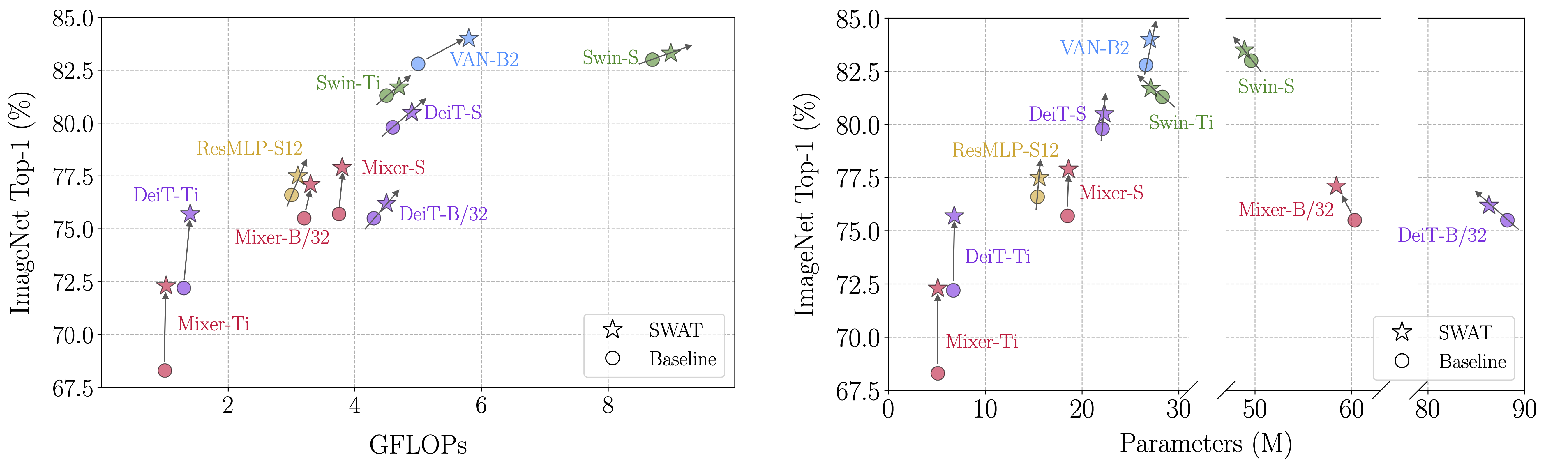
Figure 1: Performance vs. Complexity on ImageNet-1K Deng et al. (2009). We implement our proposed (1) Structure-aware Tokenization, and (2) Structure-aware Mixing in common token-based architectures including DeiT Touvron et al. (2021b), Swin Liu et al. (2021), MLP-Mixer Tolstikhin et al. (2021), ResMLP Touvron et al. (2021a) and VAN Guo et al. (2022). The resulting family of SWAT models consistently outperform their counterparts, with minimal increase in complexity. We consider the system-agnostic metrics such as FLOPs and Parameters as the complexity measures here.

Token-based models in computer vision are rapidly evolving. From Vision Transformers Dosovitskiy et al. (2021) to MLP-Mixers Tolstikhin et al. (2021) and hybrid-architectures Peng et al. (2021); Wu et al. (2021), intriguing concepts are being introduced and tested on tasks including classification Dosovitskiy et al. (2021); Touvron et al. (2021b); Liu et al. (2021), detection Zhu et al. (2020); Dai et al. (2021) and segmentation Xie et al. (2021); Duke et al. (2021), to name a few. All such models can be framed with two main components: (1) Tokenization, which converts image patches into tokens, and (2) Mixing (attention-based as in Multi-head Self Attention (MHSA), MLP-based or convolution-based), which shares information within and among tokens. In general, during tokenization, an image patch is directly mapped into a token, not preserving the spatial structure within a token. After this mapping, models usually focus on global patterns among tokens, without capturing local spatial structure within tokens.

Structure is an important cue in visual data. In images, 2D spatial structure preserves geometry and object-part relationships. Simply put, structure gives meaning to visual data in human perspective. However, in machine perspective, if a jumbled set of image patches are tokenized and processed through a token-based model, it can give the same classification performance (as it is a set operator), even though the input is really meaningless to a human Naseer et al. (2021). This is in fact a drawback of token-based models (eg: can be prone to such an adversarial attack), which could be addressed by structure-aware modeling. Not only the structure among tokens, but also the structure within tokens is equally-important which is often discarded during tokenization. It is particularly beneficial to maintain the structure within tokens for fine-grained prediction tasks such as segmentation.

In this paper, we propose to preserve and make use of the spatial structure both within and among tokens. To do this we focus on two components: (1) Structure-aware Tokenization and (2) Structure-aware Mixing, both of which can be adopted in existing token-based architectures with minimal effort. Our Structure-aware Tokenization converts image patches to tokens, but preserves the spatial structure within a patch as channel segments of the corresponding token. Our Structure-aware Mixing benefits from the preserved structure by considering local neighborhoods both within and among tokens, based on 2D convolutions. We also refer to this as token mixing with channel structure and channel mixing with token structure. With these two contributions, we introduce a family of models: SWAT, and compare against common baselines such as DeiT Touvron et al. (2021b), Swin Transformer Liu et al. (2021), MLP-Mixer Tolstikhin et al. (2021), ResMLP Touvron et al. (2021a) and VAN Guo et al. (2022). Our models show consistent improvements over baseline models on multiple benchmarks including ImageNet-1K Deng et al. (2009) classification and ADE20K Zhou et al. (2019) semantic segmentation. We further visualize fine-grained attention patterns captured by our structure-aware modeling. Performance gains on ImageNet-1K classification against complexity (measured by system-agnostic metrics such as FLOPs and Parameters) are shown in Fig. 1.

2 Related Work

Token-based models:

Transformer architectures from language domain Vaswani et al. (2017); Devlin et al. (2019) have been recently adopted to visual data in the seminal work ViT Dosovitskiy et al. (2021). Even though attention mechanisms already existed in computer vision Wang et al. (2018); Zhao et al. (2020), their true potential was realized when introduced with tokenization. Since then, a variety of token-based models have been introduced, some with the use of MLPs Tolstikhin et al. (2021); Touvron et al. (2021a) or convolutions Trockman and Kolter (2022); Liu et al. (2022). DeiT Touvron et al. (2021b) introduces an efficient training recipe, and Caron et al. (2021); Ranasinghe et al. (2022) use self-supervision. Swin Transformer Liu et al. (2021) introduces attention within shifted-windows, while downsampling progressively similar to Heo et al. (2021); Wang et al. (2021); Fan et al. (2021). Another direction explores efficiency of such models Zhai et al. (2021); Bello (2020); Graham et al. (2021); Tang et al. (2021); Yue et al. (2021); Ryoo et al. (2021).

Token adoption in vision tasks:

Token-based models are already applied in most vision applications, including classification Touvron et al. (2021b); Liu et al. (2021), object detection Zhu et al. (2020); Carion et al. (2020), segmentation Xie et al. (2021); Duke et al. (2021), image generation Cao et al. (2021); Esser et al. (2021), video understanding Nagrani et al. (2021); Fan et al. (2021); Arnab et al. (2021); Dai et al. (2022), dense prediction Yang et al. (2021a); Ranftl et al. (2021), point clouds processing Zhao et al. (2021); Guo et al. (2021) and reinforcement learning Chen et al. (2021a); Shang et al. (2022).

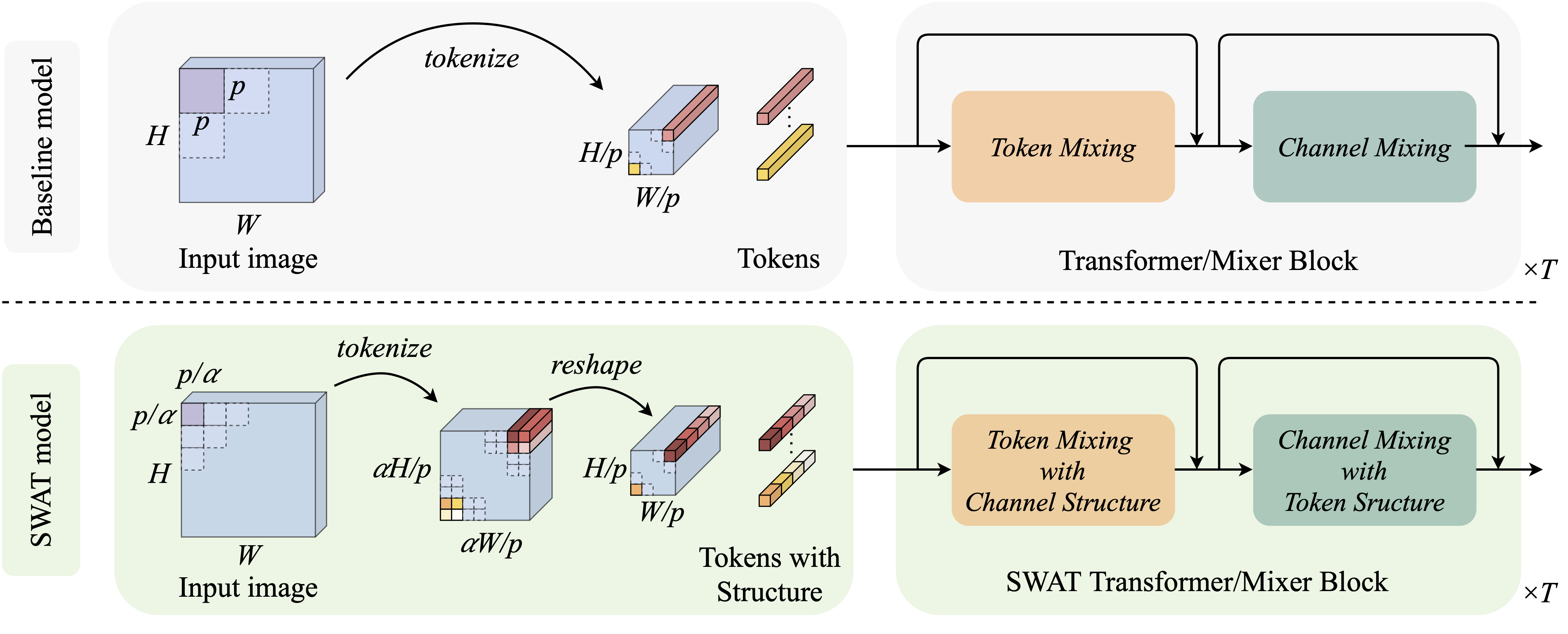
Figure 2: SWAT Overview: We show the architecture of SWAT (bottom) and a baseline model (top) in this figure. We propose two main contributions: (1) Structure-aware Tokenization and, (2) Structure-aware Mixing, which can be applied to common Transformer or Mixer architectures with minimal effort. Structure-aware tokenization preserves the spatial structure within a token, as channel segments. Simply put, first, we tokenize with a patch size $(p/\alpha\times p/\alpha)$ instead of $(p\times p)$, resulting in $\times\alpha^{2}$ more intermediate tokens. Next, we restructure $\alpha\times\alpha$ neighboring tokens into one token (concatenating in channel dimension), which gives the same number of tokens (and the channel dimension) into Mixing operations, ensuring no additional cost in the downstream. However, now, this newly-preserved structure within tokens can be explored for better downstream processing, which was very limited previously. More on how we use the structure in Mixing is shown in Fig. 3 and Fig. 4.

Structure with token-based models:

Some prior work in token-based models have explored structure, using hybrid architectures with convolutions Xiao et al. (2021); Peng et al. (2021); d’Ascoli et al. (2021). A structure-based grouping method is proposed in T2T-ViT Yuan et al. (2021b). With a complementary motivation to ours, TNT Han et al. (2021) and NesT Zhang et al. (2021) both consider a sub-token structure within tokens, but introduce additional tokens and become heavier with extra processing. Yuan et al. (2021a) has similarities with our channel mixing with token structure. Models such as ConvMixer Trockman and Kolter (2022), ConvNeXt Liu et al. (2022) and VAN Guo et al. (2022) also consider a convolutional design as ours (w/ Pointwise Conv and Depthwise Conv). However, they only consider structure among tokens, not structure within tokens. To our knowledge, this is the first work to preserve structure within tokens, without extra tokens or processing, i.e., with a minimal change in footprint.

3 Spatial Structure Within and Among Tokens

In SWAT family of models, we explore the benefits of preserving spatial structure not only among tokens, but within tokens as well. To do this with a general framework, we consider all token-based models (eg: ViTs Dosovitskiy et al. (2021), Mixers Tolstikhin et al. (2021)) as a unified architecture, which consists of two main components: (1) Tokenization, for converting image patches into tokens, and, (2) Mixing, for sharing information within and among tokens. Mixing can mean either the use of Multi-Layer Perceptron (MLP), Multi-Headed Self-Attention (MHSA) or convolution for information sharing. In this framework, we suggest improvements to both Tokenization and Mixing. When these components are adopted together in a network, it can preserve and utilize the spatial structure. Namely, we introduce Structure-aware Tokenization and Structure-aware Mixing, which we describe below in detail.

3.1 Structure-aware Tokenization

Here, we propose to preserve the spatial structure within tokens, not imposing any additional burden on downstream processing. The idea is to keep spatial information within tokens separated as its channel segments, so that the ‘mixing’ component can later take advantage of it. In general, image patches are converted into tokens by sliding a large convolutional kernel with a stride (eg: a $16\times 16$ kernel with a stride of 16), which extracts a set of tokens. In such a setting, all the spatial information within a patch is directly fused into the channels of the corresponding token, losing the explicit structure in the process. In our method, we replace this direct fusion, retaining structural information within tokens.

More concretely, let us consider an input image of size $H\times W\times 3$, and a baseline tokenizer which converts image patches into tokens by extracting non-overlapping patches of size $p\times p$. This is usually implemented as a convolutional layer with $C$ kernels of size $(p\times p)$, applied at a stride of $p$. The output here will be an $H/p\times W/p$ 2D structure of tokens, which is reshaped to create a sequence of $HW/p^{2}$ tokens of embedding dimension $C$ (refer Fig. 2 top). Even though these tokens are processed downstream as a sequence, they can be reshaped back into the original 2D structure of $H/p\times W/p$ whenever necessary. It has been observed that the tokens preserve this structure (among tokens) through skip connections and positional encodings Caron et al. (2021); Naseer et al. (2021), even after a series of Mixing blocks. However, the structure within a $p\times p$ patch is irreversibly lost, i.e., although each token is a linear abstraction of $p\times p$ pixels, remapping the token back to its original $p\times p$ shape in subsequent layers is not directly feasible.

In contrast, the proposed tokenizer in SWAT retains the structure within a token (refer Fig. 2 bottom). We do this by first having $C/\alpha^{2}$ convolutional kernels of size $(p/\alpha\times p/\alpha)$ (where $\alpha>1$) and applying it with a stride of $p/\alpha$. The resulting intermediate set of tokens will have a 2D structure of $\alpha H/p\times\alpha W/p$ and a dimension of $C/\alpha^{2}$. Next, such $\alpha\times\alpha$ neighboring tokens are reshaped into a single token (concatenating in the channel dimension), creating the same number of tokens $HW/p^{2}$ as the baseline, with the embedding dimension of $C$. By doing so, we now have an $\alpha\times\alpha$ 2D structure within each token– as its channel segments, which can be preserved throughout downstream processing, by the same principles: skip connections and (optional) positional embeddings. Note that the SWAT tokenizer will have a fewer parameters, in fact, $3Cp^{2}/\alpha^{4}$, compared to that of the baseline ($3Cp^{2}$), which can impair the learning capacity. To avoid this in practice, we use a bottleneck structure of multiple layers instead of a single convolution layer (still having the same downsampling factor of $1/\alpha$ as the baseline), which will enable the tokenizer to have an equivalent capacity, while introducing structure within tokens.

3.2 Structure-aware Mixing

To make use of the structured tokens (w/ spatial structure both within and among) generated by the SWAT tokenizer, we propose Structure-aware Mixing. The idea is straightforward: when we have such a 2D structure, the corresponding elements (either tokens or channels) will have the notion of neighboring elements in the 2D space, which gives an inductive bias that we can benefit from. Our approach uses this locality in a form of 2D convolutions, mixing information in a local region of elements, in addition to the usual global information sharing in Transformer/Mixer models. We present this idea in two parts: (1) Token Mixing with Channel Structure and, (2) Channel Mixing with Token Structure.

3.2.1 Token Mixing with Channel Structure

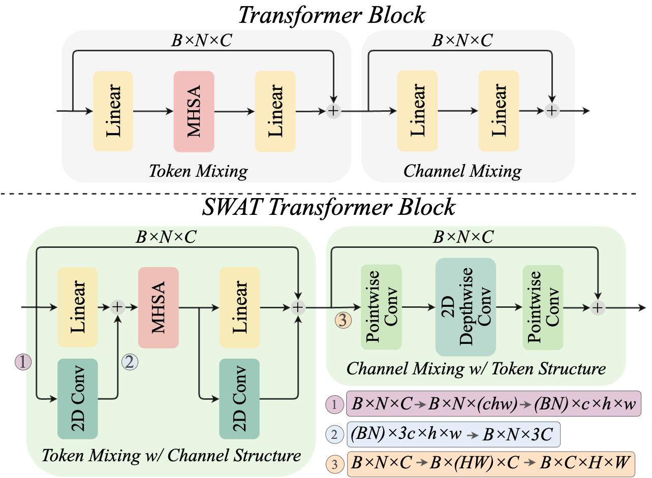
Figure 3: SWAT Transformer Block: We benefit from 2D channel structure (within tokens) in token mixing, and 2D token structure (among tokens) in channel mixing: (1) We insert a 2D Conv in-parallel to each Linear projection in attention (MHSA) block, applied on a reshaped input. It explicitly considers a structured local neighborhood within a token during token mixing. (2) In channel mixing, we first replace Linear layers with Pointwise Conv as a design decision for implementation simplicity. Next, we insert a 2D Depthwise Conv to consider a structured local neighborhood among tokens. Key tensor reshape operations are highlighted.

Token Mixing happens in different ways in Transformers Dosovitskiy et al. (2021); Touvron et al. (2021b) and Mixers Tolstikhin et al. (2021); Touvron et al. (2021a). In Transformers, each token attends to every other token pairwise and dynamically (w/ input-dependent weights). In an attention block, a MHSA layer is sandwiched between two Linear projection layers. Here, by design, token mixing (i.e., information sharing among tokens) happens while also mixing channels. These Linear layers may reshuffle channels and waste our newly-introduced structure within tokens, as there is not even a skip-connection to save it. In contrast, in Mixers, token mixing is done with static relations (w/ learned weights), while not reshuffling channels. Simply put, tokens are mixed channel-wise, without damaging the structure within tokens. Therefore, we follow different designs in Transformers and Mixers to introduce our token mixing with channel structure.

Figure 4: SWAT Mixer Block: In both token mixing and channel mixing, we first replace Linear layers with Pointwise Conv, applied on a reshaped input (eg: a Linear layer on a ($B\times N\times C$) shaped tensor equals to a Pointwise Conv on ($B\times C\times N$), in a PyTorch-like channel-first Conv implementation). This is a design decision for implementation simplicity, which makes no change in how an input is processed. Now, we can easily explore the 2D channel structure (within tokens) in token mixing and, 2D token structure (among tokens) in channel mixing, by inserting a 2D Depthwise Conv. Key tensor reshape operations are highlighted.

Transformers:

We insert a 2D Conv in-parallel to the Linear layers before and after MHSA, to explore the channel structure (structure within tokens). See Fig. 3 bottom-left. After SWAT tokenizer, the channel dimension $C$ has an internal structure of $c\times h\times w$ (as in Fig. 2, with usual notation), which we use to reshape the input as,

$$B\times N\times C\rightarrow B\times N\times(chw)\rightarrow(BN)\times c\times h\times w.$$

Here, $B$ represents batch, $N$, num. of tokens and $C$, embedding dimension. When a 2D Conv is applied on this tensor, it can mix channel information similar to a Linear layer, but also considering the inductive bias of channel structure.

Mixers:

In Mixers, we first replace the two Linear layers in token mixing with Pointwise $1\times 1$ Conv. See Fig. 4 bottom-left. We do this just to simplify the implementation, w/o changing the underlying operation (i.e., Linear = $1\times 1$ Conv). Applying a Linear layer on a tensor of shape $B\times C\times N$ is the same as applying a Pointwise Conv on a tensor $B\times N\times C$ (again, we consider a PyTorch-like implementation of channel-first Conv and channel-last Linear). Now, we can conveniently consider the 2D structure in channels (within tokens). Next, we insert a 2D Depthwise Conv in-between the Pointwise Conv layers, applied on a reshaped input as,

$$B\times N\times C\rightarrow B\times N\times(chw)\rightarrow(Bc)\times N\times h\times w.$$

Altogether, this token mixing block now considers the channel structure (i.e., structure within tokens).

3.2.2 Channel Mixing with Token Structure

Channel Mixing operation is the same for both Transformers and Mixers. In a baseline, two Linear layers are applied on an input tensor shaped as $B\times N\times C$ to mix channel information. In SWAT, we wish to do this while considering the token structure. Hence, we replace the two Linear layers with the same sandwich block: 2D Depthwise Conv in-between two Pointwise Conv, applied on an input reshaped as,

$$B\times N\times C\rightarrow B\times(HW)\times C\rightarrow B\times C\times H\times W.$$

See Fig. 3 or Fig. 4 bottom-right. This channel mixing block now considers token structure (i.e., structure among tokens).

Specific hyperparameter settings and ablations related to (1) newly-introduced structure within tokens, and (2) level of structure-awareness in mixing, are included in Appendix. When experimenting with pyramid architectures (eg: Swin), we need to explicitly preserve structure when downsampling, and how we do this is also described in Appendix.

4 Experiments

In this section, we evaluate our family of models, SWAT on image classification and semantic segmentation. We use Imagenet-1K Deng et al. (2009) and ADE20K Zhou et al. (2019) as benchmarks to compare against common Transformer/Mixer/Conv architectures such as DeiT Touvron et al. (2021b), Swin Liu et al. (2021), MLP-Mixer Tolstikhin et al. (2021), ResMLP Touvron et al. (2021a) and VAN Guo et al. (2022). In our ablations, we further evaluate the benefits of preserving structure.

4.1 ImageNet Classification

ImageNet-1K Deng et al. (2009) is a commonly-used classification benchmark, with 1.2M training images and 50K validation images, annotated with 1000 categories. For all our models, we report Top-1 (%) accuracy on single-crop evaluation with complexity metrics such as Parameters and FLOPs. We train all our models for 300 epochs on inputs of $224\times 224$ using the timm Wightman (2019) library. We use the original hyperparameters for all backbones, without further tuning. All models are trained with Mixed Precision.

Model	Model	Top-1	Params.	FLOPs
	scale	(%)	(M)	(G)
DeiT (Touvron et al.)	Ti	72.2	5.7	1.3
	S	79.8	22.1	4.6
	B/32	75.5	88.2	4.3
	Ti	(+3.5) 75.7	5.8	1.4
	S	(+0.7) 80.5	22.3	4.9
SWAT${}_{\text{DeiT}}$ (ours)	B/32	(+0.7) 76.2	86.3	4.5
Mixer (Tolstikhin et al.)	Ti	68.3	5.1	1.0
	S	75.7	18.5	3.8
	B/32	75.5	60.3	3.2
	Ti	(+4.0) 72.3	5.1	1.0
	S	(+2.2) 77.9	18.6	3.8
SWAT${}_{\text{Mixer}}$ (ours)	B/32	(+1.6) 77.1	58.4	3.3
Swin (Liu et al.)	Ti	81.3	28.3	4.5
	S	83.0	49.6	8.7
	Ti	(+0.4) 81.7	27.1	4.7
SWAT${}_{\text{Swin}}$ (ours)	S	(+0.3) 83.3	48.9	9.1

Table 1: SWAT is generally-applicable and scalable. We compare SWAT with DeiT Touvron et al. (2021b), MLP-Mixer Tolstikhin et al. (2021) and Swin Liu et al. (2021) on ImageNet-1K. We report the performance in Tiny, Small and Base/32 (i.e., patch size of 32$\times$32) configurations. SWAT models consistently outperform their counterparts with minimal change in parameters or computations. All models are trained for 300 epochs at $224\times 224$ resolution. Performance improvement is in bold.

Model		Top-1	Params.	FLOPs
		(%)	(M)	(G)
CNN	ResNet (He et al.)	78.8	25.6	4.1
	ResNeXt* (Xie et al.)	77.6	25.0	4.3
	EfficientNet* (Tan and Le)	82.6	19.3	4.4
	RegNetY* (Radosavovic et al.)	79.4	20.6	4.0
	ConvMixer (Trockman and Kolter)	80.2	21.1	-
	ConvNeXt (Liu et al.)	82.1	29.0	4.5
MLP	Mixer (Tolstikhin et al.)	75.7	18.5	3.8
	SWAT${}_{\text{Mixer}}$ (ours)	(+2.2) 77.9	18.6	3.8
	gMLP (Touvron et al.)	79.6	20.0	4.5
	ResMLP* (Touvron et al.)	76.6	15.4	3.0
	SWAT${}_{\text{ResMLP}}$* (ours)	(+1.2) 77.8	15.6	3.1
	PoolFormer (Yu et al.)	80.3	21.4	3.6
	CycleMLP (Chen et al.)	81.6	27.0	3.9
Attention	DeiT (Touvron et al.)	79.8	22.1	4.6
	SWAT${}_{\text{DeiT}}$ (ours)	(+0.7) 80.5	22.3	4.9
	T2T-ViT (Yuan et al.)	81.5	21.5	4.8
	TNT (Han et al.)	81.5	23.8	5.2
	NesT (Zhang et al.)	81.5	17.0	5.8
	PVT (Wang et al.)	79.8	24.5	3.8
	Twins (Chu et al.)	81.7	24.0	2.8
	Focal (Yang et al.)	82.2	29.1	4.9
	Swin (Liu et al.)	81.3	28.3	4.5
	SWAT${}_{\text{Swin}}$ (ours)	(+0.4) 81.7	27.1	4.7
Hybrid	ConViT (d’Ascoli et al.)	81.3	27.0	5.4
	CvT (Wu et al.)	81.6	20.0	4.5
	Conformer (Peng et al.)	81.3	23.5	5.2
	CeiT (Yuan et al.)	82.0	24.2	4.8
	MobileFormer* (Chen et al.)	79.3	14.0	0.5
	VAN (Guo et al.)	82.8	26.6	5.0
	SWAT${}_{\text{VAN}}$ (ours)	(+0.6) 83.4	27.0	5.8

Table 2: SWAT is competitive with SOTA. We report experiments on ImageNet-1K with different families of token-based models in mid-sized configurations (14-30M params.). We implement SWAT with DeiT Touvron et al. (2021b), Swin Liu et al. (2021), MLP-Mixer Tolstikhin et al. (2021), ResMLP Touvron et al. (2021a) and VAN Guo et al. (2022) baselines, and train with original hyperparameter settings. SWAT outperforms all baselines consistently with minimal change in complexity, showing competitive performance with SOTA models. In general, models are trained for 300 epochs at $224\times 224$ resolution (exceptions denoted with ^∗ are discussed in appendix). Performance improvement is in bold.

SWAT is generally-applicable and scalable:

In Table 1, we present the performance of SWAT with the two main types of token-based models: those using attention (MHSA) such as DeiT Touvron et al. (2021b) and Swin Liu et al. (2021), or those using MLPs such as Mixer Tolstikhin et al. (2021). In both model families, SWAT consistently outperforms the baselines across different model scales, verifying that our Structure-aware Tokenization and Structure-aware Mixing can be applied in both cases. Specifically, we consider Tiny, Small and Base/32 (i.e., patch size of 32$\times$32) model scales, with varying range of parameters and computations. These are standard models reported in previous work. We implement our tokenizer and replace Transformer/Mixing blocks with ours in each configuration (eg: DeiT-Ti $\rightarrow$ SWAT${}_{\text{DeiT}}$-Ti). In all configurations, SWAT models show consistent improvements. In SWAT${}_{\text{DeiT}}$, Tiny version achieves the highest gain of $+3.5\%$, with $+0.7\%$ in Small and Base/32. In SWAT${}_{\text{Mixer}}$, all Tiny ($+4.0\%$), Small ($+2.2\%$) and Base/32 ($+1.6\%$) versions show a considerable improvement over baselines. SWAT${}_{\text{Swin}}$ shows $+0.4\%$ w/ Tiny and $+0.3\%$ w/ Small models. Overall, SWAT models have minimal (or no) increment in parameters or computations. The performance vs. complexity graphs are shown in Fig. 1.

SWAT is competitive with SOTA:

In Table 2, we implement SWAT with multiple families of token-based models, either Transformer/Mixer/Convolutional, including DeiT Touvron et al. (2021b), Swin Liu et al. (2021), Mixer Tolstikhin et al. (2021), ResMLP Touvron et al. (2021a) and VAN Guo et al. (2022). We report the performance in mid-sized (14-30M parameters) standard configurations. We use the same hyperparameter settings and training recipes as the corresponding original baselines. We observe consistent gains in SWAT family of models: $+2.2\%$ in SWAT${}_{\text{Mixer}}$ and $+1.2\%$ in SWAT${}_{\text{ResMLP}}$, $+0.7\%$ in SWAT${}_{\text{DeiT}}$, $+0.4\%$ in SWAT${}_{\text{Swin}}$ and $+0.6\%$ in SWAT${}_{\text{VAN}}$, with minimal change in parameters and computations compared to baselines. This further shows that SWAT can be generally-adopted to any token-based architecture with minimal effort and cost.

SWAT shows more fine-grained attention patterns:

In Fig. 5, we visualize token attention values in Tiny configurations of DeiT Touvron et al. (2021b) and SWAT${}_{\text{DeiT}}$. We use the code from DINO Caron et al. (2021) paper as a base. However, in our models, since we do not use a class token, we cannot visualize the attention on a single token as in Caron et al. (2021). Instead, we show the attention maps of the final layer of each model, averaged across tokens. We consider larger image size ($1024\times 1024$) compared to training ($224\times 224$) to get higher resolution visualizations. We use the same patch size of 16 and interpolate positional encodings accordingly. We can see clear differences between the attention in DeiT Touvron et al. (2021b) and SWAT${}_{\text{DeiT}}$. In SWAT, we have more contrastive attention which resembles fine-grained structures (eg: boundaries in object segments), since we preserve such structure within tokens. In contrast, DeiT attention is smoothed-out and subtle. Also, the attention weights in the SWAT model are less-noisy. We use the same resolution (i.e., same number of tokens) in both cases.

We include a detailed analysis of model throughput (im/s) in SWAT models and their baselines at inference, in the Appedix. We consider FLOPs and parameters as our metrics of complexity, as they are system-agnostic and reproducible.

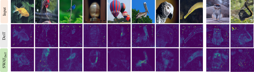
Figure 5: Visualization of token attention in DeiT-Ti Touvron et al. (2021b) and SWAT${}_{\text{DeiT}}$-Ti. We use the code from DINO Caron et al. (2021) for visualization. However since we do not use class tokens as in DINO, we show the attention averaged across tokens. SWAT, as it preserves structure even within tokens, shows more contrastive and fine-grained attention maps compared to DeiT (even though we consider same number of tokens, i.e., resolution, in both). Note the better-visible boundaries and segments in SWAT, compared to smoothed-out variations in DeiT. Some cases where SWAT fails to capture fine details are also shown (to the right). Best viewed in color and zoomed-in.

4.2 Ablations on ImageNet

Model	Structure-aware			Top-1	Params.	FLOPs
	Tokenize	Tk. Mix.	Ch. Mix.	(%)	(M)	(G)
DeiT				73.3	5.72	1.25
			✓	74.6	5.96	1.30
		✓		73.7	5.72	1.30
	✓			73.0	5.58	1.30
	✓	✓		74.5	5.59	1.35
SWAT${}_{\text{DeiT}}$	✓	✓	✓	75.7	5.83	1.40
Mixer				68.3	5.07	0.97
			✓	70.8	5.28	1.01
		✓		68.9	5.08	0.97
	✓			67.9	4.88	0.94
	✓	✓		70.2	4.88	0.95
SWAT${}_{\text{Mixer}}$	✓	✓	✓	72.3	5.10	0.99

Table 3: Ablations on Structure with DeiT-Ti Touvron et al. (2021b) and Mixer-Ti Tolstikhin et al. (2021) on ImageNet-1K. We report the gains from (1) Structure-aware Tokenization, (2) Token Mixing with Channel Structure, and (3) Channel Mixing with Token Structure. Structure-aware inputs and Structure-aware Mixing gives consistent improvements, as shown in bold. A key observation: our Tokenization and our Token Mixing should always be coupled.

In this section, We present ablations on Tiny versions of SWAT${}_{\text{DeiT}}$ and SWAT${}_{\text{Mixer}}$. Specifically, in Table 3, we focus on Structure-aware Tokenization, Token Mixing with Channel Structure and Channel Mixing with Token Structure.

Structure-aware Tokenization:

We compare different settings with SWAT tokenizer. Bottom line is that Structure-aware Tokenization should always be coupled with the Structure-aware Token Mixing. It makes sense: if we prepare tokens with structure and not take advantage of it during mixing, it does not really have a benefit and the reduced capacity (due to our Tokenization) may even drop the performance. In DeiT Touvron et al. (2021b), we see such performance drop of $-0.3\%$ when we do not use the structure (within tokens) explicitly. In Mixer Tolstikhin et al. (2021), this drop is $-0.4\%$. In both cases, when we specifically make use of the newly-introduced structure within tokens, we see consistent gains ($+1.5\%$ in DeiT and $+2.3\%$ in Mixer) over our Tokenization-only versions.

Channel Structure (within tokens) in Token Mixing:

Here, we intend to consider a local neighborhood within tokens. Even if such a structure is not present (i.e., not having our Tokenization), models can benefit slightly: $+0.4\%$ in DeiT Touvron et al. (2021b) and $+0.6\%$ in Mixer Tolstikhin et al. (2021). This is due to the inductive bias of replacing Linear layers with Conv. However, the true potential of this comes when a structure within tokens is explicitly available, where we see a $+1.2\%$ improvement in DeiT Touvron et al. (2021b) and $+1.9\%$ in Mixer Tolstikhin et al. (2021).

Token Structure (among tokens) in Channel Mixing:

Here, we consider a local neighborhood among tokens. In DeiT Touvron et al. (2021b), we see $+1.3\%$ boost, and in Mixer Tolstikhin et al. (2021), a $+2.5\%$ boost in performance.

4.3 Semantic Segmentation

ADE20K Zhou et al. (2019) benchmark contains annotations for semantic segmentation across 150 categories. It comes with 25K annotated images in total, with 20K training, 2K validation and 3K testing. We report mIoU for our models in multi-scale testing (i.e., [0.5, 0.75, 1.0, 1.25, 1.5, 1.75]$\times$ the training resolution) similar to previous work Liu et al. (2021), along with complexity metrics such as parameters, FLOPs (for input size of $512\times 2048$ similar to Liu et al. (2021)) and frame-rate. We follow a similar training recipe to Swin Liu et al. (2021). Our backbones are pretrained on ImageNet-1K Deng et al. (2009) for 300 epochs at $224\times 224$, before re-training with a decoder for segmentation at $512\times 512$. We use UperNet Xiao et al. (2018) as our decoder within mmsegmentation OpenMMLab (2020) framework. We use the original hyperparameter settings as the baseline.

Method	Backbone	mIoU	Params.	FLOPs	FPS
			(M)	(G)
DANet (Fu et al.)	Resnet-101 (He et al.)	45.2	69	1119	15.2
DLab.v3+ (Chen et al.)		44.1	63	1021	16.0
ACNet (Fu et al.)		45.9	-	-	-
DNL (Yin et al.)		46.0	69	1249	14.8
OCRNet (Yuan et al.)		45.3	56	923	19.3
UperNet (Xiao et al.)		44.9	86	1029	20.1
	DeiT-S (Touvron et al.)	44.0	52	1099	16.2
	Swin-Ti (Liu et al.)	45.8	60	945	18.5
	SWAT${}_{\text{Swin}}$-Ti (ours)	46.5	59	950	16.9
	VAN-B2 (Guo et al.)	50.1	57	948	-
UperNet (Xiao et al.)	SWAT${}_{\text{VAN}}$-B2 (ours)	50.7	55	952	-

Table 4: SWAT for semantic segmentation on ADE20K Zhou et al. (2019) dataset. We report results in the same setting as Swin Liu et al. (2021) using mmsegmentation OpenMMLab (2020) framework. FPS is measured on a single V100 GPU. SWAT outperforms respective baselines, but is slightly slower due to extra convolutions.

Results:

In Table 4, we show the performance of SWAT${}_{\text{Swin}}$ and SWAT${}_{\text{VAN}}$ backbones when used with the UperNet Xiao et al. (2018) head for semantic segmentation on ADE20K, and compare with similar-sized baselines. SWAT${}_{\text{Swin}}$ gives $+0.7$ mIoU and SWAT${}_{\text{VAN}}$ gives $+0.6$ mIoU improvement over the respective baselines, when trained under the same settings. However, FPS of the SWAT${}_{\text{Swin}}$ based model is slightly lower, due to extra convolutions introduced in SWAT. In the Appendix, we include segmentation masks generated by SWAT${}_{\text{Swin}}$ and Swin Liu et al. (2021) backbones, which qualitatively show this improvement.

5 Conclusion

In this work, we present the merits of preserving spatial structure, both within and among Tokens, in common Transformer/Mixer/Convolutional token-based architectures. Our two key contributions are: (1) Structure-aware Tokenization and (2) Structure-aware Mixing, which can be adopted in different families of models with minimal effort. The resulting family of models, SWAT, outperforms the corresponding baselines and shows competitive performance with SOTA models on multiple benchmarks, with minimal change in parameters and computations. We hope that SWAT will open-up new ways of making use of spatial structure as an inductive bias in token-based models.

6 Appendix

6.1 Discussion and Ablations

Why parallel 2D Conv in Transformer Token Mixing?

Another option is to replace the Linear layers in Transformer token mixing block with 2D Conv directly, without the parallel design. However, if we do this, the number of parameters reduce considerably (as $c$ is small), impairing the model capacity. Thus, we have a parallel design (with a negligible parameter increase due the Conv layer), and sum the outputs, propagating the channel structure through the newly-added branch. Here, outputs of each branch is scaled by $\times 0.5$ to avoid any training instability in MHSA.

Pyramid architectures:

It is rather straightforward to implement SWAT tokenization in homogeneous structures (w/ uniform resolution) such as ViT Dosovitskiy et al. (2021), DeiT Touvron et al. (2021b) or Mixers Tolstikhin et al. (2021). However, we also experiment with pyramid structures (w/ progressive-downsampling) such as Swin Liu et al. (2021). Here, SWAT tokenization is applied at the input-level as before, without any change. It is just that we also need to preserve the structure (both within and among tokens) while downsampling. To do this, we implement a new patch-merging operation. In the Swin Liu et al. (2021) baseline, patch-merging maps $B\times H\times W\times C\rightarrow B\times H/2\times W/2\times 4C\rightarrow B\times H/2\times W/2\times 2C$ with reshaping and Linear layers, applied sequentially. It may break our structure within tokens (as no skip connections either to preserve it). Therefore, instead, we first reshape as $B\times H\times W\times C\rightarrow B\times H\times W\times(chw)\rightarrow B\times c\times(Hh)\times(Ww)$ to the original 2D structure, and then apply a strided 2D Conv with a stride of 2. Finally, we reshape the structure back into the channels as $B\times 2c\times(Hh/2)\times(Ww/2)\rightarrow B\times H/2\times W/2\times 2(chw)$.

On the spatial structure within tokens:

We consider different settings for the structure hyperparameter $\alpha$ (ablated in Table A.1), based on the embedding dimension $C$ and the patch size $p$ of the architecture. It decides the the number of sub-tokens ($\alpha^{2}$) preserved within a token.. As default settings, we consider a structure of $8\times 8$ (i.e., $\alpha=8$) for models with a patch size of $16\times 16$, (eg: DeiT Tiny and Small), a structure of $16\times 16$ for patch size of $32\times 32$ (eg: DeiT Base/32), and a structure of $2\times 2$ for patch size of $4\times 4$ (eg: Swin Tiny). We set the channel size of the intermediate tokens to fit the embedding dimension of the model.

Granularity of preserved structure:

We use the structure hyperparameter $\alpha$ to control the granularity of preserved structure within tokens. In fact, we preserve $\alpha\times\alpha$ sub-tokens as channel segments in our Tokenization. In Table A.1, we consider $\alpha=\{8,4,2\}$ and it shows that the finest structure within tokens gives the best performance.

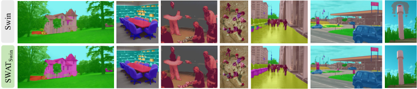
Figure A.1: Segmentation masks generated with UperNet Xiao et al. (2018) with Swin-Ti Liu et al. (2021) (our setting) and SWAT${}_{\text{Swin}}$-Ti as backbones. SWAT shows better segmentation results in comparison. Note the fine structures better captured by SWAT, thanks to preserved spatial information within tokens. Best viewed in color and zoomed-in.

Model	$\;\;\alpha\;\;$	Kernel	Top-1	FLOPs
Mixer (Tolstikhin et al.)	-	-	68.3%	0.97G
	2	$(5\times 5)$	70.9%	0.98G
	4	$(5\times 5)$	71.1%	0.99G
SWAT${}_{\text{Mixer}}$	8	$(5\times 5)$	72.3%	0.99G
	8	$(3\times 3)$	69.8%	0.96G
	8	$(7\times 7)$	71.2%	1.02G

Table A.1: Ablations on (1) the granularity of preserved structure, and (2) the level of structure-awareness in mixing, with SWAT${}_{\text{Mixer}}$-Ti models on ImageNet-1K. With structure hyperparameter $\alpha$, we preserve an $\alpha\times\alpha$ structure within tokens. Increasing granularity (i.e., preserving finer details) shows consistent performance gains. Kernel size in Mixing decides how-well we utilize the structure (i.e., structure-awareness). In Token Mixing, we fix Conv kernel to be $(3\times 3)$ due to spatial size constraints. In Channel mixing, we consider kernel sizes of {3,5,7}. Conv kernels of $(5\times 5)$ shows the best performance at a similar complexity as the baseline.

Receptive field when utilizing structure:

We always consider $3\times 3$ Conv kernels for token mixing (since the input spatial dimension $h\times w$ within tokens is only $8\times 8$) in these settings. However, we can consider kernel sizes of $\{3,5,7\}$ in channel mixing (since the input spatial dimension $H/p\times W/p$ among tokens is $14\times 14$). Higher kernel size means we exploit more structure in Mixing, but also, it increases both parameters and computations as well. In Table A.1, we see that $5\times 5$ kernels shows the best performance at a similar complexity as in the baseline Mixer Tolstikhin et al. (2021).

SWAT regular patch-size vs. Baseline small patch-size:

If we simply consider smaller patch-sizes to preserve fine-grained information instead of a SWAT-like implementation, it will either blow-up the computations or lack the model capacity. For instance, a transformer block has $12C^{2}$ parameters, whereas the FLOP count scales with $(12NC^{2}+2N^{2}C)$. Here, $C$ is number of channels and $N$ is number of tokens. If we directly reduce the patch-size, it will give more tokens, increasing the computations quadratically. We can contain this by reducing the channel size, but it will also reduce the number of parameters, sacrificing the model capacity. In contrast, SWAT retains the fine-grained information similar to a model with smaller patch-size, but at the same footprint as a model with original patch-size.

Segmentation masks:

Fig. A.1 shows qualitative results of SWAT${}_{\text{Swin}}$ on semantic segmentation, compared to its baseline. Our model achieves better segmentation masks with a focus on fine-grained details and coherent structure.

Exceptions to the default training schedule and input resolution:

In general, we compare against models trained for 300 epochs at $224\times 224$ resolution. However, some baselines in Table 2 have different settings, namely, ResNeXt: 90 epochs, RegNetY: 100 epochs, ResMLP: 400 epochs, MobileFormer: 450 epochs and EfficientNet: $380\times 380$ resolution.

6.2 Throughput of SWAT models

Model	Top-1	Params.	FLOPs	Throughput
	(%)	(M)	(G)	(im/s)
DeiT - Ti (Touvron et al.)	72.2	5.7	1.3	2391
SWAT${}_{\text{DeiT}}$ - Ti	75.7	5.8	1.4	1330
DeiT - S (Touvron et al.)	79.8	22.1	4.6	924
SWAT${}_{\text{DeiT}}$ - S	80.5	22.3	4.9	645
DeiT/32 - B (Touvron et al.)	75.5	88.2	4.3	1275
SWAT${}_{\text{DeiT}}$/32 - B	76.2	86.3	4.5	923
Mixer - Ti (Tolstikhin et al.)	68.3	5.1	1.0	3701
SWAT${}_{\text{Mixer}}$ - Ti	72.3	5.1	1.0	2759
Mixer - S (Tolstikhin et al.)	75.7	18.5	3.8	1235
SWAT${}_{\text{Mixer}}$ - S	77.9	18.6	3.8	1022
Swin - Ti (Liu et al.)	81.3	28.3	4.5	703
SWAT${}_{\text{Swin}}$ - Ti	81.7	27.1	4.7	402
ResMLP (Touvron et al.)	76.6	15.4	3.0	1562
SWAT${}_{\text{ResMLP}}$	77.8	15.6	3.1	1136

Table A.2: Throughput analysis of different SWAT models: We report performance and complexity (params., FLOPs and Throughput). System-agnostic metrics (params. and FLOPs) show consistent changes. However, throughput (on a single V100) show interesting variations: (1) smaller changes in larger models, and (2) changes in Transformer models are relatively higher than in Mixer models.

Model	Structure-aware			Top-1	Params.	FLOPs	Thrput.
	Tk.	TM	CM	(%)	(M)	(G)	(im/s)
DeiT				73.3	5.72	1.25	2391
			✓	74.6	5.96	1.30	1911
		✓		73.7	5.72	1.30	1778
	✓			73.0	5.58	1.30	2008
	✓	✓		74.5	5.59	1.35	1551
SWAT${}_{\text{DeiT}}$	✓	✓	✓	75.7	5.83	1.40	1330
Mixer				68.3	5.07	0.97	3701
			✓	70.8	5.28	1.01	3053
		✓		68.9	5.08	0.97	3534
	✓			67.9	4.88	0.94	3452
	✓	✓		70.2	4.88	0.95	3215
SWAT${}_{\text{Mixer}}$	✓	✓	✓	72.3	5.10	0.99	2759

Table A.3: Throughput analysis of SWAT ablations: We report performance and complexity (params., FLOPs and Throughput). Each SWAT model shows small changes in system-agnostic metrics compared to the corresponding baseline. However, throughput changes are inconsistent in general. Our tokenization costs $-16\%$ in DeiT Touvron et al. (2021b), but only $-7\%$ in Mixer Tolstikhin et al. (2021). Our token mixing costs $-25\%$ throughput in DeiT, but only $-5\%$ in Mixer. In contrast, channel mixing costs are comparable, with $-20\%$ and $-17\%$, in DeiT and Mixer respectively.

Mixer Block configuration	Struct.	Throughput (im/s)
	tokens	V100	A100
$2\times$ Linear		3701	9127
$2\times$ 1D Conv (P)		3441	6921
$2\times$ 2D Conv (P)		3716	7421
$2\times$ 1D Conv (P) + $1\times$ Linear		2496	5480
$2\times$ 2D Conv (P) + $1\times$ Linear		2440	5290
$2\times$ 2D Conv (P) + $1\times$ 2D Conv (D)		2927	5538
$2\times$ 2D Conv (P) + $1\times$ 2D Conv (D)	✓	2759	5112

Table A.4: Throughput analysis of different SWAT${}_{\text{Mixer}}$ block configurations: We report performance and complexity (params., FLOPs and Throughput— measured on a single V100/A100). Here, (P) represents Pointwise and (D), Depthwise Conv. Throughputs depend on the hardware, and different cuda implementations. On A100s, Linear layers are significantly faster than Conv (P). Even though Linear, 1D Conv (P) and 2D Conv (P) perform the same operation, they have different throughputs. Additional Linear layers incur higher cost compared to 2D Conv (D) on V100, which is not the case on A100.

In this paper, we consider FLOPs as the main complexity metric, since it is system-agnostic. Here, we report throughput numbers using PyTorch 1.7.1 on a single V100 GPU. These may change depending on the actual hardware and underlying cuda optimizations.

With model scale:

When we consider larger SWAT models, the change of throughput due to Structure-aware Tokenization and Mixing becomes small (see Table A.2). In DeiT Touvron et al. (2021b), we see a $-44\%$ change in Tiny, $-30\%$ in Small and $-28\%$ in Base/32 models. We see a $-25\%$ change in Tiny and $-17\%$ in Small models in Mixer Tolstikhin et al. (2021). However, none of the SWAT models have significant change in system-agnostic measures such as parameters or FLOPs.

In Transformers vs. Mixers:

The change in throughput with Transformer models such as DeiT-Ti ($-44\%$) Touvron et al. (2021b) or Swin-Ti Liu et al. (2021) ($-43\%$) is higher compared to Mixer models such as Mixer-Ti Tolstikhin et al. (2021) ($-25\%$) or ResMLP-S12 Touvron et al. (2021a) ($-27\%$) (see Table A.2 and Table A.3). The difference between models is in Token Mixing. In Transformers, SWAT includes additional $2\times$ parallel 2D Conv blocks, whereas in Mixers, $1\times$ cascaded 2D Depthwise Conv block. 2D Conv blocks in Transformers see small feature depths (eg: depth$=3$ in Tiny) and run in parallel to Linear layers, which makes it hard to justify the extra throughput cost compared to cascaded 2D Depthwise Conv in Mixers. This shows inconsistency in cuda optimizations for different operators.

Using Linear vs. Conv:

Same operation as a Linear layer can be performed using 1D or 2D Pointwise Conv. However, in terms of throughput, Pointwise Conv layers show differences compared to Linear layers both on V100s ($-7\%$ w/ 1D and $0\%$ w/ 2D) and on A100s ($-24\%$ w/ 1D and $-19\%$ w/ 2D). See Table A.4. This shows differences in cuda optimizations, even for essentially-the-same operation.

On V100 vs. A100:

We see striking differences in throughput variations on V100 compared to A100 (see Table A.4). On A100s, implementation of Linear layers seems to be much faster compared to Pointwise Conv. This difference in throughput directly propagates to SWAT models.

Looking at the above inconsistencies in measuring complexity as throughput, we consider system-agnostic measures such as parameters or FLOPs to be more reliable and reproducible metrics to be evaluated in this paper.

References

- Arnab et al. [2021] Anurag Arnab, Mostafa Dehghani, Georg Heigold, Chen Sun, Mario Lučić, and Cordelia Schmid. ViViT: A Video Vision Transformer. In ICCV, October 2021.
- Bello [2020] Irwan Bello. LambdaNetworks: Modeling long-range Interactions without Attention. In ICLR, 2020.
- Cao et al. [2021] Jiezhang Cao, Yawei Li, Kai Zhang, and Luc Van Gool. Video Super-Resolution Transformer. arXiv:2106.06847, 2021.
- Carion et al. [2020] Nicolas Carion, Francisco Massa, Gabriel Synnaeve, Nicolas Usunier, Alexander Kirillov, and Sergey Zagoruyko. End-to-End Object Detection with Transformers. In ECCV. Springer, 2020.
- Caron et al. [2021] Mathilde Caron, Hugo Touvron, Ishan Misra, Hervé Jégou, Julien Mairal, Piotr Bojanowski, and Armand Joulin. Emerging Properties in Self-Supervised Vision Transformers. In ICCV, October 2021.
- Chen et al. [2018] Liang-Chieh Chen, Yukun Zhu, George Papandreou, Florian Schroff, and Hartwig Adam. Encoder-Decoder with Atrous Separable Convolution for Semantic Image Segmentation. In ECCV, 2018.
- Chen et al. [2021a] Lili Chen, Kevin Lu, Aravind Rajeswaran, Kimin Lee, Aditya Grover, Michael Laskin, Pieter Abbeel, Aravind Srinivas, and Igor Mordatch. Decision Transformer: Reinforcement Learning via Sequence Modeling. URL Workshop in ICML, 2021.
- Chen et al. [2021b] Shoufa Chen, Enze Xie, Chongjian Ge, Ding Liang, and Ping Luo. CycleMLP: A MLP-like Architecture for Dense Prediction. arXiv:2107.10224, 2021.
- Chen et al. [2022] Yinpeng Chen, Xiyang Dai, Dongdong Chen, Mengchen Liu, Xiaoyi Dong, Lu Yuan, and Zicheng Liu. Mobile-former: Bridging mobilenet and transformer. In CVPR, 2022.
- Chu et al. [2021] Xiangxiang Chu, Zhi Tian, Yuqing Wang, Bo Zhang, Haibing Ren, Xiaolin Wei, Huaxia Xia, and Chunhua Shen. Twins: Revisiting the design of spatial attention in vision transformers. NeurIPS, 34, 2021.
- Dai et al. [2021] Zhigang Dai, Bolun Cai, Yugeng Lin, and Junying Chen. UP-DETR: Unsupervised Pre-training for Object Detection with Transformers. In CVPR, 2021.
- Dai et al. [2022] Rui Dai, Srijan Das, Kumara Kahatapitiya, Michael S Ryoo, and Francois Bremond. MS-TCT: Multi-Scale Temporal ConvTransformer for Action Detection. In CVPR, 2022.
- Dauphin et al. [2017] Yann N Dauphin, Angela Fan, Michael Auli, and David Grangier. Language Modeling with Gated Convolutional Networks. In ICML. PMLR, 2017.
- Deng et al. [2009] Jia Deng, Wei Dong, Richard Socher, Li-Jia Li, Kai Li, and Li Fei-Fei. Imagenet: A large-scale hierarchical image database. In CVPR. IEEE, 2009.
- Devlin et al. [2019] Jacob Devlin, Ming-Wei Chang, Kenton Lee, and Kristina Toutanova. BERT: Pre-training of deep bidirectional transformers for language understanding. In NAACL-HLT. Association for Computational Linguistics, June 2019.
- Dosovitskiy et al. [2021] Alexey Dosovitskiy, Lucas Beyer, Alexander Kolesnikov, Dirk Weissenborn, Xiaohua Zhai, Thomas Unterthiner, Mostafa Dehghani, Matthias Minderer, Georg Heigold, Sylvain Gelly, et al. An Image is Worth 16x16 Words: Transformers for Image Recognition at Scale. ICLR, 2021.
- Duke et al. [2021] Brendan Duke, Abdalla Ahmed, Christian Wolf, Parham Aarabi, and Graham W Taylor. SSTVOS: Sparse Spatiotemporal Transformers for Video Object Segmentation. In CVPR, 2021.
- d’Ascoli et al. [2021] Stéphane d’Ascoli, Hugo Touvron, Matthew L Leavitt, Ari S Morcos, Giulio Biroli, and Levent Sagun. ConViT: Improving Vision Transformers with Soft Convolutional Inductive Biases. In ICML. PMLR, 2021.
- Esser et al. [2021] Patrick Esser, Robin Rombach, and Bjorn Ommer. Taming Transformers for High-Resolution Image Synthesis. In CVPR, 2021.
- Fan et al. [2021] Haoqi Fan, Bo Xiong, Karttikeya Mangalam, Yanghao Li, Zhicheng Yan, Jitendra Malik, and Christoph Feichtenhofer. Multiscale Vision Transformers. In ICCV, October 2021.
- Fu et al. [2019a] Jun Fu, Jing Liu, Haijie Tian, Yong Li, Yongjun Bao, Zhiwei Fang, and Hanqing Lu. Dual Attention Network for Scene Segmentation. In CVPR, 2019.
- Fu et al. [2019b] Jun Fu, Jing Liu, Yuhang Wang, Yong Li, Yongjun Bao, Jinhui Tang, and Hanqing Lu. Adaptive Context Network for Scene Parsing. In ICCV, 2019.
- Graham et al. [2021] Benjamin Graham, Alaaeldin El-Nouby, Hugo Touvron, Pierre Stock, Armand Joulin, Hervé Jégou, and Matthijs Douze. LeViT: A Vision Transformer in ConvNet’s Clothing for Faster Inference. In ICCV, October 2021.
- Guo et al. [2021] Meng-Hao Guo, Jun-Xiong Cai, Zheng-Ning Liu, Tai-Jiang Mu, Ralph R Martin, and Shi-Min Hu. PCT: Point Cloud Transformer. Computational Visual Media, 7(2), 2021.
- Guo et al. [2022] Meng-Hao Guo, Cheng-Ze Lu, Zheng-Ning Liu, Ming-Ming Cheng, and Shi-Min Hu. Visual Attention Network. arXiv:2202.09741, 2022.
- Han et al. [2021] Kai Han, An Xiao, Enhua Wu, Jianyuan Guo, Chunjing Xu, and Yunhe Wang. Transformer in Transformer. In NeurIPS, 2021.
- He et al. [2016] Kaiming He, Xiangyu Zhang, Shaoqing Ren, and Jian Sun. Deep Residual Learning for Image Recognition. In CVPR, 2016.
- Heo et al. [2021] Byeongho Heo, Sangdoo Yun, Dongyoon Han, Sanghyuk Chun, Junsuk Choe, and Seong Joon Oh. Rethinking Spatial Dimensions of Vision Transformers. In ICCV, 2021.
- LeCun et al. [2015] Yann LeCun, Yoshua Bengio, and Geoffrey Hinton. Deep Learning. Nature, 521(7553), 2015.
- Liu et al. [2021] Ze Liu, Yutong Lin, Yue Cao, Han Hu, Yixuan Wei, Zheng Zhang, Stephen Lin, and Baining Guo. Swin Transformer: Hierarchical Vision Transformer Using Shifted Windows. In ICCV, October 2021.
- Liu et al. [2022] Zhuang Liu, Hanzi Mao, Chao-Yuan Wu, Christoph Feichtenhofer, Trevor Darrell, and Saining Xie. A ConvNet for the 2020s. In CVPR, 2022.
- Nagrani et al. [2021] Arsha Nagrani, Shan Yang, Anurag Arnab, Aren Jansen, Cordelia Schmid, and Chen Sun. Attention Bottlenecks for Multimodal Fusion. NeurIPS, 34, 2021.
- Naseer et al. [2021] Muzammal Naseer, Kanchana Ranasinghe, Salman Khan, Munawar Hayat, Fahad Shahbaz Khan, and Ming-Hsuan Yang. Intriguing Properties of Vision Transformers. In NeurIPS, 2021.
- OpenMMLab [2020] OpenMMLab. MMSegmentation: OpenMMLab Semantic Segmentation Toolbox and Benchmark. https://github.com/open-mmlab/mmsegmentation, 2020. Accessed: 2023-01-18.
- Peng et al. [2021] Zhiliang Peng, Wei Huang, Shanzhi Gu, Lingxi Xie, Yaowei Wang, Jianbin Jiao, and Qixiang Ye. Conformer: Local Features Coupling Global Representations for Visual Recognition. In ICCV, October 2021.
- Radosavovic et al. [2020] Ilija Radosavovic, Raj Prateek Kosaraju, Ross Girshick, Kaiming He, and Piotr Dollár. Designing network design spaces. In CVPR, 2020.
- Ranasinghe et al. [2022] Kanchana Ranasinghe, Muzammal Naseer, Salman Khan, Fahad Shahbaz Khan, and Michael S Ryoo. Self-supervised Video Transformer. In CVPR, 2022.
- Ranftl et al. [2021] René Ranftl, Alexey Bochkovskiy, and Vladlen Koltun. Vision Transformers for Dense Prediction. In ICCV, 2021.
- Ryoo et al. [2021] Michael S Ryoo, AJ Piergiovanni, Anurag Arnab, Mostafa Dehghani, and Anelia Angelova. TokenLearner: Adaptive Space-Time Tokenization for Videos. In NeurIPS, 2021.
- Shang et al. [2022] Jinghuan Shang, Kumara Kahatapitiya, Xiang Li, and Michael S Ryoo. StARformer: Transformer with State-Action-Reward Representations. In ECCV, 2022.
- Tan and Le [2019] Mingxing Tan and Quoc Le. EfficientNet: Rethinking Model Scaling for Convolutional Neural Networks. In ICML. PMLR, 2019.
- Tang et al. [2021] Chuanxin Tang, Yucheng Zhao, Guangting Wang, Chong Luo, Wenxuan Xie, and Wenjun Zeng. Sparse MLP for Image Recognition: Is Self-Attention Really Necessary? arXiv:2109.05422, 2021.
- Tolstikhin et al. [2021] Ilya Tolstikhin, Neil Houlsby, Alexander Kolesnikov, Lucas Beyer, Xiaohua Zhai, Thomas Unterthiner, Jessica Yung, Andreas Peter Steiner, Daniel Keysers, Jakob Uszkoreit, et al. MLP-Mixer: An All-MLP Architecture for Vision. In NeurIPS, 2021.
- Touvron et al. [2021a] Hugo Touvron, Piotr Bojanowski, Mathilde Caron, Matthieu Cord, Alaaeldin El-Nouby, Edouard Grave, Gautier Izacard, Armand Joulin, Gabriel Synnaeve, Jakob Verbeek, et al. ResMLP: Feedforward networks for image classification with data-efficient training. arXiv:2105.03404, 2021.
- Touvron et al. [2021b] Hugo Touvron, Matthieu Cord, Matthijs Douze, Francisco Massa, Alexandre Sablayrolles, and Hervé Jégou. Training data-efficient image transformers & distillation through attention. In ICML. PMLR, 2021.
- Trockman and Kolter [2022] Asher Trockman and J Zico Kolter. Patches are all you need? arXiv:2201.09792, 2022.
- Vaswani et al. [2017] Ashish Vaswani, Noam Shazeer, Niki Parmar, Jakob Uszkoreit, Llion Jones, Aidan N Gomez, Łukasz Kaiser, and Illia Polosukhin. Attention Is All You Need. In NeurIPS, 2017.
- Wang et al. [2018] Xiaolong Wang, Ross Girshick, Abhinav Gupta, and Kaiming He. Non-local Neural Networks. In CVPR, 2018.
- Wang et al. [2021] Wenhai Wang, Enze Xie, Xiang Li, Deng-Ping Fan, Kaitao Song, Ding Liang, Tong Lu, Ping Luo, and Ling Shao. Pyramid Vision Transformer: A Versatile Backbone for Dense Prediction Without Convolutions. In ICCV, October 2021.
- Wightman [2019] Ross Wightman. Pytorch Image Models. https://github.com/rwightman/pytorch-image-models, 2019. Accessed: 2023-01-18.
- Wu et al. [2021] Haiping Wu, Bin Xiao, Noel Codella, Mengchen Liu, Xiyang Dai, Lu Yuan, and Lei Zhang. CvT: Introducing Convolutions to Vision Transformers. In ICCV, October 2021.
- Xiao et al. [2018] Tete Xiao, Yingcheng Liu, Bolei Zhou, Yuning Jiang, and Jian Sun. Unified Perceptual Parsing for Scene Understanding. In ECCV, 2018.
- Xiao et al. [2021] Tete Xiao, Piotr Dollar, Mannat Singh, Eric Mintun, Trevor Darrell, and Ross Girshick. Early Convolutions Help Transformers See Better. In NeurIPS, 2021.
- Xie et al. [2017] Saining Xie, Ross Girshick, Piotr Dollár, Zhuowen Tu, and Kaiming He. Aggregated residual transformations for deep neural networks. In CVPR, 2017.
- Xie et al. [2021] Enze Xie, Wenhai Wang, Zhiding Yu, Anima Anandkumar, Jose M Alvarez, and Ping Luo. SegFormer: Simple and Efficient Design for Semantic Segmentation with Transformers. In NeurIPS, 2021.
- Yang et al. [2021a] Guanglei Yang, Hao Tang, Mingli Ding, Nicu Sebe, and Elisa Ricci. Transformer-Based Attention Networks for Continuous Pixel-Wise Prediction. In ICCV, 2021.
- Yang et al. [2021b] Jianwei Yang, Chunyuan Li, Pengchuan Zhang, Xiyang Dai, Bin Xiao, Lu Yuan, and Jianfeng Gao. Focal Self-attention for Local-Global Interactions in Vision Transformers. In NeurIPS, 2021.
- Yin et al. [2020] Minghao Yin, Zhuliang Yao, Yue Cao, Xiu Li, Zheng Zhang, Stephen Lin, and Han Hu. Disentangled Non-Local Neural Networks. In ECCV. Springer, 2020.
- Yu et al. [2022] Weihao Yu, Mi Luo, Pan Zhou, Chenyang Si, Yichen Zhou, Xinchao Wang, Jiashi Feng, and Shuicheng Yan. Metaformer is actually what you need for vision. In CVPR, 2022.
- Yuan et al. [2021a] Kun Yuan, Shaopeng Guo, Ziwei Liu, Aojun Zhou, Fengwei Yu, and Wei Wu. Incorporating Convolution Designs Into Visual Transformers. In ICCV, October 2021.
- Yuan et al. [2021b] Li Yuan, Yunpeng Chen, Tao Wang, Weihao Yu, Yujun Shi, Zi-Hang Jiang, Francis E.H. Tay, Jiashi Feng, and Shuicheng Yan. Tokens-to-Token ViT: Training Vision Transformers From Scratch on ImageNet. In ICCV, October 2021.
- Yue et al. [2021] Xiaoyu Yue, Shuyang Sun, Zhanghui Kuang, Meng Wei, Philip H.S. Torr, Wayne Zhang, and Dahua Lin. Vision Transformer With Progressive Sampling. In ICCV, October 2021.
- Zhai et al. [2021] Shuangfei Zhai, Walter Talbott, Nitish Srivastava, Chen Huang, Hanlin Goh, Ruixiang Zhang, and Josh Susskind. An Attention Free Transformer. arXiv:2105.14103, 2021.
- Zhang et al. [2021] Zizhao Zhang, Han Zhang, Long Zhao, Ting Chen, and Tomas Pfister. Aggregating Nested Transformers. arXiv:2105.12723, 2021.
- Zhao et al. [2020] Hengshuang Zhao, Jiaya Jia, and Vladlen Koltun. Exploring Self-attention for Image Recognition. In CVPR, 2020.
- Zhao et al. [2021] Hengshuang Zhao, Li Jiang, Jiaya Jia, Philip HS Torr, and Vladlen Koltun. Point Transformer. In ICCV, 2021.
- Zhou et al. [2019] Bolei Zhou, Hang Zhao, Xavier Puig, Tete Xiao, Sanja Fidler, Adela Barriuso, and Antonio Torralba. Semantic Understanding of Scenes Through the ADE20K Dataset. IJCV, 127(3), 2019.
- Zhu et al. [2020] Xizhou Zhu, Weijie Su, Lewei Lu, Bin Li, Xiaogang Wang, and Jifeng Dai. Deformable DETR: Deformable Transformers for End-to-End Object Detection. In ICLR, 2020.