A Reinforcement Learning Approach for the Continuous Electricity Market of Germany: Trading from the Perspective of a Wind Park Operator

Abstract

With the rising extension of renewable energies, the intraday electricity markets have recorded a growing popularity amongst traders as well as electric utilities to cope with the induced volatility of the energy supply. Through their short trading horizon and continuous nature, the intraday markets offer the ability to adjust trading decisions from the day-ahead market or reduce trading risk in a short-term notice. Producers of renewable energies utilize the intraday market to lower their forecast risk, by modifying their provided capacities based on current forecasts. However, the market dynamics are complex due to the fact that the power grids have to remain stable and electricity is only partly storable. Consequently, robust and intelligent trading strategies are required that are capable to operate in the intraday market. In this work, we propose a novel autonomous trading approach based on Deep Reinforcement Learning (DRL) algorithms as a possible solution. For this purpose, we model the intraday trade as a Markov Decision Process (MDP) and employ the Proximal Policy Optimization (PPO) algorithm as our DRL approach. A simulation framework is introduced that enables the trading of the continuous intraday price in a resolution of one minute steps. We test our framework in a case study from the perspective of a wind park operator. We include next to general trade information both price and wind forecasts. On a test scenario of German intraday trading results from 2018, we are able to outperform multiple baselines with at least 45.24% improvement, showing the advantage of the DRL algorithm. However, we also discuss limitations and enhancements of the DRL agent, in order to increase the performance in future works.

Keywords Deep Reinforcement Learning  $\cdot$ German Intraday Electricity Trading  $\cdot$ Deep Neural Networks  $\cdot$ Markov Decision Process  $\cdot$ Proximal Policy Optimization  $\cdot$ Electricity Price Forecast

1 Introduction

Acronyms

A3C

Asynchronous Advantage Actor-Critic

DA

Day-Ahead

DRL

Deep Reinforcement Learning

ID

Intraday

LOB

Limit Order Book

LSTM

Long Short-Term Memory

MDP

Markov Decision Process

ML

Machine Learning

PBT

Population Based Training

PPO

Proximal Policy Optimization

p.t.d

prior to delivery

RE

Renweable Energie

RL

Reinforcement Learning

RNN

Recurrent Neural Network

SGD

Stochastic gradient decent

1.1 Overview

In past decades, the day-ahead electricity markets were the major trading location to auction electricity capacities between market participants. However, with the European Green Deal [1] and the rising proportion of Renweable Energie (RE) production [2], there is a need for a higher flexibility in the electricity trade. Both electricity providers and prosumers require short-term solutions to respond to market changes and reduce their overall trading risk [3, 4]. One possible solution is the Intraday (ID) market that enable trading with less than one day prior to the delivery. Here, especially RE producers can anticipate changes in their production forecast and modify their orders from the day-ahead market to ensure an accurate delivery. Consequently, the ID electricity markets have an increasing popularity amongst traders, resulting in record trading volumes across all European ID electricity spot markets in 2020[5]. Similarly, in the research community there has been a rising interest in the analysis of the ID trade. The ID trade was examined from various perspectives, given that both the expansion of RE as well as the design of the ID markets differ across nations.In many cases the ID markets have been analyzed from a structural point of view, e.g., for the identification of influencing factors [6]. However, actual trading strategies have not been part of many analysis, considering that ID trading is not comparable to other commodity markets. With its short-term perspective, the strong influence of the RE, the volatility and the stochastic nature of the ID market, traditional trading methods are often not applicable. Consequently, alternative methods have to be investigated that can cope with these difficulties.
In our work, we want to contribute to this open question, by proposing an autonomous trading agent based on Deep Reinforcement Learning (DRL). While the autonomous approaches is primarily designed to compensate forecast errors on the ID market, it also contribute to more system stability. Especially in combination with flexible energy providers, autonomous agents could be deployed in the long run to counteract against potential surpluses and thus reduce the risk of shortfalls in the electricity distribution. In order to ensure a realistic setting, the autonomous agent is deployed from the perspective of an electricity provider, specifically a wind park operator. Given that wind forecasts always contain some uncertainty, wind park operators have to incorporate this uncertainty in their production plan. Hence, they can not exactly determine their produced volume a priori. The autonomous agent has to adjust the traded volumes on the ID markets based on recent changes in the forecasts.

1.2 Related Work

In terms of the research community, various topics regarding the ID market have been publicized. Many of them can be categorized either in the field of structural analysis, price forecasting or in the field of ID trading. In the first category, papers have been published that examined and analyzed different influencing factors on the ID markets [3, 7, 6, 8, 9]. Naturally, most of the papers reviewed the variability of the ID trade and were sometimes combined with an analysis of the RE or their forecasting errors [6]. However, these analysis focused in most cases on a longer time horizon, thus are not always suited for a direct application. In contrast, the second topic of electricity price forecasting considers the short-term relationship between prices and their influencing factors, as seen in [10, 11, 12, 13, 14]. However, next to differences in the markets and the forecast models, the research often differed in the frequency of the forecast target. As example, [10] predicted the ID3 index of the German ID market, while [11, 14] predicted the price movement of individual products. As a consequence, different influencing factors were of importance for the different researchers.
Lastly, the third research subject is the trading of electricity and its automation on the ID market, where for example Machine Learning (ML) approaches were frequently published by different researchers, e.g., [15, 16]. In recent years, a new ML approach was proposed that is especially suited to cope with the volatile price progression and the stochastic nature of the ID market. This respective approach is DRL, which can model complex relations and at the same time does not necessarily require expert knowledge of the trade relations. Accordingly, there have been first publications for both the Day-Ahead (DA) and ID market that addressed the challenges of the electricity trade in combination with DRL. In terms of the DA, the researchers utilized the DRL benefits to automatize and optimize the bidding process, sometimes in combination with the ID market. These bidding processes could be from the perspective of one [17] or multiple [18] producers, a load serving entity [19] or a electric storage unit [20]. For the ID market, especially the papers of [21, 22, 23] are noteworthy, which proposed trading strategies for the German continuous ID market. All three papers based their strategy on a Markov Decision Process (MDP), however differed in their algorithmic implementation and their research objective. In the paper of [21], Reinforcement Learning (RL) was used to implement a threshold policy for accepting price bids in the ID market. To determine the optimal policy, they defined an one-stage MDP and used the REINFORCE algorithm to solve the problem. A different use-case was proposed by [22, 23], who both analyzed the trading under the consideration that they need to optimize the usage of an energy or pump storage unit. Through the assumption that the electricity can be stored, they were able to formulate the trading in a multi-stage MDP. In terms of [22], a Deep-Q network was implemented as DRL method, while [23] again applied the REINFORCE algorithm. Even though [23] showed the most advanced modelling of the ID trade, they still needed to impose some simplifications to reduce the dimensionality of the optimization problem. Accordingly, they incorporated price thresholds to limit the number of available orders and traded in 24 time steps for each day. By reducing the number of observations per episode, [23] were able to implement their DRL approach with satisfying results. However, under consideration that the ID trade is indeed traded in milliseconds, there is still a need to improve the DRL to make it applicable for the ID trade. In our work, we address this problem and offer the next step in the development of an autonomous trading agent.

1.3 Research Contribution

As outlined in the related work section, there are still unanswered questions concerning the ID electricity trade. Especially, the continuous nature and the resulting shortest-term perspective of the electricity trade has not been part of an investigation. However, given the increasing number of trades and the induced uncertainty of the RE, there is a practical need to analyze the capabilities of autonomous trading. Therefore, the contributions of this paper can be outlined as follows:

1. We model the ID market as a (first-order) MDP and propose DRL approach to simulate the continuous ID trade.

2. We develop a DRL environment based on the OpenAI library [24] with a shortest-term perspective in one minute resolution. To the best of our knowledge, this has not been part of any analysis and offers new insights to the electricity trade.

3. We validate our proposed DRL problem from the perspective of an electricity producer that trades the capacities of his wind turbine on the German ID market.

4. Within our case study, we are able to show that the proposed DRL agent is able to trade volatile wind volumes in the ID simulation.

5. The DRL agent outperforms the best baseline agent with 45.24% more net profit in our case study.

With the outlined research contribution, the remaining paper is structured as follows. In Section 2, the methodology of the underlying DRL is presented. In Section 3 we transfer the framework to the scenario of the ID spot market. Thereafter, we elaborate our case study in Section 4 and present and discuss the results in Section 5. Lastly, in Section 6 we give an overall conclusion.

2 Methodology

2.1 Reinforcement Learning as Markov Decision Process

From the area of machine learning methods, the Reinforcement Learning (RL) is an approach first introduced by [25]. It is based on the concept that a model can solve complex problems without outlining the exact relations but instead by learning the correct behavior through incentives in the training process.

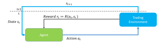
Figure 1: Visualization of the DRL-Framework with environment and agent. Based on the state $s_{t}$ of the environment, the agent computes the action $a_{t}$. The action is returned, the reward $r_{t}$ calculated and saved for the optimization. Thereafter, the environment transitions to the new state $s_{t+1}$.

In the RL approach, an agent is trained in an environment $\mathbb{S}$ that incorporates the structure of the real-life problem. The environment iterates over consecutive steps, as seen in Figure 1, until an episode is complete. For each step of the episode, the agent can take different actions $a\in\mathbb{A}$, with $\mathbb{A}$ denoting the space of possible actions. The purpose of the environment is the communication with the RL agent, by supplying the information on its current state $s_{t}\in\mathbb{S}$ at time $t$ and returning a feedback on the actions $a_{t}$ in form of a reward $r\in\ \mathbb{R}$ with $r_{t}:=R(a_{t},s_{t})$, based on the reward function $R:\mathbb{A}\times\mathbb{S}\to\mathbb{R}$. Within the episode of length $T$, the target of the RL algorithm is to maximize the cumulative reward $\tilde{R}_{cum}:=\sum_{t=1}^{T}r_{t}$. In each step, the agent consequently chooses the action, which promises the best possible payout, considering all future actions. To correctly define the impact of each action, all the future reward arising from the action has to be considered. For this purpose, the RL problem is assumed to be a MDP, i.e., a (time-discrete) stochastic process $\{M\}_{t\in T}$ on a probability space $(\Omega,\mathcal{A},\mathbb{P})$ with $t$ denoting the set of time steps $\{0,1,\ldots,T\}$, fulfilling the first-order Markov property for all $t\in T$, and all state-action pairs $(a_{t},s_{t})\in\mathbb{A}\times\mathbb{S}$:

$$\mathbb{P}(s_{t+1}|a_{t},s_{t})=\mathbb{P}(s_{t+1}|a_{t},s_{t},\ldots,a_{0},s_{0}).$$ (1)

Here, $\mathbb{P}$ is the transition probability to reach state $s_{t+1}$ from state $s_{t}$ taking action $a_{t}$. In a first-order MDP, not all past information about the process are required to asses the probability, but instead the current state $s_{t}$ and the action $a_{t}$ are sufficient enough. The consequence of assuming a MDP for the RL approach is that the RL algorithms need to approximate the underlying transition probability $\mathbb{P}$ and selects actions, which result in states leading to a higher reward. In RL terms, policies $\pi_{\theta}$ are probability distributions in each state $s_{t}$ over all the possible actions $a_{t}\in\mathbb{A}$. Each probability $\pi(\cdot|s_{t})$ denotes the likelihood of the respective action to yield the maximum reward over the whole episode. Note that next to the current state $s_{t}$, the policies depend on an underlying parameter $\theta$. In the Deep Reinforcement Learning (DRL) approach, first introduced by [26], these parameters are the weights of a deep neural network, representing the policy and thereby the action selection behavior. Through optimizing the weights of the network, DRL algorithms aim to approximate the optimal policy $\pi^{*}:=\pi_{\theta^{*}}$ offering the best decision for each state $s_{t}\in\mathbb{S}$. With regard to each step, displayed in Figure 2, the network receives the current state $s_{t}$, as well as the previous reward $r_{t}$ for the policy optimization. The state information is forwarded to compute the policies $\pi_{\theta}(a^{i}_{t}|s_{t})$ of each available action $a^{i}_{t}$. Based on the best policy, an action $a^{*}_{t}$ is chosen, the reward $r_{t+1}=R(a^{*}_{t},s_{t})$ is computed and the next iteration step is started.

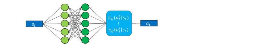
Figure 2: Exemplary neural network of the DRL approach. The hidden layers (green) pass the state $s_{t}$ and reward $r_{t}$ information to the policy layer (light blue). Thereafter, an action $a_{t}$ is chosen based on the policy.

2.2 Optimization Algorithm

There are various DRL algorithms available to update the policy $\pi(\theta)$ that mainly differ in their update strategy and the underlying relationship between policy $\pi(\theta)$ and parameters $\theta$. In our work, we chose the Proximal Policy Optimization (PPO) algorithm because it enables the usage of an continuous action space. It was firstly introduced in [28] and is an enhancement of the Asynchronous Advantage Actor-Critic (A3C) method [29]. In the PPO method, two neural networks are utilized to optimize the policy iteratively. The Actor model is deployed in the environment to generate observations by computing actions and obtaining rewards. The second model, i.e., the Critic, forecasts based on the observations the probable future rewards given a specific action. The difference between the forecasted and actual reward is then evaluated in an advantage function $\hat{A}_{t}(\theta)$. Actions leading to a positive advantage (so higher reward gained by Actor than forecasted by Critic) are reinforced while actions leading to negative advantage are discarded. This optimization problem is formulated as a loss function $L(\theta)$, with the objective to minimize the loss based on the expected return and the parameters $\theta$ of the DRL model:

$$L_{t}(\theta) =\hat{E}_{t}\left[\log\pi_{\theta}(a_{t}|s_{t})\hat{A}_{t}(\theta)\right].$$ (2)

To improve the weights of the actor, the loss function is optimized through a Stochastic gradient decent (SGD) method, which in case of the PPO is the Adam algorithm [30]. However, previous algorithms prior to the PPO had often instabilities in their learning process, due to large updates in their parameters $\theta$. As a consequence, [28] address this problem by introducing $\epsilon$-clipping in their loss function to limit the update of the optimization:

$$\begin{aligned} L_{t}^{CLIP}(\theta)\ =&\hat{E}_{t}\left[\min(\tau_{t}(\theta)\hat{A}_{t}(\theta),\Gamma_{clip})\right],\\[12.0pt] \text{with}\ \tau_{t}(\theta)=&\frac{\pi_{\theta}(a_{t}|s_{t})}{\pi_{\theta_{old}}(a_{t}|s_{t})},\\[12.0pt] \text{and}\ \Gamma_{clip}\ =&clip(\tau_{t}(\theta),1-\epsilon,1+\epsilon)\hat{A}_{t}(\theta).\end{aligned}$$ (3)

As one can see, the loss function is the estimated expectation of the minimum value of either $\tau_{t}(\theta)\hat{A}_{t}(\theta)$ or the clipped value $\Gamma_{clip}$. Very large positive updates in policy are clipped while negative updates are still considered valid. Thus, it is ensured that the updates are not running to a local maximum. Next to the optimization of the loss function, [28] further include other algorithmic advantages that enhance the optimization from a computational perspective. These are the parallel computation of multiple Actors, the introduction of mini-batches and the multiple runs of SGD on the same data. All of the advances increase learning speed and exploration of the environment as well as learning stability, thus making the PPO our preferred algorithm.

2.3 Hyperparameter Optimization

The PPO algorithm has various hyperparameters, which have considerable influence on the training performance. Therefore, we included a hyperparameter optimization in our analysis. Under consideration of the DRL characteristics, we decided to use the Population Based Training (PBT) hyperparameter search algorithm, based on the paper of [31]. The PBT is constructed with an evolutionary concept, where multiple variations of the algorithm are trained simultaneously and the most fitting candidate is selected. For this purpose, the hyperparameters of multiple DRL agents are randomly sampled. After a specific training period, the performance of the agents is evaluated and the better performing candidates can continue their training. For the underachieving agents, the hyperparameters are re-sampled and in addition the model states of the better candidates are copied. Therefore, no training progress is lost, while simultaneously different options are tested.

3 Research Design

3.1 General Research Setting

The trading environment is of huge importance for the overall success of the DRL algorithm and varies in the literature depending on the application of the agent. In our work, we construct research design from the perspective of a wind park operator, as stated in Section 1.1. As a consequence, the task of the trading agent is to react to the changes in the wind forecast of the producer and automatically conduct correction processes on the ID market. For this purpose, we combine our trading environment with external wind forecasts to train the agent. We evaluate our research on the German continuous ID electricity market, given that this market is frequently used in the literature, thus ensures comparability. Consequently, we shortly describe the structure of the continuous German ID market, derive restrictions and thereafter define our trading environment.

3.2 The German Continuous Intraday Electricity Market

The German ID short-term electricity trade is primarily conducted on the EPEX SPOT exchange, where different electricity products, e.g., quarterly and hourly products, are traded by the market participants in a continuous manner. In this research we solely focus on the hourly products, which we hereinafter just referred to as products. The ID trade is based on the M7 trading system, thus the trade is executed through an individual Limit Order Book (LOB) for each product, see [32]. In each LOB, open buy/sell orders are collected, sorted according to their highest/lowest price and matched if a new order with a lower sell/higher buy price is submitted. The matched orders are then recorded in the transaction data. For the hourly ID products, the trading interval starts at 3.00pm of the previous day and closes 5min prior to delivery (p.t.d), as seen in Figure 3. While the first hours of trade are open for both national and cross-border trade (trade on the XBID exchange), the trading is gradually restricted in conjunction with the distance to the delivery time. At one hour p.t.d only national trades are allowed, while in the last 30min until 5min p.t.d only trading in the control area is allowed. As a consequence, the trading behavior differs, depending on the delivery time and the respective market participants.

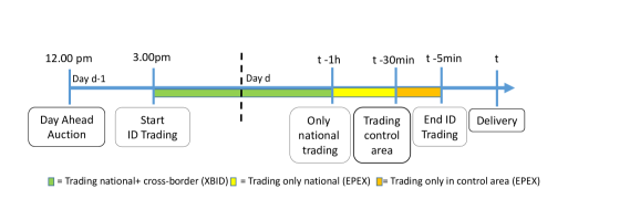
Figure 3: Overview over the trading stages of an ID product with delivery at day $d$ and time $t$. The trading starts at 3.00pm on the previous day $d-1$ and consist of national and cross-border trading. One hour p.t.d the cross-border trading stops, leaving national trading, and half an hour only trading in the control area is allowed.

3.3 Restriction for the Trading Environment

As a consequence of the ID trade structure, it was necessary to construct an environment for the DRL agent capturing both the essential information of the LOB, while simultaneously reducing their complexity. Thus, multiple restrictions were necessary to model an adequate simulation of the trades.

First, we decided to build our environment only with the transaction data of the ID market, which is in most cases close to the actual LOB. This has the advantage that the transaction data consists only of traded contracts, hence excludes the various cases of open orders, trade limitations, over the counter contracts and other redundant information. One consequence arising with this restriction is that we establish our agent as a price taker with no direct influence on the ID price. Under the assumption that the agent is only trading small amounts of energy, this seems reasonable. If one wants to trade a larger amount of electricity, multiple orders from the LOB have to be considered, which might result in a disparity between the traded LOB price and the transaction prices. Second, while the electricity trade is continuous, i.e., traded in milliseconds, we limited our data to minutely frequency by aggregating one minute volume weighted averages of the price.Third, we restricted the trading time of the agent to the last four hours until the last 30min p.t.d. This step was justified, under the consideration that most of the trades were executed in the last hours p.t.d, as seen in Figure 4. In addition, we had not sufficient information on the trade in the control areas, thus we excluded the last 30 minutes p.t.d as well. Lastly, the fourth restriction is solely for the training data, because we excluded products that consisted of extreme outliers. This step was necessary to ensure stable training performance, however for the testing scenario no exclusion was conducted.

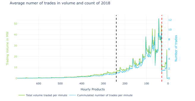
Figure 4: Visualization of the average number of trades per product, aggregated to minutely values, c.f. [14]. The left axis depicts the aggregated volume in MWh, while the right axis displays the number of trades in the minute. Regarding the case study, the left vertical line (black) shows the beginning of our trading interval, while the right vertical line (red) shows the end of the trading interval.

3.4 Detailed Description of the Environment

With the outlined restrictions, the trading environment $\mathbb{S}$ was constructed based on the methodology of Section 2.1. Hereby, the primary goal was to provide a trading environment that was close to the actual ID trade and incorporated most features. We followed the widely accepted Gym format of OpenAI [24] and again refer to Figure 1 for a better overview.

Episodes

To begin with, each hourly product was considered an individual episode in the environment. Depending on the scenario, the products were either randomly sampled (training) or processed sequential (testing). In the episode, the one minute volume weighted averages of the transaction price was computed. However, at some minutes no new observations were available, i.e., no new trade occurred, resulting in a forward passing of the previous price in order to ensure minutely coverage. As explained in the previous section, we fixed the number of trading steps to a length of 3.5 hours, thus each episode had a total of 211 time steps. Note that the agent had no influence on the completion of the episode, which differs from other DRL environments.

Action Space

For the action space $\mathbb{A}$ of the environment, we established a continuous action space, which should reflect the traded volume of the wind turbine on the electricity market. We restricted the operation margin, by setting lower and upper limits of MWh to our trading interval $a_{t}\ \in\ [0,1]$ for all $t\in T$. At each time step $t$, the agent adjusted through its action $a_{t}$ the traded volume and the difference $\Delta v_{t}=a_{t}-a_{t-1}$ thereafter was traded with the respective electricity price. With regard to the trading interval $a_{t}$, we decided to restrict the action for the following reasons. First, through only trading a maximum of one MWh, we could ensure that the price of the transaction was relatively similar to the LOB, as outlined in the previous section. Second, the interval simplified the interpretation of the results. Third, the forecasted wind volumes were also normalized within the interval [0,1], therefore the limit of $\mathbb{A}$ ensured a straightforward implementation.

Observation Space

The observation space of the DRL agent, i.e., the representation of the current state $s_{t}$, consisted of twelve features. We list the full table of our observation variables in Table 2 in the A. Next to the current price of the ID market $p_{t}$ and the forecast of the production volume $\eta_{t}$ (Section 3.5), ten additional features were included to increase the performance of the agent. These features can be differentiated in price variables, volume variables and episode variables and the most important ones are described below. The first important feature is the 5min-forecast of the electricity price $\hat{p}^{5min}_{t}$ (Section 3.5), which we introduce to indicate possible future trends for the agent. Further, we calculated the value of the portfolio by averaging the selling price in relation to the respective volume, denoted as $\tilde{p}^{port}_{t}$. With regard to the volume related variables, we included the current volume sold to the market, i.e., the previous action $a_{t-1}$ to ensure that the agent knows the available quantity for trading. In addition, we also included a difference between the current volume and the predicted production of the wind forecast, $vol_{diff}=\eta_{t}-a_{t-1}$. Lastly, we also added a distance measure that denotes the time until the trade ends $tte$, given that the variance of the ID price increases in the last minutes of the trade.

Reward

From the producer point of view, an increase in the trade volume would correspond to selling more capacity on the market and respectively a decrease in volume would correspond to buying back some electricity. Accordingly, we reflected this relation in the reward $r_{t}$ of the agent, which we defined for each time step $t$ as follows:

$$r_{t} =r_{t}^{vol}+r_{t}^{trade}.$$ (4)

As one can see, the reward was separated into two parts, with the first part being the trade reward $r_{t}^{trade}$ and the second the volume reward $r_{t}^{vol}$. The trade reward is valid for all time steps $t$ of the episode and is defined as follows:

$$\begin{aligned} r_{t}^{trade}&=p_{t}\Delta v_{t}-c_{fee}\mid\Delta v_{t}\mid,\\[5.0pt] \text{with}\ &\Delta v_{t}=a_{t}-a_{t-1}\end{aligned}$$ (5)

As one can see, $r_{t}^{trade}$ the denotes the selling/buying of the action difference $\Delta v_{t}$ to the current price $p_{t}$. Further, we also included a penalty for trading which reflects the transaction cost $c_{fee}$ and was set to 0.2€/MWh after consultation with industrial experts Thus, if $p_{t}>0.2$ an increase in volume (sold MWh) corresponds to a positive trade reward, while a decrease in volume (buy MWh) corresponds to a negative trade reward. Regarding the second part of the reward, the $r_{t}^{vol}$ is only computed in the last step of the episode $T$ and is defined as follows:

$$\begin{aligned} r_{t}^{vol}&=\left\{\begin{array}[]{lr}0&\ \text{for }t<T\\ -0.1\Delta v_{penalty}^{2}&\ \text{for }t=T\end{array}\right.,\\[12.0pt] \text{with }&v_{penalty}=\eta_{T}-a_{T}.\end{aligned}$$ (6)

The $r_{t}^{vol}$ is a penalty reward that measures the distance between the last action of the agent $a_{T}$ and the last provided wind forecast $\eta_{T}$. Through the quadratic term, the volume reward penalized large deviations, thus ensuring adaption at the end of the episode.

3.5 External Forecasts

In order to ensure a realistic trade behavior of the agent, we provided two forecasts in the observation space. The forecasts in question were on the one hand the wind power forecast of the wind farm $\eta_{t}$ and on the other hand a forecast of the next five minute price average $\hat{p}^{5min}_{t}$. In the following, we outline their structure shortly.

Intraday Price Forecast

The ID price forecast was constructed similar to the paper of [14], where both a Long Short-Term Memory (LSTM) and XGBoost model were used to predict future prices. Similar to [14], we used the XGBoost model for the forecast. However, contrary to cite [14] we decided to forecast the weighted ID price in 5min intervals, instead of 15min intervals. This has the advantage that short term changes are anticipated faster, however sacrificing at the cost of loosing mid-range information. In order to predict a specific month, the previous three months are considered as training interval. Note that we retrained the models for each new month to embed seasonal differences in the models. With regard to the input data, we included the transaction and LOB data of the EPEX SPOT market as well as the national wind forecast error of Germany.

Wind Forecast

In terms of the wind power forecast, we wanted to ensure a realistic setting by using a current state-of-the-art wind power prediction model. Therefore, we implemented an encoder-decoder Recurrent Neural Network (RNN) [33] for a multi-step-ahead forecast of the power generated by a single wind turbine. Encoder-decoder RNN consist of an encoder network that processes an input sequence and encodes it into a latent representation. The decoder network thereafter translates the encoded information to sequentially generate the output sequence, with each previously generated element influencing the next. Encoder-decoder RNN have been used several times in the literature for wind and solar power prediction [34]. In case of our analysis, we used an encoder consisting of an LSTM layer with 50 neurons. As a decoder, we used an LSTM layer with 50 neurons, followed by a dense layer with one neuron and a leaky ReLU activation function. The encoder received wind speed forecasts and wind power measurements from the past 28 hours as input. The decoder was initialized with the encoder’s hidden states. Further it received the wind power prediction of the previous prediction step such as the wind speed forecast of the current prediction step as input. The wind speed forecasts for the location of the wind turbine were extracted from the weather forecasts of the ICON-EU model, provided by the German Meteorological Service [35].

4 Case Study

4.1 Electricity Trading on the German ID Market of 2018

In this case study, we analyze the behavior of the DRL trading agent based on historic trading data from the German ID market. As primary data set the EPEX SPOT ID transaction data of 2018 was used for the trading environment, because the data was already available to the institute. With regard to trading regulations, we want to point out two market changes that happened in 2018. First, in June 2018 the XBID trading went live, which enables ID cross border trading [36]. Second, the German-Austrian bidding zone was separated in October 2018 into two different market areas [37]. Considering the impact of the first change, [8] found that the introduction of the XBID had no direct influence on the trading behavior, thus could be disregarded for market modeling. However, in terms of the market split we could not find similar analysis, thus decided to only selected the summer months of 2018 as our data set. In order to ensure impartial results, we proposed 10% of our data as out-of-sample test data, resulting in a training period from the 01.05.2018 till the 14.09.2018, with the remaining data 15.09-30.09.2018 as independent testing interval. The test interval represents the overall ID price of 2018 sufficiently and incorporate both products with average price distributions as well as outliers in the ID price. We present a more detailed analysis and comparison in the B. Further, to give a better overview, we display for each product the average ID price as well as the minimal/maximal outlier in Figure 5, with the testing interval underlined in red. As one can see, there are some extreme outliers in the data that might result in unstable training behavior. Consequently, training products with values above 150€ or below -50€ were discarded, which totals in 33 unregarded products. For the testing interval no products were filtered, given that these observations would not be known beforehand. Overall, we have in total 3.255 training and 384 testing products, which translates into 686.805 training and 81024 testing observation in our analysis.

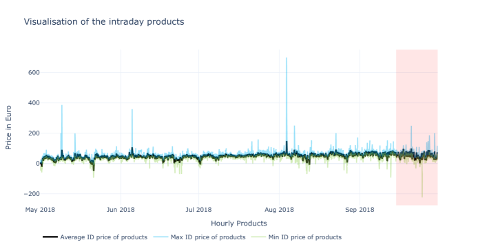
Figure 5: Plot of the 2018 German electricity ID price. Each product is visualized with its average, maximum and minimum value of the ID price. The training set is from May 2018 till mid of September, while the testing set is the remaining September (red).

4.2 Baseline Agents

As part of the case study, we want the agent to perform against different baseline agents to have an objective benchmark and asses the performance of the DRL agent correctly. However, some ground rules are necessary to ensure equal chances. First, all agents, including the DRL agent, had to start with a trading volume of 0 and could only trade in between the interval of [0,1] MWh. Further, to ensure physical delivery all agents were forced to end their trading on the last value of the wind forecast, which we corrected automatically at the end of each episode. Through fixing the start and end volume of the trading interval, we ensured a fair comparison, given that the performance was only depending on the movements within the trading interval.

With respect to the individual baseline agents, different approaches were chosen that should reflect different perspectives of the energy trading. The first and easiest agent $BL_{\text{First}}$ sold in the first step the volume according to the first wind forecasted volume $\eta_{0}$ at time $t_{0}$ without any other considerations. Then in the last step, it corrected the volume to the last predicted value of $\eta_{T}$. In conceptual terms, the second agent $BL_{\text{WF}}$ was constructed similar, because it strictly followed the wind volume forecast and traded every change (every 15 minutes) immediately. This agent therefore corresponds to a very conservative rule-based trading approach. The remaining agents are more sophisticated to reflect more complex approaches. The third agent $BL_{\text{PF}}$ is based on the ID price forecast values $\hat{p}^{5min}_{t}$ and should capture potential arbitrage possibilities. If for two sequential periods the difference between the price and the forecast indicated a smaller/larger energy price, the agents sold/bought a fixed proportion of its volume (0.1MWh) on the energy market. Our reasoning for proportional trading is that a higher proportion also induces higher transaction cost. Further, regarding the two sequential periods, we argue that the forecast $\hat{p}^{5min}_{t}$ is an average forecast for the next five minutes and hence captures a trend that might occur in later time steps. These constrains were experimentally found and showed better results than simply trading all capacities whenever the difference between forecast and price appeared. The last agent $BL_{\text{Random}}$ is a stochastic approach that should simulate a random behaviour on the ID market. With a probability of 25%, the baseline samples a new trading volume from a normal distribution. Thereby, the mean was the current wind forecast for the product, while the standard deviation was the standard deviation of the training data set. The 25% probability ensures that the agents performance is not to much influenced by the transaction costs of 0.2 €/MWh .

4.3 Experiment Metrics

For the comparison of the agents, we use multiple experiment metrics which we shortly introduce. First, we calculate the overall profit, which is the cumulative return across all test products, subtracted by the transaction costs (0.2€/MWh). Second, we derive a percentage performance in comparison to cumulative return of the $BL_{\text{WF}}$ baseline. Third, we present distributional properties with the mean, the standard deviation as well as the 10% and 90%Quantiles to give a better understanding of the allocation of the trading results. In addition, we were also interested in the best trade result, which the respective agent had in comparison to its peers. Therefore we return a relative measure in % in the results. Lastly, we conduct the average number of actions per product for the respective agent.

5 Results

5.1 Trading Results

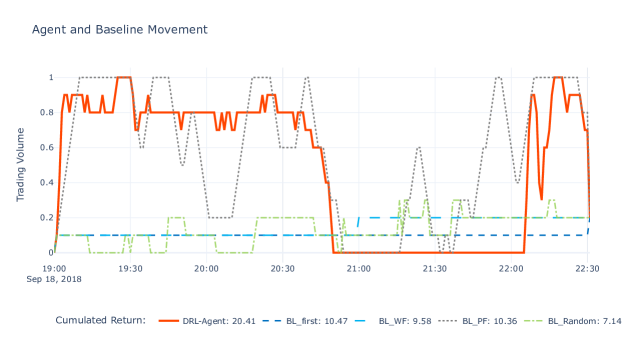
(a) Visualization of the baseline and DRL agent actions for the product of 2018-09-18 at 23.00. The trading period starts at 19.00 with a volume of 0 MWh and ends at 22.30 with a volume of 0.2MWh.

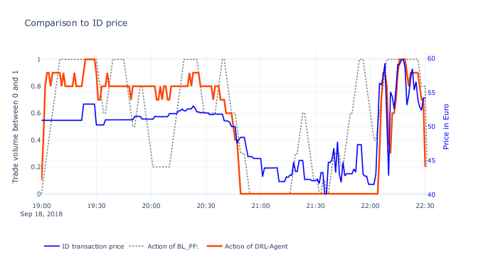
(b) This plot shows the actions of the DRL agent and $BL_{\text{PF}}$ in comparison to the ID price of the 2018-09-18 at 23.00 product. The left y-axis displays the trading volumes, while the right y-axis corresponds to the ID price.

Figure 6: Visualization of agent and baseline performance on the exemplary product 2018-09-18 at 23.00.

Based on the specifications of the case study, the results are shown in the following section. To begin with, we first present an exemplary product and thereafter analyze the overall results of the agents.

Exemplary Product

We selected an exemplary product 18.09.2018 at 23:00 UTC to visualize the actions of both agent and the baseline methods. In Figure 6 the respective actions are plotted, while in Figure 6(b) we plotted the price history of the product and compare it to the agent and $BL_{\text{PF}}$ action. Beginning with the baselines, one can see that both the $BL_{\text{First}}$ and $BL_{\text{WF}}$ were only trading twice, due to the minimal change in the wind forecast. Similarly, the $BL_{\text{Random}}$ had a relative narrow range in its movement, resulting in only a small deviation from the forecast. Consequently, all three agents had similar trade results.In contrast, the DRL-agent and $BL_{\text{PF}}$ had large changes in their trading action and use the full potential of their trading range. Both agents first sold all their available capacity in the first 30 minutes, re-bought when the price dropped (at around 20.45) and then again sold their capacity when the price was rising again. However, after 21.00 the $BL_{\text{PF}}$ started to sell parts of their capacity, while the agent seemed to anticipate future price trends and only moved after 22.05. Consequently, when looking at the Figure 6(b) one can see that the agent was exploiting the price drops at a lower price level than the $BL_{\text{PF}}$. Further, we want to draw the attention to the spike of the agent at 22:11, where the agent exploited the sudden plunge of the ID price. As a result, the agent was able to achieve a total return of 20.41€, whereas the $BL_{\text{PF}}$ only managed a total of 10.36€.

Overall Performance

While the visualization of a single product offers a first idea on the typical action range, we are naturally more interested in the overall trading results. Therefore, we visualize the performances across all products through a boxplot in Figure 7.

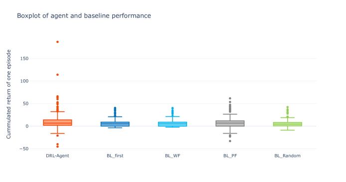
Figure 7: Box-plot of the performance from DRL agent and the baselines. The y-axis denotes the total return from each product of the test sample.

The first thing that becomes apparent is that both the DRL agent as well as the $BL_{\text{PF}}$ had a larger spread in their performance in comparison to the other more narrowly constructed baselines. This spread does not only correspond to higher trading values but also includes more negative and positive trading results. On the one hand, the DRL agent traded twice with a negative reward of -39.86€ and -45.27€. On the other hand, the agent was also able to achieve extraordinary returns with a maximum returns of 186.69€ and 114.00€.

	Agent	$BL_{\text{First}}$	$BL_{\text{WF}}$	$BL_{\text{PF}}$	$BL_{\text{Random}}$
Mean	9.72€	6.23€	6.15€	6.69€	5.50€
Median	6.86€	5.24€	5.26€	6.84€	4.59€
Standard Deviation	16.53€	6.42€	6.18€	10.47€	6.42€
10% Quantile	-1.01€	0.00€	0.00€	-4.73€	-0.79€
90% Quantile	23.88€	13.63€	13.45€	16.45€	12.65€
Total net profit	3731.69€	2390.85€	2360.56€	2569.22€	2111.08€
% Improvement to $BL_{WF}$	58.08%	1.28%	0.00%	8.84%	-10.57%
Best Performance in %	40.24%	15.48%	11.90%	28.57%	3.81%
Steps	27.95	1.08	1.34	77.89	26.59

Table 1: Trade results of the DRL agent and the baseline agents based on the performance metrics of Section 4.3.

Given that the one can not fully distinct between the median and quantiles of the boxplot, we report the performance metrics in the Table 1. Here, we can see that the DRL agent was in both mean and median better than the baselines, with the $BL_{\text{PF}}$ at second place, followed by the $BL_{\text{WF}}$, $BL_{\text{First}}$. The worst performance was the $BL_{\text{Random}}$, which was not surprising and shows that random behaviour does return sufficient results on the ID trade. Note that regarding the medians, the median of $BL_{\text{PF}}$ and the agent were quite similar. In addition, we are able to confirm the assumption that the agent and $BL_{\text{PF}}$ had a larger variance than the remaining baselines, which is both visible in the standard deviation as well as the quantiles. Naturally, when analysing trading methods one is primarily interested in the total net profit, where the agent was able to achieve the highest return with 3731.69€ and outperformed the $BL_{\text{WF}}$ by 58.08%. With comparison to the best baseline ($BL_{\text{PF}}$) this results to a surplus of 1162,47€. Considering the best performance per product, we see that the agent was able to achieve in 40.24% of times the best performance in direct comparison to the other baselines. Interestingly, the $BL_{\text{PF}}$ was following relatively close with 28.57%, while the remaining agents were clearly exceeded. Lastly, we consider the average number of steps per product, where the agent did an average of 27.95. In comparison to the 77.89 ($BL_{\text{PF}}$) and 26.59 ($BL_{\text{Random}}$) steps, these results conform the visual examination of the example product, where the agent had both some active trading intervals but also some times, where the action did not change.

5.2 Discussion and Future Outlook

Under consideration that this paper proposed a first attempt at a shortest-term trading DRL agent, we were able to show that it was indeed possible to apply DRL on the ID electricity trade in a minutely resolution. Even though the ID price emits a very high variance, the agent was able to identify patterns and create a sufficient trading strategy. This was primarily achieved through the development of the DRL environment. By excluding extreme outliers and implementing the necessary restrictions, we were able to create a training environment, which returned sufficient performance. The overall results clearly indicate an advantage through the DRL approach, considering that the agent outperformed all baselines, with best performances in 40.24% of the products. However, in comparison to the simple forecast of the $BL_{WF}$ and $BL_{first}$, we have to point out the higher variance in the trade results of the DRL agent. When looking at the highest negative return of the agent, i.e., the 2018-09-20 20:00:00 product with a -45.27€ loss, we observed that this product had large price increase up to 176.61€. The agent was not able to detect the price increase, which might partly be explained by the exclusion of extreme outliers from the training data. This might be a drawback for investors that are risk avers and do not want to anticipate negative results. Therefore, in future work one has to find a solution to cope with extreme outliers to ensure more stable results. Another deduction we have to make, is the role of the short-term price forecast. Its inclusion showed a clear increase in the agents performance and also returned better results in the $BL_{PF}$ baseline. Regarding the median results of the agent and $BL_{PF}$, there might be an indication that the average products can indeed be traded with the price forecast. However, for more volatile products the DRL agent provided a better trading strategy, resulting in overall better performance. Nevertheless, it will be interesting in future analysis, whether a more complex rule-based approach is able to achieve similar results than the agent. Lastly, given the limitations of our data, we want to address the fact that we evaluated the agent only on test data from one time period. On the one hand, the sample was a relative sufficient representation of the ID price from 2018, given that products with various price distributions were included, again see B. On the other hand, a two week period might not fully reflect possible long term influence, e.g., seasonal effects, that have an impact on the ID price. Therefore, to ensure reliable results, it will be necessary in future work to test the agent on large test samples as well as newer data. In this context, it might be interesting to enhance the performance through the inclusion of additional variables. One possible candidate could be the order book data, both as input variable as well as in the price mechanism. This would increase the complexity of the environment, considering that the bidding with orders and taking completed orders of the market needs to be included in the environment.

6 Conclusion

In this work, trading on the ID electricity market was formulated as a MDP in order to apply the DRL algorithms for autonomous trading. The novelty of the approach was the shortest-term resolution of one minute steps to depict the continuous trade. We offer multiple advancement to create a RL environment in which an DRL agent can train, while simultaneously remaining a realistic setting. The DRL environment was tested in a case study from the perspective of an electricity provider to manage a wind park with data from 2018. Our experiments show sufficient results with the agent outperforming the baselines by 45.24%. We discuss the implication of the results as well as limitations of our first approach and further offer possible enhancements for future research.

Appendix A Input Variables of Observation Space

In this section of the appendix, we present the underlying variables of the observation space to more detail.

Variable Group	Variables	Abbr. and Equation
Price Variables	Current and previous volume weighted electricity price	$p_{t},p_{t-1}$
	Day-ahead price	$P_{day_{a}head}$
	Forecast of electricity price	$\hat{p}^{5min}_{t}$
	Current and previous difference between price and forecast	$d_{t},d_{t-1}\text{ with }d_{t}=p_{t}-\hat{p}^{5min}_{t}$
	Portfolio price of the current volume	$\tilde{p}^{port}_{t}$
	Price Marker	$m=\left\{\begin{array}[]{lr}1&\ \text{for }d_{t}>0\text{and}d_{t-1}>0\\ -1&\ \text{for }d_{t}<0\text{and}d_{t-1}<0\\ 0&else\end{array}\right.$
Volume Variables	Forecast of the production volume from wind park	$\eta_{t}$
	Current volume of the trading agent	$a_{t-1}$
	Difference of current volume and production volume	$vol_{diff}$
Episode Variable	Time to end	$tte=1-\frac{t}{T}$

Table 2: Overview over the observation space variables. All variables are normalized in order to ensure stable training results. Note that the day ahead variable $P_{day_{a}head}$ is constant within each period and therefore has no time index.

Appendix B Testsample

As a test sample, 10% of the overall data was selected to validate the performance of the agents. We decided to use the products from 15.09.2018-30.09.2018 under consideration that these products represent the overall data sufficiently. In the test sample, the product 25.09.2018 records with -224.43€ the lowest ID price of 2018. Additionally, the products 2018-09-20 20:00:00 and 2018-09-29 19:00:00 are with their maximum values of 200€ and 249€ within the top 20 of the highest products of 2018. Therefore, they might offer some insight in the outlier behavior of the model. The appropriateness of the test data set can also be seen in Figure 8, where we visualize the overall ID prices of 2018 in comparison to the test interval. Generally, one can see that the test sample represents the product adequately, however small negative skewness in the tails is visible. Note that it is planned for future work to consider further training and testing periods to investigate the quality of the models.

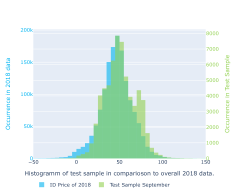
Figure 8: Histogram of the 2018 products in comparison to the products of the test sample. The overlap in the distribution can be seen as the dark green area in the histogram. Note that the different y-axis correspond to the frequency in the histogram-bins.

Appendix C Hyperparameter Selection

In this section of the appendix, the final hyperparameters of the PPO algorithm after the optimization with the PBT are presented. Thereafter, the hyperparameters of the wind and price forecast are displayed.

C.1 Hyperparameter PPO

Specification	Parameter	Value
Hyperparameter PPO	Clip parameter	0.432
	Entropy coefficient	0.001433
	Gamma	0
	KL coefficient	0.5
	Learning rate	0.0001
	SGD per iteration	7
	SGD minibatch size	422
	Train batch size	2532
	Value function clip parameter	10
	Value function loss coefficient	0.984103
	Shared value function layers	Yes
Network specification	First hidden layer units	64
	Second hidden layer units	64
	Third hidden layer units	32
	Activation function	Tanh

Table 3: Specifications and hyperparameter of PPO algorithm. The hyperparameters clip parameter, entropy coefficient,gamma, learning rate, SGD per iteration and value function loss coefficient were selected by the PBT algorithm.

C.2 Hyperparameter Price Forecast

Specification	Parameter	Value
Hyperparameter	Col-sample by tree	0.817699
	Gamma	0.097991
	Learning rate	0.043568
	Max depth	9
	N-estimators	184
	Sub sample	0.755471
Forecast Horizon	next 15min	3 x 5min
Forecast Update	Recalculation of the forecast	every 5min

Table 4: Forecast setting and hyperparameters of the XGBoost for the price forecast. The hyperparameters were selected through cross-validation of the training data.

C.3 Hyperparameter Wind Forecast

Specification	Parameter	Value
Model architecture	Layer Size Encoder	1
	Layer Size Decoder	1
	Hidden Layer Size Encoder	50
	Hidden Layer Size Encoder	50
Training Parameter	Learning rate	1e-4
	alpha	1e-5
	$l1_{ratio}$	0.1
	L1 regularization	$\text{alpha}*l1_{ratio}$
	L2 regularization	$\text{alpha}*(1-l1_{ratio})*0.5$
	Early stopping (patience)	5
	Mixed teacher forcing (dynamic reduction)	0.5-0.0
Training Specification	Training data	Prev. 2 months
	Validation data	Last 12,5% of training data
	Test data	Current month
Features	U-Component of wind	10m above the ground
	U-Component of wind	100m above the ground
	V-Component of wind	10m above the ground
	V-Component of wind	100m above the ground
Forecast horizon	4 hours	16 x 15min
Forecast update	Recalculation of forecast	Every 15min

Table 5: Forecast settings and hyperparameters of the wind forecast model.

References

- [1] European Comission, The european green deal, https://eur-lex.europa.eu/legal-content/EN/TXT/PDF/?uri=CELEX:52019DC0640&from=EN (Accessed: 2021-10-27).
- [2] IEA (2021), Global energy review 2021, https://www.iea.org/reports/global-energy-review-2021 (Accessed: 2021-10-27).
- [3] R. Kiesel, F. Paraschiv, Econometric analysis of 15-minute intraday electricity prices, Energy Economics 64 (2017) 77–90. doi:10.1016/j.eneco.2017.03.002.
- [4] P. Shinde, M. Amelin, A literature review of intraday electricity markets and prices, in: 2019 IEEE Milan PowerTech, 2019, pp. 1–6. doi:10.1109/PTC.2019.8810752.
- [5] EPEX SPOT, New record volume traded on epex spot in 2020, https://www.epexspot.com/en/news/new-record-volume-traded-epex-spot-2020 (Accessed: 2021-10-27).
- [6] F. Ziel, Modeling the Impact of Wind and Solar Power Forecasting Errors on Intraday Electricity Prices, in: 2017 14th International Conference on the European Energy Market (EEM), 2017, pp. 1–5. doi:10.1109/EEM.2017.7981900.
- [7] C. Koch, L. Hirth, Short-term electricity trading for system balancing: An empirical analysis of the role of intraday trading in balancing germany’s electricity system, Renewable and Sustainable Energy Reviews 113 (2019) 109275.
- [8] C. Kath, Modeling Intraday Markets Under the New Advances of the Cross-Border Intraday Project (XBID): Evidence from the German Intraday Market, Energies 12 (2019) 4339. doi:10.3390/en12224339.
- [9] C. Pape, S. Hagemann, C. Weber, Are Fundamentals Enough? Explaining Price Variations in the German Day-Ahead and Intraday Power Market, Energy Economics 54 (2016) 376–387. doi:10.1016/j.eneco.2015.12.013.
- [10] M. Narajewski, F. Ziel, Econometric Modelling and Forecasting of Intraday Electricity Prices, Journal of Commodity Markets (2019) 100107doi:10.1016/j.jcomm.2019.100107.
- [11] M. Narajewski, F. Ziel, Ensemble forecasting for intraday electricity prices: Simulating trajectories, Applied Energy 279 (2020) 115801.
- [12] B. Uniejewski, G. Marcjasz, R. Weron, Understanding Intraday Electricity Markets: Variable Selection and very Short-Term Price Forecasting Using LASSO, International Journal of Forecasting 35 (2019) 1533–1547. doi:10.1016/j.ijforecast.2019.02.001.
- [13] T. Janke, F. Steinke, Forecasting the price distribution of continuous intraday electricity trading, Energies 12 (22) (2019) 4262.
- [14] C. Scholz, M. Lehna, K. Brauns, A. Baier, Towards the prediction of electricity prices at the intraday market using shallow and deep-learning methods, in: Workshop on Mining Data for Financial Applications, Springer, 2020, pp. 101–118.
- [15] W. Wang, N. Yu, A machine learning framework for algorithmic trading with virtual bids in electricity markets, in: 2019 IEEE Power & Energy Society General Meeting (PESGM), IEEE, 2019, pp. 1–5.
- [16] S. Baltaoglu, L. Tong, Q. Zhao, Algorithmic bidding for virtual trading in electricity markets, IEEE Transactions on Power Systems 34 (1) (2018) 535–543.
- [17] Y. Ye, D. Qiu, M. Sun, D. Papadaskalopoulos, G. Strbac, Deep reinforcement learning for strategic bidding in electricity markets, IEEE Transactions on Smart Grid 11 (2) (2019) 1343–1355.
- [18] N. Rashedi, M. A. Tajeddini, H. Kebriaei, Markov game approach for multi-agent competitive bidding strategies in electricity market, IET Generation, Transmission & Distribution 10 (15) (2016) 3756–3763.
- [19] H. Xu, H. Sun, D. Nikovski, S. Kitamura, K. Mori, H. Hashimoto, Deep reinforcement learning for joint bidding and pricing of load serving entity, IEEE Transactions on Smart Grid 10 (6) (2019) 6366–6375.
- [20] H. Wang, B. Zhang, Energy storage arbitrage in real-time markets via reinforcement learning, in: 2018 IEEE Power & Energy Society General Meeting (PESGM), IEEE, 2018, pp. 1–5.
- [21] G. Bertrand, A. Papavasiliou, An analysis of threshold policies for trading in continuous intraday electricity markets, in: 2018 15th International Conference on the European Energy Market (EEM), IEEE, 2018, pp. 1–5.
- [22] I. Boukas, D. Ernst, A. Papavasiliou, B. Cornélusse, Intra-day bidding strategies for storage devices using deep reinforcement learning, in: International Conference on the European Energy Market, Łódź 27-29 June 2018, 2018, p. 6.
- [23] G. Bertrand, A. Papavasiliou, Reinforcement-learning based threshold policies for continuous intraday electricity market trading, in: 2019 IEEE Power & Energy Society General Meeting (PESGM), IEEE, 2019, pp. 1–5.
- [24] G. Brockman, V. Cheung, L. Pettersson, J. Schneider, J. Schulman, J. Tang, W. Zaremba, Openai gym (2016). arXiv:arXiv:1606.01540.
- [25] R. S. Sutton, D. A. McAllester, S. P. Singh, Y. Mansour, et al., Policy gradient methods for reinforcement learning with function approximation., in: NIPs, Vol. 99, Citeseer, 1999, pp. 1057–1063.
- [26] V. Mnih, K. Kavukcuoglu, D. Silver, A. A. Rusu, J. Veness, M. G. Bellemare, A. Graves, M. Riedmiller, A. K. Fidjeland, G. Ostrovski, et al., Human-level control through deep reinforcement learning, nature 518 (7540) (2015) 529–533.
- [27] T. P. Lillicrap, J. J. Hunt, A. Pritzel, N. Heess, T. Erez, Y. Tassa, D. Silver, D. Wierstra, Continuous control with deep reinforcement learning, arXiv preprint arXiv:1509.02971 (2015).
- [28] J. Schulman, F. Wolski, P. Dhariwal, A. Radford, O. Klimov, Proximal policy optimization algorithms, arXiv preprint arXiv:1707.06347 (2017).
- [29] V. Mnih, A. P. Badia, M. Mirza, A. Graves, T. Lillicrap, T. Harley, D. Silver, K. Kavukcuoglu, Asynchronous methods for deep reinforcement learning, in: International conference on machine learning, PMLR, 2016, pp. 1928–1937.
- [30] D. P. Kingma, J. Ba, Adam: A method for stochastic optimization, arXiv preprint arXiv:1412.6980 (2014).
- [31] M. Jaderberg, V. Dalibard, S. Osindero, W. M. Czarnecki, J. Donahue, A. Razavi, O. Vinyals, T. Green, I. Dunning, K. Simonyan, et al., Population based training of neural networks, arXiv preprint arXiv:1711.09846 (2017).
- [32] H. Martin, S. Otterson, German intraday electricity market analysis and modeling based on the limit order book, in: 2018 15th International Conference on the European Energy Market (EEM), IEEE, 2018, pp. 1–6.
- [33] I. Sutskever, O. Vinyals, Q. V. Le, Sequence to sequence learning with neural networks, in: Advances in neural information processing systems, 2014, pp. 3104–3112.
- [34] G. Alkhayat, R. Mehmood, A review and taxonomy of wind and solar energy forecasting methods based on deep learning, Energy and AI (2021) 100060.
- [35] Deutscher Wetterdienst, Icon database reference manual, https://www.dwd.de/SharedDocs/downloads/DE/modelldokumentationen/nwv/icon/icon_dbbeschr_aktuell.pdf (Accessed: 2021-09-29).
- [36] EPEX SPOT, Epex spot annual market review 2018, https://www.epexspot.com/en/news/traded-volumes-soar-all-time-high-2018 (Accessed: 2021-11-02).
- [37] EPEX SPOT, Epex spot to publish separate prices and volumes for the austrian and german day-ahead markets, https://www.epexspot.com/en/news/epex-spot-publish-separate-prices-and-volumes-austrian-and-german-day-ahead-markets (Accessed: 2021-11-02).