Microscopical Justification of the Winterbottom problem for well-separated Lattices

Abstract.

We consider the discrete atomistic setting introduced in [25] to microscopically justify the continuum model related to the Winterbottom problem, i.e., the problem of determining the equilibrium shape of crystalline film drops resting on a substrate, and relax the rigidity assumption considered in [25] to characterize the wetting and dewetting regimes and to perform the discrete to continuum passage. In particular, all results of [25] are extended to the setting where the distance between the reference lattices for the film and the substrate is not smaller than the optimal bond length between a film and a substrate atom. Such optimal film-substrate bonding distance is prescribed together with the optimal film-film distance by means of two-body atomistic interaction potentials of Heitmann-Radin type, which are both taken into account in the discrete energy, and in terms of which the wetting-regime threshold and the effective expression for the wetting parameter in the continuum energy are determined.

1. Introduction

In this manuscript we address the classical problem of determining the equilibrium shape formed by crystalline film drops resting upon rigid substrates possibly of a different material. Such problem has a variational nature as the solution can be looked for among the minimizers of a surface energy that depends both on the drop anisotropy at the drop surface and on the drop wettability at the contact region with the flat substrate. By exploiting the interplay between the drop anisotropy and wettability W. L. Winterbottom provided in [29] the first phenomenological prediction of the solution by a direct construction of the nowadays called Winterbottom shape (see Figure 1). We intend here to move forward from the results obtained by the authors in [25] by extending the discrete to continuum derivation of the energy considered by Winterbottom (see also [15, 16]) established in [25] to all mutual positionings of the reference lattices of the film and of the substrate, whose distance is not smaller than the optimal bond distance between a film and a substrate atom.

More precisely, the energy considered by W. L. Winterbottom in the continuum planar setting in [15, 16, 29] expressed in modern terminology is defined for any set of finite perimeter $D\subset\mathbb{R}^{2}\setminus S$ representing the area occupied by a film drop outside of the substrate region $S\subset\mathbb{R}^{2}$ by

$$\mathcal{E}(D):=\int_{\partial^{*}D\setminus\partial S}\Gamma(\nu(\xi))\,\mathrm{d}\mathcal{H}^{1}(\xi)+\sigma\mathcal{H}^{1}(\partial^{*}D\cap\partial S),$$ (1)

where $\Gamma:\mathbb{S}^{1}\to\mathbb{R}$ is the anisotropic surface tension related to the material of the crystalline drop and defined on the normal $\nu\in\mathbb{S}^{1}$ at the reduced boundary $\partial^{*}D$, while $\sigma\in\mathbb{R}$ is a parameter representing the wetting, namely, the ability of the drop to maintain contact with the specific solid surface $\partial S$, which is the topological boundary of $S$, and $\mathcal{H}^{1}$ is the 1-dimensional Hausdorff measure (see 2.6 for more details). By adapting the phenomenological construction provided by G. Wulff in [30] of the set, nowadays named after him, for the related problem of finding the equilibrium shape of a free-standing crystal with anisotropy $\Gamma$ in the space, i.e., for the minimizer of (1) in the case with $S=\emptyset$ (see also [10, 12]), that is

$$W_{\Gamma}:=\{x\in\mathbb{R}^{d}\,:\,x\cdot\nu\leq\Gamma(\nu)\text{ for every }\nu\in S^{d-1}\},$$

the Winterbottom shape for the flat substrate $S=\mathbb{R}\times\{s\in\mathbb{R}\,:\,s<0\}$ is the set

$$W_{\Gamma,\sigma}:=W_{\Gamma}\cap\{x\in\mathbb{R}^{d}\,:\,x_{d}\geq-\sigma\},$$

as depicted in Figure 1.

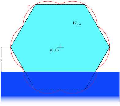
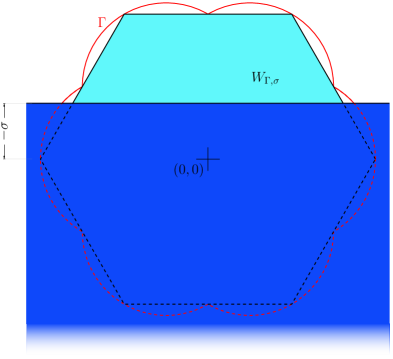
Figure 1. Winterbottom construction for the minimizer of $\mathcal{E}$, on the left for $\sigma>0$ and on the right for $\sigma<0$ (see [29]).

For the justification of the problem in dimension $d=2$ in the context of statistical mechanics and the Ising model we refer to the review [9] (see also [14, 17]) for the Wulff shape in the scaling limit at low-temperature and to [4, 23, 24] for the setting related to the Winterbottom shape, while in the context of atomistic models a rigorous discrete to continuum passage for triangular reference lattices has been first carried out by means of $\Gamma$-convergence in [2] for the Wulff shape and then extended to the Winterbottom situation in [25]. The emergence of the Wulff shape has been also deduced for the square lattice in [20, 21] and the hexagonal lattice [7] by means of a different approach based on induction techniques related to the crystallization problem [13], and of the quantification of the deviation of discrete ground states from the asymptotic Wulff shape in the so called $n^{3/4}$ law (where $n$ is the number of atoms), which was previously introduced in [26], and then extended to those settings (see also [8]), and more recently to higher dimensions in [19, 22]. A derivation by $\Gamma$-convergence of an energy of the type (1) coupled with a bulk elastic term in the context of models for epitaxially-strained thin films introduced in [5, 6, 11, 27, 28] has been instead determined in [18] under a graph constraint for the region occupied by the film drop.

We follow the approach of [25], where the authors introduced a specific discrete setting, which here we intend to generalize, to initiate the analysis for the Winterbottom problem in the context of atomistic models by taking into consideration not only atomistic interactions among each other film atoms as in [2], but also between film and substrate atoms, in terms of two-body potentials $v_{F,\alpha}$ of Heitmann-Radin sticky-disc type [13] with $\alpha=F,S$ for film-film and film-substrate atomistic interactions, respectively. More precisely, in [25] the discrete setting involves a reference lattice $\mathcal{L}_{S}\subset\overline{S}:=\mathbb{R}\times\{s\in\mathbb{R}\,:\,s\leq 0\}$ for the substrate atoms, which is assumed to be fully occupied, and a triangular reference lattice $\mathcal{L}_{F}\subset\mathbb{R}^{2}\setminus\overline{S}$ defined by

$$\mathcal{L}_{F}:=\{x_{F}+k_{1}\bm{t}_{1}+k_{2}\bm{t}_{2}\,:\,\color[rgb]{0,0,0}\textrm{$k_{1}\in\mathbb{Z}$ and $k_{2}\in\mathbb{N}\cup\{0\}$}\color[rgb]{0,0,0}\}$$

for a fixed $x_{F}\in\mathbb{R}^{2}\setminus\overline{S}$, which we call film-lattice center,

$$\bm{t}_{1}:={1\choose 0},\quad\textrm{and}\quad\bm{t}_{2}:=\color[rgb]{0,0,0}\frac{1}{2}{1\choose\sqrt{3}},$$

on which film atoms are free to choose the most convenient configuration under the considered atomistic interactions $v_{F,\alpha}$ with $\alpha=F,S$. Thus, for each fixed number $n\in\mathbb{N}$ all sets $D_{n}:=\{x_{1},\ldots,x_{n}\}\subset\mathcal{L}_{F}$ are considered admissible configurations of $n$ film atoms (see Figure 2), and the overall energy $V_{n}:(\mathbb{R}^{2}\setminus\overline{S})^{n}\to\mathbb{R}\cup\{\infty\}$ of a configuration $D_{n}:=\{x_{1},\ldots,x_{n}\}\subset\mathcal{L}_{F}$ is defined by

$$V_{n}(D_{n})=V_{n}(x_{1},\ldots,x_{n}):=\sum_{i\neq j}v_{FF}(|x_{i}-x_{j}|)\,+\,\sum_{i=1}^{n}\sum_{s\in\partial\mathcal{L}_{S}}v_{\textrm{FS}}(|x_{i}-s|),$$

where the sums are extended to nearest neighbors and $\partial\mathcal{L}_{S}:=\mathcal{L}_{S}\cap\mathbb{R}\times\{s\in\mathbb{R}\,:\,s=0\}$ is referred to as the substrate surface or wall. Notice that in [25] the minimum of the atomistic potentials $v_{F\alpha}$ is fixed at $e_{F\alpha}>0$ with values $-c_{\alpha}<0$ for $\alpha=F,S$, respectively. where $e_{FF}$ is normalized at 1 and coincide with the lattice parameter of $\mathcal{L}_{F}$, while the following rigidity assumption was made in regard of $e_{FS}$:

$$\text{$x_{F}:=x_{F}^{0}$\quad with\quad$x_{F}^{0}:=(0,e_{FS})$},$$ (2)

which in particular by the choice of $\partial\mathcal{L}_{S}$ was preventing the possibility of two substrate neighbors for film atoms (which is the maximum possible number of substrate neighbors for the situation with a flat substrate and a Heitmann-Radin potential $v_{FS}$).

The aim of this manuscript is to relax the rigidity assumption (2) and obtain the full generality of the results in [25] for all the positionings $x_{F}\in\mathbb{R}^{2}\setminus\overline{S}$ for $\mathcal{L}_{F}$ for which

$${\rm dist}(\partial\mathcal{L}_{F},\partial\mathcal{L}_{S})\geq e_{FS}$$ (3)

(which include (2)) and hence, in particular allowing film atoms (resp. substrate atoms) to display from zero to two substrate neighbors (resp. film neighbors).

The results are threefold (see Section 2.7): First, we characterize in Theorem 2.3 the wetting regime, i.e., when film atoms are expected to spread on the substrate surface instead of accumulating in island clusters on top of it, in terms of the parameters $c_{\alpha}$ related to the atomistic potentials $v_{F\alpha}$ for $\alpha=F,S$. Furthermore, also the corresponding minimizers in such regime are explicitly isolated for every $n\in\mathbb{N}$ by induction techniques related to crystallization problems (see, e.g., [13, 20]). In particular, as a result of the much more involved setting an extra threshold condition under which the film spreads in an infinitesimally thick layer is found for certain settings in between the thresholds already determined in [25].

Second, we prove in Theorem 2.4 that in the dewetting regime, where film atoms are expected to form solid-state islands (related to regions with positive two-dimensional Lebesgue measure $\mathcal{L}^{2}$), the mass of the solutions of the discrete minimum problems

$$\min_{D_{n}\subset\mathcal{L}_{F}}{V_{n}(D_{n})}\$$ (4)

as the number $n$ of atoms tends to infinity does not spread, but up to a subsequence it is preserved by the connected components of such minimizers with largest cardinality. This is crucial to overcome the lack of compactness that we have, as already detailed in [25], outside the class of almost-connected configurations, which are roughly speaking, configurations connected up to a substrate-bond distance (see Section 2.2 for more details).

Finally, we establish in Theorem 2.5 that in the dewetting regime the solutions of the discrete problems (4) converge as the number $n$ of film atoms tends to infinity (up to extracting a subsequence and performing horizontal translations on the substrate $S$) to a minimizer of the Winterbottom energy (1) in the family of crystalline-drop regions

$$\mathcal{D}_{\rho}:=\{D\subset\mathbb{R}^{2}\setminus S\,:\,\text{set of finite perimeter, bounded and such that $|D|=1/\rho$}\},$$

where $\rho$ is the atom density in $\mathcal{L}_{F}$ per unit area. This convergence of the discrete minimizers in the dewetting regime is obtained in view of the conservation of mass proven of Theorem 2.4 by following the approach in [2, 25] and proving the $\Gamma$-convergence as $n\to\infty$ of properly defined (and rescaled) versions of $V_{n}$ in the space $\mathcal{M}(\mathbb{R}^{2})$ of Radon measures on $\mathbb{R}^{2}$ with respect to the weak* convergence of measures. In particular, an effective expression for the wetting parameter $\sigma$ in (1) is obtained, i.e.,

$$\sigma:=\begin{cases}2c_{F}-\displaystyle\frac{2c_{S}}{q}&\text{for $C_{i}$ with $i=1,3,4$,}\\ &\\ 2c_{F}-\displaystyle\frac{c_{S}}{q}&\text{for $C_{2}$,}\\ \end{cases}$$ (5)

where $q\in\mathbb{N}$ relates to the optimal substrate bond $e_{S}:=q/p$ in $\partial\mathcal{L}_{S}$ with $p\in\mathbb{N}$, and $C_{i}$ with $i=1,\dots,4$ are categories in which the various settings allowed by (3) can be classified (see Section 2.7 for more details).

Our methodology consists in introducing a more general setting (even more general of the settings described above) with substrate wall

$$\partial\mathcal{L}_{S}=\left\{s_{k}:=\left(\frac{k}{p},0\right)\,:\,k\in q\mathbb{Z}\cup\left(q\mathbb{Z}+r\right)\right\}$$ (6)

for wall parameters $z:=(p,q,r)\in Z_{S}$ with

$$Z_{S}:=\left\{(p,q,r)\in\mathbb{N}\times\mathbb{N}\times\mathbb{N}_{0}:\text{$p$ and $q$ co-prime, $0\leq r\leq\frac{q}{2}$, and $p=1$ if $r\neq 0$}\right\}$$

where $\mathbb{N}_{0}:=\mathbb{N}\cup\{0\}$, which reduces to the relevant settings described above for

$$z\in Z_{S}^{0}:=\{(p,q,r)\in Z_{S}:r=0\}$$

(and in particular to the model of [25] for $x_{F}:=x_{F}^{0}$ and $z\in Z_{S}^{0}$) and to an extra auxiliary setting for $z\in Z_{S}^{1}:=Z_{S}\setminus Z_{S}^{0}$. Such an auxiliary setting is carefully determined in order to both be able to implement all the program of [25] for it as well, and as the only extra needed model for treating all the settings with $z\in Z_{S}^{0}$ that cannot be reduced to the model in [25]. More precisely, we introduce an equivalence relation among the various possible settings with substrate wall (6) and prove that all the settings with $z\in Z_{S}^{0}$ satisfying (3) can be reduced either to the model of [25] or to the auxiliary model with $z\in Z_{S}^{1}$. Since in particular such equivalence relation preserves all the properties contained in the main results, we are then allowed to transfer such properties from the model already treated in [25] and from the auxiliary model, by directly proving them extra only for the latter.

More specifically, the classes $C_{i}$ with $i=1,\dots,4$ for the various settings with $z\in Z_{S}^{0}$ are exactly introduced to prove the equivalence to the two specific setting: the settings in classes $C_{i}$ for $i=1,\dots,3$ are equivalent to the model in [25] (with different lattice parameters) and the settings in the class $C_{4}$ to the auxiliary model introduced in this manuscript. Moreover, a specific feature of the auxiliary model for $z\in Z_{S}^{1}$ is the possibility of having separated pairs of film atoms bonded with the substrate. To accommodate such aspect in the strategy of [25] we need to include the extra wetting condition appearing in Theorem 2.3, extend the strip argument used to establish the compactness for almost-connected configurations used to prove the conservation of mass of Theorem 2.4 (see the more involved definition for the strip energy in Section 2.4), and finally adjust the “boundary-averaging” arguments used for the lower bound in the proof of the $\Gamma$-convergence, which in turns is responsible for the more involved form of the effective expression for the wettability $\sigma$ in (5) with respect to [25].

The paper is organized as follows. In Section 2 we introduce the mathematical setting and the main results of the paper. In Section 3 we implement the program of [25] for the auxiliary model with substrate wall $\partial\mathcal{L}_{S}$ of the type (6) with $z\in Z_{S}^{1}$. In Section 4 we prove the equivalence property for each class $C_{i}$ with $i=1,\dots,4$ of settings satisfying (3) and the main results of the paper.

2. Mathematical setting and main results

In this section we introduce the discrete and continuous models, the notation and definitions used throughout the paper, and the main results.

2.1. Setting with lattice configurations

We begin by introducing a reference set $\mathcal{L}$ for the atoms of the substrate and of the film in the plane $\mathbb{R}^{2}$ for a chosen cartesian coordinate system. We define $\mathcal{L}:=\mathcal{L}_{S}\cup\mathcal{L}_{F}$, where $\mathcal{L}_{S}\subset\overline{S}$ denotes the reference lattice for the substrate atoms, with $S:=\mathbb{R}\times\{s\in\mathbb{R}\,:\,s<0\}$ referred to as the substrate region, and $\mathcal{L}_{F}\subset\mathbb{R}^{2}\setminus\overline{S}$ is the reference lattice for the film atoms.

More precisely, we consider the substrate lattice as a fixed set, i.e., every lattice site in $\mathcal{L}_{S}$ is occupied by a substrate atom, such that

$$\partial\mathcal{L}_{S}:=\mathcal{L}_{S}\cap\{(s,0):\,s\in\mathbb{R}\,\}=\left\{s_{k}:=\left(\frac{k}{p},0\right)\,:\,k\in q\mathbb{Z}\cup\left(q\mathbb{Z}+r\right)\right\}$$ (7)

for $z:=(p,q,r)\in Z_{S}$ with

$$Z_{S}:=\left\{(p,q,r)\in\mathbb{N}\times\mathbb{N}\times\mathbb{N}_{0}:\text{$p$ and $q$ co-prime, $0\leq r\leq\frac{q}{2}$, and $p=1$ if $r\neq 0$}\right\}$$

where $\mathbb{N}_{0}:=\mathbb{N}\cup\{0\}$. We refer to $\partial\mathcal{L}_{S}$ as to the substrate wall (or substrate surface) and the vectors $z=(p,q,r)\in Z_{S}$ as the wall vector with wall parameters $p$, $q$, and $r$. We notice that we choose such a definition for $\partial\mathcal{L}_{S}$ even though it could be simplified, in order to directly include the setting used in [25] without inconsistent notation between the two papers. Furthermore, notice that the choice of wall vectors $z=(1,q,r)$ with $q/2<r\leq q$ are excluded in the definition of $Z_{S}$ without loss of generality up to a translation of the origin in the $\bm{t}_{1}$ direction.

For the film lattice $\mathcal{L}_{F}$ we choose a triangular lattice with parameter $e_{F}$ normalized to 1 (with respect to the wall parameters), namely

$$\mathcal{L}_{F}:=\{x_{F}+k_{1}\bm{t}_{1}+k_{2}\bm{t}_{2}\,:\,\color[rgb]{0,0,0}\textrm{$k_{1}\in\mathbb{Z}$ and $k_{2}\in\mathbb{N}\cup\{0\}$}\color[rgb]{0,0,0}\}$$ (8)

for

$$\bm{t}_{1}:={1\choose 0},\quad\textrm{and}\quad\bm{t}_{2}:=\color[rgb]{0,0,0}\frac{1}{2}{1\choose\sqrt{3}},$$

and

$$x_{F}:=(x_{F}^{1},x_{F}^{2})\in\mathbb{R}^{2}\setminus\overline{S},$$

which we refer to as the film-lattice center. Let also $\bm{t}_{3}$ be

$$\bm{t}_{3}:={0\choose 1}.$$

The sites of the film lattice are not assumed to be completely filled and we refer to a set of $n\in\mathbb{N}$ sites $x_{1},\dots,x_{n}\in\mathcal{L}_{F}$ occupied by film atoms as a crystalline configuration denoted by $D_{n}:=\{x_{1},\dots,x_{n}\}\subset\mathcal{L}_{F}$. Notice that the labels for the elements of a configuration $D_{n}$ are uniquely determined by increasingly assigning them with respect to a chosen fixed order on the lattice sites of $\mathcal{L}_{F}$. With a slight abuse of notation we refer to $x\in D_{n}$ as an atom in $D_{n}$ (or in $\mathcal{L}_{F}$). We denote the family of crystalline configurations with $n$ atoms by $\mathcal{C}_{n}$. Furthermore, given a set $A\subset\mathbb{R}^{2}$, its cardinality is indicated by $\#A$, so that

$$\mathcal{C}_{n}:=\{A\subset\mathcal{L}_{F}\,:\,\#A=n\}.$$

For every atom $x\in\mathcal{L}_{F}$ we take into account both its atomistic interactions with other film atoms and with the substrate atoms, by considering the two-body atomistic potentials $v_{FF}$ and $v_{FS}$, respectively. We restrict to first-neighbor interactions and we define $v_{F\alpha}$ for $\alpha:=F,S$ as

$$v_{F\alpha}(s):=\begin{cases}+\infty&\mbox{if }s<e_{F\alpha},\\ -c_{\alpha}&\mbox{if }s=e_{F\alpha},\\ 0&\mbox{if }s>e_{F\alpha},\end{cases}$$ (9)

with $c_{\alpha}>0$, $e_{FF}:=e_{F}=1$, and $e_{FS}>0$.

We denote by $\partial\mathcal{L}_{F}$ the lower boundary of the film lattice, i.e.,

$$\partial\mathcal{L}_{F}:=\{x_{F}+k_{1}\bm{t}_{1}:\,\color[rgb]{0,0,0}\textrm{$k_{1}\in\mathbb{Z}$}\color[rgb]{0,0,0}\}$$

and by $\partial\mathcal{L}_{FS}$ the collection of sites in the lower boundary of the film lattice at a distance of $e_{FS}$ from an atom in $\partial\mathcal{L}_{S}$, i.e.,

$$\partial\mathcal{L}_{FS}:=\partial\mathcal{L}_{F}\cap\{x\in\mathbb{R}^{2}:{\rm dist}(x,\partial\mathcal{L}_{S})=e_{FS}\}.$$

In the following, we refer to film and substrate neighbors of an atom $x$ in a configuration $D_{n}$ as to those atoms in $D_{n}$ at distance 1 from $x$, and to those atoms in $\mathcal{L}_{S}$ at distance $e_{FS}$ from $x$, respectively. Analogously, we refer to film and substrate bonds of an atom $x$ in a configuration $D_{n}$ as to those segments connecting $x$ to its film and substrate neighbors, respectively. More generally the same terminology will be extended for sites of $\mathcal{L}_{F}$. We also refer to the union of the closures of all film bonds of atoms in a configuration $D_{n}$ as the bonding graph of $D_{n}$, and we say that a crystalline configuration $D_{n}$ is connected if every $x$ and $y$ in $D_{n}$ are connected through a path in the bonding graph of $D_{n}$, i.e., there exist $\ell\leq n$ and $x_{k}\in D_{n}$ for $k:=1,\dots,\ell$ such that $|x_{k}-x_{k-1}|=1$, $x_{1}=x$, and $x_{\ell}=y$. Moreover, we define the boundary of a configuration $D_{n}\in\mathcal{C}_{n}$ as the set $\partial D_{n}$ of atoms of $D_{n}$ with less than 6 film neighbors. We notice here that with a slight abuse of notation, given a set $A\subset\mathbb{R}^{2}$ the notation $\partial A$ will also denote the topological boundary of a set $A\subset\mathbb{R}^{2}$ (which we intend to be always the way to interpret the notation when applied not to configurations in $\mathcal{C}_{n}$, or to lattices, such as for $\partial\mathcal{L}_{S}$, $\partial\mathcal{L}_{F}$, and $\partial\mathcal{L}_{FS}$).

The energy $V_{n}$ of a configuration $D_{n}:=\{x_{1},\ldots,x_{n}\}\subset\mathcal{L}_{F}$ of $n$ particles is defined by

$$\color[rgb]{0,0,0}V_{n}(D_{n})=\color[rgb]{0,0,0}V_{n}(x_{1},\ldots,x_{n})\color[rgb]{0,0,0}:=\color[rgb]{0,0,0}\sum_{i\neq j}v_{FF}(|x_{i}-x_{j}|)\,+\,E_{S}(x_{1},\ldots,x_{n})\color[rgb]{0,0,0}$$ (10)

where $E_{S}:(\mathbb{R}^{2}\setminus\overline{S})^{n}\color[rgb]{0,0,0}\to\mathbb{R}\cup\{\infty\}$ represents the overall contribution of the substrate interactions defined as

$$E_{S}(D_{n})=E_{S}(x_{1},\dots,x_{n}):=\sum_{i=1}^{n}v^{1}(x_{i}),$$ (11)

where the one-body potential $v^{1}$ is defined by

$$v^{1}(x):=\sum_{s\in\mathcal{L}_{S}}v_{\textrm{FS}}(|x-s|)$$ (12)

for any $x\in\mathbb{R}\times\{r\in\mathbb{R}\,:\,r>0\}$. Notice that from the definition of $v_{FS}$ and $x_{F}$

$$v^{1}(x)\in\{\infty,0,-c_{S},-2c_{S}\}$$

for any $x\in\mathcal{L}_{F}$.

Furthermore, we considered the setting from the Introduction with (3), i.e.,

$${\rm dist}(\partial\mathcal{L}_{F},\partial\mathcal{L}_{S})\geq e_{FS},$$ (13)

but without loss of generality we can actually reduce to the setting

$$\partial\mathcal{L}_{FS}\neq\emptyset$$ (14)

(which implies the equality in (13)) since otherwise by the choice of (12), the substrate interaction $E_{S}\equiv 0$ and the same analysis of [2] applies, with the consequence that, up to rigid transformations, minimizers converge to a Wulff shape in $\mathbb{R}^{2}\setminus S$. In particular, notice that the value $-2c_{S}$ for the potential $v^{1}$ was always prevented in [25], while in our setting not. Moreover, we observe that we do not directly refer to the situation with wall vectors in $Z^{0}_{S}$ and $q/p\in\mathbb{R}\setminus\mathbb{Q}$, since in that case if $\partial\mathcal{L}_{FS}\neq\emptyset$, then $\#\partial\mathcal{L}_{FS}\leq 2$, and so the contribution of $E_{S}$ is also negligible and the analysis can be easily reduced to [2] as well (as already noticed in [25] for the case $x_{F}=x^{0}_{F}$ and $r=0$), with the consequence that, up to rigid transformations, minimizers converge to a Wulff shape in $\mathbb{R}^{2}\setminus S$ with the Wulff-shape boundary intersecting $\partial S$. Finally, by (14) we can always choose $x_{F}$ in the definition of $\mathcal{L}_{F}$ such that

$$x_{F}\in\partial\mathcal{L}_{FS}.$$ (15)

2.2. Model comparison

We observe that the setting with $x_{F}:=x_{F}^{0}$ with

$$x_{F}^{0}:=(0,e_{FS}),$$ (16)

and $r=0$ in the definition of $\partial\mathcal{L}_{S}$ was already studied in [25], whose analysis we intend here to generalize to the case $x_{F}\neq x_{F}^{0}$ with

$${\rm dist}(\partial\mathcal{L}_{F},\partial\mathcal{L}_{S})=e_{FS}.$$ (17)

The case of $r\neq 0$ is here introduced as an auxiliary setting since as shown in Section 4 we can reduce some other settings to the situation with $r\neq 0$ and $x_{F}:=x_{F}^{0}$, which we throughly analyzed in Section 3 for this reason obtaining analogous results of the ones in [25].

In order to perform such program, we need to compare the various settings. To this end we denote each discrete setting of Section 2.1 related to a specific positioning $x_{F}:=(x_{F}^{1},x_{F}^{2})\in\mathbb{R}^{2}\setminus\overline{S}$, wall vector $z:=(p,q,r)\in Z_{S}$, and vector

$$\Lambda:=(e_{FS},c_{F},c_{S})\in(\mathbb{R}^{+})^{3},$$

which we refer to as the atomistic interaction vector, where $\mathbb{R}^{+}:=\{s\in\mathbb{R}\,:\,s>0\}$, as the model

$$\text{$\mathcal{M}_{\Lambda}(x_{F},z)$ or $\mathcal{M}_{\Lambda}(x_{F},p,q,r)$},$$ (18)

and when comparing different models we also specify the dependence on $x_{F}$ and $z$ in the lattice notations, i.e., $\mathcal{L}_{S}:=\mathcal{L}_{S}(z)$, $\mathcal{L}_{F}:=\mathcal{L}_{F}(x_{F})$ and so, also $\partial\mathcal{L}_{S}:=\partial\mathcal{L}_{S}(z)$, $\partial\mathcal{L}_{F}:=\partial\mathcal{L}_{F}(x_{F})$, $\partial\mathcal{L}_{FS}:=\partial\mathcal{L}_{FS}(x_{F},z)$, and on the interaction vector $\Lambda$ in the energies $V_{n}(D_{n}):=V_{n,\Lambda}(D_{n})$ (for $v_{F\alpha}$ defined as in (9) with respect to the parameters in $\Lambda$), for every configuration $D_{n}$ in the corresponding families $\mathcal{C}_{n}:=\mathcal{C}_{n}(x_{F})$. For simplicity such explicit dependence will be instead avoided in the notations when not comparing different models (18).

Furthermore, for simplicity when $x_{F}=x_{F}^{0}$ we use the notation:

• $\mathcal{M}_{\Lambda}^{0}(z):=\mathcal{M}_{\Lambda}(x_{F}^{0},z)$ and with a slight abuse of notation, also $\mathcal{M}_{\Lambda}^{0}(p,q):=\mathcal{M}_{\Lambda}^{0}(z)$, when $z:=(p,q,0)\in Z_{S}^{0}$ with

  $$Z_{S}^{0}:=\{(p,q,r)\in Z_{S}:r=0\}=\{(p,q,0):\text{$p$ and $q$ are co-prime integers}\};$$

• $\mathcal{M}_{\Lambda}^{1}(z):=\mathcal{M}_{\Lambda}(x_{F}^{0},z)$ and with a slight abuse of notation, also $\mathcal{M}_{\Lambda}^{1}(q,r):=\mathcal{M}_{\Lambda}^{1}(z)$, when $z:=(1,q,r)\in Z_{S}^{1}$ with

  $$Z_{S}^{1}:=Z_{S}\setminus Z_{S}^{0}=\{(p,q,r)\in Z_{S}:r\neq 0\}=\left\{(1,q,r)\in\mathbb{N}^{3}:0<r\leq\frac{q}{2}\right\}.$$

Notice that each model $\mathcal{M}_{\Lambda}^{0}(p,q)$ coincides with the model analyzed in [25] and that $\mathcal{M}^{1}_{\Lambda}(2,1)=\mathcal{M}^{0}_{\Lambda}(1,1)$ for every $\Lambda\in(\mathbb{R}^{+})^{3}$. Furthermore, for every model $\mathcal{M}_{\Lambda}(x_{F},z)$ with $z=(p,q,0)\in Z_{S}^{0}$ the distance between two atoms in $\partial\mathcal{L}_{S}(z)$ is constant and equal to

$$e_{S}:=\frac{q}{p}$$ (19)

which we refer to in these settings as the optimal substrate bond distance.

Furthermore, we introduce an equivalence relation among models of type (18), which turns out to be an equivalence relation among models of type (18).

Definition 2.1.

Let $\mathcal{M}^{\alpha}:=\mathcal{M}_{\Lambda^{\alpha}}(x_{F}^{\alpha},z^{\alpha})$ be two models with film-lattice centers $x_{F}^{\alpha}\in\mathbb{R}^{2}\setminus\overline{S}$, wall vectors $z^{\alpha}$, and interaction vectors $\Lambda^{\alpha}\in(\mathbb{R}^{+})^{3}$ with respect to an index parameter $\alpha\in\{a,b\}$. Let also $\mathcal{C}_{n}^{\alpha}:=\mathcal{C}_{n}(x_{F}^{\alpha})$ and $V_{n}^{\alpha}:=V_{n,\Lambda^{\alpha}}$ be the related family of configurations and energy, respectively. We say that the model $\mathcal{M}^{a}$ is equivalent to $\mathcal{M}^{b}$ if

$$V_{n}^{a}(D_{n}^{a})=V_{n}^{b}(D_{n}^{b})$$

for every $D_{n}^{a}\in\mathcal{C}_{n}^{a}$, where $D_{n}^{b}:=D_{n}^{a}-x_{F}^{a}+x_{F}^{b}$ is referred to as the associated configuration in $\mathcal{C}_{n}^{b}$ of the configuration $D_{n}^{a}\in\mathcal{C}_{n}^{a}$.

We recall that in [25, Section 8] the authors already addressed the existence of some examples of models of the type (18) which are equivalent to $\mathcal{M}^{0}_{\Lambda^{\prime}}(z^{\prime})$ for proper choices of the interaction vectors $\Lambda^{\prime}\in(\mathbb{R}^{+})^{3}$ and the wall vectors $z^{\prime}\in Z_{S}^{0}$ (see Figure 2).

Figure 2. Two examples of models $\mathcal{M}_{\Lambda}(x_{F},p,q,r)$ of the type (18) are depicted: on the left $\mathcal{M}_{\Lambda}^{0}(1,2)$ and on the right $\mathcal{M}_{\Lambda}^{1}(6,2)$. In both settings we can see a portion of the lattice border of the substrate and a portion of the film lattice, i.e., $\partial\mathcal{L}_{S}$ and $\mathcal{L}_{F}$, respectively. While $\partial\mathcal{L}_{S}$ is fully occupied with substrate atoms represented by dark-blue balls, only the sites of $\mathcal{L}_{F}$ related to two configurations, which are associated configurations with respect to Definition 2.1, are occupied with film atoms represented by light-blue balls.

2.3. Setting with Radon measures

The $\Gamma$-convergence result is established for a version of the previously described discrete model expressed in terms of empirical measures since it is obtained with respect to the weak* topology of Radon measures [1]. We denote the space of Radon measures on $\mathbb{R}^{2}$ by $\mathcal{M}(\mathbb{R}^{2})$ and we write $\mu_{n}\stackrel{{\scriptstyle*}}{{\rightharpoonup}}\mu$ to denote the convergence of a sequence $\{\mu_{n}\}\subset\mathcal{M}(\mathbb{R}^{2})$ to a measure $\mu\in\mathcal{M}(\mathbb{R}^{2})$ with respect to the weak* convergence of measures.

Fix a model $\mathcal{M}_{\Lambda}(x_{F},z)$ for a film-lattice center $x_{F}\in\mathbb{R}^{2}\setminus\overline{S}$, a wall vector $z\in Z_{S}$, and an interaction vector $\Lambda:=(e_{FS},c_{F},c_{S})\in(\mathbb{R}^{+})^{3}$. The empirical measure $\mu_{D_{n}}$ associated to a configuration $D_{n}:=\{x_{1},\dots,x_{n}\}\in\mathcal{C}_{n}(x_{F})$ is defined by

$$\mu_{D_{n}}:=\frac{1}{n}\sum_{i=1}^{n}\delta_{\frac{x_{i}}{\sqrt{n}}},$$ (20)

where $\delta_{z}$ represents the Dirac measure concentrated at a point $z\in\mathbb{R}^{2}$, and the family of empirical measures related to configurations in $\mathcal{C}_{n}(x_{F})$ is denoted by $\mathcal{M}_{n}(x_{F})$, i.e.,

$$\mathcal{M}_{n}(x_{F}):=\{\mu\in\mathcal{M}(\mathbb{R}^{2})\ :\ \text{there exists $D_{n}\in\mathcal{C}_{n}(x_{F})$ such that $\mu=\mu_{D_{n}}$}\}.$$ (21)

The functional $I_{n,\Lambda,x_{F}}$ associated to the configurational energy $V_{n,\Lambda}$ and expressed in terms of Radon measures is given by

$$I_{n,\Lambda,x_{F}}(\color[rgb]{0,0,0}\mu\color[rgb]{0,0,0})\color[rgb]{0,0,0}:=\color[rgb]{0,0,0}\left\{\begin{array}[]{lll}\int_{(\color[rgb]{0,0,0}\mathbf{R}^{2}\setminus\overline{S}\color[rgb]{0,0,0})^{2}\backslash\textrm{diag}}n^{2}v_{FF}(n^{1/2}|x-y|)d\mu\color[rgb]{0,0,0}(x)\color[rgb]{0,0,0}\otimes d\mu\color[rgb]{0,0,0}(y)&&\textrm{\color[rgb]{0,0,0}if $\mu\in\mathcal{M}_{n}(x_{F})$, }\\ &\color[rgb]{1,0,0}\color[rgb]{0,0,0}+\int_{\color[rgb]{0,0,0}\mathbf{R}^{2}\setminus\overline{S}\color[rgb]{0,0,0}}n\color[rgb]{0,0,0}v^{1}\color[rgb]{0,0,0}(n^{1/2}x)d\color[rgb]{0,0,0}\mu(x)\color[rgb]{0,0,0}&\\ &\\ +\infty&&\quad\textrm{otherwise,}\end{array}\right.$$ (22)

where

$$\textrm{diag}:=\{(y_{1},y_{2})\in\mathbb{R}^{2}:y_{1}=y_{2}\}.$$

We notice that the two versions of the discrete model are equivalent, since

$$V_{n,\Lambda}(D_{n})=I_{n,\Lambda,x_{F}}(\mu_{D_{n}})$$ (23)

for every configuration $D_{n}\in\mathcal{C}_{n}(x_{F})$, where $\mu_{D_{n}}\in\mathcal{M}_{n}(x_{F})$ is defined by (20), and that $D_{n}$ minimizes $V_{n,\Lambda}$ among crystalline configurations in $\mathcal{C}_{n}(x_{F})$ if and only if $\mu_{D_{n}}$ minimizes $I_{n,\Lambda,x_{F}}$ among Radon measures of $\mathcal{M}(\mathbb{R}^{2})$.

2.4. Local and strip energies

For the specific models $\mathcal{M}^{0}_{\Lambda}(z)$ and $\mathcal{M}^{1}_{\Lambda}(z)$ with $x_{F}:=x_{F}^{0}$ introduced in Section 2.2 we consider localized energies which together contribute to the overall energy of configurations. To this end, fix a model $\mathcal{M}_{\Lambda}(x_{F}^{0},z)$ for a choice of $z\in Z_{S}$ and $\Lambda:=(e_{FS},c_{F},c_{S})\in(\mathbb{R}^{+})^{3}$. We define the local energy $E_{\rm loc}$ per site $x\in\mathcal{L}_{F}(x_{F}^{0})$ with respect to a configuration $D_{n}$, by

$$E_{\rm loc}(x):=\begin{cases}\sum_{y\in D_{n}\setminus\{x\}}v_{FF}(|x-y|)\,+\,6c_{F}&\text{if $x\in D_{n}$,}\\ 0&\text{if $x\notin D_{n}$},\end{cases}$$ (24)

which corresponds in the case of an atom $x\in D_{n}$ to the number of missing film bonds of $x$. We also refer to deficiency $E_{\rm def}(x)$ of a site $x\in\mathcal{L}_{F}(x_{F}^{0})$ with respect to a configuration $D_{n}$ as to the quantity

$$E_{\rm def}(x):=\begin{cases}E_{\rm loc}(x)\,+\,v^{1}(x)&\text{if $x\in D_{n}$,}\\ 0&\text{if $x\notin D_{n}$}.\end{cases}$$ (25)

Furthermore, we define the strip $\mathcal{S}(x)$ associated to any lattice site $x:=(x^{1},e_{FS})\in D_{n}\cap\partial\mathcal{L}_{FS}$ with $x_{1}\in\mathbb{R}$ as the collection of atoms

$$\mathcal{S}(x)=\mathcal{S}_{D_{n}}(x):=\{x,x_{\pm},\tilde{x},\tilde{x}_{\pm}\}\cap D_{n}$$ (26)

where $x_{\pm}$, $\tilde{x}$, and $\tilde{x}_{\pm}$ are defined by

$$x_{\pm}:=x\pm\bm{t}_{1},$$

$$\tilde{x}:=(x^{1},y_{M})\quad\text{where}\quad y_{M}:=\max\{y\geq 0\,:\,(x^{1},y)\in D_{n}\},$$

$$\tilde{x}_{+}:=\tilde{x}+\bm{t}_{2},$$

$$\tilde{x}_{-}:=\tilde{x}+\bm{t}_{2}-\bm{t}_{1}$$

(see Figure 3).

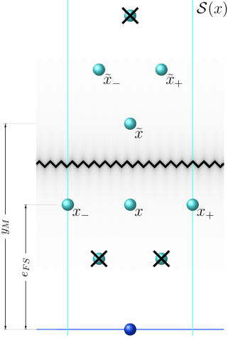
Figure 3. For models of types $\mathcal{M}^{0}_{\Lambda}(z)$ and $\mathcal{M}^{1}_{\Lambda}(z)$ with $x_{F}:=x_{F}^{0}$ the strip $\mathcal{S}(x)$ centered at a atom $x\in\partial\mathcal{L}_{FS}$ of a crystalline configuration $D_{n}$ is depicted as an example of a strip containing all the elements $x,x_{\pm},\tilde{x},\tilde{x}_{\pm}$ with the possibility of the strip center $x$ and the strip top $\tilde{x}$ to coincide if $y_{M}=e_{FS}$. The sites indicated by crossed atoms are sites of the planar lattice $\{x_{F}+k_{1}\bm{t}_{1}+k_{2}\bm{t}_{2}\,:\,\textrm{$k_{1},k_{2}\in\mathbb{Z}$}\}$ that surely are not in $D_{n}$ by definition of $\mathcal{L}_{F}$ and $\mathcal{S}(x)$.

In the following we refer to $x$ as the strip center of $\mathcal{S}(x)$, to $x_{\pm}$ as the strip lower (right and left) sides, to $\tilde{x}$ as the strip top, and to $\tilde{x}_{\pm}$ as the strip above (right and left) sides. Note that $x$ and $\tilde{x}$ coincide if $y_{M}=\color[rgb]{0,0,0}e_{FS}\color[rgb]{0,0,0}$.

We define the strip energy associated to a strip $\mathcal{S}(x)$ by

$$E_{\rm strip}(x):=E_{\rm strip,below}(x)\,+\,E_{\rm strip,above}({\color[rgb]{0,0,0}x}),$$ (27)

where

$$\\ E_{\rm strip,below}(x):=w(x)E_{\rm loc}(x)\,+\,w_{+}(x)E_{\rm loc}(x_{+})\,+\,w_{-}(x)E_{\rm loc}(x_{-})-c_{S},$$ (28)

with weights $w(x),w_{\pm}(x)\in\color[rgb]{0,0,0}\{1/4,1/2,1\}$ defined by

(29b)

(29c)

(29e)

and

$$E_{\rm strip,above}(x):=\begin{cases}E_{\rm loc}(\tilde{x})\,+\,\color[rgb]{0,0,0}w_{+}\color[rgb]{0,0,0}(\tilde{x})E_{\rm loc}(\tilde{x}_{+})\,+\,\color[rgb]{0,0,0}w_{-}\color[rgb]{0,0,0}(\tilde{x})E_{\rm loc}(\tilde{x}_{-})&\textrm{if $\tilde{x}\neq x$,}\\ \color[rgb]{0,0,0}w_{+}\color[rgb]{0,0,0}(\tilde{x})E_{\rm loc}(\tilde{x}_{+})\,+\,\color[rgb]{0,0,0}w_{-}\color[rgb]{0,0,0}(\tilde{x})E_{\rm loc}(\tilde{x}_{-}),&\textrm{if $\tilde{x}=x$}\end{cases}$$ (29ad)

with weights $w_{\pm}(\tilde{x})\in\color[rgb]{0,0,0}\{1/2,1\}$ given by

$$w_{\pm}(\tilde{x}):=\begin{cases}1&\textrm{if $x_{\pm}\not\in\color[rgb]{0,0,0}D_{n}\cap\partial\mathcal{L}_{FS}$ or \color[rgb]{0,0,0}$\tilde{x}_{\pm}\neq\widetilde{(x_{\pm})}_{\mp}$,}\\ \frac{1}{2}&\textrm{if $x_{\pm}\in\color[rgb]{0,0,0}D_{n}\cap\partial\mathcal{L}_{FS}$ and \color[rgb]{0,0,0}$\tilde{x}_{\pm}=\widetilde{(x_{\pm})}_{\mp}$}.\end{cases}$$ (29ae)

2.5. Almost-connected configurations

In this subsection we fix $x_{F}:=x_{F}^{0}$ and we introduce a weaker notion of connectedness of configurations valid for the models $\mathcal{M}^{0}_{\Lambda}(z)$ and $\mathcal{M}^{1}_{\Lambda}(z)$, which is needed to treat the situation when the wall parameter $q$ is not unitary, and so the energy is not invariant with respect to all horizontal translations of configurations. As we refer only to $\mathcal{M}^{0}_{\Lambda}(z)$ and $\mathcal{M}^{1}_{\Lambda}(z)$, we avoid in the section the dependence on the vectors $\Lambda\in(\mathbb{R}^{+})^{3}$ and $z\in Z_{S}$.

We recall from Section 2.1 that a configuration $D_{n}$ is said to be connected if every $x$ and $y$ in $D_{n}$ are connected through a path in the bonding graph of $D_{n}$, i.e., there exist $\ell\leq n$ and $x_{k}\in D_{n}$ for $k:=1,\dots,\ell$ such that $|x_{k}-x_{k-1}|=1$, $x_{1}=x$, and $x_{\ell}=y$, and we refer to maximal bonding subgraphs of $D_{n}$ connected through a path as connected components of $D_{n}$.

We say that a configuration $D_{n}$ is almost connected if it is connected when $q=1$, and, if there exists an enumeration of its $k:=k_{D_{n}}$ connected components, say $D_{n}^{i}$, $i=1,\dots,k$, such that each $D_{n}^{i}$ is separated by at most $q$ from $\cup_{l=1}^{i-1}D_{n}^{l}$ for every $i=2,\dots,n$, when $q\neq 1$. We say that a family of connected components of $D_{n}$ form an almost-connected component of $D_{n}$ if their union is almost connected and, if $q\neq 1$, it is distant from all other components of $D_{n}$ by more than $q$.

Definition 2.2.

Given a configuration $D_{n}\in\mathcal{C}_{n}$, we define the transformed configuration $\mathcal{T}(D_{n})\in\mathcal{C}_{n}$ of $D_{n}$ as

$$\mathcal{T}(D_{n}):=\mathcal{T}_{2}(\mathcal{T}_{1}(D_{n})),$$

where $\mathcal{T}_{1}(D_{n})$ is the configuration resulting by iterating the following procedure, starting from $D_{n}$:

• If there are connected components without any activated bond with an atom of $\partial\mathcal{L}_{S}$, then select one of those components with lowest distance from $\partial\mathcal{L}_{S}$;

• Translate the component selected at the previous step of a vector in direction $-\bm{t}_{2}$ till either a bond with another connected component or with the substrate is activated.

(notice that the procedure ends when all connected components of $\mathcal{T}_{1}(D_{n})$ have at least a bond with $\partial\mathcal{L}_{S}$), and $\mathcal{T}_{2}(\mathcal{T}_{1}(D_{n}))$ is the configuration resulting by iterating the following procedure, starting from $\mathcal{T}_{1}(D_{n})$:

• If there are more than one almost-connected component, then select the almost-connected component whose leftmost bond with $\partial\mathcal{L}_{S}$ is the second (when compared with the other almost-connected components) starting from the left;

• Translate the almost-connected component selected at the previous step of a vector $-kq\bm{t}_{1}$ for some $k\in\mathbf{N}$ till, if $q=1$, a bond with another connected component is activated, or, if $q\neq 1$, the distance with another almost-connected component is less or equal to $q$;

(notice that the procedure ends when $\mathcal{T}_{2}(D_{n})$ is almost connected).

We notice that the transformed configuration $\mathcal{T}(D_{n})$ of a configuration $D_{n}\in\mathcal{C}_{n}$ satisfies the following properties:

• $\mathcal{T}(D_{n})$ is almost connected;

• Each connected component of $\mathcal{T}(D_{n})$ includes at least an atom bonded to $\partial\mathcal{L}_{S}$;

• $V_{n}(\mathcal{T}(D_{n}))\leq V_{n}(D_{n})$ (as no active bond of $D_{n}$ is deactivated by performing the transformations $\mathcal{T}_{1}$ and $\mathcal{T}_{2}$);

and, if $D_{n}$ is a minimizer of $V_{n}$ in $\mathcal{C}_{n}$, then

• $\mathcal{T}_{1}(D_{n})\color[rgb]{0,0,0}=\color[rgb]{0,0,0}D_{n}$;

• $\mathcal{T}$ consists of translations of the almost-connected components of $D_{n}$ with respect to a vector (depending on the component) in the direction $-\bm{t}_{1}$ with norm in $\mathbb{N}\cup\{0\}$.

Finally we also observe that the definitions of $\mathcal{T}_{1}$, $\mathcal{T}_{2}$, and $\mathcal{T}$ are independent from $n$.

2.6. Continuum setting

We define the anisotropic surface tension $\Gamma:\mathbb{S}^{1}\to\mathbb{R}$ as the function for which

$$\Gamma(\nu(\varphi))=2c_{F}\left(\nu_{2}(\varphi)-\frac{\nu_{1}(\varphi)}{\sqrt{3}}\right)$$ (29af)

for every

$$\nu(\varphi)=\left(\begin{array}[]{c}-\sin\varphi\\ \cos\varphi\end{array}\right)\in\mathbb{S}^{1}\quad\text{with}\quad\varphi\in\left[0,\frac{\pi}{3}\right],$$

such that $\Gamma\circ\nu$ is extended periodically on $\mathbb{R}$ as a $\pi/3$-periodic function. Notice that $\color[rgb]{0,0,0}\Gamma(\pm\bm{t}_{3})=2c_{F}\color[rgb]{0,0,0}$ and that by extending $\Gamma$ by homogeneity we obtain a convex function, and in particular a Finsler norm on $\mathbb{R}^{2}$.

For every set of finite perimeter $D\subset\mathbb{R}^{2}\setminus S$ we formally define its anisotropic surface energy $\mathcal{E}$ by

$$\mathcal{E}_{\sigma}(D):=\int_{\color[rgb]{0,0,0}\partial^{*}D\backslash\partial S\color[rgb]{0,0,0}}\Gamma(\nu_{D})d\mathcal{H}^{1}+\sigma\mathcal{H}^{1}(\partial^{*}D\cap\partial S)$$ (29ai)

where $\partial^{*}D$ denotes the reduced boundary of $D$ and $\sigma\in\mathbb{R}$ is a parameter representing the adhesivity. Notice that in passing from the discrete to the continuum setting $\sigma$ will be characterized in terms of the parameters of the discrete settings with conditions in particular entailing the lower semicontinuity of $\mathcal{E}_{\sigma}$.

2.7. Main results

In this section the main theorems proven in the manuscript are stated. Let us classify all the models $\mathcal{M}_{\Lambda}(x_{F},z)$ of type (18) for interaction vectors $\Lambda:=(e_{FS},c_{F},c_{S})\in(\mathbb{R}^{+})^{3}$, film-lattice centers $x_{F}\in\mathbb{R}^{2}\setminus\overline{S}$, and wall vectors $z\in Z_{S}^{0}$ such that (13) holds (see Figure 4), in four categories, namely by saying that $\mathcal{M}_{\Lambda}(x_{F},z)\in C_{i}$ with the classes of models $C_{i}:=C_{i}(\Lambda,x_{F},z)$ given for $i=1,\dots,4$ by:

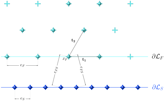
Figure 4. Example of a model $\mathcal{M}_{\Lambda}(x_{F},z)$ of type (18) with wall vectors $z=(2,1,0)\in Z_{S}^{0}$, which is in particular in the class $C_{1}$.

• models with $x_{F}$ having two substrate neighbors;

• models with $x_{F}$ having exactly one substrate neighbor and

  $$(x_{F},x_{F}+q\bm{t}_{1})\cap\partial\mathcal{L}_{FS}(x_{F},z)=\emptyset;$$

• models with $x_{F}$ having exactly one substrate neighbor and

  $$(x_{F},x_{F}+q\bm{t}_{1})\cap\partial\mathcal{L}_{FS}(x_{F},z)=\{x_{F}+\frac{q}{2}\bm{t}_{1}\}$$

  (which implies that $q$ is even);

• model with $x_{F}$ having exactly one substrate neighbor, $q>2$, and for which there exists $s\in\{1,\dots,q-1\}\setminus\{q/2\}$ such that

  $$(x_{F},x_{F}+q\bm{t}_{1})\cap\partial\mathcal{L}_{FS}(x_{F},z)=\{x_{F}+s\bm{t}_{1}\}.$$

Notice that by the proof of Proposition 4.1 in particular follows that for every model $\mathcal{M}_{\Lambda}(x_{F},z)$ with $z\in Z_{S}^{0}$ there exists a unique $i_{0}\in\{1,\dots,4\}$ such that $\mathcal{M}_{\Lambda}(x_{F},z)\in C_{i_{0}}$, and that any model $\mathcal{M}_{\Lambda}(x_{F},z)\in C_{i}$ for $i\in\{1,\dots,4\}$ is such that $\partial\mathcal{L}_{FS}:=\{x_{F}+k:k\in L_{i}\}$ with

$$L_{i}:=\begin{cases}q\mathbb{Z}&\text{if $i=1,2$,}\\ \frac{q}{2}\mathbb{Z}&\text{if $i=3$,}\\ q\mathbb{Z}\cup(q\mathbb{Z}+s)&\text{if $i=4$.}\\ \end{cases}$$

We begin with the following result that characterizes the wetting regime in terms of a condition only depending on $v_{FF}$ and $v_{FS}$, and the minimizers in such regime, which we denote as wetting configurations. More precisely, we say that a configuration $D^{\rm w}_{n}:=\{w_{1},\dots,w_{n}\}\in\mathcal{C}_{n}(x_{F})$ is a wetting configuration

• if $D^{\rm w}_{n}\subset\partial\mathcal{L}_{FS}(x_{F},z)$ when either $\mathcal{M}_{\Lambda}(x_{F},z)\in C_{i}$ for $i=1,2$ and $q>1$, or $\mathcal{M}_{\Lambda}(x_{F},z)\in C_{3}$ and $q>2$, or $\mathcal{M}_{\Lambda}(x_{F},z)\in C_{4}$ and $1<s<q-1$;

• if $D^{\rm w}_{n}\subset\partial\mathcal{L}_{FS}(x_{F},z)$ and

  $$w_{i+1}:=w_{i}+\bm{t}_{1}$$ (29aj)

  for every $i=1,\dots,{n}$, when either $\mathcal{M}_{\Lambda}(x_{F},z)\in C_{i}$ for $i=1,2$ and $q=1$ or $\mathcal{M}_{\Lambda}(x_{F},z)\in C_{3}$ and $q=2$;

• if $D^{\rm w}_{n}\subset\partial\mathcal{L}_{FS}(x_{F},z)$ and for every $i=1,\dots,{n}$ up to one index in the case $n$ is odd we have that either $w_{i}+\bm{t}_{1}$ or $w_{i}-\bm{t}_{1}$ belongs to $D^{\rm w}_{n}$ as well, when $\mathcal{M}_{\Lambda}(x_{F},z)\in C_{4}$ and $s=1$ or $s=q-1$.

Theorem 2.3 (Wetting regime).

For every $n\in\mathbb{N}$ any wetting configuration $D^{\rm w}_{n}\in\mathcal{C}_{n}(x_{F})$ satisfies the following two assertions:

• $V_{n}(D^{\rm w}_{n})=\min{V_{n}(D_{n})}$,

• $V_{n}(D^{\rm w}_{n})<V_{n}(D_{n})$ for every crystalline configuration $D_{n}\in\mathcal{C}_{n}(x_{F})$ that is not a wetting configuration,

if and only if

$$\begin{cases}c_{S}\geq 6c_{F}&\text{if either $\mathcal{M}_{\Lambda}(x_{F},z)\in C_{i}$ for $i=1,2$ and $q>1$, or $\mathcal{M}_{\Lambda}(x_{F},z)\in C_{3}$}\\ &\text{and $q>2$, or $\mathcal{M}_{\Lambda}(x_{F},z)\in C_{4}$ and $1<s<q-1$},\\ c_{S}\geq 5c_{F}&\text{if $\mathcal{M}_{\Lambda}(x_{F},z)\in C_{4}$ and $s=1$ or $s=q-1$},\\ c_{S}\geq 4c_{F}&\text{if either $\mathcal{M}_{\Lambda}(x_{F},z)\in C_{i}$ for $i=1,2$ and $q=1$, or $\mathcal{M}_{\Lambda}(x_{F},z)\in C_{3}$}\\ &\text{and $q=2$}.\end{cases}$$ (29ak)

In particular, for the necessity of (29ax) it is enough assertion (i), and more specifically that there exists an increasing subsequence $(n_{k})_{k\in\mathbf{N}}$ such that $V_{n_{k}}(D^{\rm w}_{n_{k}})=\min{V_{n_{k}}(D_{n_{k}})}$ holds for every $n_{k}$.

We refer to (29ax) as a wetting condition or as the wetting regime, and to the opposite condition, namely

$$\begin{cases}c_{S}<6c_{F}&\text{if either $\mathcal{M}_{\Lambda}(x_{F},z)\in C_{i}$ for $i=1,2$ and $q>1$, or $\mathcal{M}_{\Lambda}(x_{F},z)\in C_{3}$}\\ &\text{and $q>2$, or $\mathcal{M}_{\Lambda}(x_{F},z)\in C_{4}$ and $1<s<q-1$},\\ c_{S}<5c_{F}&\text{if $\mathcal{M}_{\Lambda}(x_{F},z)\in C_{4}$ and $s=1$ or $s=q-1$},\\ c_{S}<4c_{F}&\text{if either $\mathcal{M}_{\Lambda}(x_{F},z)\in C_{i}$ for $i=1,2$ and $q=1$, or $\mathcal{M}_{\Lambda}(x_{F},z)\in C_{3}$}\\ &\text{and $q=2$,}\end{cases}$$ (29al)

as the dewetting condition or the dewetting regime. The following result shows that connected components with the largest cardinality of minimizers incorporate the whole mass in the limit.

Theorem 2.4 (Mass conservation).

Assume (29al). If $\widehat{D}_{n}$ are minimizers of $V_{n,\Lambda}$ among all crystalline configurations in $\mathcal{C}_{n}$, i.e.,

$$V_{n,\Lambda}(\widehat{D}_{n})=\min_{D_{n}\in\mathcal{C}_{n}}{V_{n,\Lambda}(D_{n})},$$

and we select for every $\widehat{D}_{n}$ a connected component $\widehat{D}_{n,1}\subset\widehat{D}_{n}$ with largest cardinality, then

$$\lim_{n\to\infty}{\mu_{\widehat{D}_{n}}(\widehat{D}_{n,1})}=1,$$

where $\mu_{\widehat{D}_{n}}$ are the empirical measure associated to $\widehat{D}_{n}$ defined by (20).

We rigorously prove by $\Gamma$-convergence that the discrete models converge to the continuum model, and in view of the previous result (even in the lack of a direct compactness result for general sequences of minimizers, possibly not almost connected), we prove convergence (up to passing to a subsequence and up to translations) of the minimizers of the discrete models to a bounded minimizer of the continuum model, which in turn is also proven to exist.

Theorem 2.5 (Convergence of Minimizers).

Assume (29al). The following statements hold:

• The functional

  $$E_{n,\Lambda,x_{F}}:=n^{-1/2}(I_{n,\Lambda,x_{F}}+6c_{F}n),$$ (29am)

  where $I_{n,\Lambda,x_{F}}$ is defined by (LABEL:radon_functional), $\Gamma$-converges with respect to the weak* convergence of measures to the functional $I_{\infty,i}$ defined by

  $$\hskip 14.22636ptI_{\infty,i}(\mu):=\begin{cases}\mathcal{E}_{\sigma_{i}}(D_{\mu}),&\text{if \color[rgb]{0,0,0}there exists \color[rgb]{0,0,0}$D_{\mu}\subset\mathbb{R}^{2}\setminus S$ set of finite perimeter}\\ &\text{with $|D_{\mu}|=1/\rho$ such that $\mu=\rho\chi_{D_{\mu}}$,}\\ +\infty,&\text{otherwise,}\\ \end{cases}$$ (29an)

  for every $\mu\in\mathcal{M}(\mathbb{R}^{2})$, where $\rho:=2/\sqrt{3}$ and $\mathcal{E}_{\sigma_{i}}$ is defined in (29ai) for an adhesivity $\sigma:=\sigma_{i}$ given for $i=1,\dots,4$ by

  $$\sigma_{i}:=\begin{cases}2c_{F}-\displaystyle\frac{2c_{S}}{q}&\text{if $i=1,3,4$ and $\mathcal{M}_{\Lambda}(x_{F},z)\in C_{i}$,}\\ &\\ 2c_{F}-\displaystyle\frac{c_{S}}{q}&\text{if $i=2$ and $\mathcal{M}_{\Lambda}(x_{F},z)\in C_{2}$.}\\ \end{cases}$$ (29ao)

• The functional $I_{\infty,i}$ admits a minimizer in

  $$\mathcal{M}_{W}:=\bigg{\{}\mu\in\mathcal{M}(\mathbb{R}^{2})\ :\ \text{$\exists$ $D\subset\mathbb{R}^{2}\setminus S$}$$ set of finite perimeter, bounded

  $$\hskip 34.44434pt\text{with }|D|=\frac{1}{\rho}, \hskip 8.61108pt\text{ and such that $\mu=\rho\chi_{D}$}\bigg{\}}.$$ (29ap)

• Every sequence $\mu_{n}\in\mathcal{M}_{n}(x_{F})$ of minimizers of $E_{n,\Lambda,x_{F}}$ admits, up to translation a subsequence converging with respect to the weak* convergence of measures to a minimizer of $I_{\infty,i}$ in $\mathcal{M}_{W}$.

Notice that the parameter $\rho:=2/\sqrt{3}$ in the definition of $\mathcal{M}_{W}$ is related to the fact that we chose the triangular lattice for $\mathcal{L}_{F}(x_{F})$, as $\rho$ is the density of atoms per unit volume of such lattice.

Finally, we observe that as a byproduct of our strategy analogous results as Theorems 2.3, 2.4, and 2.5 are also obtained for any models $\mathcal{M}^{1}_{\Lambda}(z)$ with $z\in Z^{1}_{S}$ and $\Lambda\in(\mathbb{R}^{+})^{3}$, namely in Theorems 3.4, 3.9, and 3.10, respectively.

3. Model $\mathcal{M}^{1}_{\Lambda}(z)$

In this section we prove analogous results of the ones contained in Section 2.7 for the specific model $\mathcal{M}^{1}_{\Lambda}(z)$ defined in Section 2.2 for $z\in Z_{S}^{1}$ and $\Lambda:=(e_{FS},c_{F},c_{S})\in(\mathbb{R}^{+})^{3}$, i.e., Theorems 3.4, 3.9, and 3.10, respectively. In this section for simplicity we often avoid indicating the dependence on $x_{F}:=x_{F}^{0}$ and on $\Lambda\in(\mathbb{R}^{+})^{3}$ as we only deal with models $\mathcal{M}^{1}_{\Lambda}(z)$.

We start by characterizing the wetting regime for the model $\mathcal{M}^{1}_{\Lambda}(z)$. In the following we say that a configuration $D^{\rm w}_{n}:=\{w_{1},\dots,w_{n}\}\in\mathcal{C}_{n}$ is a wetting configuration for $\mathcal{M}^{1}_{\Lambda}(z)$ if:

• $D^{\rm w}_{n}\subset\partial\mathcal{L}_{FS}(z)$ for $z\in Z_{S}^{1}$ with $r>1$ (and so $q>2$);

• $D^{\rm w}_{n}:=\{w_{1},\dots,w_{n}\}\subset\partial\mathcal{L}_{FS}(z)$ with

  $$w_{i+1}:=w_{i}+\bm{t}_{1}$$ (29aq)

  for every $i=1,\dots,{n}$, for $z\in Z_{S}^{1}$ with $r=1$ and $q=2$;

• $D^{\rm w}_{n}:=\{w_{1},\dots,w_{n}\}\in\mathcal{L}_{FS}(z)$ such that for every $i=1,\dots,{n}$ up to one index in the case $n$ is odd we have that either $w_{i}+\bm{t}_{1}$ or $w_{i}-\bm{t}_{1}$ belongs to $D^{\rm w}_{n}$ as well, for $z\in Z_{S}^{1}$ with $r=1$ and $q>2$.

Proposition 3.1.

Let $n\in\mathbb{N}$ and $z\in Z_{S}^{1}$ with $r>1$ (and so $q>2$). Any wetting configuration $D^{\rm w}_{n}\subset\partial\mathcal{L}_{FS}(z)$ satisfies the following two assertions:

• $V_{n}(D^{\rm w}_{n})=\min{V_{n}(D_{n})}$,

• $V_{n}(D^{\rm w}_{n})<V_{n}(D_{n})$ for any $D_{n}$ that is not a wetting configuration,

if and only if

$$c_{S}\geq 6c_{F}.$$ (29ar)

Proof.

The proof is the same as the proof of Proposition 3.1 in [25] for the model $\mathcal{M}^{0}$ with $q\neq 1$, by observing that

$$V_{n}(D^{\rm w}_{n})=-c_{S}n.$$ (29as)

also with respect to the model $\mathcal{M}^{1}_{\Lambda}(z)$ for the conditions of the assertion on the wall parameters.

∎

We now consider the case of $z\in Z_{S}^{1}$ with $r=1$ and $q=2$ (for which $\mathcal{M}^{1}_{\Lambda}(q,r)=\mathcal{M}^{0}_{\Lambda}(1,q/2)$ as observed in Section 2.2) where it is possible for connected configurations to have all atoms bonded with a substrate atom.

Proposition 3.2.

Let $n\in\mathbb{N}$ and $z\in Z_{S}^{1}$ with $r=1$ and $q=2$. Any wetting configuration $D^{\rm w}_{n}\subset\partial\mathcal{L}_{FS}(z)$ satisfies the following two assertions:

• $V_{n}(D^{\rm w}_{n})=\min{V_{n}(D_{n})}$,

• $V_{n}(D^{\rm w}_{n})<V_{n}(D_{n})$ for any $D_{n}$ that is not a wetting configuration,

if and only if

$$c_{S}\geq 4c_{F}.$$ (29at)

Proof.

The proof is the same as the proof of Proposition 3.2 in [25] for the model $\mathcal{M}^{0}$ with $q=1$, by observing that

$$V_{n}(D^{\rm w}_{n})=-c_{S}n-2c_{F}(n-1)$$ (29au)

also with respect to the model $\mathcal{M}^{1}_{\Lambda}(z)$ for the conditions of the assertion on the wall parameters.

∎

We finally address the remaining case of $r=1$ and $q>2$ for which we notice that $\partial\mathcal{L}_{FS}$ contains separated pairs of neighboring film atoms.

Proposition 3.3.

Let $n\in\mathbb{N}$ and $z\in Z_{S}^{1}$ with $r=1$ and $q>2$. Any wetting configuration $D^{\rm w}_{n}\subset\partial\mathcal{L}_{FS}(z)$ satisfies the following two assertions:

• $V_{n}(D^{\rm w}_{n})=\min{V_{n}(D_{n})}$,

• $V_{n}(D^{\rm w}_{n})<V_{n}(D_{n})$ for any $D_{n}$ that is not a wetting configuration,

if and only if

$$c_{S}\geq 5c_{F}.$$ (29av)

Proof.

The proof is based on the same arguments employed for previous two propositions and on the following observations. Note that (i) easily follows from (ii) and the fact that any wetting configuration $D^{\rm w}_{n}$ for $r=1$ and $q>2$ has the same energy given by

$$V_{n}(D^{\rm w}_{n})=-c_{S}n-c_{F}(n-1).$$ (29aw)

if $n$ is odd, and

$$V_{n}(D^{\rm w}_{n})=-c_{S}n-c_{F}n.$$

if $n$ is even.

For the sufficiency of (29av) in order to prove (ii) we proceed by induction on $n$. We first notice that (ii) is trivial for $n=1$. Then, we assume that (ii) holds true for every $k=1,\dots,n-1$ and prove that it holds also for $n$. Let $D_{n}$ be a crystalline configuration that is not a wetting configuration for $r=1$ and $q>2$. We can assume without loss of generality that $D_{n}\cap(\mathbb{R}\times\{s>e_{S}\})\neq\emptyset$ because if not, we can easily see that the energy of $D_{n}$ is higher than the energy of $D^{\rm w}_{n}$ at least by $c_{S}-2c_{F}$, which is positive by (29av), since the elements in $D_{n}\setminus\partial\mathcal{L}_{FS}\neq\emptyset$ have at most two film bonds and no substrate bonds. Let $L$ be the last line in $\mathbb{R}\times\{s>0\}$ parallel to $\bm{t}_{1}$ that intersects $D_{n}$ by moving upwards from $\mathbb{R}\times\{e_{S}\}$ (which exists since $D_{n}$ has a finite number of atoms). We can then use the same argument used for [25, Eq. (36)] to prove that

$$V_{n}(D_{n}) \geq V_{n-\ell}(D_{n}\backslash L)-6c_{F}(\ell-1)-4c_{F}$$

and hence, by induction hypothesis if $n$ is odd (the other case being analogous), we have that

$$V_{n}(D_{n}) \geq V_{n-\ell}(D_{n}\backslash L)-6c_{F}(\ell-1)-4c_{F}>V_{n-\ell}(D_{n}\backslash L)-6c_{F}\ell$$

$$>-c_{S}(n-\ell)-c_{F}(n-\ell-1)-6c_{F}\ell\geq-c_{S}n$$

$$>-c_{S}(n-\ell)-(c_{F}(n-\ell-1)+c_{F}\ell)-5c_{F}\ell$$

$$\geq-c_{S}n-c_{F}(n-1)=V_{n}(D^{\rm w}_{n}),$$

where we used (29av) in the last inequality and (29aw) in the last equality.

In order to prove the necessity of (29av) for assertions (i) and (ii), we consider the Wulff shape with $n$ atoms in $\mathbb{R}\times\{s>\color[rgb]{0,0,0}e_{FS}\color[rgb]{0,0,0}\}$ which has energy $-6c_{F}n+C\sqrt{n}$ for some constant $C>0$, and observe that

$$-c_{S}n-c_{F}n<-6c_{F}n+C\sqrt{n}$$

by assertion (ii). From dividing by $n$ and letting $n\to\infty$ we obtain (29av).

∎

We are now ready to characterize the wetting regime for the models $\mathcal{M}^{1}_{\Lambda}(z)$. We refer to (29ar), (29at) and (29av) as wetting conditions.

Theorem 3.4 (Wetting regime for $\mathcal{M}^{1}_{\Lambda}(z)$).

For every $n\in\mathbb{N}$ any wetting configuration $D^{\rm w}_{n}\in\mathcal{C}_{n}$ satisfies the following two assertions:

• $V_{n}(D^{\rm w}_{n})=\min{V_{n}(D_{n})}$,

• $V_{n}(D^{\rm w}_{n})<V_{n}(D_{n})$ for every crystalline configuration $D_{n}\in\mathcal{C}_{n}$ that is not a wetting configuration,

if and only if

$$\begin{cases}c_{S}\geq 6c_{F}&\text{if $z\in Z_{S}^{1}$ with $r>1$ \emph{(}and so $q>2$\emph{)},}\\ c_{S}\geq 5c_{F}&\text{if $z\in Z_{S}^{1}$ with $r=1$ and $q>2$},\\ c_{S}\geq 4c_{F}&\text{if $z\in Z_{S}^{1}$ with $r=1$ and $q=2$}.\end{cases}$$ (29ax)

In particular, for the necessity of (29ax) it is enough assertion (i), and more specifically that there exists an increasing subsequence $(n_{k})_{k\in\mathbf{N}}$ such that $V_{n_{k}}(D^{\rm w}_{n_{k}})=\min{V_{n_{k}}(D_{n_{k}})}$ holds for every $n_{k}$.

Proof.

The first assertion directly follows from Propositions 3.1, 3.2, and 3.3 for $z\in Z^{1}_{S}$, while the second assertion is a direct consequence of the limiting procedure in the proofs of the necessity of the wetting conditions of such results.

∎

We now move on studying the dewetting regime for the model $\mathcal{M}^{1}_{\Lambda}(z)$. Therefore, in the remaining part of this section we work only under the assumption

$$\begin{cases}c_{S}<6c_{F}&\text{if $z\in Z_{S}^{1}$ with $r>1$ (and so $q>2$),}\\ c_{S}<5c_{F}&\text{if $z\in Z_{S}^{1}$ with $r=1$ and $q>2$},\\ c_{S}<4c_{F}&\text{if $z\in Z_{S}^{1}$ with $r=1$ and $q=2$}.\end{cases}$$ (29ay)

We begin by establishing a lower bound uniform for every $x\in D_{n}\cap\partial\mathcal{L}_{FS}$ in terms of $c_{F}$ and $c_{S}$ of the strip energy $E_{\rm strip}(x)$ defined in Section 2.4.

Lemma 3.5.

If (29ay) holds, then

$$E_{\rm strip}(x)\geq\Delta_{\rm strip}$$

with

$$\Delta_{\rm strip}:=\begin{cases}6c_{F}-c_{S}&\text{if $z\in Z_{S}^{1}$ with $r>1$ \emph{(}and so $q>2$\emph{)},}\\ 5c_{F}-c_{S}&\text{if $z\in Z_{S}^{1}$ with $r=1$ and $q>2$},\\ 4c_{F}-c_{S}&\text{if $z\in Z_{S}^{1}$ with $r=1$ and $q=2$},\end{cases}$$ (29az)

for every $x\in D_{n}\cap\partial\mathcal{L}_{FS}$.

Proof.

Fix $x\in D_{n}\cap\partial\mathcal{L}_{FS}$. We begin by observing that the strip center $x$ surely misses the bonds with the atoms missing at the 2 positions $x-\bm{t}_{2}+k\bm{t}_{1}$ for $k=0,1$ as shown in Figure 3. Furthermore, either $x$ misses the bond with $x_{-}$, or $x_{-}\in{\color[rgb]{0,0,0}D_{n}}$ and $x_{-}$ misses the bonds with the 2 positions $x-\bm{t}_{2}+k\bm{t}_{1}$ for $k=-1,0$ (which in the strip energy are counted with half weights). We can reason similarly for $x_{+}$. Therefore, by the definition of energy of the low strip $E_{\rm strip,below}$, we obtain that

$$E_{\rm strip,below}\color[rgb]{0,0,0}\geq\color[rgb]{0,0,0}\begin{cases}4c_{F}-c_{S}&\text{if $z\in Z_{S}^{1}$ with $r>1$ (and so $q>2$),}\\ 3c_{F}-c_{S}&\text{if $z\in Z_{S}^{1}$ with $r=1$ and $q>2$},\\ 2c_{F}-c_{S}&\text{if $z\in Z_{S}^{1}$ with $r=1$ and $q=2$}.\end{cases}$$

The analysis of $E_{strip,above}$ is exactly the same as in [25, Lemma 4.1] since $E_{strip,above}$ for $\mathcal{M}^{1}z$ for $z\in Z_{S}^{1}$ is defined as for $\mathcal{M}^{0}$. In particular, the terms related to the triple $\tilde{x}$, $\tilde{x}_{+}$, and $\tilde{x}_{-}$ give always a contribution in the strip energy $E_{\rm strip}$ of at least $2c_{F}$.

∎

In the following result by employing a similar non-local strip argument of [25, Lemma 4.2] related to the more involved definition of the strip $\mathcal{S}$ of Section 2.4 we can show that the energy $V_{n}(D_{n})$ of any crystalline configuration $D_{n}$ is bounded from below by $-6c_{F}n$ plus a positive deficit due to the contribution of the boundary of $D_{n}$, i.e., where atoms have less than 6 film bonds and could have a bond with the substrate.

Lemma 3.6.

If (29ay) holds, then there exists $\Delta>0$ such that

$$V_{n}(D_{n})\geq-6c_{F}n\,+\,\Delta\#\partial D_{n}$$ (29ba)

for every crystalline configuration $D_{n}\subset\mathcal{L}_{F}$. Furthermore, the following two assertions are equivalent:

• There exists a constant $C>0$ such that $\#\partial D_{n}\leq C\sqrt{n}$ for every $n\in\mathbb{N}$,

• There exists a constant $C^{\prime}>0$ such that $E_{n}(\mu_{D_{n}})\leq C^{\prime}$ for every $n\in\mathbb{N}$.

Proof.

The proof is analogous to the proof of [25, Lemma 4.2] where instead of [25, Lemma 4.1] we apply Lemma 3.5. In fact, by (24) and (27) we observe that also by the careful choice of the weights (29b)-(29c) in (28), besides of the choice of weights (29ae) in (29ad), we have that

$$6c_{F}n\,+\,V_{n}(D_{n})\, =\,\sum_{x\in D_{n}}\left(\sum_{y\in{\color[rgb]{0,0,0}D_{n}}\setminus\{x\}}v_{FF}(|x-y|)+6c_{F}\right)\,+\,\sum_{x\in D_{n}}v^{1}(x)$$

$$=\,\sum_{x\in D_{n}}E_{\rm loc}(x)\,+\,\sum_{x\in D_{n}}v^{1}(x)$$

$$\geq\,\sum_{x\in D_{n}\cap{\color[rgb]{0,0,0}\partial\mathcal{L}_{FS}}}E_{\rm strip}(x)\,+\,\sum_{x\in D_{n}\setminus\mathcal{S}({\color[rgb]{0,0,0}\partial\mathcal{L}_{FS}})}E_{\rm loc}(x).$$ (29bb)

with

$$\mathcal{S}(\partial\mathcal{L}_{FS})=\mathcal{S}_{\color[rgb]{0,0,0}D_{n}\color[rgb]{0,0,0}}({\color[rgb]{0,0,0}\partial\mathcal{L}_{FS}}):=\{y\in\mathcal{S}(x)\,:\,x\in D_{n}\cap{\color[rgb]{0,0,0}\partial\mathcal{L}_{FS}}\},$$ (29bc)

where we used that $v^{1}(x)=0$ for every $x\in D_{n}\setminus\partial\mathcal{L}_{FS}$, since the local energy $E_{\rm loc}(x)$ of every film atom in $D_{n}\cap{\color[rgb]{0,0,0}\partial\mathcal{L}_{FS}}$ is counted at most once.

∎

In view of the previous lower bound for the energy of a configuration $D_{n}$ we are able to compensate the negative contribution coming at the boundary from the interaction with the substrate obtaining the following compactness results.

Proposition 3.7.

Assume that (29ay) holds. Let $D_{n}\in\mathcal{C}_{n}$ be almost-connected configurations such that

$$V_{n}(D_{n})\leq-6c_{F}n+Cn^{1/2}$$ (29bd)

for a constant $C>0$. Then there exist an increasing sequence $n_{r}$, $r\in\mathbb{N}$, and a measure $\mu\in\mathcal{M}(\mathbb{R}^{2})$ with $\mu\geq 0$ and $\mu(\mathbb{R}^{2})=1$ such that $\mu_{r}\stackrel{{\scriptstyle*}}{{\rightharpoonup}}\mu$ in $\mathcal{M}(\mathbb{R}^{2})$, where $\mu_{r}:=\mu_{D_{n_{r}}\color[rgb]{0,0,0}(\,\cdot\,+a_{n_{r}})}$ for some translations $a_{n}\in\mathbb{R}^{2}$ (see (20) for the definition of the empirical measures $\mu_{D_{n_{r}}}$). Moreover, if $D_{n}\in\mathcal{C}_{n}$ are minimizers of $V_{n}$ in $\mathcal{C}_{n}$, then we can choose $a_{n}=t_{n}\bm{t}_{1}$ for integers $t_{n}\in\mathbb{Z}$.

Proof.

The proof follows the same strategies employed for the proof of [25, Proposition 4.3], where instead of applying [25, Lemma 4.2] we apply the previously proven Lemma 3.6. ∎

We are now ready to state the following compactness result which is a consequence of Proposition 3.7 and of the definition of transformed configuration $\mathcal{T}(D_{n})$ associated to a configuration $D_{n}$ provided in Definition 2.2 (see also (see also [25, Theorem 4.1] and [2, Theorem 1.1]).

Theorem 3.8 (Compactness).

Assume that (29ay) holds. Let $D_{n}\in\mathcal{C}_{n}$ be configurations satisfying (29bd) and let $\mu_{n}:=\mu_{\mathcal{T}(D_{n})}$ be the empirical measures associated to the transformed configurations $\mathcal{T}(D_{n})\in\mathcal{C}_{n}$ associated to $D_{n}$ by Definition 2.2. Then, up to translations $($i.e., up to replacing $\mu_{n}$ by $\mu_{n}(\cdot+a_{n})$ for some $a_{n}\in\mathbb{R}^{2}$$)$ and a passage to a non-relabelled subsequence, $\mu_{n}$ converges weakly* in $\mathcal{M}(\mathbb{R}^{2})$ to a measure $\mu\in\mathcal{M}_{W}$, where $\mathcal{M}_{W}$ is defined in (29bh). Furthermore, if $D_{n}\in\mathcal{C}_{n}$ are minimizers of $V_{n}$ in $\mathcal{C}_{n}$, then we can choose $a_{n}=t_{n}\bm{t}_{1}$ for integers $t_{n}\in\mathbb{Z}$.

The next results allows to overcome the issue of compactness for not almost-connected configurations (without using associated transformed configurations as in Theorem 3.8), as it shows that mass is preserved in the limit by carefully selecting connected components of minimizers.

Theorem 3.9 (Mass conservation).

Assume that (29ay) holds. If $\widehat{D}_{n}$ are minimizers of $V_{n,\Lambda}$ among all crystalline configurations in $\mathcal{C}_{n}$, i.e.,

$$V_{n,\Lambda}(\widehat{D}_{n})=\min_{D_{n}\in\mathcal{C}_{n}}{V_{n,\Lambda}(D_{n})},$$

and we select for every $\widehat{D}_{n}$ a connected component $\widehat{D}_{n,1}\subset\widehat{D}_{n}$ with largest cardinality, then

$$\lim_{n\to\infty}{\mu_{\widehat{D}_{n}}(\widehat{D}_{n,1})}=1,$$

where $\mu_{\widehat{D}_{n}}$ are the empirical measure associated to $\widehat{D}_{n}$ defined by (20).

The proof of Theorem 3.9 is exactly the same as for the analogous [25, Theorem 2.3] and it actually depends on the first two assertions of the following theorem (whose statement we postpone below as it requires some adjustment in the proof): first one establishes the $\Gamma$-convergence result (see Assertion 1 of Theorem 3.10), which together with Theorem 3.8 implies the existence of minimizer (see Assertion 2 of Theorem 3.10) for the limiting functional $I_{\infty,4}$ defined in (29bf), then, one shows that it is impossible for a sequence of minimizers of $E_{n,\Lambda,x_{F}}$ to have a subsequence of disconnected components with significant mass, since this would imply that there exists a disconnected minimizer of $I_{\infty,4}$, which it is an absurd by scaling arguments.

Theorem 3.10 (Convergence of Minimizers).

Assume that (29ay) holds. The following statements hold:

• The functional

  $$E_{n,\Lambda,x_{F}}:=n^{-1/2}(I_{n,\Lambda,x_{F}}+6c_{F}n),$$ (29be)

  where $I_{n,\Lambda,x_{F}}$ is defined by (LABEL:radon_functional), $\Gamma$-converges with respect to the weak* convergence of measures to the functional $I_{\infty,4}$ defined by

  $$I_{\infty,4}(\mu):=\begin{cases}\mathcal{E}_{\sigma_{4}}(D_{\mu}),&\text{if \color[rgb]{0,0,0}there exists \color[rgb]{0,0,0}$D_{\mu}\subset\mathbb{R}^{2}\setminus S$ set of finite perimeter}\\ &\hskip 64.58313pt\text{with $|D_{\mu}|=1/\rho$ such that $\mu=\rho\chi_{D_{\mu}}$,}\\ +\infty,&\text{otherwise,}\\ \end{cases}$$ (29bf)

  for every $\mu\in\mathcal{M}(\mathbb{R}^{2})$, where $\rho:=2/\sqrt{3}$ and $\mathcal{E}_{\sigma_{4}}$ is defined in (29ai) for an adhesivity $\sigma:=\sigma_{4}$ where

  $$\sigma_{4}:=2c_{F}-\displaystyle\frac{2c_{S}}{q}.$$ (29bg)

• The functional $I_{\infty,4}$ admits a minimizer in

  $$\mathcal{M}_{W}:=\bigg{\{}\mu\in\mathcal{M}(\mathbb{R}^{2})\ :\ \text{$\exists$ $D\subset\mathbb{R}^{2}\setminus S$}$$ set of finite perimeter, bounded

  $$\hskip 34.44434pt\text{with }|D|=\frac{1}{\rho}, \hskip 8.61108pt\text{ and such that $\mu=\rho\chi_{D}$}\bigg{\}}.$$ (29bh)

• Every sequence $\mu_{n}\in\mathcal{M}_{n}$ of minimizers of $E_{n,\Lambda,x_{F}}$ admits, up to translation a subsequence converging with respect to the weak* convergence of measures to a minimizer of $I_{\infty,4}$ in $\mathcal{M}_{W}$.

To prove Theorem 3.10 we follow the proof of [25, Theorem 2.4], which consists in proving the lower and the upper bound established in [25, Theorems 5.3 and 6.1], respectively. The upper bound can be proven in the exact same way as done in [25, Theorem 6.1]: the set $D\subset\mathbb{R}^{2}\backslash S$ of finite perimeter satisfying $|D|=1/\rho$ is approximated first by smooth bounded sets, then by polygons, then by polygons with vertices on the lattice, and finally by the sequence of configurations $(D_{n})_{n\in\mathbb{N}}$ such that $D_{n}\in\mathcal{C}_{n}$, $\mu_{D_{n}}\stackrel{{\scriptstyle*}}{{\rightharpoonup}}\rho\chi_{D}$ and $I_{n,\Lambda,x_{F}}(\mu_{D_{n}})\to I_{\infty,4}(\rho\chi_{D})$.

The lower bound can be proven by an adaptation of the arguments of the proof of [25, Theorem 5.3]. We first describe the overall strategy and then highlight the main differences in such arguments in the proof below.

The strategy consists in associating to each configuration $D_{n}$ an auxiliary set $H_{n}^{\prime}$ such that $\chi_{H_{n}^{\prime}}$ converges in $BV_{\rm loc}$ to $\chi_{D}$ (see also [2]) in order to transfer the problem on the surface energy functionals analyzed in, e.g., [3]. Furthermore, by fixing $\delta>0$ we reduce the analysis to the region $\{x\in\mathbb{R}^{2}:0\leq x_{2}\leq\delta\}$, since outside of it one can simply use Reshetnyak Lower-Semiconinuity Theorem. For the points $x\in\partial^{*}D\cap\{x_{2}=0\}$ one obtains the lower bound by using the fact that for $n$ large enough the upper half of an arbitrary small square with center in $x$ and sides parallel to the coordinate axes is “approximately filled” by the set $H_{n}^{\prime}$ and hence, containing in the worst case all the atoms that have substrate neighbors, whose energy density is $-2c_{S}/q$. However, also the other atoms without substrate neighbors must be contained, and every boundary atom in such upper half of the arbitrary small square on every line perpendicular to $x_{2}=0$ brings the energy density of $2c_{F}$. Furthermore, one proves that for each $x\in\{x_{2}=0\}\backslash\partial^{*}D$ there is no negative energy contribution coming from the atoms with substrate neighbors that are contained in the upper half of an arbitrary small square centered at $x$ by employing, under the dewetting condition (29ay), the continuum analogue of the strip argument described in Lemma 3.5 to exploit that $H_{n}^{\prime}$ “vanishes” in such arbitrary small square around $x$ for $n$ large enough. Finally, $\delta$ is sent to zero obtaining the lower bound.

Proof.

We now detail the adaptations needed in the arguments of the strategy used in [25, Theorem 5.3] (and described above) to prove the lower bound. Such adaptations are needed exclusively for the case with $r=1$ and $q>2$. Furthermore, we refer only to the modifications in Step 1 of the proof of [25, Theorem 5.3] since the modifications of Step 2 are analogous, and Step 3 is exactly the same. We need to directly refer to the notations introduced in [25, Section 5] to describe the two needed adaptations.

The first modification relates to [25, Eq. (69)] that in our setting becomes

$$2c_{F}\zeta_{1}^{M}(y^{\prime})-c_{S}\zeta_{2}^{M}(y^{\prime}) = \lim_{\varepsilon\to 0}\frac{2c_{F}\kappa_{1}^{M}(Q_{\varepsilon}(y^{\prime}))-c_{S}\kappa_{2}^{M}(Q_{\varepsilon}(y^{\prime}))}{\varepsilon}$$

$$= \lim_{\varepsilon\to 0}\lim_{n\to\infty}\frac{\kappa_{n}(Q_{\varepsilon}(y^{\prime}))}{\varepsilon}$$

$$\geq {\color[rgb]{0,0,0}2/q(2c_{F}-c_{S})+(\alpha-2/q)2c_{F}}\varepsilon,$$

since in our setting

$$k_{1}(n)\leq 2\left\lceil\frac{\sqrt{n}\varepsilon}{q}\right\rceil$$

because in a period of $q$ film atoms in $\partial\mathcal{L}_{F}$at most two of them can be bonded with the substrate.

The second modification is required to show that points that do not belong to the set $\partial^{*}D$ do not bring negative contribution to limiting energy of the type $\mathcal{E}_{\sigma}$. To this end, we need to redefine the set $\widetilde{K}_{n,\varepsilon}(y^{\prime})$ with

$$\widetilde{K}_{n,\varepsilon}(y^{\prime}):=\left\{a_{0}\in K_{n,\varepsilon}(y^{\prime})\,:\,\text{$\color[rgb]{0,0,0}\exists\color[rgb]{0,0,0}i,j\in\{-1,0,1\}$ such that}\,|\widetilde{O}_{n}^{a_{i},j}\cap H_{n}^{\prime}\cap Q_{\varepsilon}(y^{\prime})|>\frac{\varepsilon}{8\sqrt{n}}\right\}$$

for $y^{\prime}$ being an arbitrary point in $\{x_{2}=0\}\setminus\partial^{*}D$, so that instead of [25, Eq. (71)] (again as the consequence of [25, Eq. (70)]) we conclude that

$$\#\color[rgb]{0,0,0}\widetilde{K}_{n,\varepsilon}(y^{\prime})\color[rgb]{0,0,0}\leq 16\alpha\varepsilon\sqrt{n}+2,$$

from which it follows that

$$\sum_{a_{0}\in\widetilde{K}_{n,\varepsilon}(y^{\prime})}\kappa_{n}^{M}(\widetilde{O}_{n}^{a_{0}})\geq-|2c_{F}-c_{S}|(16\alpha\varepsilon\sqrt{n}+2)\frac{1}{\sqrt{n}}$$ (29bi)

(analogously as [25, Eq. (72)] was deduced) . It remains to prove that in view of (29bi) any $a_{0}\in K_{n,\varepsilon}(y^{\prime})\backslash\widetilde{K}_{n,\varepsilon}(y^{\prime})$ does not give, for $n$ large enough, negative contribution to the limiting energy. In this regard, we notice that due to the different wetting condition of our setting we obtain

$$\sum_{a_{0}\in K_{n,\varepsilon}(y^{\prime})\backslash\widetilde{K}_{n,\varepsilon}(y^{\prime})}\kappa_{n}^{M}(\widetilde{O}_{n}^{a_{0}})\geq(5c_{F}-c_{S})\frac{\#(K_{n,\varepsilon}(y^{\prime})\backslash\color[rgb]{0,0,0}\widetilde{K}_{n,\varepsilon}(y^{\prime})\color[rgb]{0,0,0})}{\sqrt{n}}\geq 0$$ (29bj)

in place of [25, Eq. (74)]. We now analyze only the case when $a_{1}$ or $a_{-1}$ being the film neighbors of $a_{0}$ in $\partial\mathcal{L}_{F}/\sqrt{n}$, belong to $(D_{n}\cap\partial\mathcal{L}_{FS})/\sqrt{n}$, since if this is not the case the analysis goes in the completely same way as in the proof of [25, Theorem 5.3]. Without loss of generality we assume that $a_{1}\in(D_{n}\cap\partial\mathcal{L}_{FS})/\sqrt{n}$ (and so $a_{-1}\not\in(D_{n}\cap\partial\mathcal{L}_{FS})/\sqrt{n}$).

Instead of [25, Eq. (73)] we just need to show that

$$\mathcal{H}^{1}(\partial H_{n}^{\prime}\cap Q_{\varepsilon}(y^{\prime})\cap(\widetilde{O}_{n}^{a_{0}}\cup\widetilde{O}_{n}^{a_{1}}))\geq\color[rgb]{0,0,0}\frac{5}{\sqrt{n}}$$ (29bk)

by considering the following three options:

1. both of the strips $\widetilde{O}_{n}^{a_{0},-1}$ and $\widetilde{O}_{n}^{a_{1},+1}$ have empty intersection with $H_{n}^{\prime}$;

2. one of the strips $\widetilde{O}_{n}^{\color[rgb]{0,0,0}a_{0},-1\color[rgb]{0,0,0}}$ and $\widetilde{O}_{n}^{a_{1},+1}$ has empty intersection with $H_{n}^{\prime}$;

3. none of the strips $\widetilde{O}_{n}^{a_{0},-1}$ and $\widetilde{O}_{n}^{a_{1},+1}$ has empty intersection with $H_{n}^{\prime}$.

For simplicity we address only the first options (being the other analogous to options (2) and (3) in Step 1 of the proof of [25, Theorem 5.3]): Both $a_{0}$ and $a_{1}$ miss both either four or five film neighbors. In the case they miss five neighbors (and thus all film neighbors besides each other) we easily obtain (29bk) by analyzing the associated set $H_{n}^{\prime}$. In the case when they miss four film neighbors it follows that $a_{0}+\bm{t}_{2}\in D_{n}$, which misses two neighbors and thus (29bk) can also be easily deduced.

This conclude the modifications of the arguments. ∎

4. Proofs of main results

In order to prove the main results contained in Section 2.7 we need to address the case $x_{F}\neq x_{F}^{0}$, which is related neither to models $\mathcal{M}^{0}_{\Lambda}(z)$ nor to models $\mathcal{M}^{1}_{\Lambda}(z)$.

We start by considering models $\mathcal{M}_{\Lambda}(x_{F},z)$ defined for vector parameters $\Lambda\in(\mathbb{R}^{+})^{3}$ and $z=(p,q,0)\in Z_{S}^{0}$ such that ${\rm dist}(\partial\mathcal{L}_{F},\partial\mathcal{L}_{S})=e_{FS}$. The next result allows us to overcome this issue by using the notion of model equivalence introduced in Section 2.2, by proving that such models $\mathcal{M}_{\Lambda}(x_{F},z)$ are equivalent either to $\mathcal{M}^{0}_{\Lambda^{\prime}}(z^{\prime})$ or to $\mathcal{M}^{1}_{\Lambda^{\prime\prime}}(z^{\prime\prime})$ for proper choices of $\Lambda^{\prime},\Lambda^{\prime\prime}\in(\mathbb{R}^{+})^{3}$, $z^{\prime}\in Z_{S}^{0}$ and $z^{\prime\prime}\in Z_{S}^{1}$.

Proposition 4.1.

Let $\Lambda=(e_{FS},c_{F},c_{S})\in(\mathbb{R}^{+})^{3}$, $x_{F}\in\mathbb{R}^{2}\setminus\overline{S}$, and $z=(p,q,0)\in Z_{S}^{0}$ such that (17) holds. Then the model $\mathcal{M}_{\Lambda}(x_{F},z)$ is equivalent to

• $\mathcal{M}^{0}_{\Lambda^{\prime}}(1,q)$ with $\Lambda^{\prime}=(e_{FS},c_{F},2c_{S})$, if $\mathcal{M}_{\Lambda}(x_{F},z)\in C_{1}$;

• $\mathcal{M}^{0}_{\Lambda}(1,q)$, if $\mathcal{M}_{\Lambda}(x_{F},z)\in C_{2}$;

• $\mathcal{M}^{0}_{\Lambda}(1,q/2)$, if $\mathcal{M}_{\Lambda}(x_{F},z)\in C_{3}$;

• $\mathcal{M}^{1}_{\Lambda}(q,r)$ with

  $$r:=\begin{cases}s&\textrm{ if }s<\frac{q}{2},\\ q-s&\textrm{ if }s>\frac{q}{2},\end{cases}$$

  if $\mathcal{M}_{\Lambda}(x_{F},z)\in C_{4}$.

Proof.

In the following we denote by film site any site of the film lattice. We proceed by treating separately the following different situations, which depend on the relative positioning of the lattices $\mathcal{L}_{F}(x_{F})$ and $\mathcal{L}_{S}(z)$:

• There exists a film site $a\in\partial\mathcal{L}_{FS}(x_{F},z)$ that is bonded with (at least) two substrate atoms in $\partial\mathcal{L}_{S}(z)$. We notice that every film site can have at most two substrate neighbors (which then have to also be mutually neighbors) as directly follows from (17).

• Every film site in $\partial\mathcal{L}_{FS}(x_{F},z)$ is bonded with exactly zero or exactly one substrate atoms. For this situation we further distinguish the following cases:

  • there exists at least a substrate atom that is bonded with (at least) two film sites;

  • every substrate atom is bonded with exactly zero or exactly one film site.

In each of the above situation we will identify the corresponding category $C_{i}$ for $i=1,\dots,4$ and the equivalence class for the models in such situations.

We begin by analyzing 1) First we observe that every film site that has a substrate neighbor needs to actually have two substrate neighbors (which then necessarily need to be mutual neighbors). In fact, as a consequence of the fact that both $\partial\mathcal{L}_{S}$ and $\partial\mathcal{L}_{F}$ are $q$ periodic there exist $a_{1},a_{2}\in\partial\mathcal{L}_{FS}(x_{F},z)$ such that $a_{1}$ is bonded with $s_{1}\in\partial\mathcal{L}_{S}(z)$ and $s_{1}^{\prime}=s_{1}+(e_{S},0)\in\partial\mathcal{L}_{S}(z)$, and $a_{2}$ is bonded with $s_{2}\in\partial\mathcal{L}_{S}(z)$. We denote by $s_{a_{1}}$ and $s_{a_{2}}$ the projections on $\partial\mathcal{L}_{S}(z)$ of $a_{1}$ and $a_{2}$, respectively, and let $s_{2}^{\prime}:=s_{2}+(e_{S},0)\in\partial\mathcal{L}_{S}(z)$ and $s_{2}^{\prime\prime}:=s_{2}-(e_{S},0)\in\partial\mathcal{L}_{S}(z)$. We have that ${\rm dist}(a_{\alpha},s_{\alpha})=e_{FS}$, ${\rm dist}(a_{\alpha},s_{a_{\alpha}})=\sqrt{(e_{FS})^{2}-(e_{S}/2)^{2}}$, for $\alpha=1,2$, and ${\rm dist}(a_{1},s^{\prime}_{1})=e_{FS}$. Thus, we deduce that the triangle whose vertices are $s_{2},s_{a_{2}},a_{2}$ is either the translation of the triangle whose vertices are $s_{1},s_{a_{1}},a_{1}$, or the translation of the triangle $s_{1}^{\prime},s_{a_{1}},a_{1}$. In the former case we deduce that ${\rm dist}(a_{2},s_{2}^{\prime})=e_{FS}$, while in the latter case we have ${\rm dist}(a_{2},s_{2}^{\prime\prime})=e_{FS}$, which gives the claim that $a_{2}$ has also two substrate neighbors.

Let us now denote by $a_{1},a_{2}\in\partial\mathcal{L}_{FS}(x_{F},z)$, say $a_{2}$ on the right of $a_{1}$, two closest film sites in $\partial\mathcal{L}_{FS}(x_{F},z)$. Since ${\rm dist}(a_{1},a_{2})$ is an integer multiple of $e_{S}$, it has also to be a multiple of $q$. On the other hand since the reference lattices are $q\bm{t}_{1}$ periodic we have that ${\rm dist}(a_{1},a_{2})\leq q$ and hence, we conclude ${\rm dist}(a_{1},a_{2})=q$ and

$$\partial\mathcal{L}_{FS}(x_{F},z)=\{x_{F}+k\,:\,k\in q\mathbb{Z}\}.$$

From this we deduce that in any model $\mathcal{M}_{\Lambda}(x_{F},z)$ satisfying 1. belongs to class $C_{1}$ and is equivalent with the model $\mathcal{M}^{0}_{\Lambda^{\prime}}(1,q)$ with $\Lambda^{\prime}:=(e_{FS},c_{F},2c_{S})$.

We now pass to the situation 2) and in particular to 2a) and easily deduce that in this case all substrate atoms are connected with exactly zero or exactly two film (neighboring) atoms, and if $s_{1},s_{2}\in\partial\mathcal{L}_{S}(z)$ are two closest substrate atoms that are bonded with film sites, then ${\rm dist}(s_{1},s_{2})=q$ and the set of all substrate atoms that are bonded with film sites is given by

$$\{s_{1}+k\,:\,k\in q\mathbb{Z}\}.$$

For 2a) it remains to determine the corresponding category $C_{i}$ for $i=1,\dots,4$ find the equivalence class:

• if $q=1$ then $\partial\mathcal{L}_{FS}(x_{F},z)=\partial\mathcal{L}_{F}(x_{F})$ and every film site in $\partial\mathcal{L}_{FS}(x_{F},z)$ is bonded with exactly two substrate atoms. Moreover, since (17) holds, every substrate atom in $\partial\mathcal{L}_{S}(z)$ is bonded with two film sites. This implies that the model $\mathcal{M}_{\Lambda}(x_{F},z)$ belongs to the class $C_{1}$ and is equivalent to $\mathcal{M}^{0}_{\Lambda^{\prime}}(1,q)$, where $\Lambda^{\prime}=(e_{FS},c_{F},2c_{S})$.

• if $q=2$ then again $\partial\mathcal{L}_{F}(x_{F})=\partial\mathcal{L}_{FS}(x_{F},z)$ and every film site in $\partial\mathcal{L}_{FS}(x_{F},z)$ is bonded with exactly one substrate atom. Moreover, since (17) holds and every substrate atom in $\partial\mathcal{L}_{S}(z)$ is bonded with one film site, this implies that the model $\mathcal{M}_{\Lambda}(x_{F},z)$ belongs to the clas $C_{3}$ and is equivalent to $\mathcal{M}^{0}_{\Lambda}(1,1)$.

• if $q\geq 3$ then

  $$\partial\mathcal{L}_{FS}(x_{F},z)=\{x_{F}+k\,:\,k\in q\mathbb{Z}\cup(q\mathbb{Z}+1)\},$$

  or

  $$\partial\mathcal{L}_{FS}(x_{F},z) = \{x_{F}+k\,:\,k\in q\mathbb{Z}\cup(q\mathbb{Z}-1)\}$$

  $$= \{(x_{F}-1)+k\,:\,k\in q\mathbb{Z}\cup(q\mathbb{Z}+1)\}.$$

  Thus, both situations imply that the model $\mathcal{M}_{\Lambda}(x_{F},z)$ belongs to the class $C_{4}$ with $r=1$ and the model $\mathcal{M}_{\Lambda}(x_{F},z)$ is equivalent to $\mathcal{M}^{1}_{\Lambda}(q,1)$.

It remains to analyze the situation 2b). Fix an arbitrary film site $a_{1}\in\partial\mathcal{L}_{FS}(x_{F},z)$ bonded with a substrate atom $s_{1}\in\partial\mathcal{L}_{S}(z)$. Let us denote the closest film site on the right of $a_{1}$ that is bonded with a substrate atom by $a_{2}\in\partial\mathcal{L}_{FS}(x_{F},z)$ and the closest film site on the right of $a_{2}$ that is bonded with a substrate atom by $a_{3}\in\partial\mathcal{L}_{FS}(x_{F},z)$. Furthermore, we denote by $s_{2},s_{3}\in\partial\mathcal{L}_{S}(z)$ the substrate neighbors of $a_{2},a_{3}\in\partial\mathcal{L}_{FS}(x_{F},z)$, respectively. We also denote by $s_{a_{i}}$ the projections of $a_{i}$ on $\partial\mathcal{L}_{S}(z)$ for $i=1,2,3$. There are two possibilities:

• the triangle $a_{2},s_{2},s_{a_{2}}$ is the translation of the triangle $a_{1},s_{1},s_{a_{1}}$. Then ${\rm dist}(s_{1},s_{2})$ is an integer (since $a_{1},a_{2},s_{1},s_{2}$ is a parallelogram), which has to be equal to $q$ (it is greater or equal to $q$, since it is a multiple of $e_{S}$ and less or equal to $q$, by the fact that the lattices are $q\bm{t}_{1}$ periodic). Therefore,

  $$\partial\mathcal{L}_{FS}(x_{F},z)=\{x_{F}+k:k\in q\mathbb{Z}\},$$

  which implies that the model $\mathcal{M}_{\Lambda}(x_{F},z)$ belongs to class $C_{1}$ and is equivalent with the model $\mathcal{M}^{0}_{\Lambda}(1,q)$.

• the triangle $a_{2},s_{2},s_{a_{2}}$ is a translated reflection of the triangle $a_{1},s_{1},s_{a_{1}}$. Then the triangle $a_{3},s_{3},s_{a_{3}}$ is a translation of the triangle $a_{1},s_{1},s_{a_{1}}$ (because otherwise it would be a translation of the triangle $a_{2},s_{2},s_{a_{2}}$ and ${\rm dist}(s_{2},s_{3})$ would be equal to $q$ by the previous analysis). Therefore ${\rm dist}(s_{1},s_{3})$ is equal to $q$ and to ${\rm dist}(a_{1},a_{3})$ (it is a multiple of $q$ since $a_{1},a_{3},s_{1},s_{3}$ is a parallelogram and less or equal to $q$ as the consequence the fact that the lattices are $q\bm{t}_{1}$ periodic). If we define $r={\rm dist}(a_{1},a_{2})$ we easily conclude that

  $$\partial\mathcal{L}_{FS}(x_{F},z)=\{x_{F}+k:k\in q\mathbb{Z}\cup(q\mathbb{Z}+r)\},$$ (29bl)

  or

  $$\partial\mathcal{L}_{FS}(x_{F},z) = \{x_{F}+k:k\in q\mathbb{Z}\cup(q\mathbb{Z}-r)\}$$

  $$= \{(x_{F}-r)+k:k\in q\mathbb{Z}\cup(q\mathbb{Z}+r)\}.$$

  Therefore, we obtain the following implications:

  • if $r=\frac{q}{2}$, then $\mathcal{M}_{\Lambda}(x_{F},z)$ belongs to the class $C_{3}$ and the model is equivalent with the model $\mathcal{M}^{0}_{\Lambda}(1,\frac{q}{2})$,

  • if $r<\frac{q}{2}$, then $\mathcal{M}_{\Lambda}(x_{F},z)$ belongs to the class $C_{4}$ and the model $\mathcal{M}_{\Lambda}(x_{F},z)$ is equivalent to $\mathcal{M}^{1}_{\Lambda}(q,r)$,

  • if $r>\frac{q}{2}$, then by replacing $x_{F}$ with $x_{F}^{\prime}=x_{F}+r$ and $r$ with $r^{\prime}=q-r$ in (29bl) (notice that $\mathcal{L}_{FS}(x_{F}^{\prime},z^{\prime})=\mathcal{L}_{FS}(x_{F},z)$ for $z^{\prime}:=(1,q,r^{\prime})$) or by replacing $r$ by $r^{\prime}:=q-r$ in (- ‣ 4) (notice that $q\mathbb{Z}-r=(q-r)+q\mathbb{Z}$), we conclude that $\mathcal{M}_{\Lambda}(x_{F},z)$ belongs to the class $C_{4}$ and is equivalent to $\mathcal{M}^{1}_{\Lambda}(q,q-r)$.

  This concludes the analysis of 2b) and the proof of the assertion.

∎

In view of Proposition 4.1 we can now recover the main results of the manuscripts directly by [25, Theorems 2.2-2.4] when models $\mathcal{M}_{\Lambda}(x_{F},z)\in C_{i}$ with $i=1,2,3$ and so it is equivalent with a model of type $\mathcal{M}^{0}_{\Lambda^{\prime}}(z^{\prime})$ for a proper choice of $\Lambda^{\prime}\in(\mathbb{R}^{+})^{3}$ and $z^{\prime}\in Z_{S}^{0}$, and by Theorems 3.4, 3.9, and 3.10 for models $\mathcal{M}_{\Lambda}(x_{F},z)\in C_{4}$ that are equivalent to the models treated in Section 3, i.e., $\mathcal{M}^{1}_{\Lambda}(z^{\prime\prime})$ for a proper choice of $z^{\prime\prime}\in Z_{S}^{1}$.

We conclude the paper with the list of the proofs of the main results.

Proof of Theorem 2.3.

The first assertion directly follows from recalling that from [25, Theorem 2.2] the wetting condition for $z\in Z^{0}_{S}$ is

$$\begin{cases}c_{S}\geq 6c_{F}&\text{if either $z\in Z_{S}^{0}$ and $q\neq 1$},\\ c_{S}\geq 4c_{F}&\text{if $z\in Z_{S}^{0}$ and $q=1$},\\ \end{cases}$$ (29bn)

and from Theorem 3.4 the wetting condition for $z\in Z^{1}_{S}$ is (29ax). Furthermore, by Definition 2.1 the associated configurations to the minimizers of equivalent models are minimizers. The second assertion is also a direct consequence of Proposition 4.1 and the second assertions of [25, Theorem 2.2] for $z\in Z^{0}_{S}$ and of Theorem 3.4 for $z\in Z^{1}_{S}$. ∎

Proof of Theorem 2.4.

We begin by observing that under the dewetting condition (29al) we obtain the dewetting condition [25, Eq. (32)] related to models $\mathcal{M}^{0}_{\Lambda^{\prime}}(z^{\prime})$ with $\Lambda^{\prime}\in(\mathbb{R}^{+})^{3}$ and $z^{\prime}\in Z_{S}^{0}$, i.e., the condition

$$\begin{cases}c_{S}<6c_{F}&\text{if either $z\in Z_{S}^{0}$ and $q\neq 1$},\\ c_{S}<4c_{F}&\text{if $z\in Z_{S}^{0}$ and $q=1$},\\ \end{cases}$$ (29bo)

, if the model $\mathcal{M}_{\Lambda}(x_{F},z)\in C_{i}$ with $i=1,2,3$, and the dewetting condition (29ay) if $\mathcal{M}_{\Lambda}(x_{F},z)\in C_{4}$. Therefore, by Proposition 4.1 for $i=1,2,3$ we can conclude by employing [25, Theorem 2.3] and for $i=4$ by Theorem 3.9.

∎

Proof of Theorem 2.5.

As observed in the proof of Theorem 2.4 under the dewetting condition (29al) we obtain the dewetting condition [25, Eq. (32)] related to models $\mathcal{M}^{0}_{\Lambda^{\prime}}(z^{\prime})$ with $\Lambda^{\prime}\in(\mathbb{R}^{+})^{3}$ and $z^{\prime}\in Z_{S}^{0}$, i.e., the condition

$$\begin{cases}c_{S}<6c_{F}&\text{if either $z\in Z_{S}^{0}$ and $q\neq 1$},\\ c_{S}<4c_{F}&\text{if $z\in Z_{S}^{0}$ and $q=1$},\\ \end{cases}$$ (29bp)

, if the model $\mathcal{M}_{\Lambda}(x_{F},z)\in C_{i}$ with $i=1,2,3$, and the dewetting condition (29ay) if $\mathcal{M}_{\Lambda}(x_{F},z)\in C_{4}$. Therefore, the assertion follows by Proposition 4.1 for $i=1,2,3$ from [25, Theorem 2.4] and for $i=4$ from Theorem 3.10.

∎

References

- [1] Ambrosio L., Fusco N., Pallara D., Functions of bounded variation and free discontinuity problems. Oxford Mathematical Monographs, Clarendon Press, New York, 2000.
- [2] Au Yeung Y., Friesecke G., Schmidt B., Minimizing atomic configurations of short range pair potentials in two dimensions: crystallization in the Wulff-shape, Calc. Var. Partial Differ. Equ., 44 (2012), 81–100.
- [3] Baer E., Minimizers of Anisotropic Surface Tensions Under Gravity: Higher Dimensions via Symmetrization. Arch. Rational Mech. Anal., 215 (2015), 531–578.
- [4] Bodineau T., Ioffe D., Velenik Y., Winterbottom Construction for finite range ferromagnetic models: an -approach. J. Stat. Phys., 105(1-2) (2001), 93–131.
- [5] Davoli E., Piovano P., Derivation of a heteroepitaxial thin-film model. Interface Free Bound., 22-1 (2020), 1–26.
- [6] Davoli E., Piovano P., Analytical validation of the Young-Dupré law for epitaxially-strained thin films. Math. Models Methods Appl. Sci., 29-12 (2019), 2183-2223.
- [7] Davoli E., Piovano P., Stefanelli U., Wulff shape emergence in graphene. Math. Models Methods Appl. Sci., 26-12 (2016), 2277-2310.
- [8] Davoli E., Piovano P., Stefanelli U., Sharp law for the minimizers of the edge-Isoperimetric problem on the triangular lattice. J. Nonlinear Sci., 27-2 (2017), 627–660.
- [9] Dobrushin R.L., Kotecký, Schlosman S., Wulff construction: a global shape from local interaction. AMS translations series 104, Providence, 1992.
- [10] Fonseca I., The Wulff theorem revisited. Proc. Roy. Soc. London Ser. A , 432 (1991), 125–145.
- [11] Fonseca I., Fusco N., Leoni G., Morini M., Equilibrium configurations of epitaxially strained crystalline films: existence and regularity results. Arch. Ration. Mech. Anal., 186 (2007), 477–537.
- [12] Fonseca I., Müller S., A uniqueness proof for the Wulff problem, Proc. Edinburgh Math. Soc. 119A (1991), 125–136.
- [13] Heitmann R., Radin C., Ground states for sticky disks, J. Stat. Phys., 22 (1980), 281–287.
- [14] Ioffe D., Schonmann R., Dobrushin-Kotecký-Shlosman theory up to the critical temperature. Comm. Math. Phys., 199, (1998) 117–167.
- [15] Jiang, W., Wang, Y., Zhao, Q. , Srolovitz, D. J., Bao, W., Solid-state dewetting and island morphologies in strongly anisotropic materials, Scripta Materialia, 115 (2016), 123–127.
- [16] Jiang, W., Wang, Y., Zhao, Q. , Srolovitz, D. J., Bao, W., Stable Equilibria of Anisotropic Particles on Substrates: A Generalized Winterbottom Construction,SIAM Journal on Applied Mathematics 77 (6) (2017), 2093–2118.
- [17] Kotecký R., Pfister C.. Equilibrium shapes of crystals attached to walls, Jour. Stat. Phys. 76 (1994), 419–446.
- [18] Kreutz L., Piovano P., Microscopic validation of a variational model of epitaxially strained crystalline films, Submitted (2019).
- [19] Mainini E., Piovano P., Schmidt B., Stefanelli U., law in the cubic lattice. J. Stat. Phys., 176-6 (2019), 480–1499.
- [20] Mainini E., Piovano P., Stefanelli U., Finite crystallization in the square lattice. Nonlinearity, 27 (2014), 717–737.
- [21] Mainini E., Piovano P., Stefanelli U., Crystalline and isoperimetric square configurations. Proc. Appl. Math. Mech. 14 (2014), 1045–1048.
- [22] Mainini E., Schmidt B., Maximal fluctuations around the Wulff shape for edge-isoperimetric sets in : a sharp scaling law. Comm. Math. Phys., in press (2020), https://arxiv.org/pdf/2003.01679.pdf.
- [23] Pfister C.E., Velenik Y., Mathematical theory of the wetting phenomenon in the 2D Ising model. Helv. Phys. Acta, 69 (1996), 949–973.
- [24] Pfister C.E., Velenik Y., Large deviations and continuous limit in the 2D Ising model. Prob. Th. Rel. Fields 109 (1997), 435–506.
- [25] Piovano P., Velčić I., Microscopical Justification of Solid-State Wetting and Dewetting. Submitted (2021).
- [26] Schmidt B., Ground states of the 2D sticky disc model: fine properties and law for the deviation from the asymptotic Wulff-shape. J. Stat. Phys., 153 (2013), 727–738.
- [27] Spencer B.J., Asymptotic derivation of the glued-wetting-layer model and the contact-angle condition for Stranski-Krastanow islands. Phys. Rev. B, 59 (1999), 2011–2017.
- [28] Spencer B.J., Tersoff J.. Equilibrium shapes and properties of epitaxially strained islands. Physical Review Letters, 79-(24) (1997), 4858.
- [29] Winterbottom W.L., Equilibrium shape of a small particle in contact with a foreign substrate. Acta Metallurgica, 15 (1967), 303–310.
- [30] Wulff G., Zur Frage der Geschwindigkeit des Wastums und der Auflösung der Kristallflachen. Krystallographie und Mineralogie. Z. Kristallner., 34 (1901), 449–530.