Three-loop helicity amplitudes for diphoton production in gluon fusion

Abstract

We present a calculation of the helicity amplitudes for the process $gg\to\gamma\gamma$ in three-loop massless QCD. We employ a recently proposed method to calculate scattering amplitudes in the ’t Hooft-Veltman scheme that reduces the amount of spurious non-physical information needed at intermediate stages of the computation. Our analytic results for the three-loop helicity amplitudes are remarkably compact, and can be efficiently evaluated numerically. This calculation provides the last missing building block for the computation of NNLO QCD corrections to diphoton production in gluon fusion.

1 Introduction

The production of two hard photons is an important process at hadron colliders, which both allows for scrutiny of the structure of the Standard Model and serves as an important background for many Higgs and new physics analyses.

From a theoretical perspective, the $pp\to\gamma\gamma$ process is rather peculiar. Phenomenologically, this process is interesting because an operative definition of isolated photons is non-trivial, and it requires quite subtle theoretical analysis Frixione:1998jh . Computationally, diphoton production is relatively simple, yet non-trivial. Indeed, photons are massless and colour-neutral particles, which implies that both the infrared structure and the scattering amplitudes for the diphoton process are not very complicated. However, compared to other colour-singlet processes like Higgs or Drell-Yan production, the kinematics of $\gamma\gamma$ production is more involved as it depends non-trivially on a scattering angle already at leading order (LO) in the perturbative expansion. Because of these features, diphoton production is an ideal process for testing and improving our understanding of Quantum Chromodynamics (QCD) at hadron colliders. Indeed, historically $\gamma\gamma$ production has often served as a testing ground for innovative studies in perturbative QCD. For example, $\gamma\gamma$ production was the first hadron collider process with non-trivial LO kinematics for which next-to-next-to-leading order (NNLO) QCD corrections were computed Catani:2011qz . Furthermore, $q\bar{q}\to\gamma\gamma$ was the first $2\to 2$ QCD scattering amplitude that was calculated at the three-loop level Caola:2021rqz . Photon processes also played a prominent role in the development of NNLO predictions for $2\to 3$ collider reactions Chawdhry:2019bji ; Chawdhry:2020for ; Chawdhry:2021mkw ; Chawdhry:2021hkp ; Agarwal:2021grm ; Agarwal:2021vdh ; Badger:2021imn ; Badger:2021ohm .

The leading mechanism for producing two photons at hadron colliders is through $q\bar{q}$ annihilation. The availability of the two-loop QCD scattering amplitudes for $q\bar{q}\to\gamma\gamma$ Anastasiou:2002zn enabled detailed phenomenological predictions at NNLO accuracy Catani:2011qz ; Campbell:2016yrh ; Gehrmann:2020oec ; Grazzini:2017mhc ; Alioli:2020qrd ; Neumann:2021zkb . Starting from NNLO, the $gg$ partonic channel opens up. There are two contributions to this: tree-level corrections of the form $gg\to\gamma\gamma+q\bar{q}$ and loop-induced corrections $gg\to\gamma\gamma$. Phenomenologically, the former are typically very small and we will not discuss them further. The loop-induced contribution is instead quite interesting. First, the large gluon flux at the Large Hadron Collider (LHC) compensates for the $\alpha_{s}$ suppression, making it important for precision phenomenological studies. Being a new channel, it has all the features of a leading order process, in particular large perturbative uncertainties. Moreover, being gluon induced one expects particularly large radiative corrections. This has spurred many investigations, which upgraded the precision in this channel to next-to-leading order (NLO) in QCD, i.e. to $\mathcal{O}(\alpha_{s}^{3})$ Bern:2001df ; Bern:2002jx .

Given the ever-increasing experimental precision on diphoton measurements CMS:2014mvm ; ATLAS:2021mbt , it becomes interesting to try and push the theoretical precision even further and consider NNLO corrections to the $gg\to\gamma\gamma$ process. While this is desirable for a variety of LHC analyses, it is of particular importance for Higgs studies. Indeed, in this case there is a subtle signal/background interference effect between the $gg\to H\to\gamma\gamma$ signal and the continuum $gg\to\gamma\gamma$ background, which is known to modify the Higgs line-shape Martin:2012xc . This effect can in turn be used to constrain the Higgs boson total decay width Dixon:2013haa . This kind of investigations require an exquisite experimental control, see e.g. ref. LHCHiggsCrossSectionWorkingGroup:2016ypw , as well as robust control of theoretical predictions for both the signal and the background processes. Several in-depth analysis Martin:2013ula ; deFlorian:2013psa ; Coradeschi:2015tna ; Campbell:2017rke suggest that reaching NNLO QCD accuracy in the gluon channel is desirable. A major step towards the calculation of full NNLO QCD corrections to $gg\to\gamma\gamma$ has been made very recently with the computation of NLO QCD corrections to the $gg\to\gamma\gamma+j$ process Badger:2021imn ; Badger:2021ohm . In this paper, we present a calculation of the last missing ingredient, the three loop virtual amplitude for the $gg\to\gamma\gamma$ process.

The rest of this paper is organised as follows. In sec. 2 we set up our notation and discuss the generic kinematics features of the $gg\to\gamma\gamma$ process. In sec. 3 we briefly review the approach of refs Peraro:2019cjj ; Peraro:2020sfm to the calculation of helicity amplitudes that we adopt here. In sec. 4 we provide more technical details on our three-loop calculation. In sec. 5 we discuss the ultraviolet and infrared structure of the scattering amplitude, and define the renormalised finite remainders which are the main result of this paper. In sec. 6 we document the checks that we have performed on our calculation, and briefly describe the general structure of our result. We also present analytic formulas for the three loop finite remainder for the simplest helicity configuration. The analytic formulas for all the relevant helicity configurations can be found in computer-readable format in the ancillary material that accompany this submission. Finally, we conclude in sec. 7.

2 Notation and kinematics

We consider virtual QCD corrections to the production of two photons through gluon fusion

$$g(p_{1})+g(p_{2})\to\gamma(-p_{3})+\gamma(-p_{4})\,,$$ (1)

mediated by light quarks. The signs of the momenta are chosen such that all momenta are incoming, $p_{1}+p_{2}+p_{3}+p_{4}=0$. All particles in the process are on the mass-shell, $p_{1}^{2}=p_{2}^{2}=p_{3}^{2}=p_{4}^{2}=0$. The kinematics is fully described by the usual Mandelstam invariants

$$s=(p_{1}+p_{2})^{2}\,,~{}t=(p_{1}+p_{3})^{2}\,,~{}u=(p_{2}+p_{3})^{2}\,\,,\quad s+t+u=0\,.$$ (2)

In the physical scattering region, one has $s>0$, $t<0$, $u<0$. For later reference, we also introduce the dimensionless ratio

$$x=-\frac{t}{s},$$ (3)

where $0<x<1$ in the physical region. We work in $d=4-2\epsilon$ dimensions to regulate ultraviolet (UV) and infrared (IR) divergences. To be precise, we adopt the ’t Hooft-Veltman (tHV) scheme THOOFT1972189 , i.e. we perform computations for generic $d$ but we constrain all the external particles and their polarisations to live in the physical $d=4$ subspace. This allows us to simplify the calculation compared to the Conventional Dimensional Regularisation (CDR) case, where internal and external degrees of freedom are treated as $d$-dimensional.

We write the scattering amplitude for the process in eq. (1) as

$$\mathcal{A}(s,t) =\delta^{a_{1}a_{2}}(4\pi\alpha)A(s,t)$$

$$=\delta^{a_{1}a_{2}}(4\pi\alpha)A^{\mu\nu\rho\sigma}(s,t)\epsilon_{1,\mu}(p_{1})\epsilon_{2,\nu}(p_{2})\epsilon_{3,\rho}(p_{3})\epsilon_{4,\sigma}(p_{4}),$$ (4)

where $a_{j}$ is the colour index of the gluon of momentum $p_{j}$ and $\epsilon_{j,\mu}(p_{j})$ is the polarisation vector of the vector boson of momentum $p_{j}$. For convenience, we have extracted the leading-order electroweak coupling written in terms of the fine structure constant $\alpha$, where $e=\sqrt{4\pi\alpha}$ is the unit of electric charge. We are interested in the QCD perturbative expansion of eq. (4)

$$A(s,t)=\frac{\alpha_{s}}{2\pi}\left[A^{(1)}(s,t)+\frac{\alpha_{s}}{2\pi}A^{(2)}(s,t)+\left(\frac{\alpha_{s}}{2\pi}\right)^{2}A^{(3)}(s,t)+\mathcal{O}(\alpha_{s}^{3})\right],$$ (5)

where $\alpha_{s}=\alpha_{s}(\mu)$ is the $\overline{\rm MS}$ renormalized QCD coupling and the superscript indicates the number of loops $L$. We find it convenient to express the result for $A^{(L)}$ in terms of the quadratic Casimir invariants of theory $C_{A}$ and $C_{F}$. They are defined through

$$T^{a}_{ij}T^{a}_{jk}=C_{F}\delta_{ik}\,,\qquad f^{acd}f^{bcd}=C_{A}\delta^{ab}\,,$$ (6)

where $f^{abc}$ and $T^{a}_{ij}$ are the $SU(3)$ structure constants and the generators in the fundamental representation, respectively. We normalise the generators as

$${\rm Tr}[T^{a}T^{b}]=T_{F}\delta^{a_{1}a_{2}},~{}~{}~{}~{}T_{F}=\frac{1}{2}.$$ (7)

In QCD, $C_{A}=3$ and $C_{F}=4/3$.

The Feynman diagrams for the process eq. (1) can be naturally separated according to whether the two photons couple to the same or to two different closed fermion lines. We then introduce the following short hands for the respective electromagnetic coupling structures

$$\big{(}n_{f}^{V}\big{)}^{2}=\big{(}\sum_{f}Q_{f}\big{)}^{2},\quad n_{f}^{V_{2}}=\sum_{f}Q_{f}^{2}\,,$$ (8)

where the sums run over $n_{f}$ light quarks and $Q_{f}$ is their charge in units of $e$, i.e. $Q_{u,c}=2/3$, $Q_{d,s,b}=-1/3$. For QCD with 5 flavours, the structures in eq. (8) evaluate to $(n_{f}^{V})^{2}=(1/3)^{2}=1/9$ and $n_{f}^{V_{2}}=11/9$.

3 The helicity amplitudes

In this section, we explain how one can efficiently calculate the amplitude in eq. (4) for specific helicities. We start by discussing the tensor $A^{\mu\nu\rho\sigma}$. It can be expanded as

$$A^{\mu\nu\rho\sigma}(s,t)=\sum_{i}\mathcal{F}_{i}(s,t)\Gamma_{i}^{\mu\nu\rho\sigma},$$ (9)

where $\mathcal{F}_{i}$ are scalar form factors and $\Gamma^{\mu\nu\rho\sigma}_{i}$ are independent tensor structures constructed using external momenta $\{p_{i}^{\mu}\}$ and the metric tensor $g^{\mu\nu}$. With three independent external momenta, the total number of tensor structures that one can write is 138, see e.g. Binoth:2002xg . Since $A^{\mu\nu\rho\sigma}$ has to be contracted with the external polarisation vectors $\epsilon_{i}^{\mu}$, one can use the physical conditions $p_{i}\cdot\epsilon_{i}=0$ to remove all tensors proportional to $p_{1}^{\mu}$, $p_{2}^{\nu}$, $p_{3}^{\rho}$, $p_{4}^{\sigma}$. This removes all but 57 structures. By making a specific choice for the reference vectors of the external gauge bosons, one may eliminate further redundancies. A convenient choice is to impose

$$\epsilon_{i}\cdot p_{i+1}=0\,,\;\;\mbox{where}\;\;i=1,...,4\;\;\mbox{and}\;\;p_{5}\equiv p_{1}.$$ (10)

This leaves one with 10 independent structures, that we choose as

$$\Gamma_{1}^{\mu\nu\rho\sigma} =p_{3}^{\mu}p_{1}^{\nu}p_{1}^{\rho}p_{2}^{\sigma}\,,\;\;\Gamma_{2}^{\mu\nu\rho\sigma}=p_{3}^{\mu}p_{1}^{\nu}g^{\rho\sigma}\,,$$

$$\Gamma_{3}^{\mu\nu\rho\sigma} =p_{3}^{\mu}p_{1}^{\rho}g^{\nu\sigma}\,\,\,\,,\;\;\Gamma_{4}^{\mu\nu\rho\sigma}=p_{3}^{\mu}p_{2}^{\sigma}g^{\nu\rho}\,,$$

$$\Gamma_{5}^{\mu\nu\rho\sigma} =p_{1}^{\nu}p_{1}^{\rho}g^{\mu\sigma}\,\,\,\,,\;\;\Gamma_{6}^{\mu\nu\rho\sigma}=p_{1}^{\nu}p_{2}^{\sigma}g^{\mu\rho}\,,$$

$$\Gamma_{7}^{\mu\nu\rho\sigma} =p_{1}^{\rho}p_{2}^{\sigma}g^{\mu\nu}\,\,\,\,,\;\;\Gamma_{8}^{\mu\nu\rho\sigma}=g^{\mu\nu}g^{\rho\sigma}\,,$$

$$\Gamma_{9}^{\mu\nu\rho\sigma} =g^{\mu\sigma}g^{\nu\rho}\,\,\,\,\,\,\,,\;\;\Gamma_{10}^{\mu\nu\rho\sigma}=g^{\mu\rho}g^{\nu\sigma}.$$ (11)

For notational convenience, we define the 10 independent structures

$$T_{i}=\Gamma_{i}^{\mu\nu\rho\sigma}\,\epsilon_{1,\mu}\epsilon_{2,\nu}\epsilon_{3,\rho}\epsilon_{4,\sigma}$$ (12)

and refer to them, with a slight abuse of language, as tensors. The scattering amplitude eq. (4) can then be written as

$$A(s,t)=\sum_{i=1}^{10}\mathcal{F}_{i}(s,t)T_{i}.$$ (13)

We stress that eq. (13) is valid at any perturbative order and for any space-time dimension.

In four dimensions, it is easy to see that only 8 out of the 10 tensors $T_{i}$ are actually independent. It turns out that in the tHV scheme, it is possible to separate the purely four-dimensional tensor structures from the $-2\epsilon$-dimensional ones through a simple orthogonalisation procedure Peraro:2019cjj ; Peraro:2020sfm . We briefly sketch how this can be done for our process, and refer the reader to refs Peraro:2019cjj ; Peraro:2020sfm for a thorough discussion. Following ref. Peraro:2020sfm , we introduce a new tensor basis $\overline{T}_{i}$

$$A(s,t)=\sum_{i=1}^{10}\overline{\mathcal{F}}_{i}(s,t)\overline{T}_{i}\,,$$ (14)

where the first 7 tensors are identical to the ones introduced before

$$\overline{T}_{i}=T_{i}\,,\quad i=1,...,7,$$ (15)

while $\overline{T}_{8}$ is a symmetrised version of $T_{8}$

$$\overline{T}_{8}=T_{8}+T_{9}+T_{10}.$$ (16)

It turns out Peraro:2020sfm that these 8 tensors span the physical $d=4$ subspace and do not have any component in the $-2\epsilon$ directions. The last two tensors $\overline{T}_{9,10}$ can then be chosen in such a way that they are constrained to live in the $-2\epsilon$ subspace. This can be achieved by simply removing from the original $T_{9,10}$ their projection along $\overline{T}_{1...8}$

$$\overline{T}_{i}=T_{i}-\sum_{j=1}^{8}(\mathcal{P}_{j}T_{i})\overline{T}_{j}\,,~{}i=9,10\,,$$ (17)

where the projectors $\mathcal{P}_{i}$ are defined through

$$\sum_{\rm pol}\mathcal{P}_{i}\overline{T}_{j}=\delta_{ij}.$$ (18)

The explicit form of the $\mathcal{P}_{i}$ projectors relevant for our case can be found in ref. Peraro:2020sfm . The new tensors $\overline{T}_{9,10}$ read

$$\begin{split}&\overline{T}_{9}\,\,={T_{9}}\,\,\,-\frac{1}{3}\left(-\frac{2{\overline{T}_{1}}}{su}-\,\,\,\frac{{\overline{T}_{6}}}{s}-\frac{{\overline{T}_{2}}+{\overline{T}_{3}}+2{\overline{T}_{4}}-2{\overline{T}_{5}}-{\overline{T}_{6}}-{\overline{T}_{7}}}{t}+\,\,\frac{{\overline{T}_{3}}}{u}+{\overline{T}_{8}}\right)\,,\\ &\overline{T}_{10}={T_{10}}-\frac{1}{3}\left(\,\,\,\,\,\frac{4{\overline{T}_{1}}}{su}+\frac{2{\overline{T}_{6}}}{s}-\frac{{\overline{T}_{2}}-2{\overline{T}_{3}}-{\overline{T}_{4}}+{\overline{T}_{5}}+2{\overline{T}_{6}}-{\overline{T}_{7}}}{t}-\frac{2{\overline{T}_{3}}}{u}+{\overline{T}_{8}}\right)\,.\end{split}$$ (19)

The tensors $\overline{T}_{9,10}$ so constructed identically vanish if they are computed using physical polarisation vectors in $d=4$ space-time dimensions and can be safely dropped if one is after tHV helicity amplitudes Peraro:2020sfm . For a given helicity configuration we then write

$$A_{\lambda_{1}\lambda_{2}\lambda_{3}\lambda_{4}}(s,t)=\sum_{i=1}^{8}\overline{\mathcal{F}}_{i}(s,t)\overline{T}_{i,\lambda_{1}\lambda_{2}\lambda_{3}\lambda_{4}},$$ (20)

where $\overline{T}_{i,\lambda_{1}\lambda_{2}\lambda_{3}\lambda_{4}}$ are the tensors evaluated with polarisation vectors for well-defined helicity states $\lambda_{i}$. It should not be surprising that the generic helicity amplitude can be parametrised in terms of 8 independent structures. Indeed, in four dimensions we would need to consider $2^{4}=16$ independent helicity amplitudes. However, half of them can be related by parity, which leaves us with 8 independent helicity states. These are in one-to-one correspondence with the 8 form factors $\overline{\mathcal{F}}_{i}$.

When dealing with helicity amplitudes, we find it convenient to factor out a spinor function carrying the relevant helicity weight. We achieve this by writing

$$A_{\lambda_{1}\lambda_{2}\lambda_{3}\lambda_{4}}(s,t)=\mathcal{S}_{\lambda_{1}\lambda_{2}\lambda_{3}\lambda_{4}}\,f_{\lambda_{1}\lambda_{2}\lambda_{3}\lambda_{4}}(s,t),$$ (21)

where

$$\mathcal{S}_{++++} =\frac{[12][34]}{\langle 12\rangle\langle 34\rangle}\,, \mathcal{S}_{-+++} =\frac{\langle 12\rangle\langle 14\rangle[24]}{\langle 34\rangle\langle 23\rangle\langle 24\rangle}\,, \mathcal{S}_{+-++} =\frac{\langle 21\rangle\langle 24\rangle[14]}{\langle 34\rangle\langle 13\rangle\langle 14\rangle}\,,$$

$$\mathcal{S}_{++-+} =\frac{\langle 32\rangle\langle 34\rangle[24]}{\langle 14\rangle\langle 21\rangle\langle 24\rangle}\,, \mathcal{S}_{+++-} =\frac{\langle 42\rangle\langle 43\rangle[23]}{\langle 13\rangle\langle 21\rangle\langle 23\rangle}\,, \mathcal{S}_{--++} =\frac{\langle 12\rangle[34]}{[12]\langle 34\rangle}\,,$$

$$\mathcal{S}_{-+-+} =\frac{\langle 13\rangle[24]}{[13]\langle 24\rangle}\,, \mathcal{S}_{+--+} =\frac{\langle 23\rangle[14]}{[23]\langle 14\rangle}\,,$$ (22)

and

$$f_{++++} =\frac{t^{2}}{4}\left(\frac{2\overline{\mathcal{F}}_{6}}{u}-\frac{2\overline{\mathcal{F}}_{3}}{s}-\overline{\mathcal{F}}_{1}\right)+\overline{\mathcal{F}}_{8}\left(\frac{s}{u}+\frac{u}{s}+4\right)+\frac{t}{2}(\overline{\mathcal{F}}_{2}-\overline{\mathcal{F}}_{4}+\overline{\mathcal{F}}_{5}-\overline{\mathcal{F}}_{7})\,,$$

$$f_{-+++} =\,\,\,\,\frac{t^{2}}{4}\left(\frac{2\overline{\mathcal{F}}_{3}}{s}+\overline{\mathcal{F}}_{1}\right)+t\left(\frac{\overline{\mathcal{F}}_{8}}{s}+\frac{1}{2}(\overline{\mathcal{F}}_{4}+\overline{\mathcal{F}}_{6}-\overline{\mathcal{F}}_{2})\right)\,,$$

$$f_{+-++} =-\frac{t^{2}}{4}\left(\frac{2\overline{\mathcal{F}}_{6}}{u}-\overline{\mathcal{F}}_{1}\right)+t\left(\frac{\overline{\mathcal{F}}_{8}}{u}-\frac{1}{2}(\overline{\mathcal{F}}_{2}+\overline{\mathcal{F}}_{3}+\overline{\mathcal{F}}_{5})\right)\,,$$

$$f_{++-+} =\,\,\,\,\frac{t^{2}}{4}\left(\frac{2\overline{\mathcal{F}}_{3}}{s}+\overline{\mathcal{F}}_{1}\right)+t\left(\frac{\overline{\mathcal{F}}_{8}}{s}+\frac{1}{2}(\overline{\mathcal{F}}_{6}+\overline{\mathcal{F}}_{7}-\overline{\mathcal{F}}_{5})\right)\,,$$

$$f_{+++-} =-\frac{t^{2}}{4}\left(\frac{2\overline{\mathcal{F}}_{6}}{u}-\overline{\mathcal{F}}_{1}\right)+t\left(\frac{\overline{\mathcal{F}}_{8}}{u}+\frac{1}{2}(\overline{\mathcal{F}}_{4}+\overline{\mathcal{F}}_{7}-\overline{\mathcal{F}}_{3})\right)\,,$$

$$f_{--++} =-\frac{t^{2}}{4}\overline{\mathcal{F}}_{1}+\frac{1}{2}t(\overline{\mathcal{F}}_{2}+\overline{\mathcal{F}}_{3}-\overline{\mathcal{F}}_{6}-\overline{\mathcal{F}}_{7})+2\overline{\mathcal{F}}_{8}\,,$$

$$f_{-+-+} =t^{2}\left(\frac{\overline{\mathcal{F}}_{8}}{su}-\frac{\overline{\mathcal{F}}_{3}}{2s}+\frac{\overline{\mathcal{F}}_{6}}{2u}-\frac{\overline{\mathcal{F}}_{1}}{4}\right)\,,$$

$$f_{+--+} =-\frac{t^{2}}{4}\overline{\mathcal{F}}_{1}+\frac{1}{2}t(\overline{\mathcal{F}}_{3}-\overline{\mathcal{F}}_{4}+\overline{\mathcal{F}}_{5}-\overline{\mathcal{F}}_{6})+2\overline{\mathcal{F}}_{8}\,.$$ (23)

We note that we have chosen the spinor functions in eq. (22) following ref. Bern:2001df . The expressions for the spinor-free amplitudes $f_{\lambda_{1}\lambda_{2}\lambda_{3}\lambda_{4}}$ can be easily obtained by computing the relevant $\overline{T}_{i}$ with polarisation vectors for fixed helicity states. We also note that we define “$\pm$” helicity states as

$$\epsilon^{\mu}_{j,-}(p_{j})=\frac{\langle p_{j}|\gamma^{\mu}|q_{j}]}{\sqrt{2}[p_{j}q_{j}]}\,,\quad\epsilon^{\mu}_{j,+}(p_{j})=\frac{\langle q_{j}|\gamma^{\mu}|p_{j}]}{\sqrt{2}\langle q_{j}p_{j}\rangle}\,,$$ (24)

where $q_{j}$ is the reference vector for the boson $j$, irrespective of whether the particles are in the initial or the final state.

We have written eqs (22,23) for only 8 helicity states. The 8 remaining ones can be obtained from these by exploiting parity invariance,

$$A_{\lambda_{1}\lambda_{2}\lambda_{3}\lambda_{4}}=A_{-\lambda_{1},-\lambda_{2},-\lambda_{3},-\lambda_{4}}\left(\langle ij\rangle\leftrightarrow[ji]\right)\,,$$ (25)

where $-\lambda_{i}$ indicates the opposite helicity of $\lambda_{i}$. We also note that the helicity amplitudes must obey Bose symmetry, i.e. they must be symmetric under the exchange of $1\leftrightarrow 2$ and/or $3\leftrightarrow 4$. In terms of the spinor-free amplitudes, this implies

$$\begin{split}f_{\lambda_{2}\lambda_{1}\lambda_{3}\lambda_{4}}(s,t)=f_{\lambda_{1}\lambda_{2}\lambda_{3}\lambda_{4}}(s,u)\,,\\ f_{\lambda_{1}\lambda_{2}\lambda_{4}\lambda_{3}}(s,t)=f_{\lambda_{1}\lambda_{2}\lambda_{3}\lambda_{4}}(s,u)\,,\end{split}$$ (26)

with $u=-s-t$. These relations provide non-trivial checks for our results.

4 Details of the calculation

The spinor-free helicity amplitudes $f_{\lambda_{1}\lambda_{2}\lambda_{3}\lambda_{4}}$ can be computed as perturbative series in the QCD coupling constant $\alpha_{s}$. For a generic helicity configuration we introduce the short hand ${\vec{\lambda}}=(\lambda_{1},\lambda_{2},\lambda_{3},\lambda_{4})$ and write

$$f_{\vec{\lambda}}=\sum_{L=1}^{3}\left(\frac{\alpha_{s,b}}{2\pi}\right)^{L}\,f_{\vec{\lambda}}^{(L,b)}+\mathcal{O}(\alpha_{s,b}^{4}),$$ (27)

where $\alpha_{s,b}$ is the bare strong coupling constant and $f_{\vec{\lambda}}^{(L,b)}$ is the bare perturbative coefficient of the helicity amplitude. Since the leading order contribution $f_{\vec{\lambda}}^{(1,b)}$ to the production of two photons in gluon fusion already involves one-loop integrals, the next-to-next-to-leading order contribution $f_{\vec{\lambda}}^{(3,b)}$ involves three-loop integrals. The main goal of this paper is to calculate $f_{\vec{\lambda}}^{(3,b)}$.

As explained in sec. 3, we can obtain the helicity amplitudes by computing the $\overline{\mathcal{F}}_{i}$, $i=1,...,8$ form factors. In principle, this can be achieved straightforwardly by applying the projectors $\mathcal{P}_{i}$, $i=1,\dots,8$, of sec. 3 to the sum of all the relevant Feynman diagrams. At three loops, this leads to a sum of terms of the form

$$\int\left(\prod_{i=1}^{3}\mathcal{D}^{d}k_{i}\right)\frac{\mathcal{N}(d;\{p_{i}\cdot p_{j}\},\{p_{i}\cdot k_{j}\},\{k_{i}\cdot k_{j}\})}{D_{1}^{n_{1}}\dots D_{10}^{n_{10}}}\,,$$ (28)

where $k_{i}$, $i=1,2,3$, are the loop momenta, $D_{i}$ are the propagators of the graphs and $n_{i}$ are non-negative integers. Following previous work Henn:2020lye ; Caola:2020dfu , the integration measure for every loop is defined as

$$\int\mathcal{D}^{d}k_{i}=e^{\epsilon\gamma_{E}}\int\frac{d^{d}k_{i}}{i\pi^{d/2}}\,.$$ (29)

It is convenient to treat propagators and scalar products involving the loop momenta on the same footings. We do this by writing scalar products in the numerator as additional propagators raised to negative powers. For our problem, there are 6 scalar products of the form $k_{i}\cdot k_{j}$ and 9 of the form $k_{i}\cdot p_{j}$, so we can write a generic Feynman integral of the form eq. (28) as

$$\int\left(\prod_{i=1}^{3}\mathcal{D}^{d}k_{i}\right)\frac{f(d;\{p_{i}\cdot p_{j}\})}{D_{1}^{n_{1}}\dots D_{15}^{n_{15}}}\,,$$ (30)

where now $n_{i}$ can also be negative integers. We refer to each set of inequivalent $\{D_{1},...,D_{15}\}$ as an “integral family”. Within each family, it is well known that not all the integrals are linearly independent. Indeed, Feynman integrals satisfy integration-by-parts (IBP) identities Chetyrkin:1981qh of the form

$$\int\left(\prod_{i=1}^{3}\mathcal{D}^{d}k_{i}\right)\frac{\partial}{\partial k^{\mu}_{j}}\frac{v^{\mu}_{j}}{D_{1}^{n_{1}}...D_{m}^{n_{m}}}=0\,,$$ (31)

where $v_{j}$ can be any loop or external momentum. In principle, it is possible to use these identities to express all the $\overline{\mathcal{F}}_{i}$ form factors in terms of a minimal set of independent “master integrals” (MI) Laporta:2000dsw . While all the steps described above are well-understood in principle, the complexity involved in intermediate stages grows very quickly with the number of loops and external scales. In our case, the three-loop calculation involves 3 different families, each of which can contribute with 6 independent crossings of the external legs, and more than $4\times 10^{6}$ integrals to the amplitude. Moreover, using (31) directly would lead to a very large number of equations involving also many additional auxiliary integrals. We now describe the procedure that we have adopted to keep the degree of complexity manageable.

First, we generated all Feynman diagrams with Qgraf Nogueira:1991ex and mapped each diagram to an integral family using Reduze 2 vonManteuffel:2012np ; Studerus:2009ye to generate the required shifts of loop momenta. At this stage, it is useful to group diagrams that present similar structures together and perform the $\mathcal{P}_{1,...,8}$ projections for each of these groups separately. This can be done by keeping together diagrams that can be mapped to the same crossing of the same integral families. This allows us to reduce redundancy in the algebraic manipulations required. Examples of top sectors from our three families of integrals are depicted in Fig. 1, while their complete definition can be found in the ancillary files. To evaluate the contributions to the form factors, we performed the colour, Lorentz and Dirac algebra as well as further symbolic manipulations described in the following with Form Vermaseren:2000nd .

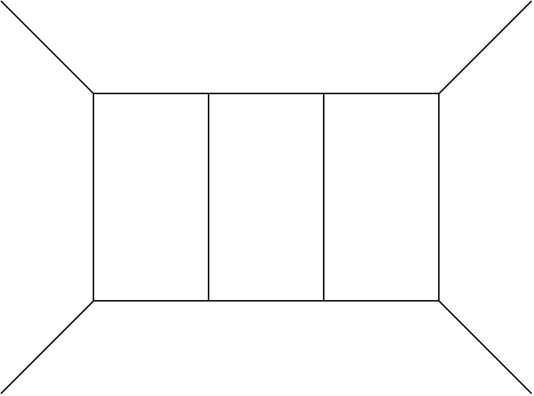
(PL)

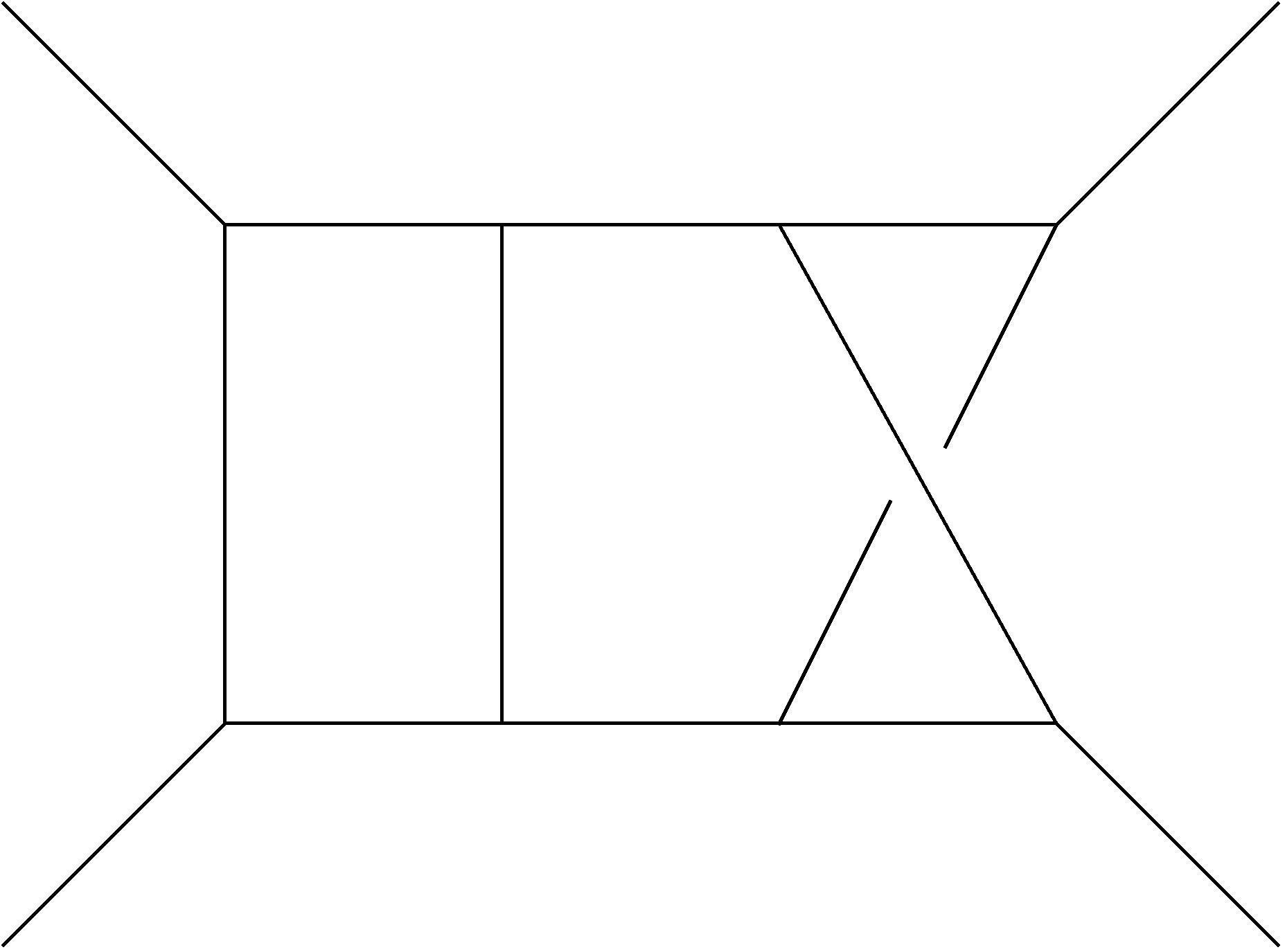
(NPL1)

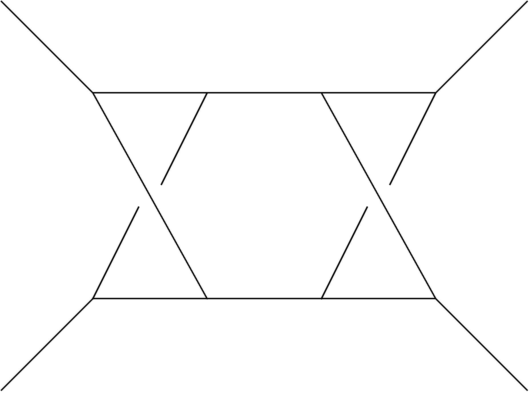
(NPL2)

Figure 1: Representative top level topologies for the planar (PL), single nonplanar (NPL1), and double nonplanar (NPL2) integral families.

We find it important to stress that by expressing the result for each $\overline{\mathcal{F}}_{1,...,8}$ in terms of a minimal set of integrals under crossings and shift symmetries, prior to performing the actual IBP reduction, we saw a significant decrease in complexity. This is expected, as many equivalent integrals are combined together and redundant structures are removed. After this simplification, we used the $\overline{\mathcal{F}}_{i}$ to construct the spinor-free helicity amplitudes, and collected the contributions to different colour structures. This way, we arrived at a minimal set of gauge-independent building blocks. We found it useful to partial fraction the rational functions with respect to $x$ in order to reduce their complexity.

The next step is the actual IBP integral reduction. We did this using an in-house implementation of the Laporta algorithm Laporta:2000dsw , Finred vonManteuffel:2016xki , which exploits syzygy-based techniques Gluza:2010ws ; Ita:2015tya ; Larsen:2015ped ; Bohm:2017qme ; Schabinger:2011dz ; Agarwal:2020dye and finite-field arithmetics vonManteuffel:2014ixa ; Peraro:2016wsq ; Peraro:2019svx ; vonManteuffel:2016xki . We found in this way that the three loop helicity amplitudes can be expressed in terms of the 221 MIs computed in ref. Henn:2020lye and crossed versions of them, for a total of $486$ MIs. We stress that these MIs are pure functions, i.e. they do not have any non-trivial rational functions of $x$ or $d$ as prefactors. Before inserting the IBP relations into the amplitude, we partial fractioned them with respect to both $d$ and $x$. We found that this step is crucial to keep the complexity under control. Finally, we performed one last partial fraction decomposition of the full amplitude after we wrote it in terms of MIs.

As a last step, we expand in $\epsilon$ and substitute the analytic results for the MIs. All of the integrals required for our calculation were computed in ref. Henn:2020lye . Their $\epsilon$ expansion can be written in terms of Harmonic Polylogarithms (HPL), that we define iteratively as

$$G(\underbrace{0,\dots,0}_{n~{}\text{times}};x)\equiv\frac{\ln^{n}x}{n!},~{}~{}~{}~{}~{}~{}~{}G(a_{n},...,a_{1};x)=\int_{0}^{x}\frac{dz}{z-a_{n}}G(a_{n-1},...,a_{1};z),$$ (32)

with $G(x)=1$ and $a_{i}\in\{0,1\}$. For our case, we need to consider polylogarithms up to weight 6, i.e. $n=6$ in eq. (32). We used the Mathematica package PolyLogTools Duhr:2019tlz to manipulate HPLs up to weight 5, augmented by a straightforward generalisation of its routines up to the required weight 6, as well as an independent package for multiple polylogarithms written by one of us. As expected from the fact that there are fewer weight $\leq 6$ HPLs than MIs, we observed a noticeable decrease in complexity for the amplitude after we expressed it in term of HPLs. We summarise the degree of complexity of the various steps discussed above in Tab. 1.

	1L	2L	3L
Number of diagrams	6	138	3299
Number of inequivalent integral families	1	2	3
Number of integrals before IBPs and symmetries	209	20935	4370070
Number of master integrals	6	39	486
Size of the Qgraf result [kB]	4	90	2820
Size of the Form result before IBPs and symmetries [kB]	276	54364	19734644
Size of helicity amplitudes written in terms of MIs [kB]	12	562	304409
Size of helicity amplitudes written in terms of HPLs [kB]	136	380	1195

Table 1: Complexity of the various stages of the calculation at different loop orders.

Before presenting our results, we note that although the MIs have been computed in ref. Henn:2020lye , for this calculation we have decided to recompute them as an independent check. We used the same definitions for the MIs as ref. Henn:2020lye , and followed the same strategy outlined in that reference for obtaining their analytic. First, since the basis Henn:2020lye is pure and of uniform weight Henn:2013pwa the MIs obey very simple differential equations

$$\mathrm{d}\vec{M}(\epsilon;s,t,u)=\epsilon\left[A_{s}\,\mathrm{d}\log(s)+A_{t}\,\mathrm{d}\log(t)+A_{u}\,\mathrm{d}\log(u)\right]\vec{M}(\epsilon;s,t,u),$$ (33)

where $\vec{M}$ is a vector whose components are the MIs and $A_{i}$ are constant matrices. Using the basis of ref. Henn:2020lye we have rederived the differential equation from scratch and found agreement. Given the simple form of eq. (33), it is straightforward to iteratively solve it order by order in $\epsilon$, modulo boundary conditions. The only non-trivial issue is how to fix the latter. Very interestingly, the authors of ref. Henn:2020lye noted that at three loops it is enough to impose regularity conditions to fix all boundary conditions, apart from one simple overall normalisation. The main idea is to look at the differential equation near singular points $s\to 0$, $t\to 0$, $u\to 0$. Let us consider $s\to 0$ as an example. In this limit the general solution of eq. (33) behaves like

$$\vec{M}\sim s^{A_{s}\epsilon}\vec{M}_{0,s},$$ (34)

where $\vec{M}_{0,s}$ is a constant vector. It was argued in ref. Henn:2020lye that the MIs considered here can only develop branch cuts of the form $s^{-\alpha\epsilon}$ with $\alpha>0$. This implies that the coefficient of $s^{\alpha\epsilon}$ in $s^{A_{s}\epsilon}\vec{M}_{0,s}$ must vanish for $\alpha>0$. As a consequence, there must exist non-trivial relations between different MIs in the $s\to 0$ limit. When combined with analogous relations derived from the limits $t,u\to 0$, the authors of ref. Henn:2020lye found that for the case under study one can completely constrain all the boundary conditions up to an overall normalisation factor. We have independently verified that this is the case, which allowed us to rederive an analytic expression for all the master integrals. We have then verified that our results to weight 6 are identical to the ones of ref. Henn:2020lye , provided that the latter are analytically continued to the physical Riemann sheet. Since in ref. Henn:2020lye final results are only presented for one single crossing, for convenience we decided to provide analytic results for all the three-loop master integrals and all their crossings in the ancillary files accompanying this publication. We also provide weight 6 results for a uniform-weight basis of the two-loop integrals.

5 UV renormalisation and IR regularisation

Following the steps outlined above, we obtained analytical expressions for the bare helicity amplitudes $f_{\vec{\lambda}}^{(L,b)}$ defined in eq. (27) for $L=1,2,3$. The $f_{\vec{\lambda}}^{(L,b)}$ are affected by both ultraviolet (UV) and infrared (IR) divergences, which manifest themselves as poles in the dimensional regularisation parameter $\epsilon=(4-d)/2$. While the former are removed by UV renormalisation, the latter can be regularised using universal IR operators acting on lower-loop amplitudes. We now discuss in detail how this can be done.

We first consider UV divergences. We define $\alpha_{s}(\mu)$ to be the renormalised strong coupling constant in the $\overline{\rm MS}$ scheme at the scale $\mu$

$$S_{\epsilon}\mu_{0}^{2\epsilon}\alpha_{s,b}=\mu^{2\epsilon}\alpha_{s}(\mu)Z[{\alpha_{s}(\mu)}],$$ (35)

with $S_{\epsilon}=(4\pi)^{\epsilon}e^{-\gamma_{E}\epsilon}$ and

$$Z[\alpha]=1-\frac{\beta_{0}}{\epsilon}\left(\frac{\alpha_{s}}{2\pi}\right)+\left(\frac{\beta_{0}^{2}}{\epsilon^{2}}-\frac{\beta_{1}}{2\epsilon}\right)\left(\frac{\alpha_{s}}{2\pi}\right)^{2}+\mathcal{O}(\alpha_{s}^{3}).$$ (36)

The first two coefficients of the QCD beta function read

$$\beta_{0}=\frac{11}{6}C_{A}-\frac{2}{3}T_{F}n_{f}\,,\qquad\beta_{1}=\frac{17}{6}C_{A}^{2}-T_{F}n_{f}\left(\frac{5}{3}C_{A}+C_{F}\right).$$ (37)

We then expand the spinor-free helicity amplitudes $f_{\vec{\lambda}}$ in terms of the renormalised strong coupling $\alpha_{s}(\mu)$ as

$$f_{\vec{\lambda}}=\sum_{L=1}^{3}\left(\frac{\alpha_{s}(\mu)}{2\pi}\right)^{L}f_{\vec{\lambda}}^{(L)}.$$ (38)

The expression for the renormalized amplitudes $f_{\vec{\lambda}}^{(L)}$ can be obtained by substituting eq. (35) in eq. (27) and expanding in the renormalised coupling. For convenience, we will set $\mu^{2}=s$ in the following. The result for arbitrary scale can be easily obtained using renormalisation group methods.

We now consider IR divergences. The IR structure of the amplitude is governed by the soft and collinear behaviour of virtual quarks and gluons and it is universal, i.e. it only depends on the colour and nature of the external legs. This allows one to write the renormalised amplitude as

$$f_{\vec{\lambda}}^{(1)} =f_{\vec{\lambda}}^{(1,{\rm fin})},$$

$$f_{\vec{\lambda}}^{(2)} =\mathcal{I}_{1}\,f_{\vec{\lambda}}^{(1)}+f_{\vec{\lambda}}^{(2,{\rm fin})},$$

$$f_{\vec{\lambda}}^{(3)} =\mathcal{I}_{2}\,f_{\vec{\lambda}}^{(1)}+\mathcal{I}_{1}\,f_{\vec{\lambda}}^{(2)}+f_{\vec{\lambda}}^{(3,{\rm fin})},$$ (39)

where $f_{\vec{\lambda}}^{(i,\rm fin)}$ are finite in four dimensions. The IR structure is encoded in the operators $\mathcal{I}_{i}$, that for our case (with $\mu^{2}=s$) read Catani:1998bh

$$\mathcal{I}_{1}(\epsilon) =-\frac{e^{i\pi\epsilon}e^{\gamma_{E}\epsilon}}{\Gamma(1-\epsilon)}\left(\frac{C_{A}}{\epsilon^{2}}+\frac{\beta_{0}}{\epsilon}\right),$$

$$\mathcal{I}_{2}(\epsilon) =-\frac{1}{2}\mathcal{I}_{1}(\epsilon)\left(\mathcal{I}_{1}(\epsilon)+\frac{2\beta_{0}}{\epsilon}\right)+\frac{e^{-\gamma_{E}\epsilon}\Gamma(1-2\epsilon)}{\Gamma(1-\epsilon)}\left(\frac{\beta_{0}}{\epsilon}+K\right)\mathcal{I}_{1}(2\epsilon)+2\frac{e^{\epsilon\gamma_{E}}}{\Gamma(1-\epsilon)}H_{g}\,,$$ (40)

where $K$ is the next-to-leading-order coefficient of the cusp anomalous dimension

$$K=\left(\frac{67}{18}-\frac{\pi^{2}}{6}\right)C_{A}-\frac{10}{9}n_{f}T_{F},$$ (41)

and Harlander:2000mg

$$H_{g}=\frac{1}{2\epsilon}\left[\left(\frac{\zeta(3)}{4}+\frac{5}{24}+\frac{11\pi^{2}}{288}\right)C_{A}^{2}+T_{F}n_{f}\left(\frac{C_{F}}{2}-\left(\frac{29}{27}+\frac{\pi^{2}}{72}\right)C_{A}\right)+\frac{10}{27}T_{F}^{2}n_{f}^{2}\right]\,.$$ (42)

In eqs (39) we used the fact that diphoton production in gluon fusion starts at one loop. The finite remainders for the helicity amplitudes $f_{\vec{\lambda}}^{(L,fin)}$ up to three loops are the main result of this paper, and we provide analytic results for them in the ancillary files.

6 Checks and structure of the result

We have performed various checks on the correctness of our results. First, we have employed two derivations of the three-loop $\mathcal{F}_{i}$ form factors at the integrand level and verified that they agree. We have also compared the one- and two-loop helicity amplitudes against the results of ref. Bern:2001df and found agreement. To validate our numerical evaluation procedure, we also checked the helicity-summed one-loop squared amplitude against OpenLoops Cascioli:2011va ; Buccioni:2019sur , and one helicity configuration at two loops against MCFM Campbell:2011bn ; Boughezal:2016wmq . Finally, we have verified that the UV and IR poles up to three loops follow the structure described in the previous section. This provides a strong check of the correctness of the three-loop amplitudes.

We now discuss the general structure of our result. The amplitude can be expressed in terms of the two quadratic Casimirs $C_{A}$ and $C_{F}$ and the flavour structures $n_{f}$, $n_{f}^{V}$ and $n_{f}^{V_{2}}$ defined in eq. (8). At $L$ loops the amplitude is a homogeneous degree-$L$ polynomial in these 5 variables. At one-loop, the amplitude is only proportional to $n_{f}^{V_{2}}$, since the two photons must both couple to the same fermion line. At two loops, the structures $n_{f}^{V_{2}}\times\{C_{F},C_{A}\}$ appear in the bare amplitude. The finite remainder contains in addition a term proportional to $n_{f}^{V_{2}}n_{f}$ stemming from $\beta_{0}$ in the UV/IR regularisation. We note that there is no $(n_{f}^{V})^{2}$ contribution. It is easy to understand why this is the case. The $(n_{f}^{V})^{2}$ colour factor only appears if the two photons are attached to two different (closed) fermion lines. Such diagrams do appear at two loops, but they are of the form of two $\gamma gg^{*}$ one-loop triangles connected through a gluon propagator. Due to an argument analogous to Furry’s theorem, these diagrams give no net contribution to the amplitude. A similar argument allows one to conclude that there is no net contribution from Feynman diagrams with colour factors $n_{f}(n_{f}^{V})^{2}$ at three loops. Furthermore, it is easy to see that the structure $n_{f}^{2}n_{f}^{V_{2}}$ is absent in the three-loop bare amplitude. Since there is no $(n_{f}^{V})^{2}$ contribution at lower loops, the $(n_{f}^{V})^{2}$ term in the bare three loop amplitude must be finite. We observe, however, that it is non-zero. Indeed, at three loops this colour factor appears in triple-box diagrams for which the Furry argument outlined above is no longer applicable.

We now move to the discussion of the kinematic features of the three-loop amplitude, i.e. its $x$ dependence. The amplitude contains terms of the form $G(a_{1},...,a_{n};x)/x^{k}$ ($-2\leq k\leq 2$) and $G(a_{1},...,a_{n};x)/(1-x)^{k}$ ($1\leq k\leq 2$) , where $a_{i}\in\{0,1\}$, $0\leq n\leq 6$, and $G$ are the Harmonic Polylogarithms defined in eq. (32). Instead of the HPLs, we found it useful to also consider the alternative functional basis described in ref. Caola:2020dfu to speed up the numerical evaluation of the final result. Using the algorithm of Duhr:2011zq , we have constructed a basis of logarithms, classical polylogarithms and multiple polylogarithms to rewrite the HPLs without introducing any new spurious singularities. We used products of lower weight functions whenever possible and preferred functions whose series representation requires a small number of nested sums. In this way, we found that 23 independent transcendental functions and products thereof suffice to represent our HPLs up to weight 6. The new basis consists of 2 logarithms, $\ln(x)$ $\ln(1-x)$, 12 classical polylogarithms, $\operatorname{Li}_{2}$ of $x$, $\operatorname{Li}_{3}$ of $x$ and $1-x$ and $\operatorname{Li}_{4}$, $\operatorname{Li}_{5}$, $\operatorname{Li}_{6}$ of $x,1-x$ and $-x/(1-x)$, as well as 9 multiple polylogarithms $\operatorname{Li}_{3,2}(1,x),\operatorname{Li}_{3,2}(1-x,1),\operatorname{Li}_{3,2}(x,1),\operatorname{Li}_{3,3}(1-x,1),\operatorname{Li}_{3,3}(x,1),\operatorname{Li}_{3,3}\left(\frac{-x}{1-x},1\right),\operatorname{Li}_{4,2}(1-x,1),\operatorname{Li}_{4,2}(x,1),\operatorname{Li}_{2,2,2}(x,1,1)$. Here, we follow the conventions of ref. Vollinga:2004sn and define

$$\operatorname{Li}_{m_{1},...,m_{k}}(x_{1},...,x_{k})=\sum_{i_{1}>...>i_{k}>0}\frac{x_{1}^{i_{1}}}{i_{1}^{m_{1}}}\,...\,\frac{x_{k}^{i_{k}}}{i_{k}^{m_{k}}}\,.$$ (43)

In the ancillary files, we provide our analytic results written both in terms of HPLs and in terms of this minimal set of functions. For convenience, we also provide results for the finite remainders of the one- and two-loop helicity amplitudes up to weight 6.

Finally, we present our results. Although intermediate expressions are rather complicated, see Table 1, we find that the final results are remarkably compact. The ${\vec{\lambda}}=(++++)$ helicity configuration is particularly simple. This is of course expected, since the one-loop amplitude does not have support on any cut, hence it is purely rational rather than a weight-2 function. This simplicity persists at higher loops. For illustration, we now report here the result for the finite reminders defined in eq. (39) up to three loops for this helicity configuration. At one and two loops one has

$$f^{(1,{\rm fin})}_{++++} =2n_{f}^{V_{2}},$$ (44)

$$f^{(2,{\rm fin})}_{++++} =2n_{f}^{V_{2}}\left(2C_{A}-3C_{F}+i\pi\beta_{0}\right).$$ (45)

At three loops, we write the finite remainder as

$$f^{(3,{\rm fin})}_{++++} =\Delta_{1}(x)\,n_{f}^{V_{2}}C_{A}^{2}+\Delta_{2}(x)\,n_{f}^{V_{2}}C_{A}C_{F}+\Delta_{3}(x)\,n_{f}n_{f}^{V_{2}}C_{A}+\Delta_{4}(x)\,(n_{f}^{V})^{2}C_{A}$$

$$\quad+\Delta_{5}(x)\,n_{f}^{V_{2}}C_{F}^{2}+\Delta_{6}(x)\,(n_{f}^{V})^{2}C_{F}+\Delta_{7}(x)\,n_{f}n_{f}^{V_{2}}C_{F}+\Delta_{8}(x)\,n_{f}^{2}n_{f}^{V_{2}}$$

$$\quad+\{(x)\leftrightarrow(1-x)\}$$ (46)

with

$$\Delta_{1}(x) =-\mfrac{23L_{1}(L_{1}+2i\pi)}{9x^{2}}+\mfrac{32L_{1}(L_{1}+2i\pi)-46(L_{1}+i\pi)}{9x}-\mfrac{17}{36}L_{0}^{2}-\mfrac{19}{36}L_{0}L_{1}+\mfrac{1}{9}L_{0}-2i\pi L$$

$$\quad+\mfrac{1}{288}\pi^{4}-\mfrac{373}{72}\zeta_{3}-\mfrac{185}{72}\pi^{2}+\mfrac{4519}{324}+\mfrac{1}{2}i\pi\zeta_{3}+\mfrac{11}{144}i\pi^{3}+\mfrac{157}{12}i\pi+\mfrac{43}{9}L_{0}x$$

$$\quad-\mfrac{7}{9}x^{2}\left((L_{0}-L_{1})^{2}+\pi^{2}\right)\,,$$

$$\Delta_{2}(x) =\mfrac{8L_{1}(L_{1}+2i\pi)}{3x^{2}}+\mfrac{16(L_{1}+i\pi)-{8}L_{1}(L_{1}+2i\pi)}{3x}-\mfrac{1}{3}L_{0}^{2}+\mfrac{5}{6}L_{0}L_{1}+\mfrac{17}{3}L_{0}+i\pi L_{0}-\mfrac{5}{12}\pi^{2}$$

$$\quad-\mfrac{199}{6}-{8}i\pi-\mfrac{16}{3}L_{0}x+\mfrac{4}{3}x^{2}\left((L_{0}-L_{1})^{2}+\pi^{2}\right)\,,$$

$$\Delta_{3}(x) =\mfrac{L_{1}(L_{1}+2i\pi)}{18x^{2}}+\mfrac{2(L_{1}+i\pi)-L_{1}(L_{1}+2i\pi)}{18x}-\mfrac{1}{36}L_{0}^{2}+\mfrac{1}{36}L_{0}L_{1}-\mfrac{1}{9}L_{0}-\mfrac{61}{36}\zeta_{3}+\mfrac{475}{432}\pi^{2}$$

$$\quad-\mfrac{925}{324}-\mfrac{1}{72}i\pi^{3}-\mfrac{175}{54}i\pi+\mfrac{2}{9}L_{0}x+\mfrac{1}{36}x^{2}\left((L_{0}-L_{1})^{2}+\pi^{2}\right)\,,$$

$$\Delta_{4}(x) =-\mfrac{5L_{1}(L_{1}+2i\pi)}{4x^{2}}+\mfrac{L_{1}(L_{1}+2i\pi)-8(L_{1}+i\pi)}{2x}+\mfrac{1}{4}L_{0}^{2}-\mfrac{1}{4}L_{0}L_{1}-{2}L_{0}-{6}\zeta_{3}+\mfrac{1}{8}\pi^{2}-\mfrac{1}{2}$$

$$\quad+{4}L_{0}x-x^{2}\left((L_{0}-L_{1})^{2}+\pi^{2}\right)\,,$$

$$\Delta_{5}(x) =-\mfrac{L_{1}(L_{1}+2i\pi)}{x^{2}}+\mfrac{L_{1}(L_{1}+2i\pi)-2(L_{1}+i\pi)}{x}-\mfrac{1}{2}L_{0}^{2}-i\pi L_{0}+\mfrac{39}{4}+i\pi+{2}L_{0}x$$

$$\quad-\mfrac{1}{2}x^{2}\left((L_{0}-L_{1})^{2}+\pi^{2}\right)\,,$$

$$\Delta_{6}(x) =\mfrac{10L_{1}(L_{1}+2i\pi)}{3x^{2}}+\mfrac{32(L_{1}+i\pi)-{4}L_{1}(L_{1}+2i\pi)}{3x}-\mfrac{2}{3}L_{0}^{2}+\mfrac{2}{3}L_{0}L_{1}+\mfrac{16}{3}L_{0}+{16}\zeta_{3}-\mfrac{1}{3}\pi^{2}$$

$$\quad+\mfrac{4}{3}-\mfrac{32}{3}L_{0}x+\mfrac{8}{3}x^{2}\left((L_{0}-L_{1})^{2}+\pi^{2}\right)\,,$$

$$\Delta_{7}(x) =\mfrac{5L_{1}(L_{1}+2i\pi)}{3x^{2}}+\mfrac{10(L_{1}+i\pi)-8L_{1}(L_{1}+2i\pi)}{3x}+\mfrac{2}{3}L_{0}^{2}+\mfrac{1}{3}L_{0}L_{1}-\mfrac{10}{3}L_{0}+2i\pi L_{0}+{4}\zeta_{3}$$

$$\quad-\mfrac{\pi^{2}}{6}+{5}-{3}i\pi-\mfrac{10}{3}L_{0}x+\mfrac{1}{3}x^{2}\left((L_{0}-L_{1})^{2}+\pi^{2}\right)\,,$$

$$\Delta_{8}(x) =-\mfrac{23}{216}\pi^{2}+\mfrac{5}{27}i\pi\,.$$ (47)

In eq. (47), we have defined $L_{0}=\ln(x)$ and $L_{1}=\ln(1-x)$. We note that these are the only transcendental functions that are needed to describe our result.

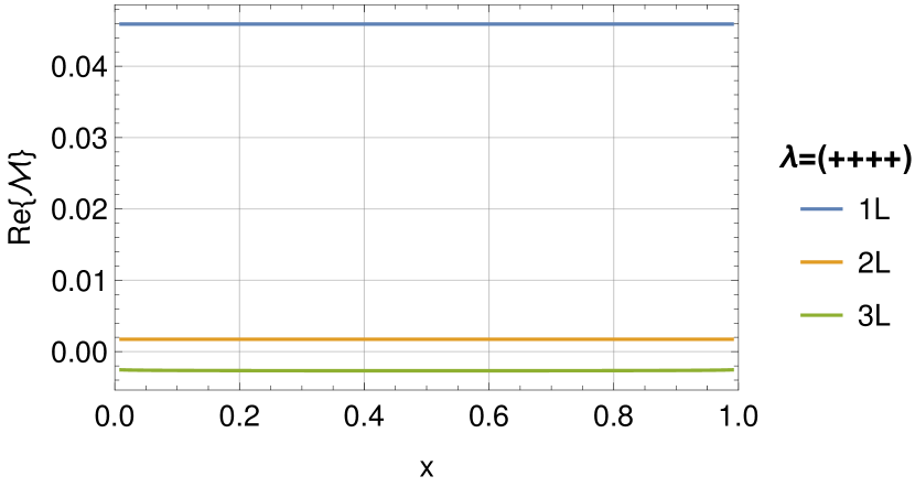
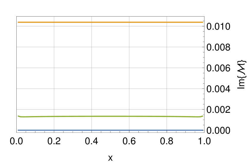
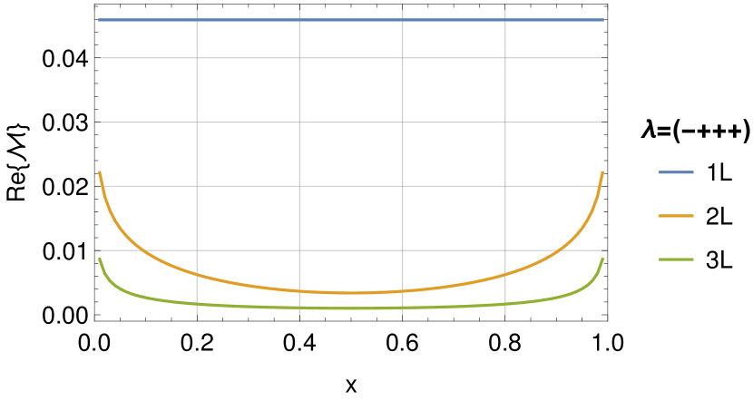
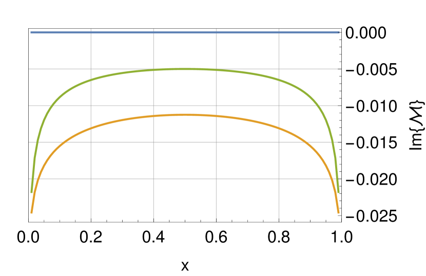
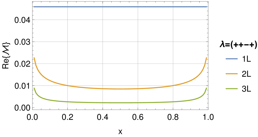
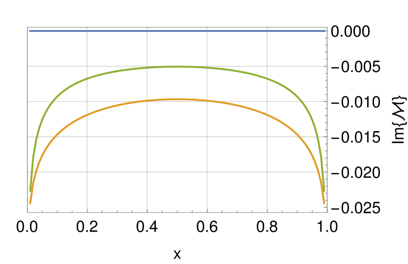
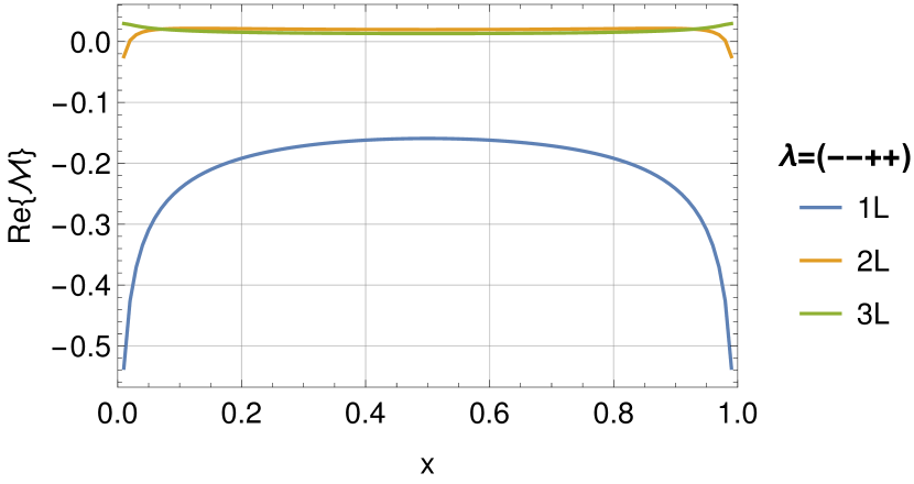
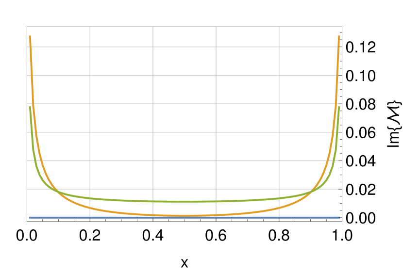
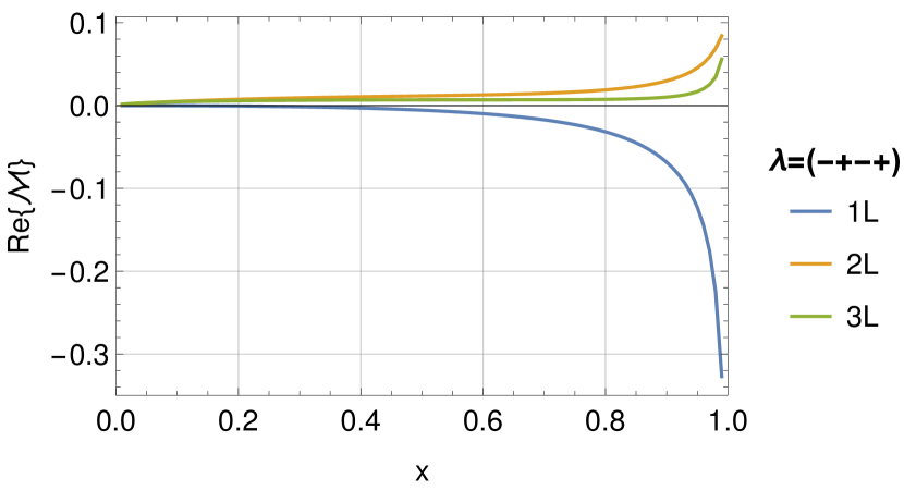
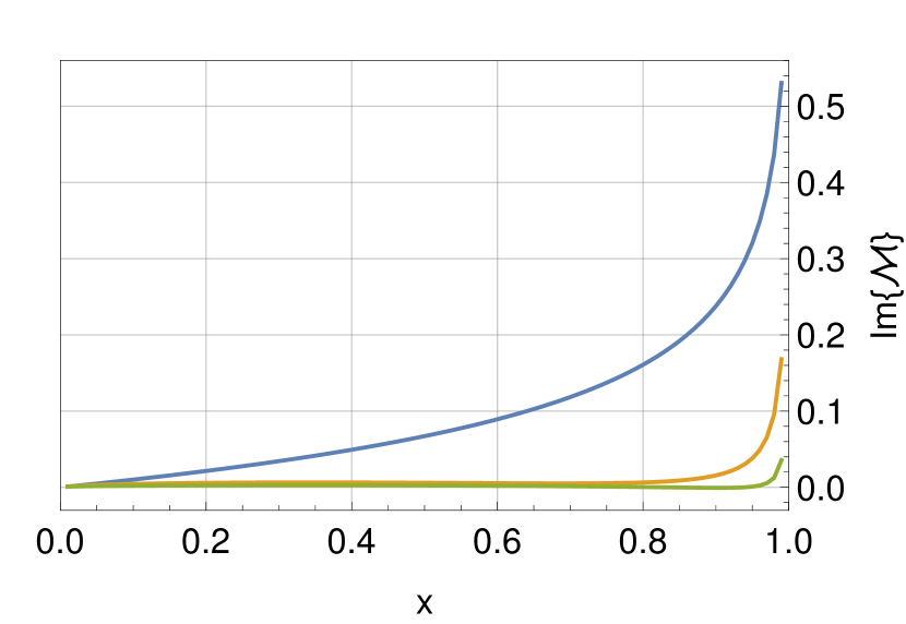
Figure 2: Finite remainders $\mathcal{M}^{(L)}_{\vec{\lambda}}\equiv\left(\frac{\alpha_{s}}{2\pi}\right)^{L}\,f^{(L,{\rm fin})}_{\vec{\lambda}}$ as functions of $x=-t/s$.

Although the results for the remaining helicity configurations are still rather compact, they are much larger than for the ${\vec{\lambda}}=(++++)$ case. We provide them in electronically-readable format, attached the arXiv submission of this paper. In Figure 2 we plot our result for the one-, two- and three-loop finite remainders $\mathcal{M}^{(L)}_{\vec{\lambda}}\equiv\left(\frac{\alpha_{s}}{2\pi}\right)^{L}f_{\vec{\lambda}}^{(L,\rm fin)}$ as functions of $x$. We fix $\alpha_{s}=0.118$ and show graphs for the helicity configurations ${\vec{\lambda}}=(++++)$, $(-+++)$, $(++-+)$, $(--++)$ and $(-+-+)$. All the other helicity amplitudes can be obtained from these through Bose symmetry ($x\leftrightarrow 1-x$) and parity.

7 Conclusions

In this paper, we have computed the helicity amplitudes for the process $gg\to\gamma\gamma$ in three-loop massless QCD. This is the last missing ingredient required for the calculation of the NNLO QCD corrections to diphoton production in the $gg$ channel. For our analytical three-loop calculation, we have adopted a new projector-based prescription to compute helicity amplitudes in the ’t Hooft-Veltman scheme. The expressions at the intermediate stages of our calculation were quite sizable, and we employed recent ideas for the demanding integration-by-parts reductions. Our final results though are remarkably compact. They can be expressed either in terms of standard Harmonic Polylogarithms of weight up to six, or in terms of only 23 transcendental functions defined by up to three-fold sums. This makes the numerical evaluation of our result both fast and numerically stable. Analytical results for both choices of the transcendental functions are provided in the ancillary files that accompany this publication.

We envision several possible future directions of investigations. On a more phenomenological side, it would be interesting to combine our results with those of refs Badger:2021imn ; Badger:2021ohm to obtain NNLO predictions for the $gg\to\gamma\gamma$ process. On a more theoretical side, the simplicity of our final results begs for an exploration of new ways to perform multiloop calculations. Finally, it would be very interesting to promote our calculation to the fully non-abelian case and consider three-loop scattering amplitudes for the $gg\to gg$ process. We look forward to pursuing these lines of investigation in the future.

References

- (1) S. Frixione, Isolated photons in perturbative QCD, Phys. Lett. B 429 (1998) 369–374, [hep-ph/9801442].
- (2) S. Catani, L. Cieri, D. de Florian, G. Ferrera and M. Grazzini, Diphoton production at hadron colliders: a fully-differential QCD calculation at NNLO, Phys. Rev. Lett. 108 (2012) 072001, [1110.2375].
- (3) F. Caola, A. Chakraborty, G. Gambuti, A. von Manteuffel and L. Tancredi, Three-loop helicity amplitudes for four-quark scattering in massless QCD, JHEP 10 (2021) 206, [2108.00055].
- (4) H. A. Chawdhry, M. L. Czakon, A. Mitov and R. Poncelet, NNLO QCD corrections to three-photon production at the LHC, JHEP 02 (2020) 057, [1911.00479].
- (5) H. A. Chawdhry, M. Czakon, A. Mitov and R. Poncelet, Two-loop leading-color helicity amplitudes for three-photon production at the LHC, JHEP 06 (2021) 150, [2012.13553].
- (6) H. A. Chawdhry, M. Czakon, A. Mitov and R. Poncelet, Two-loop leading-colour QCD helicity amplitudes for two-photon plus jet production at the LHC, JHEP 07 (2021) 164, [2103.04319].
- (7) H. A. Chawdhry, M. Czakon, A. Mitov and R. Poncelet, NNLO QCD corrections to diphoton production with an additional jet at the LHC, 2105.06940.
- (8) B. Agarwal, F. Buccioni, A. von Manteuffel and L. Tancredi, Two-loop leading colour QCD corrections to and , JHEP 04 (2021) 201, [2102.01820].
- (9) B. Agarwal, F. Buccioni, A. von Manteuffel and L. Tancredi, Two-loop helicity amplitudes for diphoton plus jet production in full color, 2105.04585.
- (10) S. Badger, C. Brønnum-Hansen, D. Chicherin, T. Gehrmann, H. B. Hartanto, J. Henn et al., Virtual QCD corrections to gluon-initiated diphoton plus jet production at hadron colliders, 2106.08664.
- (11) S. Badger, T. Gehrmann, M. Marcoli and R. Moodie, Next-to-leading order QCD corrections to diphoton-plus-jet production through gluon fusion at the LHC, 2109.12003.
- (12) C. Anastasiou, E. W. N. Glover and M. E. Tejeda-Yeomans, Two loop QED and QCD corrections to massless fermion boson scattering, Nucl. Phys. B 629 (2002) 255–289, [hep-ph/0201274].
- (13) J. M. Campbell, R. K. Ellis, Y. Li and C. Williams, Predictions for diphoton production at the LHC through NNLO in QCD, JHEP 07 (2016) 148, [1603.02663].
- (14) T. Gehrmann, N. Glover, A. Huss and J. Whitehead, Scale and isolation sensitivity of diphoton distributions at the LHC, JHEP 01 (2021) 108, [2009.11310].
- (15) M. Grazzini, S. Kallweit and M. Wiesemann, Fully differential NNLO computations with MATRIX, Eur. Phys. J. C 78 (2018) 537, [1711.06631].
- (16) S. Alioli, A. Broggio, A. Gavardi, S. Kallweit, M. A. Lim, R. Nagar et al., Precise predictions for photon pair production matched to parton showers in GENEVA, JHEP 04 (2021) 041, [2010.10498].
- (17) T. Neumann, The diphoton spectrum at N3LL′ + NNLO, Eur. Phys. J. C 81 (2021) 905, [2107.12478].
- (18) Z. Bern, A. De Freitas and L. J. Dixon, Two loop amplitudes for gluon fusion into two photons, JHEP 09 (2001) 037, [hep-ph/0109078].
- (19) Z. Bern, L. J. Dixon and C. Schmidt, Isolating a light Higgs boson from the diphoton background at the CERN LHC, Phys. Rev. D 66 (2002) 074018, [hep-ph/0206194].
- (20) CMS collaboration, S. Chatrchyan et al., Measurement of differential cross sections for the production of a pair of isolated photons in pp collisions at , Eur. Phys. J. C 74 (2014) 3129, [1405.7225].
- (21) ATLAS collaboration, G. Aad et al., Measurement of the production cross section of pairs of isolated photons in collisions at 13 TeV with the ATLAS detector, 2107.09330.
- (22) S. P. Martin, Shift in the LHC Higgs Diphoton Mass Peak from Interference with Background, Phys. Rev. D 86 (2012) 073016, [1208.1533].
- (23) L. J. Dixon and Y. Li, Bounding the Higgs Boson Width Through Interferometry, Phys. Rev. Lett. 111 (2013) 111802, [1305.3854].
- (24) LHC Higgs Cross Section Working Group collaboration, D. de Florian et al., Handbook of LHC Higgs Cross Sections: 4. Deciphering the Nature of the Higgs Sector, 1610.07922.
- (25) S. P. Martin, Interference of Higgs Diphoton Signal and Background in Production with a Jet at the LHC, Phys. Rev. D 88 (2013) 013004, [1303.3342].
- (26) D. de Florian, N. Fidanza, R. J. Hernández-Pinto, J. Mazzitelli, Y. Rotstein Habarnau and G. F. R. Sborlini, A complete calculation of the signal-background interference for the Higgs diphoton decay channel, Eur. Phys. J. C 73 (2013) 2387, [1303.1397].
- (27) F. Coradeschi, D. de Florian, L. J. Dixon, N. Fidanza, S. Höche, H. Ita et al., Interference effects in the jets channel at the LHC, Phys. Rev. D 92 (2015) 013004, [1504.05215].
- (28) J. Campbell, M. Carena, R. Harnik and Z. Liu, Interference in the On-Shell Rate and the Higgs Boson Total Width, Phys. Rev. Lett. 119 (2017) 181801, [1704.08259].
- (29) T. Peraro and L. Tancredi, Physical projectors for multi-leg helicity amplitudes, JHEP 07 (2019) 114, [1906.03298].
- (30) T. Peraro and L. Tancredi, Tensor decomposition for bosonic and fermionic scattering amplitudes, Phys. Rev. D 103 (2021) 054042, [2012.00820].
- (31) G. ’t Hooft and M. Veltman, Regularization and renormalization of gauge fields, Nuclear Physics B 44 (1972) 189–213.
- (32) T. Binoth, E. W. N. Glover, P. Marquard and J. J. van der Bij, Two loop corrections to light by light scattering in supersymmetric QED, JHEP 05 (2002) 060, [hep-ph/0202266].
- (33) L. J. Dixon, Calculating scattering amplitudes efficiently, in Theoretical Advanced Study Institute in Elementary Particle Physics (TASI 95): QCD and Beyond, 1, 1996. hep-ph/9601359.
- (34) J. Henn, B. Mistlberger, V. A. Smirnov and P. Wasser, Constructing d-log integrands and computing master integrals for three-loop four-particle scattering, JHEP 04 (2020) 167, [2002.09492].
- (35) F. Caola, A. Von Manteuffel and L. Tancredi, Diphoton Amplitudes in Three-Loop Quantum Chromodynamics, Phys. Rev. Lett. 126 (2021) 112004, [2011.13946].
- (36) K. G. Chetyrkin and F. V. Tkachov, Integration by Parts: The Algorithm to Calculate beta Functions in 4 Loops, Nucl. Phys. B 192 (1981) 159–204.
- (37) S. Laporta, High precision calculation of multiloop Feynman integrals by difference equations, Int. J. Mod. Phys. A 15 (2000) 5087–5159, [hep-ph/0102033].
- (38) P. Nogueira, Automatic Feynman graph generation, J. Comput. Phys. 105 (1993) 279–289.
- (39) A. von Manteuffel and C. Studerus, Reduze 2 - Distributed Feynman Integral Reduction, 1201.4330.
- (40) C. Studerus, Reduze-Feynman Integral Reduction in C++, Comput. Phys. Commun. 181 (2010) 1293–1300, [0912.2546].
- (41) J. A. M. Vermaseren, New features of FORM, math-ph/0010025.
- (42) A. von Manteuffel and R. M. Schabinger, Quark and gluon form factors to four-loop order in QCD: the contributions, Phys. Rev. D 95 (2017) 034030, [1611.00795].
- (43) J. Gluza, K. Kajda and D. A. Kosower, Towards a Basis for Planar Two-Loop Integrals, Phys. Rev. D 83 (2011) 045012, [1009.0472].
- (44) H. Ita, Two-loop Integrand Decomposition into Master Integrals and Surface Terms, Phys. Rev. D 94 (2016) 116015, [1510.05626].
- (45) K. J. Larsen and Y. Zhang, Integration-by-parts reductions from unitarity cuts and algebraic geometry, Phys. Rev. D 93 (2016) 041701, [1511.01071].
- (46) J. Böhm, A. Georgoudis, K. J. Larsen, M. Schulze and Y. Zhang, Complete sets of logarithmic vector fields for integration-by-parts identities of Feynman integrals, Phys. Rev. D 98 (2018) 025023, [1712.09737].
- (47) R. M. Schabinger, A New Algorithm For The Generation Of Unitarity-Compatible Integration By Parts Relations, JHEP 01 (2012) 077, [1111.4220].
- (48) B. Agarwal, S. P. Jones and A. von Manteuffel, Two-loop helicity amplitudes for with full top-quark mass effects, JHEP 05 (2021) 256, [2011.15113].
- (49) A. von Manteuffel and R. M. Schabinger, A novel approach to integration by parts reduction, Phys. Lett. B 744 (2015) 101–104, [1406.4513].
- (50) T. Peraro, Scattering amplitudes over finite fields and multivariate functional reconstruction, JHEP 12 (2016) 030, [1608.01902].
- (51) T. Peraro, FiniteFlow: multivariate functional reconstruction using finite fields and dataflow graphs, JHEP 07 (2019) 031, [1905.08019].
- (52) J. Vollinga and S. Weinzierl, Numerical evaluation of multiple polylogarithms, Comput. Phys. Commun. 167 (2005) 177, [hep-ph/0410259].
- (53) T. Gehrmann and E. Remiddi, Numerical evaluation of harmonic polylogarithms, Comput. Phys. Commun. 141 (2001) 296–312, [hep-ph/0107173].
- (54) C. Duhr and F. Dulat, PolyLogTools — polylogs for the masses, JHEP 08 (2019) 135, [1904.07279].
- (55) J. M. Henn, Multiloop integrals in dimensional regularization made simple, Phys. Rev. Lett. 110 (2013) 251601, [1304.1806].
- (56) S. Catani, The Singular behavior of QCD amplitudes at two loop order, Phys. Lett. B 427 (1998) 161–171, [hep-ph/9802439].
- (57) R. V. Harlander, Virtual corrections to g g — H to two loops in the heavy top limit, Phys. Lett. B 492 (2000) 74–80, [hep-ph/0007289].
- (58) F. Cascioli, P. Maierhofer and S. Pozzorini, Scattering Amplitudes with Open Loops, Phys. Rev. Lett. 108 (2012) 111601, [1111.5206].
- (59) F. Buccioni, J.-N. Lang, J. M. Lindert, P. Maierhöfer, S. Pozzorini, H. Zhang et al., OpenLoops 2, Eur. Phys. J. C 79 (2019) 866, [1907.13071].
- (60) J. M. Campbell, R. K. Ellis and C. Williams, Vector boson pair production at the LHC, JHEP 07 (2011) 018, [1105.0020].
- (61) R. Boughezal, J. M. Campbell, R. K. Ellis, C. Focke, W. Giele, X. Liu et al., Color singlet production at NNLO in MCFM, Eur. Phys. J. C 77 (2017) 7, [1605.08011].
- (62) C. Duhr, H. Gangl and J. R. Rhodes, From polygons and symbols to polylogarithmic functions, JHEP 1210 (2012) 075, [1110.0458].
- (63) D. Binosi and L. Theussl, JaxoDraw: A Graphical user interface for drawing Feynman diagrams, Comput. Phys. Commun. 161 (2004) 76–86, [hep-ph/0309015].
- (64) J. A. M. Vermaseren, Axodraw, Comput. Phys. Commun. 83 (1994) 45–58.