Fusion of Sensor Measurements and
Target-Provided Information in Multitarget Tracking

Abstract

Tracking multiple time-varying states based on heterogeneous observations is a key problem in many applications. Here, we develop a statistical model and algorithm for tracking an unknown number of targets based on the probabilistic fusion of observations from two classes of data sources. The first class, referred to as target-independent perception systems (TIPSs), consists of sensors that periodically produce noisy measurements of targets without requiring target cooperation. The second class, referred to as target-dependent reporting systems (TDRSs), relies on cooperative targets that report noisy measurements of their state and their identity. We present a joint TIPS–TDRS observation model that accounts for observation-origin uncertainty, missed detections, false alarms, and asynchronicity. We then establish a factor graph that represents this observation model along with a state evolution model including target identities. Finally, by executing the sum-product algorithm on that factor graph, we obtain a scalable multitarget tracking algorithm with inherent TIPS–TDRS fusion. The performance of the proposed algorithm is evaluated using simulated data as well as real data from a maritime surveillance experiment.

I Introduction

Multitarget tracking (MTT) consists in estimating the number and the time-varying states of multiple moving objects (targets) [1, 2, 3, 4, 5, 6]. To obtain satisfactory performance, it is often necessary to fuse information from multiple heterogeneous data sources. Indeed, heterogeneous data fusion for MTT is a key task for many applications including surveillance, robotics, and remote sensing [2, 3, 4].

I-A TIPS and TDRS

In this paper, we focus on the fusion of observations produced by two different classes of data sources, with the objective of improving the overall MTT capabilities. The first class will be referred to as target-independent perception systems (TIPSs). A TIPS consists of one or multiple sensors that rely on an active and periodic interrogation of the environment to acquire target-related measurements. Due to this active interrogation, a TIPS can also acquire measurements related to targets that do not cooperate in any form. Active interrogation is based on signals that are either transmitted by the TIPS itself or are signals of opportunity transmitted by other sources. The sensors constituting a TIPS may be heterogeneous and with different sensing modalities, e.g., radars, optical cameras, and sonars [7]. The TIPS measurements are extracted in a preprocessing step from a noisy received signal. As a consequence, they are themselves noisy. Furthermore, due to errors made in the preprocessing step, certain measurements may not originate from a target (false alarms) and certain targets may not generate measurements (missed detections) [5, 6]. Since the targets do not cooperate, there is a TIPS measurement-origin uncertainty, i.e., it is not clear if a given TIPS measurement was generated by a target, and by which target.

The second class of data sources will be referred to as target-dependent reporting systems (TDRSs). A TDRS relies on information autonomously transmitted by cooperative targets: each cooperative target is equipped with a transmitter, which is identified by a code or ID, and transmits messages to the TDRS—called reports—that include the ID and a noisy measurement of the target state. Reports are received asynchronously by the TDRS; moreover, due to imperfect communication channels between the cooperative targets and the TDRS, a report may be lost, i.e., not received at all, or it may be received but contain a corrupted ID and/or measurement. Because of such corrupted IDs, the association between cooperative targets and reports is uncertain; this is similar to the TIPS measurement-origin uncertainty. However, each report must originate from a cooperative target, i.e., it cannot be a false alarm.

TIPSs and TDRSs arise in many applications. For example, in the maritime domain, coastal/harbor radars are TIPS sensors and the automatic identification system (AIS) [8] is a TDRS, and in air traffic control, primary surveillance radars are TIPS sensors and the automatic dependent surveillance broadcast (ADS-B) system [9] is a TDRS. TIPSs and TDRSs are mostly used as stand-alone systems, and the information they provide is usually combined by fusing the respective estimates of the target tracks [10, 11, 12, 13, 14, 15]. In this paper, by contrast, we address the estimation of the target states directly from the heterogeneous TIPS-TDRS observations. This approach, which is known as observation-level fusion, can be expected to yield better performance [16]. An MTT algorithm fusing the observations from a single radar sensor and the AIS has been proposed in [17]. This algorithm uses a joint probabilistic data association technique to cope with the unknown associations between targets and radar measurements as well as between targets and IDs, along with a gating technique to reduce the number of admissible associations. However, the radar and AIS observations are assumed to be based on synchronous clocks, and the radar measurement rate is assumed to be a multiple of the AIS report rate. In practice, these assumptions are often not satisfied.

I-B Contributions and Paper Organization

In our previous work [18, 19, 20], we presented an MTT algorithm that fuses measurements from multiple TIPS sensors and is able to confirm the existence of an unknown and time-varying number of targets and track the target states in the presence of TIPS measurement-origin uncertainty, missed detections, and false alarms. This algorithm was derived by formulating the multisensor MTT problem in a Bayesian framework, representing the factorization of the joint posterior distribution by a factor graph, and efficiently marginalizing the joint posterior distribution via the sum-product algorithm (SPA) [21, 22]. The SPA exploits conditional statistical independences for a drastic reduction of complexity. This results in an excellent scalability of the MTT algorithm of [18, 19] with respect to the number of targets, the number of TIPS sensors, and the number of measurements per sensor. We note that an alternative framework for the development of MTT algorithms is constituted by random finite sets (RFSs) [23, 24, 25]. Similarities and differences of an SPA-based derivation of MTT methods relative to an RFS-based derivation are discussed in [19].

Here, we propose an SPA-based framework and algorithm for MTT with TIPS-TDRS fusion. More specifically, we extend the MTT framework and algorithm of [18] to incorporate reports provided by a TDRS. Our key contributions are as follows:

• We establish a statistical model of MTT based on measurements provided by multiple TIPS sensors and reports provided by a TDRS. The TDRS reports are asynchronous and include the IDs from cooperative targets.

• We represent this statistical model by a factor graph and use the SPA to develop a scalable message passing algorithm for MTT with TIPS-TDRS fusion.

• We demonstrate performance advantages of MTT with TIPS-TDRS fusion using simulated data, and validate the proposed algorithm on real data from a maritime surveillance experiment.

Parts of this work were presented in our conference publications [26] and [27]. This paper differs from those publications in that it extends the formulation beyond the maritime (i.e., AIS) domain; it introduces an improved modeling for the TDRS IDs; it presents detailed derivations of the joint posterior distribution; it presents the SPA messages in a more complete and detailed manner; and it validates the performance of the proposed MTT algorithm in an additional simulated scenario and in a real maritime scenario.

The remainder of the paper is organized as follows. The basic notation and nomenclature are described in the next subsection. Section II introduces the TIPS-TDRS fusion problem and outlines the proposed approach. The system model and its statistical formulation are described in Section III. In Section IV, we derive the joint posterior distribution and the corresponding factor graph. The proposed message passing algorithm is presented in Section V. Section VI provides an extensive evaluation of the proposed algorithm using simulated data. Section VII presents an application using real data from a maritime surveillance experiment.

I-C Notation and Nomenclature

Vectors are denoted by boldface lower-case letters (e.g., $\bm{a}$), matrices by boldface upper-case letters (e.g., $\bm{A}$), and sets by calligraphic letters (e.g., $\mathcal{A}$). The transpose is written as $(\cdot)^{\raisebox{0.0pt}[0.0pt][0.0pt]{\scriptsize{{t}}}}\!$. The Euclidean norm of vector $\bm{a}$ is denoted by $\left\|\bm{a}\right\|$. For a two-dimensional (2D) vector $\bm{a}$, $\angle\bm{a}$ is the angle defined clockwise and such that $\angle\bm{a}\!=\!0$ for $\bm{a}=[0\,\,1]^{\raisebox{0.0pt}[0.0pt][0.0pt]{\scriptsize{{t}}}}$. We write $\mathrm{diag}(a_{1},\ldots,$$a_{N})$ for an $N\!\times N$ diagonal matrix with diagonal entries $a_{1},\ldots,$$a_{N}$, ${\bf I}_{N}$ for the $N\!\times\!N$ identity matrix, and $\bm{0}$ for a zero vector. We denote by $\mathds{1}(a)$ the indicator function of the event $a\!=0$, i.e., $\mathds{1}(a)=\!1$ for $a\!=0$ and $\mathds{1}(a)=0$ otherwise. Finally, we denote the probability mass function (pmf) of a discrete random variable or vector by $p(\cdot)$ and the probability density function (pdf) of a continuous random variable or vector by $f(\cdot)$; the latter notation will also be used for a mixed pdf/pmf of both continuous and discrete random variables or vectors.

We use the term observation generically for any target-related data provided by a TIPS sensor or a TDRS. Furthermore, the terms measurement and report are used for an observation provided by a TIPS sensor and by a TDRS, respectively. Finally, cluster designates a group of reports, and self-measurement the information related to the state of a cooperative target that is contained in a report or cluster.

II TIPS-TDRS Fusion

We consider a TIPS with $S$ sensors indexed by $s\in\mathcal{S}\triangleq\{1,\linebreak\ldots,S\}$. All TIPS sensors provide measurements at times $t_{n}\!=\!nT$, $n\!\in\!\mathbb{N}$. (The extension to the case where only some TIPS sensors provide measurements at time $t_{n}$ and/or the measurement times $t_{n}$ are spaced nonuniformly is straightforward.) As mentioned in Section I-A, the TIPS measurements are affected by noise, false alarms, missed detections, and measurement-origin uncertainty.

In addition, we consider a TDRS, which is indexed by $s=0$. Each report received by the TDRS originates from a cooperative target and arises at an arbitrary time, i.e., asynchronously with respect to the TIPS measurements times $t_{n}$. The set of IDs is defined as $\mathcal{D}\triangleq\{1,\ldots,D\}$ and is known by the TDRS. In view of the imperfect target-to-TDRS communication channel, we distinguish between the intrinsic ID embedded in the target’s transmitter, to be referred to as transmitter ID (TID), and the ID contained in a report received by the TDRS, to be referred to as report ID (RID). To elucidate this distinction, let us consider a cooperative target with TID $d\in\mathcal{D}$ that transmits a report to the TDRS. If the transmission is successful and without errors, the RID of the received report is itself $d\in\mathcal{D}$. However, a transmission error will cause the RID to be equal to $d^{\prime}\notin\mathcal{D}$ or equal to $d^{\prime}\in\mathcal{D}$ with $d^{\prime}\neq d$. Therefore, even though the target is cooperative, the target-report association is uncertain. In addition, again due to the imperfect communication channel, also the self-measurement contained in the TDRS report may be corrupted. If this is detected by the TDRS, the report is discarded since the sole RID is not meaningful for tracking.

Fig. 1 shows an example of TIPS measurements (from a single sensor) and TDRS reports that are available over three consecutive time steps $t_{n-1},t_{n},t_{n+1}$. Note that at times $t_{n}$ and $t_{n+1}$, one target is missed by the TIPS sensor. TDRS reports are received at arbitrary times, typically several of them—possibly also from the same cooperative target—between any two time steps. The statistical model and estimation method that we will present allows the joint processing, at a considered time $t_{n}$, of all the TIPS measurements acquired at time $t_{n}$ and all the TDRS reports received during the time interval $(t_{n-1},t_{n}]$.

To enable this joint processing, we propose to group the reports into clusters. More specifically, at time $t_{n}$, reports with an identical RID $d\!\in\!\mathcal{D}$ are grouped into the same cluster, whereas reports with an RID $d\!\notin\!\mathcal{D}$ are not grouped. If there are no transmission errors, then each cluster contains only reports generated by one corresponding cooperative target, and conversely, all reports transmitted by a given cooperative target are included in only one corresponding cluster. Otherwise, some associations between reports and cooperative targets are incorrect. However, if the RID errors are independent over time, incorrect associations tend to be resolved in future time steps. As we will show in Section VI-C, this joint processing can lead to a more accurate estimation of the TIDs compared to a sequential processing in which the TDRS reports are not grouped and are processed as soon as they are received.

III System Model and Statistical Formulation

This section presents the system model underlying the proposed multisensor MTT algorithm and a corresponding statistical (Bayesian) formulation.

Figure 1: Time diagram of TIPS measurements (from a single sensor) and TDRS reports during three consecutive time steps, assuming three cooperative targets located in the region of interest. The TIPS measurements and TDRS reports are represented by triangles and circles, respectively. The targets from which the TIPS measurements and TDRS reports originate are identified by different colors (black, blue, red). White triangles represent clutter-generated TIPS measurements, and white circles represent TDRS reports with RID $d\!\notin\!\mathcal{D}$.

III-A Target States, Existence Indicators, and TIDs

We consider $K$ potential targets (PTs) indexed by $k\!\in\!\mathcal{K}\triangleq\!\{1,\ldots,K\}$. Note that $K$ is the maximum possible number of actual targets. The state of PT $k$ at time $n$ is represented by the vector $\bm{x}_{n,k}$ and consists of the PT’s position and, possibly, further parameters, e.g., the PT’s velocity. The existence of PT $k$ at time $n$ is indicated by the binary variable $r_{n,k}\!\in\!\{0,1\}$, i.e., $r_{n,k}\!=\!1$ if the PT exists and $r_{n,k}\!=0$ otherwise. The state $\bm{x}_{n,k}$ is formally defined also if $r_{n,k}\!=0$. The time evolution of the state of a PT $k$ that existed at time $n\!-\!1$ and still exists at time $n$ (i.e., for which $r_{n-1,k}=r_{n,k}=\!1$) is modeled as

$$\bm{x}_{n,k}=\bm{\theta}(\bm{x}_{n-1,k},\bm{u}_{n,k}),$$ (1)

where $\bm{\theta}(\cdot)$ is some possibly nonlinear state transition function and $\bm{u}_{n,k}$ is a driving process that is independent and identically distributed (iid) across $n$ and $k$ with a known pdf $f(\bm{u})$. This time evolution model (dynamic model) defines the state transition pdf $f(\bm{x}_{n,k}|\bm{x}_{n-1,k})$.

Each PT $k$ has a TID $\tau_{n,k}$. If PT $k$ is cooperative, then $\tau_{n,k}\!\in\!\mathcal{D}\!=\!\{1,\ldots,D\}$, and if it is noncooperative, we set $\tau_{n,k}=0$. Nonexisting PTs (i.e., for which $r_{n,k}=0$) are noncooperative. Note that an existing PT is noncooperative at time $n$ either if it is not equipped with a transmitter—thus, it is unable to send reports to the TDRS—or if it is provided with a transmitter but has not sent a report so far. In the latter case, an existing noncooperative PT can, at any time, become cooperative by sending a report to the TDRS, and, consequently, its TID can, at any time, transition from $\tau_{n-1,k}=0$ to $\tau_{n,k}\in\mathcal{D}$. The TID of a cooperative PT, instead, is time-invariant. It will be convenient to combine the state $\bm{x}_{n,k}$, existence variable $r_{n,k}$, and TID $\tau_{n,k}$ of PT $k$ at time $n$ into the augmented state $\bm{y}_{n,k}\!\triangleq\![\bm{x}_{n,k}^{\raisebox{0.0pt}[0.0pt][0.0pt]{\scriptsize{{t}}}},r_{n,k},\tau_{n,k}]^{\raisebox{0.0pt}[0.0pt][0.0pt]{\scriptsize{{t}}}}$. Finally, we define the vectors $\bm{x}_{n}\triangleq[\bm{x}_{n,1}^{\raisebox{0.0pt}[0.0pt][0.0pt]{\scriptsize{{t}}}},\linebreak\ldots,\bm{x}_{n,K}^{\raisebox{0.0pt}[0.0pt][0.0pt]{\scriptsize{{t}}}}]^{\raisebox{0.0pt}[0.0pt][0.0pt]{\scriptsize{{t}}}}$, $\bm{r}_{n}\triangleq[r_{n,1},\ldots,r_{n,K}]^{\raisebox{0.0pt}[0.0pt][0.0pt]{\scriptsize{{t}}}}$, $\bm{\tau}_{n}\triangleq[\tau_{n,1},\ldots,\tau_{n,K}]^{\raisebox{0.0pt}[0.0pt][0.0pt]{\scriptsize{{t}}}}$, and $\bm{y}_{n}\triangleq[\bm{y}_{n,1}^{\raisebox{0.0pt}[0.0pt][0.0pt]{\scriptsize{{t}}}},\ldots,\bm{y}_{n,K}^{\raisebox{0.0pt}[0.0pt][0.0pt]{\scriptsize{{t}}}}]^{\raisebox{0.0pt}[0.0pt][0.0pt]{\scriptsize{{t}}}}$, as well as $\bm{x}\triangleq[\bm{x}_{1}^{\raisebox{0.0pt}[0.0pt][0.0pt]{\scriptsize{{t}}}},\ldots,\bm{x}_{n}^{\raisebox{0.0pt}[0.0pt][0.0pt]{\scriptsize{{t}}}}]^{\raisebox{0.0pt}[0.0pt][0.0pt]{\scriptsize{{t}}}}$, $\bm{r}\triangleq[\bm{r}_{1}^{\raisebox{0.0pt}[0.0pt][0.0pt]{\scriptsize{{t}}}},\ldots,\bm{r}_{n}^{\raisebox{0.0pt}[0.0pt][0.0pt]{\scriptsize{{t}}}}]^{\raisebox{0.0pt}[0.0pt][0.0pt]{\scriptsize{{t}}}}$, $\bm{\tau}\triangleq[\bm{\tau}_{1}^{\raisebox{0.0pt}[0.0pt][0.0pt]{\scriptsize{{t}}}},\ldots,\bm{\tau}_{n}^{\raisebox{0.0pt}[0.0pt][0.0pt]{\scriptsize{{t}}}}]^{\raisebox{0.0pt}[0.0pt][0.0pt]{\scriptsize{{t}}}}$, and $\bm{y}\triangleq[\bm{y}_{1}^{\raisebox{0.0pt}[0.0pt][0.0pt]{\scriptsize{{t}}}},\ldots,\bm{y}_{n}^{\raisebox{0.0pt}[0.0pt][0.0pt]{\scriptsize{{t}}}}]^{\raisebox{0.0pt}[0.0pt][0.0pt]{\scriptsize{{t}}}}$.

Under the assumption that the augmented states $\bm{y}_{n}$ evolve according to a first-order Markov model [3] and the states, existence variables, and TIDs of different PTs evolve independently, the joint pdf of all the augmented states at all times factors as

$$f(\bm{y}) =f(\bm{y}_{0})\prod_{n^{\prime}=1}^{n}\!f(\bm{y}_{n^{\prime}}|\bm{y}_{n^{\prime}-1})$$

$$=\prod_{k=1}^{K}f(\bm{y}_{0,k})\prod_{n^{\prime}=1}^{n}\!f(\bm{y}_{n^{\prime},k}|\bm{y}_{n^{\prime}-1,k}),$$ (2)

where $f(\bm{y}_{0})=\prod_{k=1}^{K}f(\bm{y}_{0,k})$ is the prior joint pdf of all the augmented states at time $n=0$. To establish an expression of the transition pdf $f(\bm{y}_{n,k}|\bm{y}_{n-1,k})$, we assume that (i) conditioned on the previous TID $\tau_{n-1,k}$, the previous existence variable $r_{n-1,k}$, and the current existence variable $r_{n,k}$, the current TID $\tau_{n,k}$ is statistically independent of the previous state $\bm{x}_{n-1,k}$ and the current state $\bm{x}_{n,k}$; and (ii) conditioned on $\bm{x}_{n-1,k}$ and $r_{n-1,k}$, $\bm{x}_{n,k}$ and $r_{n,k}$ are statistically independent of $\tau_{n-1,k}$. We then obtain

$$f(\bm{y}_{n,k}|\bm{y}_{n-1,k}) =f(\bm{x}_{n,k},r_{n,k},\tau_{n,k}|\bm{x}_{n-1,k},r_{n-1,k},\tau_{n-1,k})$$

$$=p(\tau_{n,k}|\bm{x}_{n,k},r_{n,k},\bm{x}_{n-1,k},r_{n-1,k},\tau_{n-1,k})$$

$$\hskip 28.45274pt\times f(\bm{x}_{n,k},r_{n,k}|\bm{x}_{n-1,k},r_{n-1,k},\tau_{n-1,k})$$

$$=p(\tau_{n,k}|r_{n,k},r_{n-1,k},\tau_{n-1,k})$$

$$\hskip 28.45274pt\times f(\bm{x}_{n,k},r_{n,k}|\bm{x}_{n-1,k},r_{n-1,k}).$$ (3)

Next, we establish expressions of the factors in the product (3). To obtain an expression of $p(\tau_{n,k}|r_{n,k},r_{n-1,k},\tau_{n-1,k})$, we recall that a nonexisting PT is noncooperative, i.e.,

$$p(\tau_{n,k}|r_{n,k}\!=0,r_{n-1,k},\tau_{n-1,k})=\begin{cases}1\hskip 0.85358pt,&\!\!\tau_{n,k}\!=0\hskip 0.85358pt,\\[0.0pt] 0\hskip 0.85358pt,&\!\!\tau_{n,k}\!\in\mathcal{D}\hskip 0.85358pt.\end{cases}$$ (4)

A PT that existed at time $n\!-\!1$ and still exists at time $n$, and that was noncooperative at time $n\!-\!1$, is, at time $n$, still noncooperative with probability $1\!-p_{n,k}^{\text{t}}$ or cooperative with probability $p_{n,k}^{\text{t}}$; in the latter case, its TID can take on any value in $\mathcal{D}$ with equal probability, i.e.,

$$p(\tau_{n,k}|r_{n,k}\!=\!1,r_{n-1,k}\!=\!1,\tau_{n-1,k}\!=0)=\begin{cases}1\!-p_{n,k}^{\text{t}}\hskip 0.85358pt,&\!\!\!\tau_{n,k}\!=0\hskip 0.85358pt,\\[1.42262pt] p_{n,k}^{\text{t}}/D\hskip 0.85358pt,&\!\!\!\tau_{n,k}\!\in\!\mathcal{D}.\end{cases}\vspace{.5mm}$$ (5)

Therefore, $p_{n,k}^{\text{t}}$ is the probability that the TID of the existing noncooperative PT $k$ transitions from $\tau_{n-1,k}=0$ to any $\tau_{n,k}\in\mathcal{D}$, or, in other words, the probability that the existing noncooperative PT $k$ becomes cooperative at time $n$. Moreover, a PT that existed at time $n\!-\!1$ and still exists at time $n$, and that was cooperative at time $n\!-\!1$, is still cooperative at time $n$, and its TID $\tau_{n-1,k}\in\mathcal{D}$ does not change, i.e.,

$$p(\tau_{n,k}|r_{n,k}\!=\!1,r_{n-1,k}\!=\!1,\tau_{n-1,k}\!=d\in\mathcal{D})=\begin{cases}1\hskip 0.85358pt,&\!\!\!\tau_{n,k}\!=d\hskip 0.85358pt,\\[1.42262pt] 0\hskip 0.85358pt,&\!\!\!\text{otherwise}\hskip 0.85358pt.\end{cases}$$

Finally, we assume that a newly confirmed PT (i.e., for which $r_{n-1,k}=0$ and $r_{n,k}=1$) is noncooperative with probability $p_{n,k}^{0}$ or cooperative with probability $1-p_{n,k}^{0}$; in the latter case, its TID can take on any value in $\mathcal{D}$ with equal probability, i.e.,

$$p(\tau_{n,k}|r_{n,k}\!=\!1,r_{n-1,k}\!=0,\tau_{n-1,k})$$

$$\hskip 25.60747pt=\begin{cases}p_{n,k}^{0}\hskip 0.85358pt,&\!\!\tau_{n,k}\!=0\hskip 0.85358pt,\\[1.42262pt] \big{(}1\!-p_{n,k}^{0}\big{)}/D\hskip 0.85358pt,&\!\!\tau_{n,k}\!\in\!\mathcal{D}.\end{cases}$$ (6)

An expression of the second factor in (3), $f(\bm{x}_{n,k},r_{n,k}|\linebreak\bm{x}_{n-1,k},r_{n-1,k})$, is provided by [18, Eqs. (5) and (6)]. These equations involve a survival probability $p_{n,k}^{\text{s}}$, a birth probability $p_{n,k}^{\text{b}}$, and a birth pdf $f_{\text{b}}(\bm{x}_{n,k})$.

III-B Observation Model

Let $\mathcal{S}_{0}\triangleq\mathcal{S}\cup\{0\}=\{0,1,\ldots,S\}$ denote the index set of both the TIPS sensors ($s\in\mathcal{S}=\{1,2,\ldots,S\}$) and the TDRS ($s=0$), which will be generically referred to as data sources. Furthermore let $M_{n}^{(s)}$ be the total number of observations produced by data source $s\!\in\!\mathcal{S}_{0}$ at time $n$. These observations are represented by the vectors $\bm{z}_{n,m}^{(s)}\in\mathbb{R}^{d_{\text{z}}^{(s)}}\!$, with $m\in\mathcal{M}_{n}^{(s)}\triangleq\{1,\ldots,M_{n}^{(s)}\}$. We also define the vectors $\bm{z}_{n}^{(s)}\!\triangleq\!\big{[}\bm{z}_{n,1}^{(s)\raisebox{0.0pt}[0.0pt][0.0pt]{\scriptsize{{t}}}},\ldots,\linebreak\bm{z}_{n,M_{n}^{(s)}}^{(s)\raisebox{0.0pt}[0.0pt][0.0pt]{\scriptsize{{t}}}}\big{]}^{\raisebox{0.0pt}[0.0pt][0.0pt]{\scriptsize{{t}}}}$, $\bm{z}_{n}\!\triangleq\big{[}\bm{z}_{n}^{(0)\raisebox{0.0pt}[0.0pt][0.0pt]{\scriptsize{{t}}}},\ldots,\bm{z}_{n}^{(S)\raisebox{0.0pt}[0.0pt][0.0pt]{\scriptsize{{t}}}}\big{]}^{\raisebox{0.0pt}[0.0pt][0.0pt]{\scriptsize{{t}}}}$, and $\bm{z}\triangleq[\bm{z}_{1}^{\raisebox{0.0pt}[0.0pt][0.0pt]{\scriptsize{{t}}}},\ldots,\bm{z}_{n}^{\raisebox{0.0pt}[0.0pt][0.0pt]{\scriptsize{{t}}}}]^{\raisebox{0.0pt}[0.0pt][0.0pt]{\scriptsize{{t}}}}$ as well as $\bm{m}_{n}\!\triangleq\big{[}M_{n}^{(0)},\ldots,M_{n}^{(S)}\big{]}^{\raisebox{0.0pt}[0.0pt][0.0pt]{\scriptsize{{t}}}}$ and $\bm{m}\triangleq[\bm{m}_{1}^{\raisebox{0.0pt}[0.0pt][0.0pt]{\scriptsize{{t}}}},\ldots,\bm{m}_{n}^{\raisebox{0.0pt}[0.0pt][0.0pt]{\scriptsize{{t}}}}]^{\raisebox{0.0pt}[0.0pt][0.0pt]{\scriptsize{{t}}}}$.

A TIPS sensor $s\!\in\!\mathcal{S}$ detects an existing PT $k$ at time $n$, in the sense that PT $k$ generates a measurement $\bm{z}^{(s)}_{n,m}$, with probability $P_{\text{d}}^{(s)}(\bm{x}_{n,k})$. The dependence of $\bm{z}_{n,m}^{(s)}$ on the PT state $\bm{x}_{n,k}$ is modeled by the likelihood function $f\big{(}\bm{z}_{n,m}^{(s)}\big{|}\bm{x}_{n,k}\big{)}$. Furthermore, we assume that the number of false alarms generated by TIPS sensor $s$ is Poisson distributed with mean $\mu^{(s)}$, and each false alarm is distributed according to the pdf $f_{\text{FA}}\big{(}\bm{z}_{n,m}^{(s)}\big{)}$.

For the TDRS, the observation vector $\bm{z}_{n,m}^{(0)}$ represents the $m$th cluster at time $n$. As mentioned in Section II, a cluster consists of a group of reports with the same RID $d\!\in\!\mathcal{D}$, or of an individual report with an RID $d\!\notin\!\mathcal{D}$. We denote by $\zeta_{n,m}\in\mathcal{D}\cup\{0\}=\{0,1,\ldots,D\}$ the RID of cluster $m$, where $\zeta_{n,m}=0$ identifies the case $d\!\notin\!\mathcal{D}$. Moreover, we denote by $L_{n,m}$ the number of self-measurements within cluster $m$, by $\bm{q}_{n,m}^{(\ell)}$ with $\ell\!\in\!\mathcal{L}_{n,m}\!\triangleq\!\{1,\ldots,L_{n,m}\}$ the $\ell$th self-measurement within cluster $m$, and by $\bm{q}_{n,m}\!\triangleq\!\big{[}\bm{q}_{n,m}^{(1)\raisebox{0.0pt}[0.0pt][0.0pt]{\scriptsize{{t}}}},\ldots,\bm{q}_{n,m}^{(L_{n,m})\raisebox{0.0pt}[0.0pt][0.0pt]{\scriptsize{{t}}}}\big{]}^{\raisebox{0.0pt}[0.0pt][0.0pt]{\scriptsize{{t}}}}$ the vector comprising all the self-measurements in cluster $m$. The observation vector $\bm{z}_{n,m}^{(0)}$ is thus given by $\bm{z}_{n,m}^{(0)}\triangleq\big{[}\bm{q}_{n,m}^{\raisebox{0.0pt}[0.0pt][0.0pt]{\scriptsize{{t}}}},\zeta_{n,m}\big{]}^{\raisebox{0.0pt}[0.0pt][0.0pt]{\scriptsize{{t}}}}$. Each self-measurement $\bm{q}_{n,m}^{(\ell)}$ is generated by a cooperative PT $k$ at some intermediate time $t_{n,m}^{(\ell)}\in(t_{n-1},t_{n}]$. (We use the convention that $\ell<\ell^{\prime}$ implies $t_{n,m}^{(\ell)}\leqslant t_{n,m}^{(\ell^{\prime})}$.) The dependence of $\bm{q}_{n,m}^{(\ell)}$ on the state of cooperative PT $k$ is modeled by the likelihood function $f\big{(}\bm{q}_{n,m}^{(\ell)}\big{|}\bm{x}_{n,k,m}^{(\ell)}\big{)}$, where $\bm{x}_{n,k,m}^{(\ell)}$ is the state of cooperative PT $k$ at time $t_{n,m}^{(\ell)}$.

Next, we consider the likelihood function $f\big{(}\bm{z}_{n,m}^{(0)}\big{|}\bm{x}_{n,k},\linebreak\tau_{n,k}\big{)}$, which describes the statistical dependency of $\bm{z}_{n,m}^{(0)}=\big{[}\bm{q}_{n,m}^{\raisebox{0.0pt}[0.0pt][0.0pt]{\scriptsize{{t}}}},\zeta_{n,m}\big{]}^{\raisebox{0.0pt}[0.0pt][0.0pt]{\scriptsize{{t}}}}$ on $\bm{x}_{n,k}$ and $\tau_{n,k}$. We assume that (i) given the cooperative PT state $\bm{x}_{n,k}$, $\bm{q}_{n,m}$ is conditionally independent of the TID $\tau_{n,k}$ and the RID $\zeta_{n,m}$, and (ii) given the TID $\tau_{n,k}$, the RID $\zeta_{n,m}$ is conditionally independent of $\bm{x}_{n,k}$. With these assumptions, we obtain

$$f\big{(}\bm{z}_{n,m}^{(0)}\big{|} \bm{x}_{n,k},\tau_{n,k}\big{)}=f\big{(}\bm{q}_{n,m},\zeta_{n,m}\big{|}\bm{x}_{n,k},\tau_{n,k}\big{)}$$

$$=f(\bm{q}_{n,m}|\zeta_{n,m},\bm{x}_{n,k},\tau_{n,k})\hskip 0.85358ptp(\zeta_{n,m}|\bm{x}_{n,k},\tau_{n,k})$$

$$=f(\bm{q}_{n,m}|\bm{x}_{n,k})\hskip 0.85358ptp(\zeta_{n,m}|\tau_{n,k}).$$ (7)

The likelihood function $f(\bm{q}_{n,m}|\bm{x}_{n,k})$, which was not reported in our previous works [26, 27], is derived in the supplementary material manuscript [29]; this derivation involves the previously introduced function $f\big{(}\bm{q}_{n,m}^{(\ell)}\big{|}\bm{x}_{n,k,m}^{(\ell)}\big{)}$. For an expression of the factor $p(\zeta_{n,m}|\tau_{n,k})$, we note the following facts about the RID $\zeta_{n,m}$ of a report received by the TDRS and transmitted by a cooperative PT $k$ with TID $\tau_{n,k}\!\in\!\mathcal{D}$: (i) $\zeta_{n,m}$ coincides with $\tau_{n,k}$ with probability $p_{n,m}^{\text{c}}$; (ii) it is corrupted and does not belong to $\mathcal{D}$ with probability $p_{n,m}^{\text{e}}$; and (iii) it is corrupted and belongs to $\mathcal{D}$ but is different from $\tau_{n,k}$ with probability $(1-p_{n,m}^{\text{c}}-p_{n,m}^{\text{e}})/(D-1)$. That is,

$$p(\zeta_{n,m}|\tau_{n,k})=\begin{dcases}p_{n,m}^{\text{c}}\hskip 0.85358pt,&\!\!\zeta_{n,m}\!=\tau_{n,k},\\[0.0pt] p_{n,m}^{\text{e}}\hskip 0.85358pt,&\!\!\zeta_{n,m}\!=0,\\[0.0pt] \frac{1\!-p_{n,m}^{\text{c}}\!-p_{n,m}^{\text{e}}}{D-\!1}\hskip 0.85358pt,&\!\!\zeta_{n,m}\!\in\mathcal{D}\setminus\{\tau_{n,k}\}\hskip 0.85358pt,\end{dcases}$$ (8)

for $\tau_{n,k}\neq 0$. (For $\tau_{n,k}=0$, i.e., for noncooperative PTs, the pmf $p(\zeta_{n,m}|\tau_{n,k})$ is not defined since noncooperative PTs do not send TDRS reports.) We note that $p_{n,m}^{\text{c}}$ is the probability that the PT-to-TDRS transmission is successful and without errors, and $p_{n,m}^{\text{e}}$ is the probability that there is an error resulting in an RID $\zeta_{n,m}\!\notin\mathcal{D}$. In particular, setting $p_{n,m}^{\text{c}}+p_{n,m}^{\text{e}}=1$ excludes the possibility of a transmission error resulting in an RID $\zeta_{n,m}\in\mathcal{D}$ that differs from the transmitted TID $\tau_{n,k}$.

III-C Observation-Origin Uncertainty

The TIPS and TDRS observations have an uncertain origin, since it is not known from which PTs they originate, and TIPS observations may also be false alarms. To model this observation-origin uncertainty, we make two assumptions. For any data source $s\!\in\!\mathcal{S}_{0}$, the point-target assumption [1, 3] states that at each time step and at each data source, an existing PT can generate at most one observation and an observation can originate from at most one existing PT. Furthermore, the no-false-alarms assumption states that the TDRS ($s=0$) cannot produce false alarms, i.e., each TDRS observation must originate from an existing cooperative PT. This implies that, at each time step $n$, the number of cooperative PTs, denoted $N(\bm{\tau}_{n})$, cannot be smaller than the number of TDRS clusters, i.e., $M_{n}^{(0)}\!\leqslant\!N(\bm{\tau}_{n})$. Note that $N(\bm{\tau}_{n})=\sum_{k=1}^{K}(1-\mathds{1}(\tau_{n,k}))$. An association between the $K$ PTs and the $M_{n}^{(s)}$ observations produced by data source $s\!\in\!\mathcal{S}_{0}$ at time $n$ will be called admissible if it satisfies the above two assumptions.

The PT-observation association for data source $s\!\in\!\mathcal{S}_{0}$ at time $n$ can be described by the PT-oriented association vector $\bm{a}_{n}^{(s)}\!\triangleq\big{[}a_{n,1}^{(s)},\ldots,a_{n,K}^{(s)}\big{]}^{\raisebox{0.0pt}[0.0pt][0.0pt]{\scriptsize{{t}}}}$ and alternatively by the observation-oriented association vector $\bm{b}_{n}^{(s)}\!\triangleq\big{[}b_{n,1}^{(s)},\ldots,b_{n,M_{n}^{(s)}}^{(s)}\big{]}^{\raisebox{0.0pt}[0.0pt][0.0pt]{\scriptsize{{t}}}}$ [30, 19]. Here, $a_{n,k}^{(s)}$ is defined as $m\!\in\!\mathcal{M}_{n}^{(s)}$ if PT $k$ generates observation $m$ and $0$ if PT $k$ does not generate any observation, and $b_{n,m}^{(s)}$ is defined as $k\!\in\!\mathcal{K}$ if observation $m$ originates from PT $k$ and $0$ if observation $m$ does not originate from a PT. We also define the vectors $\bm{a}_{n}\triangleq\big{[}\bm{a}_{n}^{(0)\raisebox{0.0pt}[0.0pt][0.0pt]{\scriptsize{{t}}}},\ldots,\bm{a}_{n}^{(S)\raisebox{0.0pt}[0.0pt][0.0pt]{\scriptsize{{t}}}}\big{]}^{\raisebox{0.0pt}[0.0pt][0.0pt]{\scriptsize{{t}}}}$, $\bm{b}_{n}\triangleq\big{[}\bm{b}_{n}^{(0)\raisebox{0.0pt}[0.0pt][0.0pt]{\scriptsize{{t}}}},\linebreak\ldots,\bm{b}_{n}^{(S)\raisebox{0.0pt}[0.0pt][0.0pt]{\scriptsize{{t}}}}\big{]}^{\raisebox{0.0pt}[0.0pt][0.0pt]{\scriptsize{{t}}}}$, $\bm{a}\triangleq\big{[}\bm{a}_{1}^{\raisebox{0.0pt}[0.0pt][0.0pt]{\scriptsize{{t}}}},\ldots,\bm{a}_{n}^{\raisebox{0.0pt}[0.0pt][0.0pt]{\scriptsize{{t}}}}\big{]}^{\raisebox{0.0pt}[0.0pt][0.0pt]{\scriptsize{{t}}}}$, and $\bm{b}\triangleq\big{[}\bm{b}_{1}^{\raisebox{0.0pt}[0.0pt][0.0pt]{\scriptsize{{t}}}},\ldots,\bm{b}_{n}^{\raisebox{0.0pt}[0.0pt][0.0pt]{\scriptsize{{t}}}}\big{]}^{\raisebox{0.0pt}[0.0pt][0.0pt]{\scriptsize{{t}}}}$.

The alternative descriptions of a PT-observation association that are provided by the association vectors $\bm{a}_{n}^{(s)}$ and $\bm{b}_{n}^{(s)}$ are equivalent, because, after $M_{n}^{(s)}$ is observed, $\bm{a}_{n}^{(s)}$ can be derived directly from $\bm{b}_{n}^{(s)}$ and vice versa. However, using both $\bm{a}_{n}^{(s)}$ and $\bm{b}_{n}^{(s)}$ in parallel makes it possible to mathematically characterize the admissibility of any PT-observation association via an indicator function $\Psi^{(s)}\big{(}\bm{a}_{n}^{(s)},\bm{b}_{n}^{(s)}\big{)}$ that factors into $KM_{n}^{(s)}$ component indicator functions. More specifically, we define $\Psi^{(s)}\big{(}\bm{a}_{n}^{(s)},\bm{b}_{n}^{(s)}\big{)}$ to be $1$ if $\bm{a}_{n}^{(s)}$ and $\bm{b}_{n}^{(s)}$ describe the same admissible association event, and to be $0$ otherwise. Then

$$\Psi^{(s)}\big{(}\bm{a}_{n}^{(s)},\bm{b}_{n}^{(s)}\big{)}=\prod_{k=1}^{K}\prod_{m=1}^{M_{n}^{(s)}}\!\psi^{(s)}\big{(}a_{n,k}^{(s)},b_{n,m}^{(s)}\big{)},$$ (9)

where the factors $\psi^{(s)}\big{(}a_{n,k}^{(s)},b_{n,m}^{(s)}\big{)}$ are given as follows. For $s\!\in\!\mathcal{S}$ (TIPS sensor), $\psi^{(s)}\big{(}a_{n,k}^{(s)},b_{n,m}^{(s)}\big{)}$ expresses the point-target assumption and is thus $0$ if $a_{n,k}^{(s)}\!=\!m$ and $b_{n,m}^{(s)}\!\neq\!k$ or if $a_{n,k}^{(s)}\!\neq\!m$ and $b_{n,m}^{(s)}\!=\!k$, and $1$ otherwise. For $s\!=\!0$ (TDRS), $\psi^{(0)}\big{(}a_{n,k}^{(0)},b_{n,m}^{(0)}\big{)}$ also takes into account the no-false-alarms assumption, and thus $\psi^{(0)}\big{(}a_{n,k}^{(0)},b_{n,m}^{(0)}\big{)}$ is $0$ if $a_{n,k}^{(0)}\!=\!m$ and $b_{n,m}^{(0)}\!\neq\!k$ or if $a_{n,k}^{(0)}\!\neq\!m$ and $b_{n,m}^{(0)}\!=\!k$ or if $b_{n,m}^{(0)}\!=\!0$, and $1$ otherwise. Note that each component indicator function $\psi^{(s)}\big{(}a_{n,k}^{(s)},b_{n,m}^{(s)}\big{)}$ corresponds to one individual PT-observation association, i.e., to one pair $(k,m)$ with $k\!\in\!\mathcal{K}$ and $m\!\in\!\mathcal{M}_{n}^{(s)}$. The factorization (9) is key as it enables the development of scalable message passing algorithms [30, 18, 19].

III-D Joint Prior Distribution

Next, we derive a factorization of the joint prior distribution of the association variables $\bm{a}$ and $\bm{b}$, the numbers of observations $\bm{m}$, and the augmented PT states $\bm{y}$, i.e., $f(\bm{a},\bm{b},\bm{m},\bm{y})$. Because $f(\bm{a},\bm{b},\bm{m},\bm{y})\!=\!p(\bm{a},\bm{b},\bm{m}|\bm{y})\hskip 0.85358ptf(\bm{y})$, with $f(\bm{y})$ given by (2), it remains to consider $p(\bm{a},\bm{b},\bm{m}|\bm{y})$. Assuming that $\bm{a}_{n}^{(s)}$, $\bm{b}_{n}^{(s)}$, and $M_{n}^{(s)}$ are conditionally independent, given $\bm{y}$, across time $n$ and data source index $s\!\in\!\mathcal{S}_{0}$ [1, 3], we obtain

$$p(\bm{a},\bm{b},\bm{m}|\bm{y}) =\prod_{n^{\prime}=1}^{n}\!p\big{(}\bm{a}_{n^{\prime}}^{(0)},\bm{b}_{n^{\prime}}^{(0)},M_{n^{\prime}}^{(0)}\big{|}\bm{y}_{n^{\prime}}\big{)}$$

$$\hskip 11.38109pt\times\prod_{s=1}^{S}p\big{(}\bm{a}_{n^{\prime}}^{(s)},\bm{b}_{n^{\prime}}^{(s)},M_{n^{\prime}}^{(s)}\big{|}\bm{y}_{n^{\prime}}\big{)}\hskip 0.85358pt.$$ (10)

For the TDRS, i.e., $s\!=\!0$, the pmf $p\big{(}\bm{a}_{n}^{(0)},\bm{b}_{n}^{(0)},M_{n}^{(0)}\big{|}\bm{y}_{n}\big{)}$ ca be factorized by using the chain rule as follows:

$$p\big{(}\bm{a}_{n}^{(0)},\bm{b}_{n}^{(0)},M_{n}^{(0)}\big{|}\bm{y}_{n}\big{)}=p\big{(}\bm{b}_{n}^{(0)}\big{|}\bm{a}_{n}^{(0)},M_{n}^{(0)},\bm{y}_{n}\big{)}$$

$$\hskip 28.45274pt\times p\big{(}\bm{a}_{n}^{(0)}\big{|}M_{n}^{(0)},\bm{y}_{n}\big{)}\hskip 0.85358ptp\big{(}M_{n}^{(0)}\big{|}\bm{y}_{n}\big{)}\hskip 0.85358pt.$$ (11)

Let us consider the three factors in this expression. For the first factor, since $\bm{b}_{n}^{(0)}$ is fully described by $\bm{a}_{n}^{(0)}$ and $M_{n}^{(s)}$, we have $p\big{(}\bm{b}_{n}^{(0)}\big{|}\bm{a}_{n}^{(0)},M_{n}^{(0)},\bm{y}_{n}\big{)}=p\big{(}\bm{b}_{n}^{(0)}\big{|}\bm{a}_{n}^{(0)},M_{n}^{(s)}\big{)}$. Then, using the indicator function $\Psi^{(0)}\big{(}\bm{a}_{n}^{(0)},\bm{b}_{n}^{(0)}\big{)}$, which is $1$ if $\bm{a}_{n}^{(s)}$ and $\bm{b}_{n}^{(s)}$ describe the same admissible association event and $0$ otherwise, we can write $p\big{(}\bm{b}_{n}^{(0)}\big{|}\bm{a}_{n}^{(0)},M_{n}^{(s)}\big{)}=\Psi^{(0)}\big{(}\bm{a}_{n}^{(0)},\bm{b}_{n}^{(0)}\big{)}$. To obtain the second factor, $p\big{(}\bm{a}_{n}^{(0)}\big{|}M_{n}^{(0)},\bm{y}_{n}\big{)}$, we observe that, given $M^{(0)}_{n}$ and $\bm{y}_{n}$, the number of PT-cluster associations that satisfy the point-target and no-false-alarms assumptions is equivalent to the number of draws of $M^{(0)}_{n}$ PTs out of the $N(\bm{\tau}_{n})$ cooperative PTs, where the draws are without replacement and with the drawing order respected. Assuming each of these draws equally likely, it can be shown that

$$p\big{(}\bm{a}_{n}^{(0)}\big{|}M_{n}^{(0)},\bm{y}_{n}\big{)}=p\big{(}\bm{a}_{n}^{(0)}\big{|}M_{n}^{(0)},\bm{x}_{n},\bm{r}_{n},\bm{\tau}_{n}\big{)}$$

$$\hskip 11.38109pt=\frac{\big{(}N(\bm{\tau}_{n})-\!M_{n}^{(0)}\big{)}!}{N(\bm{\tau}_{n})!}\prod_{k=1}^{K}\lambda(r_{n,k},\tau_{n,k},a_{n,k}^{(0)})\hskip 0.85358pt.$$ (12)

Here, the function $\lambda(r_{n,k},\tau_{n,k},a_{n,k}^{(0)})$ is defined as $1$ if $r_{n,k}=1$ and $\tau_{n,k}\neq 0$, and as $\mathds{1}(a_{n,k}^{(0)})$ otherwise. This function ensures that a PT that is nonexisting ($r_{n,k}=0$) or existing and noncooperative ($r_{n,k}=1$ and $\tau_{n,k}=0$) cannot be associated to a TDRS cluster. Finally, the third factor in (11), $p\big{(}M_{n}^{(0)}\big{|}\bm{y}_{n}\big{)}=p\big{(}M_{n}^{(0)}\big{|}\bm{x}_{n},\bm{r}_{n},\bm{\tau}_{n}\big{)}$, expresses the prior distribution of the number of TDRS clusters. In the absence of further knowledge, we assume that $M_{n}^{(0)}$ is uniform between $0$ and $N(\bm{\tau}_{n})$, i.e., $p\big{(}M_{n}^{(0)}\big{|}\bm{x}_{n},\bm{r}_{n},\bm{\tau}_{n}\big{)}=1/\big{(}N(\bm{\tau}_{n})+1\big{)}$ if $M_{n}^{(0)}\leqslant N(\bm{\tau}_{n})$ and $0$ otherwise. Thus, by inserting (12) into (11), and using (9), we obtain

$$p\big{(}\bm{a}_{n}^{(0)},\bm{b}_{n}^{(0)},\hskip 0.85358ptM_{n}^{(0)}\big{|}\bm{y}_{n}\big{)}=p\big{(}\bm{a}_{n}^{(0)},\bm{b}_{n}^{(0)},\hskip 0.85358ptM_{n}^{(0)}\big{|}\bm{x}_{n},\bm{r}_{n},\bm{\tau}_{n}\big{)}$$

$$\hskip 2.84526pt=\chi\big{(}\bm{\tau}_{n},M_{n}^{(0)}\big{)}\prod_{k=1}^{K}\lambda(r_{n,k},\tau_{n,k},a_{n,k}^{(0)})\prod_{m=1}^{M_{n}^{(0)}}\!\psi^{(0)}\big{(}a_{n,k}^{(0)},b_{n,m}^{(0)}\big{)},$$

where

$$\chi\big{(}\bm{\tau}_{n},M_{n}^{(0)}\big{)}\triangleq\begin{dcases}\frac{\big{(}N(\bm{\tau}_{n})-\!M_{n}^{(0)}\big{)}!}{\big{(}N(\bm{\tau}_{n})+1\big{)}!}\hskip 0.85358pt,&\!\!M_{n}^{(0)}\!\leqslant\!N(\bm{\tau}_{n})\\[-2.84526pt] 0\hskip 0.85358pt,&\!\!\text{otherwise.}\end{dcases}$$ (14)

Note that expression (LABEL:eq:prior_da_ais_factorisation_final) does not depend on $\bm{x}_{n,k}$.

For a TIPS sensor $s\!\in\!\mathcal{S}$, the joint prior distribution $p\big{(}\bm{a}_{n}^{(s)},\linebreak\bm{b}_{n}^{(s)},M_{n}^{(s)}\big{|}\bm{y}_{n}\big{)}$ was derived in [18], and is reported here for completeness:

$$p\big{(}\bm{a}_{n}^{(s)},\bm{b}_{n}^{(s)},\hskip 0.85358ptM_{n}^{(s)}\big{|}\bm{y}_{n}\big{)} =C\big{(}M_{n}^{(s)}\big{)}\prod_{k=1}^{K}h^{(s)}\big{(}\bm{y}_{n,k},a_{n,k}^{(s)};M_{n}^{(s)}\big{)}$$

$$\hskip 11.38109pt\times\prod_{m=1}^{M_{n}^{(s)}}\!\psi^{(s)}\big{(}a_{n,k}^{(s)},b_{n,m}^{(s)}\big{)}\hskip 0.85358pt.$$ (15)

Here, $C\big{(}M_{n}^{(s)}\big{)}\!\triangleq\!e^{-\mu^{(s)}}(\mu^{(s)})^{M_{n}^{(s)}}/M_{n}^{(s)}!$, and $h^{(s)}\big{(}\bm{y}_{n,k},\linebreak a_{n,k}^{(s)};M_{n}^{(s)}\big{)}=h^{(s)}\big{(}\bm{x}_{n,k},r_{n,k},\tau_{n,k},a_{n,k}^{(s)};M_{n}^{(s)}\big{)}$, $s\!\in\!\mathcal{S}$, is defined for $r_{n,k}\!=\!1$ as $P_{\text{d}}^{(s)}(\bm{x}_{n,k})/\mu^{(s)}$ if $a_{n,k}^{(s)}\!\in\!\mathcal{M}_{n}^{(s)}$ and $1-P_{\text{d}}^{(s)}(\bm{x}_{n,k})$ if $a_{n,k}^{(s)}\!=\!0$, and for $r_{n,k}\!=\!0$ as $\mathds{1}\big{(}a_{n,k}^{(s)}\big{)}$. Note that $h^{(s)}\big{(}\bm{y}_{n,k},a_{n,k}^{(s)};M_{n}^{(s)}\big{)}$, $s\!\in\!\mathcal{S}$, does not depend on $\tau_{n,k}$.

Finally, by inserting (LABEL:eq:prior_da_ais_factorisation_final) and (15) into (10), the overall pmf $p(\bm{a},\bm{b},\bm{m}|\bm{y})=p(\bm{a},\bm{b},\bm{m}|\bm{x},\bm{r},\bm{\tau})$ becomes

$$p(\bm{a},\bm{b},\bm{m}|\bm{x},\bm{r},\bm{\tau}) =\hskip 0.85358ptC_{\mathcal{M}}(\bm{m})\!\prod_{n^{\prime}=1}^{n}\!\chi\big{(}\bm{\tau}_{n^{\prime}},M_{n^{\prime}}^{(0)}\big{)}$$

$$\times\prod_{s=0}^{S}\prod_{k=1}^{K}h^{(s)}\big{(}\bm{x}_{n^{\prime}\!,k},r_{n^{\prime}\!,k},\tau_{n^{\prime}\!,k},a_{n^{\prime}\!,k}^{(s)};M_{n^{\prime}}^{(s)}\big{)}$$

$$\times\!\prod_{m=1}^{M_{n^{\prime}}^{(s)}}\!\psi^{(s)}\big{(}a_{n^{\prime}\!,k}^{(s)},b_{n^{\prime}\!,m}^{(s)}\big{)}\hskip 0.85358pt,$$ (16)

where $C_{\mathcal{M}}(\bm{m})\triangleq\prod_{n^{\prime}=1}^{n}\prod_{s=1}^{S}C\big{(}M_{n^{\prime}}^{(s)}\big{)}$ and $h^{(0)}(\bm{x}_{n,k},r_{n,k},\linebreak\tau_{n,k},a_{n,k}^{(0)};M_{n}^{(0)})$ is defined for $r_{n,k}=1$ as $1$ if $\tau_{n,k}\neq 0$ and $\mathds{1}(a_{n,k}^{(0)})$ if $\tau_{n,k}=0$, and for $r_{n,k}=0$ as $\mathds{1}(a_{n,k}^{(0)})$. We observe that expression (16) is defined only if $r_{n,k}=0$ implies $\tau_{n,k}=0$. Indeed, for other choices of $\bm{r}$ and $\bm{\tau}$, the value of $p(\bm{a},\bm{b},\bm{m}|\bm{x},\bm{r},\bm{\tau})$ is irrelevant to the joint posterior distribution provided later in Section IV, since these choices yield $p(\tau_{n,k}|r_{n,k},r_{n-1,k},\tau_{n-1,k})=0$ (cf. (4)). We emphasize that the formulation of the joint prior pmf in (16) in terms of both the association vectors $\bm{a}$ and $\bm{b}$ allows the joint prior pmf to factorize with respect to both $k$ and $m$; this factorization, in turn, is key to developing a probabilistic data association scheme with reduced complexity [18, 19, 30].

III-E Likelihood Function

The likelihood function $f(\bm{z}|\bm{y},\bm{a},\bm{b},\bm{m})$ expresses the statistical dependence of the observation $\bm{z}$ on the augmented states $\bm{y}$, the association vectors $\bm{a}$ and $\bm{b}$, and the number-of-observations vector $\bm{m}$. Since the information carried by $\bm{a}$ and by $\bm{b}$ is equivalent once $\bm{m}$ is observed, we have $f(\bm{z}|\bm{y},\bm{a},\bm{b},\linebreak\bm{m})=f(\bm{z}|\bm{y},\bm{a},\bm{m})$. Then, under the assumption that given $\bm{y}$, $\bm{a}$, and $\bm{m}$, the observations $\bm{z}_{n}^{(s)}\!\in\mathbb{R}^{d_{\text{z}}^{(s)}M_{n}^{(s)}}$ are conditionally independent across time $n$ and data source index $s\!\in\!\mathcal{S}_{0}$, the likelihood function can be factorized as [1, 3]

$$f(\bm{z}|\bm{y},\bm{a},\bm{m}) =\prod_{n^{\prime}=1}^{n}\!f\big{(}\bm{z}_{n^{\prime}}^{(0)}\big{|}\bm{y}_{n^{\prime}},\bm{a}_{n^{\prime}}^{(0)},M_{n^{\prime}}^{(0)}\big{)}$$

$$\hskip 19.91692pt\times\prod_{s=1}^{S}f\big{(}\bm{z}_{n^{\prime}}^{(s)}\big{|}\bm{y}_{n^{\prime}},\bm{a}_{n^{\prime}}^{(s)},M_{n^{\prime}}^{(s)}\big{)}\hskip 0.85358pt.$$ (17)

Assuming moreover that the clusters $\bm{z}_{n,m}^{(0)}$ are conditionally independent given $\bm{y}_{n}$, $\bm{a}_{n}^{(0)}$, and $M_{n}^{(0)}$, the TDRS likelihood function $f\big{(}\bm{z}_{n}^{(0)}\big{|}\bm{y}_{n},\bm{a}_{n}^{(0)},M_{n}^{(0)}\big{)}$ can be written as

$$f\big{(}\bm{z}_{n}^{(0)}\big{|}\bm{y}_{n},\bm{a}_{n}^{(0)},M_{n}^{(0)}\big{)} =\prod_{m=1}^{M_{n}^{(0)}}\!f\big{(}\bm{z}_{n,m}^{(0)}\big{|}\bm{y}_{n},\bm{a}_{n}^{(0)}\big{)}$$

$$=\prod_{k\in\mathcal{K}_{n,\tiny{\bm{a}}}^{(0)}}\!\!f\Big{(}\bm{z}_{n,a_{n,k}^{(0)}}^{(0)}\Big{|}\bm{x}_{n,k},\tau_{n,k}\Big{)}$$ (18)

if the dimension of the vector $\bm{z}_{n}^{(0)}$ is consistent with $M_{n}^{(0)}$ in the sense that $\bm{z}_{n}^{(0)}\!\in\mathbb{R}^{d_{\text{z}}^{(0)}M_{n}^{(0)}}\!$, and $f\big{(}\bm{z}_{n}^{(0)}\big{|}\bm{y}_{n},\bm{a}_{n}^{(0)},M_{n}^{(0)}\big{)}=0$ otherwise. Here, $\mathcal{K}_{n,\scriptsize{\bm{a}}}^{(0)}\triangleq\big{\{}k\!\in\!\mathcal{K}\!:r_{n,k}\!=\!1,\tau_{n,k}\!\neq 0,a_{n,k}^{(0)}\!=\!m\!\in\!\mathcal{M}_{n}^{(0)}\big{\}}$ is the set of cooperative PTs that generate a cluster of TDRS reports at time $n$. We note that expression (18) is defined only if $r_{n,k}=0$ implies $\tau_{n.k}=0$, $\bm{a}_{n}^{(0)}$ satisfies the point-target and no-false-alarms assumptions, and $M_{n}^{(0)}\leqslant N(\bm{\tau}_{n})$. Indeed, for other choices of $\bm{y}_{n}$, $\bm{a}_{n}^{(0)}$, or $M_{n}^{(0)}$, the value of $f\big{(}\bm{z}_{n}^{(0)}\big{|}\bm{y}_{n},\bm{a}_{n}^{(0)},M_{n}^{(0)}\big{)}$ is irrelevant to the joint posterior distribution since these choices yield $p(\tau_{n,k}|r_{n,k},r_{n-1,k},\tau_{n-1,k})=0$ (cf. (4)) or $p\big{(}\bm{a}_{n}^{(0)},\bm{b}_{n}^{(0)},M_{n}^{(0)}\big{|}\bm{x}_{n},\bm{r}_{n},\bm{\tau}_{n}\big{)}=0$ (cf. (LABEL:eq:prior_da_ais_factorisation_final)). By extending the product in (18) to all $k\!\in\!\mathcal{K}$, the TDRS likelihood function can be expressed as

$$f\big{(}\bm{z}_{n}^{(0)}\big{|}\bm{y}_{n},\bm{a}_{n}^{(0)},M_{n}^{(0)}\big{)}=\prod_{k=1}^{K}g^{(0)}\big{(}\bm{y}_{n,k},a_{n,k}^{(0)};\bm{z}_{n}^{(0)}\big{)}\hskip 0.85358pt,$$ (19)

with $g^{(0)}\big{(}\bm{y}_{n,k},a_{n,k}^{(0)};\bm{z}_{n}^{(0)}\big{)}\!=\!g^{(0)}\big{(}\bm{x}_{n,k},r_{n,k},\tau_{n,k},a_{n,k}^{(0)};\bm{z}_{n}^{(0)}\big{)}$ defined for $r_{n,k}\!=\!1$ and $\tau_{n,k}\neq 0$ as $f\big{(}\bm{z}_{n,m}^{(0)}\big{|}\bm{x}_{n,k},\tau_{n,k}\big{)}$ (cf. (7)) if $a_{n,k}^{(0)}\!=\!m\!\in\!\mathcal{M}_{n}^{(0)}$ and $1$ if $a_{n,k}^{(0)}\!=\!0$, and for $r_{n,k}\!=\!0$ or $\tau_{n,k}=0$ as $1$.

For the TIPS sensors, the likelihood function $f\big{(}\bm{z}_{n}^{(s)}\big{|}\bm{y}_{n},\linebreak\bm{a}_{n}^{(s)},M_{n}^{(s)}\big{)}$, $s\!\in\!\mathcal{S}$, is given by [18]

$$f\big{(}\bm{z}_{n}^{(s)}\big{|}\bm{y}_{n},\bm{a}_{n}^{(s)},M_{n}^{(s)}\big{)}=C\big{(}\bm{z}_{n}^{(s)}\big{)}\prod_{k=1}^{K}g^{(s)}\big{(}\bm{y}_{n,k},a_{n,k}^{(s)};\bm{z}_{n}^{(s)}\big{)}$$

if the dimension of the vector $\bm{z}_{n}^{(s)}$ is consistent with $M_{n}^{(s)}$, i.e., $\bm{z}_{n}^{(s)}\!\in\mathbb{R}^{d_{\text{z}}^{(s)}M_{n}^{(s)}}\!$, and $f\big{(}\bm{z}_{n}^{(s)}\big{|}\bm{y}_{n},\bm{a}_{n}^{(s)},M_{n}^{(s)}\big{)}=0$ otherwise. Here, $C\big{(}\bm{z}_{n}^{(s)}\big{)}\triangleq\prod_{m=1}^{M_{n}^{(s)}}f_{\text{FA}}(\bm{z}_{n,m}^{(s)})$, and $g^{(s)}\big{(}\bm{y}_{n,k},a_{n,k}^{(s)};\bm{z}_{n}^{(s)}\big{)}$$=\!g^{(s)}\big{(}\bm{x}_{n,k},r_{n,k},\tau_{n,k},a_{n,k}^{(s)};\bm{z}_{n}^{(s)}\big{)}$, $s\!\in\!\mathcal{S}$, is defined for $r_{n,k}\!=\!1$ as $f\big{(}\bm{z}_{n,m}^{(s)}\big{|}\bm{x}_{n,k}\big{)}/f_{\text{FA}}\big{(}\bm{z}_{n,m}^{(s)}\big{)}$ if $a_{n,k}^{(s)}\!=\!m\!\in\!\mathcal{M}_{n}^{(s)}$ and $1$ if $a_{n,k}^{(s)}\!=\!0$, and for $r_{n,k}\!=\!0$ as $1$. Note that $g^{(s)}\big{(}\bm{y}_{n,k},a_{n,k}^{(s)};\bm{z}_{n}^{(s)}\big{)}$, $s\!\in\!\mathcal{S}$, does not depend on $\tau_{n,k}$. Similarly to (18), expression (LABEL:eq:factorisation_likelihood_radar_with_function_g) is defined only if $r_{n,k}=0$ implies $\tau_{n.k}=0$ and $\bm{a}_{n}^{(s)}$ satisfies the point-target assumption. Indeed, for other choices of $\bm{y}_{n}$ or $\bm{a}_{n}^{(s)}$, the value of $f\big{(}\bm{z}_{n}^{(s)}\big{|}\bm{y}_{n},\bm{a}_{n}^{(s)},M_{n}^{(s)}\big{)}$, $s\!\in\!\mathcal{S}$ is irrelevant to the joint posterior distribution since these choices yield $p(\tau_{n,k}|r_{n,k},r_{n-1,k},\tau_{n-1,k})=0$ (cf. (4)) or $p\big{(}\bm{a}_{n}^{(s)},\bm{b}_{n}^{(s)},M_{n}^{(s)}\big{|}\linebreak\bm{x}_{n},\bm{r}_{n},\bm{\tau}_{n}\big{)}=0$ (cf. (15)).

Finally, by inserting (19) and (LABEL:eq:factorisation_likelihood_radar_with_function_g) into (17), we obtain the likelihood function

$$f(\bm{z}|\bm{y},\bm{a},\bm{m})=C_{\mathcal{S}}(\bm{z})\prod_{n^{\prime}=1}^{n}\prod_{s=0}^{S}\prod_{k=1}^{K}g^{(s)}\big{(}\bm{y}_{n^{\prime}\!,k},a_{n^{\prime}\!,k}^{(s)};\bm{z}_{n^{\prime}}^{(s)}\big{)}\hskip 0.85358pt,$$

with $C_{\mathcal{S}}(\bm{z})\triangleq\prod_{n^{\prime}=1}^{n}\prod_{s=1}^{S}C\big{(}\bm{z}_{n^{\prime}}^{(s)}\big{)}$.

IV Posterior Distribution and Factor Graph

We next consider the joint posterior pdf $f(\bm{y},\bm{a},\bm{b}|\bm{z})$, which is needed for PT existence confirmation and PT state estimation. Indeed, the ultimate objective of the proposed algorithm is to determine the existence of the PTs $k\!\in\!\mathcal{K}$ and to estimate the PTs’ states $\bm{x}_{n,k}$ and TIDs $\tau_{n,k}$ from all the current and past observations, i.e., from $\bm{z}$. We will confirm that PT $k$ exists if its posterior existence probability $p(r_{n,k}\!=\!1|\bm{z})$ is above a threshold $P_{\text{th}}$ [31, Ch. 2]. If confirmed, then estimates of its state and TID are obtained as $\hat{\bm{x}}_{n,k}\!=\int\bm{x}_{n,k}\hskip 0.85358ptf(\bm{x}_{n,k}|r_{n,k}\!=\!1,\bm{z})\hskip 0.85358ptd\bm{x}_{n,k}$ and $\hat{\tau}_{n,k}\!=\!\operatorname*{arg\,max}_{\,\tau_{n,k}\in\mathcal{D}_{0}}\hskip 0.85358ptp(\tau_{n,k}|r_{n,k}\!=\!1,\bm{z})\hskip 0.85358pt$, respectively [31, Ch. 4], where $\mathcal{D}_{0}\triangleq\mathcal{D}\cup\{0\}=\{0,1,\ldots,D\}$. Here, the pmfs $p(r_{n,k}|\bm{z})$ and $p(\tau_{n,k}|r_{n,k}\!=\!1,\bm{z})$ and the pdf $f(\bm{x}_{n,k}|r_{n,k}\!=\!1,\bm{z})$ can be calculated by simple elementary operations—including marginalizations—from $f(\bm{x}_{n,k},r_{n,k},\linebreak\tau_{n,k}|\bm{z})$, which, in turn, is a marginal density of the joint posterior pdf $f(\bm{y},\bm{a},\bm{b}|\bm{z})$. To obtain an expression of $f(\bm{y},\bm{a},\bm{b}|\bm{z})$, we recall that, once $\bm{m}$ is observed, the information carried by $\bm{a}$ and by $\bm{b}$ is equivalent, and we use Bayes’ rule. That is,

$$f(\bm{y},\bm{a},\bm{b}|\bm{z}) =\sum_{\bm{m^{\prime}}}f(\bm{y},\bm{a},\bm{b},\bm{m}^{\prime}|\bm{z})$$

$$\propto\sum_{\bm{m^{\prime}}}f(\bm{z}|\bm{y},\bm{a},\bm{b},\bm{m}^{\prime})\hskip 0.85358ptp(\bm{a},\bm{b},\bm{m}^{\prime}|\bm{y})\hskip 0.85358ptf(\bm{y})$$

$$=\sum_{\bm{m^{\prime}}}f(\bm{z}|\bm{y},\bm{a},\bm{m}^{\prime})\hskip 0.85358ptp(\bm{a},\bm{b},\bm{m}^{\prime}|\bm{y})\hskip 0.85358ptf(\bm{y})\hskip 0.85358pt.$$ (22)

Here, $\sum_{\bm{m^{\prime}}}$ is the summation over all elements in $\mathbb{N}^{(S+1)n}_{0}$. Recalling the expression of $f(\bm{z}|\bm{y},\bm{a},\bm{m})$ in (17) and the fact that $f\big{(}\bm{z}_{n}^{(s)}\big{|}\bm{y}_{n},\bm{a}_{n}^{(s)},M_{n}^{(s)}\big{)}$, $s\!\in\!\mathcal{S}_{0}$ involved in (17) is nonzero only if $\bm{z}_{n}^{(s)}$ is consistent with $M_{n}^{(s)}$, we obtain further

$$f(\bm{y},\bm{a},\bm{b}|\bm{z})\propto f(\bm{z}|\bm{y},\bm{a},\bm{m})\hskip 0.85358ptp(\bm{a},\bm{b},\bm{m}|\bm{y})\hskip 0.85358ptf(\bm{y})\hskip 0.85358pt.$$ (23)

Then, by inserting the expressions (LABEL:eq:factorisation_likelihood_with_function_g) for $f(\bm{z}|\bm{y},\bm{a},\bm{m})$, (16) for $p(\bm{a},\bm{b},\bm{m}|\bm{y})$, and (2) for $f(\bm{y})$, we finally obtain

$$f(\bm{y},\bm{a},\bm{b}|\bm{z}) \propto\Bigg{(}\prod_{k^{\prime}=1}^{K}\!f(\bm{y}_{0,k^{\prime}})\Bigg{)}\prod_{n^{\prime}=1}^{n}\!\chi\big{(}\bm{\tau}_{n^{\prime}},M_{n^{\prime}}^{(0)}\big{)}$$

$$\times\prod_{k=1}^{K}f(\bm{y}_{n^{\prime}\!,k}|\bm{y}_{n^{\prime}-1,k})\prod_{s=0}^{S}\upsilon^{(s)}\big{(}\bm{y}_{n^{\prime}\!,k},a_{n^{\prime}\!,k}^{(s)};\bm{z}_{n^{\prime}}^{(s)}\big{)}$$

$$\times\!\prod_{m=1}^{M_{n^{\prime}}^{(s)}}\!\psi^{(s)}\big{(}a_{n^{\prime}\!,k}^{(s)},b_{n^{\prime}\!,m}^{(s)}\big{)}\hskip 0.85358pt,$$ (24)

where

$$\upsilon^{(s)}\big{(}\bm{y}_{n,k},a_{n,k}^{(s)};\bm{z}_{n}^{(s)}\big{)} \triangleq h^{(s)}\big{(}\bm{y}_{n,k},a_{n,k}^{(s)};M_{n}^{(s)}\big{)}$$ (25)

$$\hskip 11.38109pt\times g^{(s)}\big{(}\bm{y}_{n,k},a_{n,k}^{(s)};\bm{z}_{n}^{(s)}\big{)}\hskip 0.85358pt.$$ (26)

Note that since $h^{(s)}(\bm{y}_{n,k},a_{n,k}^{(s)};M_{n}^{(s)})$, $s\!\in\!\mathcal{S}$ and $g^{(s)}(\bm{y}_{n,k},\linebreak a_{n,k}^{(s)};\bm{z}_{n}^{(s)})$, $s\!\in\!\mathcal{S}$ do not depend on $\tau_{n,k}$, it follows that $\upsilon^{(s)}\big{(}\bm{y}_{n,k},a_{n,k}^{(s)};\bm{z}_{n}^{(s)}\big{)}$, $s\!\in\!\mathcal{S}$ does not depend on $\tau_{n,k}$.

The factorization (24) is represented by the factor graph shown for one time step $n$ in Fig. 2. This factor graph contains three different types of loops for each time step $n$. Within each block corresponding to a data source $s\!\in\!\mathcal{S}_{0}$, there are “inner” loops across association variables $a_{n,k}^{(s)}$, $k\!\in\!\mathcal{K}$ and $b_{n,m}^{(s)}$, $m\!\in\!\mathcal{M}_{n}^{(s)}$; these correspond to the data association constraints. Furthermore, there are “middle” loops across different data source blocks; these correspond to the incorporation of the observations provided by all the data sources $s\!\in\!\mathcal{S}_{0}$. Finally, there is an “outer” loop across all the PTs, which is due to the factor $\chi\big{(}\bm{\tau}_{n},M_{n}^{(0)}\big{)}$.

V SPA-Based Data Fusion and
Multitarget Tracking

The posterior pdfs $f(\bm{y}_{n,k}|\bm{z})=f(\bm{x}_{n,k},r_{n,k},\tau_{n,k}|\bm{z})$, $k\!\in\!\mathcal{K}$, used for PT existence confirmation and PT state estimation as discussed in Section IV, are marginal densities of the joint posterior pdf $f(\bm{y},\bm{a},\bm{b}|\bm{z})$. Direct marginalization is generally infeasible as it requires high-dimensional integrations and summations. However, following [18], approximations of the marginal posterior pdfs $f(\bm{y}_{n,k}|\bm{z})$ can be calculated efficiently by applying the SPA [21, 22] to the factor graph in Fig. 2. Because that factor graph contains loops, the SPA is executed iteratively. We will compute the individual SPA messages in an order that is defined by the following rules: (i) Messages are not sent backward in time; (ii) iterative message passing is performed within the inner loops and the outer loop, and not for the middle loops. As a consequence, the messages at different data source blocks ($\eta_{k}$, $\beta_{k}$, $\nu_{mk}$, and $\xi_{km}$ in Fig. 2) can be computed in parallel, without any direct interaction between them.

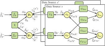
Figure 2: Factor graph representing the factorization (24) of the joint posterior pdf $f(\bm{y},\bm{a},\bm{b}|\bm{z})$ for one time step $n$. For conciseness, the indices $n$, $j$ (inner-loop iteration index), and $i$ (outer-loop iteration index) are omitted, and the following short notations are used: $\tilde{f}^{-}_{k}\!\triangleq\!\tilde{f}(\bm{y}_{n-1,k})$, $\bm{y}_{k}\!\triangleq\!\bm{y}_{n,k}$, $a_{k}\!\triangleq\!a_{n,k}^{(s)}$, $b_{m}\!\triangleq\!b_{n,m}^{(s)}$, $f_{k}\!\triangleq\!f(\bm{y}_{n,k}|\bm{y}_{n-1,k})$, $\chi\!\triangleq\!\chi\big{(}\bm{\tau}_{n},M_{n}^{(0)}\big{)}$, $\upsilon_{k}\!\triangleq$ $\upsilon^{(s)}\big{(}\bm{y}_{n,k},a_{n,k}^{(s)};\bm{z}_{n}^{(s)}\big{)}$, $\psi_{km}\!\triangleq\!\psi^{(s)}\big{(}a_{n,k}^{(s)},b_{n,m}^{(s)}\big{)}$, $\alpha_{k}\!\triangleq\!\alpha(\bm{y}_{n,k})$, $\delta_{k}\!\triangleq$ $\delta^{(i)}(\bm{y}_{n,k})$, $\varepsilon_{k}\!\triangleq\!\varepsilon^{(i)}(\bm{y}_{n,k})$, $\gamma_{k}^{(s)}\!\triangleq\!\gamma^{(s)(i)}(\bm{y}_{n,k})$, $\eta_{k}\!\triangleq\!\eta^{(s)(i)}\big{(}a_{n,k}^{(s)}\big{)}$, $\beta_{k}\!\triangleq\!\beta^{(s)(i)}\big{(}a_{n,k}^{(s)}\big{)}$, $\nu_{mk}\!\triangleq\nu_{m\rightarrow k}^{(s)(j)}\big{(}a_{n,k}^{(s)}\big{)}$, and $\xi_{km}\!\triangleq\xi_{k\rightarrow m}^{(s)(j)}\big{(}b_{n,m}^{(s)}\big{)}$.

In the next subsections, we will present expressions of the SPA messages that are passed between the various nodes of the factor graph in Fig. 2, as shown there. Some of these expressions were already provided in [26]. The expressions are obtained by direct application of the general SPA rules described in [21, 22], and are introduced in what follows in the order in which they are calculated at each time step $n$. We will denote by $I$ and $i\!\in\!\{1,\ldots,I\}$ the number of iterations and the iteration index, respectively, for the outer loop, and by $J$ and $j\!\in\!\{1,\ldots,J\}$ the number of iterations and the iteration index, respectively, for the inner loop. Furthermore, the final approximation of the marginal posterior pdf $f(\bm{y}_{n,k}|\bm{z})$is denoted by $\tilde{f}(\bm{y}_{n,k})$ and referred to as a belief.

V-A Prediction

In the prediction step, the beliefs computed at the previous time step, $\tilde{f}(\bm{y}_{n-1,k})=\tilde{f}(\bm{x}_{n-1,k},r_{n-1,k},\tau_{n-1,k})$, are propagated to the current time $n$ and converted into messages $\alpha(\bm{y}_{n,k})=\alpha(\bm{x}_{n,k},r_{n,k},\tau_{n,k})$ according to

$$\alpha(\bm{x}_{n,k},r_{n,k},\tau_{n,k})$$

$$=\!\sum_{r_{n-1,k}\in\{0,1\}}\sum_{\tau_{n-1,k}\in\mathcal{D}_{0}}\hskip 0.85358pt\int\tilde{f}(\bm{x}_{n-1,k},r_{n-1,k},\tau_{n-1,k})$$

$$\hskip 19.91692pt\times f(\bm{x}_{n,k},r_{n,k},\tau_{n,k}|\bm{x}_{n-1,k},r_{n-1,k},\tau_{n-1,k})\hskip 0.85358ptd\bm{x}_{n-1,k}$$

$$=\!\sum_{r_{n-1,k}\in\{0,1\}}\sum_{\tau_{n-1,k}\in\mathcal{D}_{0}}\!p(\tau_{n,k}|r_{n,k},r_{n-1,k},\tau_{n-1,k})$$

$$\hskip 19.91692pt\times\!\int f(\bm{x}_{n,k},r_{n,k}|\bm{x}_{n-1,k},r_{n-1,k})$$

$$\hskip 45.5244pt\times\tilde{f}(\bm{x}_{n-1,k},r_{n-1,k},\tau_{n-1,k})\hskip 0.85358ptd\bm{x}_{n-1,k}\hskip 0.85358pt,$$ (27)

where we used (3) for $f(\bm{x}_{n,k},r_{n,k},\tau_{n,k}|\bm{x}_{n-1,k},r_{n-1,k},\linebreak\tau_{n-1,k})$. As shown in Fig. 2, the messages $\alpha(\bm{x}_{n,k},r_{n,k},\tau_{n,k})$ are passed from the factor nodes “$f_{k}$” to the variable nodes “$\bm{y}_{k}$”. From (27) and the fact that $\tilde{f}(\bm{x}_{n-1,k},r_{n-1,k},\tau_{n-1,k})$ is normalized, it follows that $\alpha(\bm{x}_{n,k},r_{n,k},\tau_{n,k})$ is normalized too, i.e., $\sum_{r_{n,k}\in\{0,1\}}\sum_{\tau_{n,k}\in\mathcal{D}_{0}}\int\!\alpha(\bm{x}_{n,k},r_{n,k},\tau_{n,k})\hskip 0.85358ptd\bm{x}_{n,k}\!=\!1$. It will be convenient to introduce

$$\alpha_{n,k} \triangleq\!\sum_{\tau_{n,k}\in\mathcal{D}_{0}}\int\!\alpha(\bm{x}_{n,k},0,\tau_{n,k})\hskip 0.85358ptd\bm{x}_{n,k}$$

$$=\int\!\alpha(\bm{x}_{n,k},0,0)\hskip 0.85358ptd\bm{x}_{n,k}$$

$$=1-\!\sum_{\tau_{n,k}\in\mathcal{D}_{0}}\int\!\alpha(\bm{x}_{n,k},1,\tau_{n,k})\hskip 0.85358ptd\bm{x}_{n,k}\hskip 0.85358pt,$$ (28)

where the second step follows from (4). We note that $1\!-\alpha_{n,k}$$=\sum_{\tau_{n,k}\in\mathcal{D}_{0}}\hskip 0.85358pt\int\alpha(\bm{x}_{n,k},1,\tau_{n,k})\hskip 0.85358ptd\bm{x}_{n,k}$ can be interpreted as the predicted probability of existence of PT $k$.

V-B Outer Loop

The outer loop is composed of the factor node “$\chi$”, the variable nodes “$\bm{y}_{k}$”, and the blocks designated “Data Source” in Fig. 2; the latter process the observations provided by the TIPS sensors and the TDRS. The messages passed from “$\chi$” to “$\bm{y}_{k}$” in the $i$th outer-loop iteration are calculated as

$$\delta^{(i)}(\bm{y}_{n,k}) =\!\sum_{\bm{\tau}_{n,k}^{-}\in\mathcal{D}_{0}^{K-1}}\sum_{\bm{r}_{n,k}^{-}\in\{0,1\}^{K-1}}\!\!\chi\big{(}\bm{\tau}_{n},M_{n}^{(0)}\big{)}$$

$$\hskip 19.91692pt\times\!\!\prod_{k^{\prime}\in\mathcal{K}\setminus\{k\}}\int\varepsilon^{(i)}(\bm{y}_{n,k^{\prime}})\hskip 0.85358ptd\bm{x}_{n,k^{\prime}}$$

$$=\!\sum_{\bm{\tau}_{n,k}^{-}\in\mathcal{D}_{0}^{K-1}}\!\!\chi\big{(}\bm{\tau}_{n},M_{n}^{(0)}\big{)}\!\prod_{k^{\prime}\in\mathcal{K}\setminus\{k\}}\!\!\tilde{\varepsilon}^{(i)}(\tau_{n,k^{\prime}})\hskip 0.85358pt.$$

Here, $\bm{r}_{n,k}^{-}\!\triangleq\![r_{n,1},\ldots,r_{n,k-1},r_{n,k+1},\ldots,r_{n,K}]^{\raisebox{0.0pt}[0.0pt][0.0pt]{\scriptsize{{t}}}}$ is the vector of all the existence variables except the $k$th; $\bm{\tau}_{n,k}^{-}\!\triangleq\![\tau_{n,1},\linebreak\ldots,\tau_{n,k-1},\tau_{n,k+1},\ldots,\tau_{n,K}]^{\raisebox{0.0pt}[0.0pt][0.0pt]{\scriptsize{{t}}}}$ is the vector of all the TID variables except the $k$th; $\varepsilon^{(i)}(\bm{y}_{n,k})$ are the messages passed from “$\bm{y}_{k}$” to “$\chi$”, which are calculated as

$$\varepsilon^{(i)}(\bm{y}_{n,k})=\alpha(\bm{y}_{n,k})\prod_{s=0}^{S}\gamma^{(s)(i)}(\bm{y}_{n,k})\hskip 0.85358pt;$$ (30)

and

$$\tilde{\varepsilon}^{(i)}(\tau_{n,k})\triangleq\!\sum_{r_{n,k}\in\{0,1\}}\int\!\varepsilon^{(i)}(\bm{x}_{n,k},r_{n,k},\tau_{n,k})\hskip 0.85358ptd\bm{x}_{n,k}\hskip 0.85358pt.$$ (31)

The messages $\gamma^{(s)(i)}(\bm{y}_{n,k})$ in (30), which are passed from the data source blocks to “$\bm{y}_{k}$”, will be presented in Section V-D. We finally note that, according to expression (LABEL:eq:delta_k), $\delta^{(i)}(\bm{y}_{n,k})$ depends only on $\tau_{n,k}$. Thus, we will denote it as $\tilde{\delta}^{(i)}(\tau_{n,k})$.

V-C Observation Evaluation

A further operation within the $i$th outer-loop iteration is the calculation of the messages

$$\beta^{(s)(i)}\big{(}a_{n,k}^{(s)}\big{)} =\!\!\!\sum_{\tau_{n,k}\in\mathcal{D}_{0}}\!\!\!\tilde{\delta}^{(i-1)}(\tau_{n,k})\!\!\!\!\!\sum_{r_{n,k}\in\{0,1\}}\int\!\alpha(\bm{x}_{n,k},r_{n,k},\tau_{n,k})$$

$$\hskip 9.95845pt\times\upsilon^{(s)}\big{(}\bm{x}_{n,k},r_{n,k},\tau_{n,k},a_{n,k}^{(s)};\bm{z}_{n}^{(s)}\big{)}\hskip 0.85358ptd\bm{x}_{n,k}$$ (32)

for all PTs $k\!\in\!\mathcal{K}$ and data sources $s\!\in\!\mathcal{S}_{0}$, with $\tilde{\delta}^{(0)}(\tau_{n,k})=1$. These messages are passed from the factor nodes “$\upsilon_{k}$” to the variable nodes “$a_{k}$”. Differently from the previously presented messages, $\beta^{(s)(i)}\big{(}a_{n,k}^{(s)}\big{)}$ involves the observation $\bm{z}_{n}^{(s)}$. Let us introduce the shorthand $\beta^{(s)(i)}_{n,k}(m)\triangleq\beta^{(s)(i)}\big{(}a_{n,k}^{(s)}\!=\!m\big{)}$. Then, for the TDRS, i.e., $s\!=\!0$, using (26) and the definitions of the functions $h^{(0)}\big{(}\bm{x}_{n,k},r_{n,k},\tau_{n,k},a_{n,k}^{(0)};M_{n}^{(0)}\big{)}$ and $g^{(0)}\big{(}\bm{x}_{n,k},\linebreak r_{n,k},\tau_{n,k},a_{n,k}^{(0)};\bm{z}_{n}^{(0)}\big{)}$ introduced in Section III-D and Section III-E, respectively, we obtain for all $m\!\in\!\mathcal{M}_{n}^{(0)}$

$$\beta^{(0)(i)}_{n,k}(m) =\!\sum_{\tau_{n,k}\in\mathcal{D}}\!\tilde{\delta}^{(i-1)}(\tau_{n,k})\,p(\zeta_{n,m}|\tau_{n,k})$$

$$\hskip 14.22636pt\times\!\int\!f(\bm{q}_{n,m}|\bm{x}_{n,k})\hskip 0.85358pt\alpha(\bm{x}_{n,k},1,\tau_{n,k})\hskip 0.85358ptd\bm{x}_{n,k}\hskip 0.85358pt,$$ (33)

and for $m\!=\!0$

$$\beta^{(0)(i)}_{n,k}(0) =\!\sum_{\tau_{n,k}\in\mathcal{D}_{0}}\!\!\tilde{\delta}^{(i-1)}(\tau_{n,k})$$

$$\hskip 14.22636pt\times\!\Big{(}\alpha_{n,k}\hskip 0.85358pt\mathds{1}(\tau_{n,k})+\!\int\!\alpha(\bm{x}_{n,k},1,\tau_{n,k})\hskip 0.85358ptd\bm{x}_{n,k}\Big{)}\hskip 0.85358pt,$$ (34)

where definition (28) has been used. For the TIPS sensors $s\!\in\!\mathcal{S}$, expression (32) specializes as follows:

$$\beta^{(s)(i)}\big{(}a_{n,k}^{(s)}\big{)} =\tilde{\delta}^{(i-1)}(\tau_{n,k}\!=0)\hskip 0.85358pt\alpha_{n,k}\hskip 0.85358pt\mathds{1}\big{(}a_{n,k}^{(s)}\big{)}\hskip 0.85358pt$$

$$\hskip 11.38109pt+\!\sum_{\tau_{n,k}\in\mathcal{D}_{0}}\!\!\tilde{\delta}^{(i-1)}(\tau_{n,k})\!\int\!\alpha(\bm{x}_{n,k},1,\tau_{n,k})$$

$$\hskip 21.33955pt\times\upsilon^{(s)}\big{(}\bm{x}_{n,k},1,\tau_{n,k},a_{n,k}^{(s)};\bm{z}_{n}^{(s)}\big{)}\hskip 0.85358ptd\bm{x}_{n,k}\hskip 0.85358pt.$$ (35)

The messages $\beta^{(s)(i)}\big{(}a_{n,k}^{(s)}\big{)}$ are used for the iterative probabilistic data association algorithm discussed next.

V-D Inner Loop: Iterative Probabilistic Data Association

Iterative probabilistic data association corresponds to passing messages $\nu_{m\rightarrow k}^{(s)(j)}\big{(}a_{n,k}^{(s)}\big{)}$ and $\xi_{k\rightarrow m}^{(s)(j)}\big{(}b_{n,m}^{(s)}\big{)}$ on the inner loop. In the $j$th inner-loop iteration, following [30], these messages are calculated for each PT $k\!\in\!\mathcal{K}$, data source $s\!\in\!\mathcal{S}_{0}$, and observation $m\!\in\!\mathcal{M}_{n}^{(s)}$ according to

$$\xi_{k\rightarrow m}^{(s)(j)}\big{(}b_{n,m}^{(s)}\big{)} =\!\sum_{a_{n,k}^{(s)}=0}^{M_{n}^{(s)}}\!\!\psi^{(s)}\big{(}a_{n,k}^{(s)},b_{n,m}^{(s)}\big{)}\hskip 0.85358pt\beta^{(s)(i)}\big{(}a_{n,k}^{(s)}\big{)}$$

$$\hskip 19.91692pt\times\!\!\prod_{m^{\prime}\in\mathcal{M}_{n}^{(s)}\setminus\{m\}}\!\!\!\nu_{m^{\prime}\rightarrow k}^{(s)(j-1)}\big{(}a_{n,k}^{(s)}\big{)}$$ (36)

and

$$\nu_{m\rightarrow k}^{(s)(j)}\big{(}a_{n,k}^{(s)}\big{)} =\!\sum_{b_{n,m}^{(s)}=0}^{K}\!\!\psi^{(s)}\big{(}a_{n,k}^{(s)},b_{n,m}^{(s)}\big{)}\!\prod_{k^{\prime}\in\mathcal{K}\setminus\{k\}}\!\!\!\xi_{k^{\prime}\!\rightarrow m}^{(s)(j)}\big{(}b_{n,m}^{(s)}\big{)}\hskip 0.85358pt.$$

(We note that these messages also depend on the outer-loop iteration index $i$, which is omitted to simplify the notation.) The iteration constituted by (36) and (LABEL:eq:nu_full) is initialized by $\nu_{m\rightarrow k}^{(s)(0)}\big{(}a_{n,k}^{(s)}\big{)}\!=\!1$. After all the inner-loop iterations $j=1,\ldots,J$ have been performed, the messages $\nu_{m\rightarrow k}^{(s)(J)}\big{(}a_{n,k}^{(s)}\big{)}$ are available. These messages are then used to calculate messages $\eta^{(s)(i)}\big{(}a_{n,k}^{(s)}\big{)}$, which are passed from variable nodes “$a_{k}$” back to factor nodes “$\upsilon_{k}$”, according to

$$\eta^{(s)(i)}\big{(}a_{n,k}^{(s)}\big{)}=\!\prod_{m\in\mathcal{M}_{n}^{(s)}}\!\!\nu_{m\rightarrow k}^{(s)(J)}\big{(}a_{n,k}^{(s)}\big{)}\hskip 0.85358pt.$$ (38)

Finally, messages $\gamma^{(s)(i)}(\bm{y}_{n,k})$, which are passed from factor nodes “$\upsilon_{k}$” to variable nodes “$\bm{y}_{k}$”, are calculated as

$$\hskip 0.85358pt\gamma^{(s)(i)}(\bm{y}_{n,k})=\!\sum_{a_{n,k}^{(s)}=0}^{M_{n}^{(s)}}\!\!\upsilon^{(s)}\big{(}\bm{y}_{n,k},a_{n,k}^{(s)};\bm{z}_{n}^{(s)}\big{)}\hskip 0.85358pt\eta^{(s)(i)}\big{(}a_{n,k}^{(s)}\big{)}\hskip 0.85358pt.\!\!\!\!$$ (39)

Following [30] with certain modifications, an efficient implementation of the above algorithm with a complexity of $O(KM_{n}^{(s)})$ per inner-loop iteration can be developed. This implementation is based on the fact that, due to the definition of the binary function $\psi^{(s)}\big{(}a_{n,k}^{(s)},b_{n,m}^{(s)}\big{)}$ in Section III-C, the expressions (36) and (LABEL:eq:nu_full) can take on only two different values. A detailed derivation and formulation is provided in the supplementary material manuscript [29].

V-E Belief Calculation

After all the outer-loop iterations $i=1,\ldots,I$ have been performed, the messages $\tilde{\delta}^{(I)}(\tau_{n,k})$ and $\gamma^{(s)(I)}(\bm{y}_{n,k})$ are available. The final step is to calculate the beliefs $\tilde{f}(\bm{x}_{n,k},\linebreak r_{n,k},\tau_{n,k})$ approximating the marginal posterior pdfs $f(\bm{x}_{n,k},\linebreak r_{n,k},\tau_{n,k}|\bm{z})$ as

$$\tilde{f}(\bm{x}_{n,k},r_{n,k},\tau_{n,k}) =\frac{1}{C_{n,k}}\hskip 0.85358pt\alpha(\bm{x}_{n,k},r_{n,k},\tau_{n,k})\hskip 0.85358pt\tilde{\delta}^{(I)}(\tau_{n,k})$$

$$\hskip 14.22636pt\times\prod_{s=0}^{S}\gamma^{(s)(I)}(\bm{x}_{n,k},r_{n,k},\tau_{n,k})\hskip 0.85358pt,$$ (40)

with $C_{n,k}\triangleq\sum_{r_{n,k}\in\{0,1\}}\sum_{\tau_{n,k}\in\mathcal{D}_{0}}\int\tilde{f}(\bm{x}_{n,k},r_{n,k},\tau_{n,k})\hskip 0.85358ptd\bm{x}_{n,k}$.

V-F Implementation and Complexity Reduction

Algorithm 1 SPA-Based MTT Algorithm with TIPS-TDRS Fusion

1:$\tilde{f}(\bm{y}_{n-1,k})$, $\bm{z}_{n}$.

2:$\tilde{f}(\bm{y}_{n,k})$

3:Prediction   Compute $\alpha(\bm{y}_{n,k})$ for all $k\!\in\!\mathcal{K}$ as in (27)

4:Outer Loop

5:$\delta^{(0)}(\bm{y}_{n,k})\longleftarrow 1$

6:for $i=1$ to $I$ do

7:Observation Evaluation

8:     for $s=0$ to $S$ do (in parallel)

9:         Compute $\beta^{(s)(i)}(a_{n,k}^{(s)})$ for all $k\!\in\!\mathcal{K}$ as in (32)

10:         Inner Loop   Compute data association messages (36) and (LABEL:eq:nu_full)

11:         Compute $\eta^{(s)(i)}(a_{n,k}^{(s)})$ for all $k\!\in\!\mathcal{K}$ as in (38)

12:         Compute $\gamma^{(s)(i)}(\bm{y}_{n,k})$ for all $k\!\in\!\mathcal{K}$ as in (39)

13:     end for

14:     Compute $\varepsilon^{(i)}(\bm{y}_{n,k})$ for all $k\!\in\!\mathcal{K}$ as in (30)

15:     Compute $\delta^{(i)}(\bm{y}_{n,k})$ for all $k\!\in\!\mathcal{K}$ as in (LABEL:eq:delta_k)

16:end for

17:Belief Computation   Compute $\tilde{f}(\bm{y}_{n,k})$ for all $k\!\in\!\mathcal{K}$ as in (40)

A step-by-step summary of the proposed SPA-based MTT algorithm with TIPS-TDRS fusion is provided in Algorithm 1. A particle-based implementation can be obtained by extending the algorithm presented in [18]. This implementation approximates the beliefs $\tilde{f}(\bm{y}_{n,k})$ as well as the messages $\alpha(\bm{y}_{n,k})$ and $\gamma^{(s)(i)}(\bm{y}_{n,k})$ by a set of particles and corresponding weights [32], thereby avoiding the direct computation of integrals and enabling a feasible computation of the messages and beliefs.

However, the computation of the message $\tilde{\delta}^{(i)}(\tau_{n,k})$ can still be expensive; indeed, according to (LABEL:eq:delta_k), $\tilde{\delta}^{(i)}(\tau_{n,k})$ is the sum of $(D+1)^{K-1}$ terms, and thus its computation scales exponentially in the number $K$ of PTs. We therefore propose a low-complexity (LC) computation in which $\tilde{\delta}^{(i)}(\tau_{n,k})$ is approximated with only a single term, given by

$$\tilde{\delta}^{(i)}(\tau_{n,k})\approx\chi\big{(}\bm{\tau}_{n}^{\star},M_{n}^{(0)}\big{)}\!\prod_{k^{\prime}\in\mathcal{K}\setminus\{k\}}\!\!\tilde{\varepsilon}^{(i)}(\tau_{n,k^{\prime}}^{\star})\hskip 0.85358pt,\vspace{-1mm}$$ (41)

where $\bm{\tau}_{n}^{\star}\triangleq[\tau_{n,1}^{\star},\ldots,\tau_{n,k-1}^{\star},\tau_{n,k},\tau_{n,k+1}^{\star},\ldots,\tau_{n,K}^{\star}]^{\raisebox{0.0pt}[0.0pt][0.0pt]{\scriptsize{{t}}}}$ and $\tau_{n,k}^{\star}\triangleq\operatorname*{arg\,max}_{\,\tau_{n,k}\in\mathcal{D}_{0}}\tilde{\varepsilon}^{(i)}(\tau_{n,k})$. To motivate (41), we note that at each step of the outer loop, $\tilde{\varepsilon}^{(i)}(\tau_{n,k})$ can be interpreted as the (nonnormalized) probability distribution of $\tau_{n,k}$, the TID of PT $k$, after observation evaluation and data association. The messages $\tilde{\varepsilon}^{(i)}(\tau_{n,k^{\prime}})$ coming from all PTs $k^{\prime}\!\not=k$ are then used to obtain $\tilde{\delta}^{(i)}(\tau_{n,k})$. More specifically, according to the summation in (LABEL:eq:delta_k), all the possible combinations between the TIDs in $\mathcal{D}_{0}$ and the PTs (except the $k$th) are evaluated and weighted by $\chi(\bm{\tau}_{n},M_{n}^{(0)})$, and the corresponding terms are marginalized out. The LC approximation (41) then corresponds to considering only the most likely of these combinations. In Section VI, we will verify experimentally the validity of this approximation.

VI Results for Simulated Data

We evaluate the performance of the proposed MTT algorithm with TIPS-TDRS fusion in a simulated scenario, and we compare it with that of three alternative algorithms.

VI-A Experiment Setup

The simulated scenario consists of nine targets that are moving in a region of interest (ROI) with a constant velocity of $4$ m/s during 200 time steps, with time step duration $T\!=\!10\,\text{s}$.The target trajectories, whose starting points are equally spaced on a circle with center $(0,0)$ and radius $4$ km, and the ROI are shown in Fig. 3. Five targets appear at $n\!=\!1$ and disappear at $n\!=\!200$, and the other four targets appear at $n\!=\!5$ and disappear at $n\!=\!195$. Six randomly selected targets are cooperative and transmit TDRS reports between $n\!=\!10$ and $n\!=\!190$; the number of TDRS reports transmitted per time interval is a random variable that is Poisson distributed with mean $0.5$ for three of the six cooperative targets and $2$ for the other three cooperative targets.

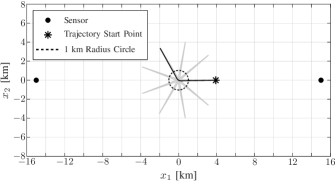
Figure 3: Simulated scenario: TIPS sensors (black bullets) and target trajectories. The star marks the initial position of the highlighted trajectory; the other trajectories are rotated (by $40$ degrees) versions of the former.

The PT states $\bm{x}_{n,k}$ are composed of the 2D position vector $\check{\bm{x}}_{n,k}$ and the 2D velocity vector $\dot{\check{\bm{x}}}_{n,k}$, i.e., $\bm{x}_{n,k}\!=\![\check{\bm{x}}_{n,k}^{\raisebox{0.0pt}[0.0pt][0.0pt]{\scriptsize{{t}}}},\dot{\check{\bm{x}}}_{n,k}^{\raisebox{0.0pt}[0.0pt][0.0pt]{\scriptsize{{t}}}}]^{\raisebox{0.0pt}[0.0pt][0.0pt]{\scriptsize{{t}}}}\!$. For the dynamic model in (1), we choose the nearly constant velocity model, i.e., $\bm{x}_{n,k}\!=\!\bm{F}\bm{x}_{n-1,k}+\bm{G}\bm{u}_{n,k}$, where $\bm{F}\!\in\!\mathbb{R}^{4\times 4}$ and $\bm{G}\!\in\!\mathbb{R}^{4\times 2}$ are defined as in [33, Sec. 6.3.2] (this involves the time step duration $T$) and $\bm{u}_{n,k}\!\sim\!\mathcal{N}(\bm{0},\sigma_{\text{u}}^{2}{\bf I}_{2})$ is a 2D zero-mean iid Gaussian random vector that is also iid across $n$ and $k$, with $\sigma_{\text{u}}\!=\!0.05$ m/s².

There are two TIPS sensors (i.e., $S\!=\!2$), which generate range-bearing measurements $\bm{z}_{n,m}^{(s)}\!=\!\big{[}z_{n,m,\text{r}}^{(s)}\hskip 0.85358pt,z_{n,m,\text{b}}^{(s)}\big{]}^{\raisebox{0.0pt}[0.0pt][0.0pt]{\scriptsize{{t}}}}$, $s\!\in\!\mathcal{S}$. The range measurement $z_{n,m,\text{r}}^{(s)}$ is a Gaussian random variable with mean $\left\|\check{\bm{x}}_{n,k}\!-\bm{\rho}^{(s)}\right\|$ and standard deviation $\sigma_{\text{r}}^{(s)}\!=\!\sigma_{\text{r}}\!=\!250$ m, and the bearing measurement $z_{n,m,\text{b}}^{(s)}$ is a von Mises random variable with mean $\angle(\check{\bm{x}}_{n,k}-\bm{\rho}^{(s)})$ and concentration parameter $\kappa_{\text{b}}^{(s)}\!=\!\kappa_{\text{b}}=500$ [34, Ch. 3.5.4]. Here, $\bm{\rho}^{(1)}\!=\![15,0]^{\raisebox{0.0pt}[0.0pt][0.0pt]{\scriptsize{{t}}}}$ km and $\bm{\rho}^{(2)}\!=\![-15,0]^{\raisebox{0.0pt}[0.0pt][0.0pt]{\scriptsize{{t}}}}$ km are the positions of the TIPS sensors. Furthermore, the mean number of false alarms is $\mu^{(s)}\!=\!2$ and the false alarm pdf $f_{\text{FA}}(\bm{z}_{n,m}^{(s)})$ is uniform on the ROI and zero outside. The detection probability is $P_{\text{d}}^{(s)}(\bm{x}_{n,k})\!=\!P_{\text{d}}^{(s)}\!=\!0.5$.

The TDRS self-measurement is modeled as $\bm{q}_{n,m}^{(\ell)}\!=\check{\bm{x}}_{n,k,m}^{(\ell)}+\bm{v}_{n,m}^{(\ell)}$, where $\bm{v}_{n,m}^{(\ell)}\!\sim\!\mathcal{N}(\bm{0},\sigma_{\text{v}}^{2}{\bf I}_{2})$ with $\sigma_{\text{v}}=10\,$m is a 2D zero-mean iid Gaussian random vector that is also iid across $n$, $m$, and $\ell$. The ID set is chosen as $\mathcal{D}\!=\!\{1,2,\ldots,6\}$. The probability that the PT-to-TDRS transmission is successful and without errors is $p_{n,m}^{\text{c}}\!=\!p^{\text{c}}\!=\!0.95$, and the probability that there is an error resulting in an RID outside $\mathcal{D}$ is $p_{n,m}^{\text{e}}\!=\!p^{\text{e}}\!=\!0.045$; the RIDs within the reports are simulated in accordance with these probabilities. Finally, each TDRS report time $t_{n,m}^{(\ell)}$ is randomly (uniformly) chosen within the respective time step interval $(t_{n-1},t_{n}]$.

We compare our algorithm, which jointly processes TIPS and TDRS observations at each time step $n$, with three alternative algorithms. The first conforms to the system model proposed in Section III except that the TDRS reports are sequentially processed as soon as they become available and, thus, the PT states are estimated each time a TDRS report is received; this will thus be called the “sequential” algorithm. The second alternative algorithm, which we will refer to as the “all-TIPS” algorithm, models and treats the TDRS as a TIPS sensor. Accordingly, the TDRS clusters are considered as TIPS measurements, which means that their RID is ignored (once the clusters are formed) and the possibility that they are false alarms is not ruled out. For this virtual TIPS sensor, we assume a detection probability of $P_{\text{d}}^{(0)}\!=\!0.9$, $0.5$, or $0.25$—depending on the scenario—and a mean number of false alarms of $\mu^{(0)}\!=\!10^{-16}$. Here, the small value of $\mu^{(0)}$ reflects the low mean number of false alarms expected from the TDRS. (We do not set $\mu^{(0)}$ to $0$, because this would result in a division by $0$ in the expression of $h^{(s)}(\cdot)$ reported below equation (15).) The third alternative algorithm is the one proposed in [18], which fuses only the TIPS measurements and will hence be called the “no-TDRS” algorithm. We use the following parameters in all algorithms if applicable and unless otherwise stated: $K=30$, $p^{\text{t}}_{n,k}\!=\!p^{\text{t}}\!=\!0.1$, $p^{\text{b}}_{n,k}\!=\!p^{\text{b}}\!=\!10^{-3}$, $p^{\text{s}}_{n,k}\!=\!p^{\text{s}}\!=\!0.999$, and $P_{\text{th}}=0.95$.

We assess the performance of the various algorithms in terms of the Euclidean distance based generalized optimal sub-pattern assignment error for trajectories (GOSPA-T) [35], with cut-off parameter $c=500\,$m, switching penalty 250 m, and order 1. The GOSPA-T metric accounts for localization errors for correctly confirmed targets, errors for missed targets and false targets (i.e., confirmed PTs not corresponding to any actual target), and an error for track switches. Furthermore, we report the time on target (ToT), track fragmentation (TF), and false alarm rate (FAR). The ToT is the fraction of time during which the PT corresponding to a target is confirmed and the distance between its estimated and true positions is lower than 500 m. The TF is the number of different PTs associated with a target during the target’s lifespan. The FAR is the number of false tracks per unit of space and unit of time. As the ToT and TF are defined for each target individually, we will usually consider their averages taken over all targets, which will be referred to as A-ToT and A-TF, respectively. Finally, to evaluate the accuracy in estimating the TIDs for the proposed algorithm and the sequential algorithm, we report a metric referred to as the TID errors count. At each time step $n$, given the optimal sub-pattern assignment (with cut-off parameter $c=500\,$m) between the actual targets and the estimated PTs, the TID errors count is defined as the number of errors committed by the tracking algorithm in estimating all the TIDs. All the mentioned performance indices are averaged over 100 simulation runs.

VI-B Effect of the LC Approximation

We first assess the validity of the LC approximation (41) by comparing the resulting performance with that of the full-complexity (FC) computation of the messages $\tilde{\delta}^{(i)}(\tau_{n,k})$ according to (LABEL:eq:delta_k). To avoid an excessive complexity of the FC computation, we temporarily consider only three targets—two cooperative and one noncooperative—and choose $K\!=\!10$ and $\mathcal{D}\!=\!\{1,2\}$. Fig. 4 shows the mean GOSPA-T of the LC and FC versions versus time step $n$. One can see that the LC approximation does not reduce the performance of the proposed algorithm. This is confirmed by Fig. 5, which shows the mean TID errors count, and by Fig. 6, which shows the A-ToT versus FAR performance for varying existence confirmation threshold $P_{\text{th}}$ (cf. Section IV). A further confirmation is provided by the fact that the A-TF was obtained as $1.34$ for the FC version and $1.35$ for the LC version.

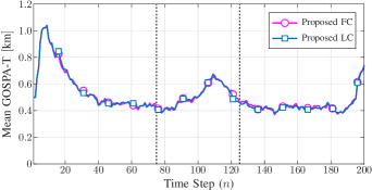
Figure 4: Mean GOSPA-T obtained with the proposed algorithm using the FC and LC implementations of the outer loop. In this figure and in subsequent figures, the dashed vertical lines delimit the time interval during which the targets are within the circle of radius 1 km shown in Fig. 3.

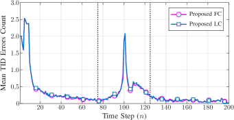
Figure 5: Mean TID errors count obtained with the proposed algorithm using the FC and LC implementations of the outer loop.

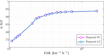
Figure 6: A-ToT versus FAR obtained for varying existence confirmation threshold $P_{\text{th}}$ using the FC and LC implementations of the outer loop.

VI-C Comparison with Alternative Algorithms

Fig. 7 compares the mean GOSPA-T of the proposed algorithm (with LC approximation), of the all-TIPS algorithm with $P_{\text{d}}^{(0)}\!\!=\!0.9$, $P_{\text{d}}^{(0)}\!\!=\!0.5$, and $P_{\text{d}}^{(0)}\!\!=\!0.25$, of the sequential algorithm, and of the no-TDRS algorithm. The proposed algorithm is seen to consistently outperform both the all-TIPS algorithm, independently of the chosen detection probability $P_{\text{d}}^{(0)}$, and the no-TDRS algorithm. The performance difference between the proposed algorithm and the all-TIPS algorithm is largest in the time interval between time steps $n\!=\!75$ and $n\!=\!125$, when the targets are within the circle of radius 1 km shown in Fig. 3 and perform a smooth right turn. Indeed, the exploitation of the RID included in the TDRS reports enables the proposed algorithm to accurately track the targets even while maneuvering. The performance of the proposed algorithm and the sequential algorithm is quite similar, with a slightly higher mean GOSPA-T obtained with the proposed algorithm. This is arguably due to the immediate processing of the TDRS reports performed by the sequential algorithm: because the TDRS reports are processed as soon as they are received, the PT state prediction is performed over a shorter time interval, which reduces the growth of uncertainty over time. On the other hand, as shown next, the sequential processing leads to an inaccurate estimation of the TIDs.

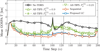
Figure 7: Mean GOSPA-T obtained with the proposed algorithm (with LC approximation) and with the sequential, all-TIPS, and no-TDRS algorithms.

Fig. 8 presents a comparison between the proposed algorithm and the sequential algorithm in terms of the mean TID errors count. It can be seen that the mean TID errors count of the sequential algorithm is consistently higher than that of the proposed algorithm, which indicates frequent errors in estimating the TIDs. At time $n\!=\!1$, the mean TID errors count is equal to 5 because only five targets are present in the ROI; it then increases at time $n\!=\!5$ when the other four targets appear. The peak at time $n\!=\!100$ is mostly due to an erroneous assignment between the PTs and the actual targets, which is due to the close proximity of all the targets.

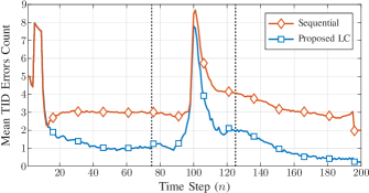
Figure 8: Mean TID errors count obtained with the proposed algorithm (with LC approximation) and the sequential algorithm.

Fig. 9 compares the A-ToT versus FAR performance of the proposed algorithm and the three alternative algorithms. It is seen that the proposed algorithm outperforms the other algorithms in that it yields the highest A-ToT for a given FAR.

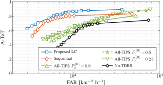
Figure 9: A-ToT versus FAR performance of the proposed algorithm (with LC approximation) and of the sequential, all-TIPS, and no-TDRS algorithms.

Finally, the proposed algorithm outperforms the other algorithms also in terms of the A-TF. Indeed, we obtained its A-TF as $2.45$, which is lower than the A-TF of the all-TIPS algorithm ($4.81$, $3.93$, and $3.67$ for $P_{\text{d}}^{(0)}\!=\!0.9$, $0.5$, and $0.25$, respectively), of the sequential algorithm ($2.62$), and of the no-TDRS algorithm ($3.64$).

VII Results for Real Data

Next, we apply the proposed algorithm to a real dataset acquired in a maritime scenario and compare its results with those obtained with the sequential algorithm. The dataset has a duration of about 7.5 hours and consists of TIPS measurements provided by two radar sensors (i.e., $S\!=\!2$) and TDRS reports provided by the AIS. The radar measurements were acquired by two high-frequency surface wave (HFSW) radars [36] located on the Italian coast, one on the island of Palmaria (IP) near La Spezia and the other in San Rossore Park (SRP) near Pisa. Each measurement consists of range, bearing, and range rate, i.e., $\bm{z}_{n,m}^{(s)}\!=\!\big{[}z_{n,m,\text{r}}^{(s)},z_{n,m,\text{b}}^{(s)},z_{n,m,\dot{\text{r}}}^{(s)}\big{]}^{\raisebox{0.0pt}[0.0pt][0.0pt]{\scriptsize{{t}}}}$. The range measurement $z_{n,m,\text{r}}^{(s)}$ and bearing measurement $z_{n,m,\text{b}}^{(s)}$ are modeled as described in Section VI-A, with $\sigma_{\text{r}}\!=\!150$ m and $\kappa_{\text{b}}\!=\!1000$. The range rate measurement is modeled as a Gaussian random variable with mean $(\check{\bm{x}}_{n,k}-\bm{\rho}^{(s)})^{\raisebox{0.0pt}[0.0pt][0.0pt]{\scriptsize{{t}}}}\hskip 0.85358pt\dot{\check{\bm{x}}}_{n,k}/\left\|\check{\bm{x}}_{n,k}\!-\bm{\rho}^{(s)}\right\|$ and standard deviation $\sigma_{\dot{\text{r}}}^{(s)}\!=\!\sigma_{\dot{\text{r}}}\!=\!0.1$ m$/$s. The mean number of false alarms is set to $\mu^{(s)}\!=\!15$, and the false alarm pdf $f_{\text{FA}}(\bm{z}_{n,m}^{(s)})$ is uniform on the ROI (which is the intersection of the fields of view of the two radar sensors) and zero outside, as well as uniform in range rate in the interval $[-25,25]$ m$/$s and zero outside. The detection probability is set to $P_{\text{d}}^{(s)}\!=0.8$.

Each AIS report contains an RID, i.e., the maritime mobile service identity (MMSI), and a self-measurement of the position of the respective target (ship). The self-measurement is modeled as in Section VI-A, with $\sigma_{\text{v}}\!=\!100$ m. Due to the lack of other information sources, the AIS data are also used as ground truth for evaluating the time-averaged mean GOSPA-T and the time-averaged mean TID errors count, as well as the A-ToT, A-TF, and FAR. More specifically, a sequence of reports with the same MMSI forms an “AIS track,” which is considered to be a ground-truth trajectory. Since these AIS tracks represent only a subset of the ships actually present in the ROI, our performance assessment and comparison of the proposed algorithm and the sequential algorithm are not exhaustive; they are merely intended to demonstrate the applicability of the proposed statistical formulation and tracking algorithms to a real-world scenario. To account for the facts that the AIS sequences are not temporally aligned with the radar time steps and some of them contain “gaps” of several minutes or even hours, we use cubic interpolation to determine the instantaneous positions of the AIS tracks at each radar time step.

The number of PTs is set to $K\!=\!100$. The PT state and dynamic model are defined as in Section VI-A, with $\sigma_{\text{u}}\!=\!0.05$ m/s² and $T\!=\!16.64$ s. The existence confirmation threshold is set to $P_{\text{th}}\!=0.99$. All the other parameters involved in our algorithm are chosen as specified in Section VI-A.

In Fig. 10, we depict the measurements of the two radar sensors and the trajectories estimated by the proposed algorithm during 7.5 hours. (The trajectories estimated by the sequential algorithm are very similar; they are not shown to avoid a cluttered figure.) One can see that fusing the TIPS measurements provided by the HFSW radars and the TDRS reports provided by the AIS allows MMSI-based identification of the cooperative ships.

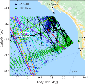
Figure 10: Measurements produced by the IP and SRP radar sensors (represented by blue and green dots, respectively) and trajectories estimated by the proposed algorithm (represented by black or colored lines) during 7.5 hours. Colored lines represent the estimated trajectories of cooperative ships identified through the MMSI, whereas black lines represent the estimated trajectories of noncooperative ships. For improved clarity, trajectories of duration less than ten time steps are not shown. The dashed white rectangle identifies the subregion depicted in Fig. 11.

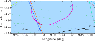
(a) Proposed algorithm.

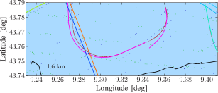
(b) Sequential algorithm.

Figure 11: Trajectories estimated by (a) the proposed algorithm and (b) the sequential algorithm in a rectangular subregion of the ROI. Blue and green dots represent measurements produced by the IP and SRP radar sensors, respectively, and red dots represent the positions indicated by the AIS reports.

On the other hand, the lack of AIS reports for the remaining noncooperative ships does not impede their tracking. Note that the superposition of the measurements seems to form line segments along some range directions of the radar sensors; these line segments are caused by a nonuniform distribution of false detections affecting HFSW radars, and do not correspond to actual ship trajectories.

Fig. 11 compares the trajectories estimated by the proposed algorithm and the sequential algorithm in a rectangular subregion of the ROI where one of the ships is maneuvering. We observe that in this specific example the proposed algorithm produces a single track for the maneuvering ship, whereas the sequential algorithm does not achieve track continuity.

The time-averaged mean GOSPA-T is $2353$ m for the proposed algorithm and $2042$ m for the sequential algorithm. These results conform to those we obtained for simulated data in Section VI-C. The time-averaged mean TID errors count is $0.05$ for the proposed algorithm and $0.78$ for the sequential algorithm, which confirms that the proposed algorithm is more accurate in estimating the TIDs. Furthermore, compared to the sequential algorithm, the proposed algorithm exhibits a higher A-ToT ($0.99$ versus $0.82$), a higher FAR ($0.14$ versus $0.12$ km^-1h^-1), and a higher A-TF ($1.31$ versus $1.23$). Note that definite conclusions cannot be drawn from these results because the ground truth is available only for a subset of the ships, i.e., for those providing AIS reports. Indeed, the results are mainly intended to demonstrate the applicability of the proposed statistical formulation and tracking algorithms to a real-world scenario.

VIII Conclusion

Heterogeneous data fusion is an important functionality in high-performance multitarget tracking (MTT) systems. In this paper, we considered multisensor MTT with an inherent probabilistic fusion of two classes of data sources: sensors that produce measurements without requiring target cooperation, and a reporting system that conveys information—possibly including target ID—that is provided by cooperative targets. We established a statistical observation model that combines these two classes of data sources and accounts for measurement-origin uncertainty, missed detections, false alarms, incorrectly received IDs, and asynchronicity.

Adopting a Bayesian framework, target existence confirmation and state estimation essentially amount to marginalizing a joint posterior distribution that involves the target states, existence indicators, and IDs, the observation-target association indices, and the past and current observations from all the sensors and the reporting system. To obtain an efficient and scalable sequential algorithm for approximate marginalization that exploits conditional independencies, we used the sum-product algorithm on a factor graph that represents the structure of our Bayesian statistical model for the multisensor MTT and information fusion problem. The resulting MTT algorithm allows a real-time integration of the two classes of data sources and exhibits high tracking accuracy at moderate complexity. We demonstrated the performance of the algorithm and the effectiveness of our fusion approach using both simulated data and real data from a maritime surveillance experiment. Our results showed the benefits of fusing heterogeneous information and substantial performance advantages over three alternative algorithms.

A possible direction of future research is the extension of the proposed framework to an indoor simultaneous localization and mapping scenario [37] enhanced by radio-frequency identification tags [38].

References

- [1] R. Mahler, Statistical Multisource-Multitarget Information Fusion. Norwood, MA, USA: Artech House, 2007.
- [2] M. Liggins, D. Hall, and J. Llinas, Handbook of Multisensor Data Fusion: Theory and Practice, 2nd ed. Boca Raton, FL, USA: Taylor & Francis, 2008.
- [3] Y. Bar-Shalom, P. K. Willett, and X. Tian, Tracking and Data Fusion: A Handbook of Algorithms. Storrs, CT, USA: YBS Publising, 2011.
- [4] W. Koch, Tracking and Sensor Data Fusion: Methodological Framework and Selected Applications. Heidelberg, Germany: Springer, 2013.
- [5] M. Mallick, B. N. Vo, T. Kirubarajan, and S. Arulampalam, “Introduction to the issue on multitarget tracking,” IEEE J. Sel. Topics Signal Process., vol. 7, no. 3, pp. 373–375, Jun. 2013.
- [6] B.-N. Vo, M. Mallick, Y. Bar-Shalom, S. Coraluppi, R. Osborne III, R. Mahler, and B.-T. Vo, “Multitarget tracking,” in Wiley Encyclopedia of Electrical and Electronics Engineering. Hoboken, NJ, USA: Wiley, 2015.
- [7] J. Petersen, Handbook of Surveillance Technologies, 3rd ed. Boca Raton, FL, USA: Taylor & Francis, 2012.
- [8] B. J. Tetreault, “Use of the automatic identification system (AIS) for maritime domain awareness (MDA),” in Proc. OCEANS-05, vol. 2, Washington, DC, USA, Sep. 2005, pp. 1590–1594.
- [9] M. Strohmeier, M. Schafer, V. Lenders, and I. Martinovic, “Realities and challenges of NextGen air traffic management: The case of ADS-B,” IEEE Commun. Mag., vol. 52, no. 5, pp. 111–118, May 2014.
- [10] J. A. Besada, J. Garcia, G. D. Miguel, F. J. Jimenez, G. Gavin, and J. R. Casar, “Data fusion algorithms based on radar and ADS measurements for ATC application,” in Proc. RADAR-00, Alexandria, VA, USA, May 2000, pp. 98–103.
- [11] S. Jidong and L. Xiaoming, “Fusion of radar and AIS data,” in Proc. ICSP-04, vol. 3, Beijing, China, Aug. 2004, pp. 2604–2607.
- [12] D. Danu, A. Sinha, T. Kirubarajan, M. Farooq, and D. Brookes, “Fusion of over-the-horizon radar and automatic identification systems for overall maritime picture,” in Proc. FUSION-07, Quebec, Canada, Jul. 2007.
- [13] J. García, J. L. Guerrero, A. Luis, and J. M. Molina, “Robust sensor fusion in real maritime surveillance scenarios,” in Proc. FUSION-10, Edinburgh, UK, Jul. 2010.
- [14] D. Jeon, Y. Eun, and H. Kim, “Estimation fusion with radar and ADS-B for air traffic surveillance,” in Proc. FUSION-13, Istanbul, Turkey, Jul. 2013, pp. 1328–1335.
- [15] W. Kazimierski, “Proposal of neural approach to maritime radar and automatic identification system tracks association,” IET Radar Sonar Nav., vol. 11, no. 5, pp. 729–735, May 2017.
- [16] H. Chen, T. Kirubarajan, and Y. Bar-Shalom, “Performance limits of track-to-track fusion versus centralized estimation: Theory and application,” IEEE Trans. Aerosp. Electron. Syst., vol. 39, no. 2, pp. 386–400, Apr. 2003.
- [17] B. Habtemariam, R. Tharmarasa, M. McDonald, and T. Kirubarajan, “Measurement level AIS/radar fusion,” Signal Processing, vol. 106, pp. 348–357, Jan. 2015.
- [18] F. Meyer, P. Braca, P. Willett, and F. Hlawatsch, “A scalable algorithm for tracking an unknown number of targets using multiple sensors,” IEEE Trans. Signal Process., vol. 65, no. 13, pp. 3478–3493, Jul. 2017.
- [19] F. Meyer, T. Kropfreiter, J. L. Williams, R. A. Lau, F. Hlawatsch, P. Braca, and M. Z. Win, “Message passing algorithms for scalable multitarget tracking,” Proc. IEEE, vol. 106, no. 2, pp. 221–259, Feb. 2018.
- [20] G. Soldi, F. Meyer, P. Braca, and F. Hlawatsch, “Self-tuning algorithms for multisensor-multitarget tracking using belief propagation,” IEEE Trans. Signal Process., vol. 67, no. 15, pp. 3922–3937, Aug. 2019.
- [21] F. R. Kschischang, B. J. Frey, and H.-A. Loeliger, “Factor graphs and the sum-product algorithm,” IEEE Trans. Inf. Theory, vol. 47, no. 2, pp. 498–519, Feb. 2001.
- [22] H.-A. Loeliger, “An introduction to factor graphs,” IEEE Signal Process. Mag., vol. 21, no. 1, pp. 28–41, Feb. 2004.
- [23] B.-T. Vo, B.-N. Vo, and A. Cantoni, “Analytic implementations of the cardinalized probability hypothesis density filter,” IEEE Trans. Signal Process., vol. 55, no. 7, pp. 3553–3567, Jul. 2007.
- [24] J. L. Williams, “Marginal multi-Bernoulli filters: RFS derivation of MHT, JIPDA and association-based MeMBer,” IEEE Trans. Aerosp. Electron. Syst., vol. 51, no. 3, pp. 1664–1687, Jul. 2015.
- [25] Á. F. García-Fernández, J. L. Williams, L. Svensson, and Y. Xia, “A Poisson multi-Bernoulli mixture filter for coexisting point and extended targets,” IEEE Trans. Signal Process., vol. 69, pp. 2600–2610, Apr. 2021.
- [26] D. Gaglione, P. Braca, and G. Soldi, “Belief propagation based AIS/radar data fusion for multi-target tracking,” in Proc. FUSION-18, Cambridge, UK, Jul. 2018, pp. 2143–2150.
- [27] G. Soldi, D. Gaglione, F. Meyer, F. Hlawatsch, P. Braca, A. Farina, and M. Z. Win, “Heterogeneous information fusion for multitarget tracking using the sum-product algorithm,” in Proc. ICASSP-19, Brighton, UK, May 2019, pp. 5471–5475.
- [28] B.-N. Vo, B.-T. Vo, and H. G. Hoang, “An efficient implementation of the generalized labeled multi-Bernoulli filter,” IEEE Trans. Signal Process., vol. 65, no. 8, pp. 1975–1987, Dec. 2017.
- [29] D. Gaglione, P. Braca, G. Soldi, F. Meyer, F. Hlawatsch, and M. Z. Win, “Fusion of sensor measurements and target-provided information in multitarget tracking — Supplementary material.”
- [30] J. L. Williams and R. A. Lau, “Approximate evaluation of marginal association probabilities with belief propagation,” IEEE Trans. Aerosp. Electron. Syst., vol. 50, no. 4, pp. 2942–2959, Oct. 2014.
- [31] H. V. Poor, An Introduction to Signal Detection and Estimation, 2nd ed. New York, NY, USA: Springer, 1994.
- [32] M. S. Arulampalam, S. Maskell, N. Gordon, and T. Clapp, “A tutorial on particle filters for online nonlinear/non-Gaussian Bayesian tracking,” IEEE Trans. Signal Process., vol. 50, no. 2, pp. 174–188, Feb. 2002.
- [33] Y. Bar-Shalom, X. R. Li, and T. Kirubarajan, Estimation with Applications to Tracking and Navigation. New York, NY, USA: Wiley, 2001.
- [34] K. Mardia and P. Jupp, Directional Statistics. Chichester, UK: Wiley, 2009.
- [35] Á. F. García-Fernández, A. S. Rahmathullah, and L. Svensson, “A metric on the space of finite sets of trajectories for evaluation of multi-target tracking algorithms,” IEEE Trans. Signal Process., vol. 68, pp. 3917–3928, Jun. 2020.
- [36] K.-W. Gurgel, G. Antonischki, H.-H. Essen, and T. Schlick, “Wellen Radar (WERA): A new ground-wave HF radar for ocean remote sensing,” Coast. Eng., vol. 37, no. 3, pp. 219–234, Aug. 1999.
- [37] E. Leitinger, F. Meyer, F. Hlawatsch, K. Witrisal, F. Tufvesson, and M. Z. Win, “A belief propagation algorithm for multipath-based SLAM,” IEEE Trans. Wireless Commun., vol. 18, no. 12, pp. 5613–5629, Dec. 2019.
- [38] J. R. Guerrieri, M. H. Francis, P. F. Wilson, T. Kos, L. E. Miller, N. P. Bryner, D. W. Stroup, and L. Klein-Berndt, “RFID-assisted indoor localization and communication for first responders,” in Proc. EuCAP-06, Nice, France, Nov. 2006.