Chandra revisits WR 48a: testing colliding wind models in massive binaries

Abstract

We present results of new Chandra High-Energy Transmission Grating (HETG) observations (2019 November - December) of the massive Wolf-Rayet binary WR 48a. Analysis of these high-quality data showed that the spectral lines in this massive binary are broadened (FWHM = 1400 km s^-1 ) and marginally blueshifted ($\sim-100$ km s^-1 ). A direct modelling of these high-resolution spectra in the framework of the standard colliding stellar wind (CSW) picture provided a very good correspondence between the shape of the theoretical and observed spectra. Also, the theoretical line profiles are in most cases an acceptable representation of the observed ones. We applied the CSW model to the X-ray spectra of WR 48a from previous observations: Chandra-HETG (2012 October) and XMM-Newton (2008 January). From this expanded analysis, we find that the observed X-ray emission from WR 48a is variable on the long timescale (years) and the same is valid for its intrinsic X-ray emission. This requires variable mass-loss rates over the binary orbital period. The X-ray absorption (in excess of that from the stellar winds in the binary) is variable as well. We note that lower intrinsic X-ray emission is accompanied by higher X-ray absorption. A qualitative explanation could be that the presence of clumpy and non-spherically symmetric stellar winds may play a role.

1 Introduction

WR 48a is one of the five objects originally classified as episodic dust makers amongst the carbon-rich (WC) Wolf-Rayet (WR) stars in the Galaxy (Williams, 1995). As reported by Danks et al. (1983) and Danks et al. (1984), this WC star was discovered in a near-infrared survey of the Sagitarius arm of the Galaxy. Given its proximity (within $2^{\prime}$) to the compact clusters Danks 1 and 2 in the G305 star-forming region, WR 48a is likely a member of one of these clusters.

It is currently assumed that the episodic (especially periodic) dust formation in WC stars is result of colliding stellar winds (CSW) near periastron passage in wide WR binaries whose orbits have high eccentricity. This is particularly illustrated by the properties of WR 140, considered the prototype object of CSW binaries (e.g., Williams et al. 1990; Williams 2008). Also, it is worth recalling that CSW binaries are expected to have enhanced X-ray emission, as originally proposed by Cherepashchuk (1976) and Prilutskii & Usov (1976) and as illustrated by the first systematic X-ray survey of WRs with the Einstein Observatory (Pollock 1987; for a review on the progress of observational and theoretical studies of X-ray emission from CSW massive binaries of early spectral types, see Rauw & Nazé 2016).

We note that the study by Williams et al. (2012) revealed a recurrent dust formation in WR 48a on a timescale of more than 32 years. Such a finding indicates that WR 48a is very likely a wide CSW binary. On the other hand, analysis of the XMM-Newton and Chandra spectra of WR 48a provided additional support to the CSW picture in this object (Zhekov et al. 2011; Zhekov et al. 2014a). Namely, it was found that the X-ray emission of WR 48a is of thermal origin. It is variable on a long timescale (years) and the same is valid for the X-ray absorption to this object. This is the most X-ray luminous WR star in the Galaxy detected so far (L${}_{X}\sim$ 10³⁵ ergs s^-1), after the black-hole candidate Cyg X-3. Recently, WR 48a is classified as WC8 + WN8 massive binary. It is worth recalling that the single WC stars are very faint or X-ray quiet objects (Oskinova et al. 2003; Skinner et al. 2006), and single WN8 stars are faint in X-rays (L${}_{X}<$ 10³² ergs s^-1; Gosset et al. 2005; Skinner et al. 2012; Skinner et al. 2021). Thus, binarity should play a key role for the X-ray emission from WR 48a.

So, to address the physical picture of CSWs in WR 48a in some detail, we need to confront the observational data with the corresponding theoretical model predictions. For this reason, we planned new X-ray observations of WR 48a with high spectral resolution that were expected to provide X-ray spectra with better quality than achieved in the earlier observations of this object.

This work provides the results from the first direct modelling of the X-ray emission from WR 48a in the framework of the CSW picture.

2 Observations and data reduction

Chandra revisited WR 48a in three occasion during 2019 November-December with a total effective exposure of 94.4 ks: Chandra Obs ID 21162 (November 27; 28.63 ks), 23085 (November 28; 28.61 ks), 22938 (December 26; 37.16 ks). The observations were carried out with the high-energy transmission gratings (HETG). We extracted the corresponding first-order and zero-order X-ray spectra of WR 48a as recommended in the Science Threads for Grating Spectroscopy in the ciao 4.12 data analysis software and using the Chandra calibration database calbd v.4.9.4.

We closely inspected the zeroth order images and no second source was present in vicinity of WR 48a as claimed to be found in the heavily piled up observation of WR 48a (Chandra Obs ID 8922; 2008 December 13): for details on the presumed second source, see section 4.11 and fig. 31 in Townsley et al. (2019), and it should be also noted that no second source was present in the Chandra observation of 2012 October (Chandra Obs ID 13636).

In this study, we focus on the first-order Medium Energy Grating (MEG) and High Energy Grating (HEG) spectra. Since no appreciable variability was detected (the differences of count rates between every two data sets are within their corresponding $1\sigma$ values), we constructed total HETG spectra of WR 48a with a total number of source counts of 7738 (MEG), 4592 (HEG), 11030 (HETG-0, zeroth order). We may refer to this data set as ‘Chandra 2019’ throughout the text.

The spectral analysis was performed using standard as well as custom models in version 12.10.1 of xspec (Arnaud, 1996).

Figure 1: Line profile fits to the H-like doublets in the first-order HETG spectra of WR 48a. The spectra were rebinned for presentation purposes.

Figure 2: The same as in Fig. 1 but for the He-like triplets in the first-order HETG spectra of WR 48a. The spectra were rebinned for presentation purposes.

3 Spectral lines

We note that the new Chandra 2019 observations of WR 48a provided high-resolution spectra with better quality compared to the previous such an observation (2012 October): the number of source counts in the new MEG and HEG spectra is a factor of 3.1 - 3.7 higher, thanks to the WR 48a higher X-ray brightness in 2019. So, we could analyse with acceptable accuracy more spectral lines in order to deduce some kinematic information about the gas flows in this CSW binary. To do so, we fitted the line profiles of the strong H-like doublets of S XVI, Si XIV, Mg XII and He-like triplets of Fe XXV, S XV, Si XIII, Mg XI with the following model.

For the He-like triplets, the model was a sum of three Gaussians and a constant continuum. The centres of the triplet components were equal to their values given in the AtomDB data base (Atomic Data for Astrophysicists). All components had the same line width and line shift. The free parameters of the fit were the common line shift, common line width, the individual fluxes of the three components and the continuum level. For the H-like doublets, we used a similar model but with a sum of two Gaussians and the component intensity ratios were fixed at their atomic data values.

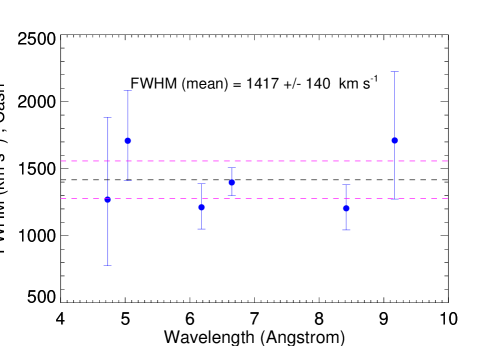
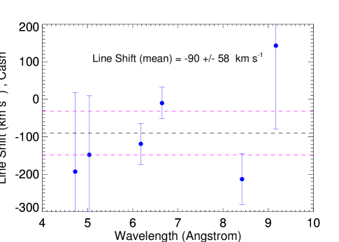
Figure 3: Spectral line parameters WR 48a.

Table 1: Line Parameters

Line	$\lambda_{lab}^{a}$	FWHMb	Line Shiftc	Fluxd	Ratio
	(Å)	( km s-1 )	( km s-1 )		(ATOMDB)
Fe XXV Kα	1.850	0e	398e	25.78${}^{+5.00}_{-4.58}$
(i/r)				0.44${}^{+0.37}_{-0.24}$	0.38
(f/r)				0.60${}^{+0.35}_{-0.24}$	0.30
S XVI Lα	4.727	1270${}^{+614}_{-494}$	-193${}^{+211}_{-186}$	11.86${}^{+3.82}_{-3.25}$
S XV Kα	5.039	1709${}^{+377}_{-298}$	-148${}^{+157}_{-152}$	58.56${}^{+5.53}_{-5.33}$
(i/r)				0.49${}^{+0.25}_{-0.22}$	0.23
(f/r)				0.64${}^{+0.17}_{-0.14}$	0.44
Si XIV Lα	6.180	1212${}^{+175}_{-163}$	-119${}^{+55}_{-55}$	25.93${}^{+2.36}_{-2.26}$
Si XIII Kα	6.648	1398${}^{+109}_{-99}$	-10${}^{+42}_{-42}$	72.02${}^{+3.58}_{-3.53}$
(i/r)				0.27${}^{+0.06}_{-0.05}$	0.20
(f/r)				0.75${}^{+0.07}_{-0.07}$	0.52
Mg XII Lα	8.419	1204${}^{+176}_{-161}$	-213${}^{+69}_{-68}$	15.45${}^{+1.87}_{-1.79}$
Mg XI Kα	9.169	1711${}^{+514}_{-437}$	143${}^{+220}_{-223}$	16.11${}^{+3.54}_{-3.36}$
(i/r)				0.05${}^{+0.23}_{-0.05}$	0.19
(f/r)				0.46${}^{+0.23}_{-0.17}$	0.59

Note. Results from the fits to the line profiles of emission lines in WR 48a with the associated $1\sigma$ errors. The first-order MEG and HEG spectra were fitted simultaneously for S XVI, S XV, Si XIV, Si XIII, and Mg XII lines, while only the HEG and MEG data were used for Fe XXV and MG XI, respectively. For the He-like triplets, the flux ratios of the intercombination to the resonance line (i/r) and of the forbidden to the resonance line (f/r) are given as well. The Cash statistic (Cash, 1979) was adopted in the fits.
^a The laboratory wavelength of the main component.
^b The line width (FWHM).
^c The shift of the spectral line centroid.
^d The observed total multiplet flux in units of $10^{-6}$ photons cm^-2 s^-1.
^e Because of the poor photon statistics, these line parameters are not constrained.

For each spectral line complex (H-like doublet or He-like triplet), we fitted the MEG and HEG spectra simultaneously sharing the same model parameters but the continuum level. In cases where the data quality was poor in either the MEG or HEG spectrum, we used only the better quality spectrum with more counts for fitting some He-like triplets: Fe XXV (HEG) and Mg XI (MEG)

It is quite common that the high resolution X-ray spectra have a very low number of counts (even zero counts) in the spectral bins. The photon statistics could be improved by re-binning the X-ray spectrum of a given object but this is at the expense of deteriorating the spectral resolution. To avoid this, we worked with the unbinned spectra (with no background subtracted) and made use of the Cash statistic (Cash, 1979) as implemented in xspec.

Figures 1, 2, 3 and Table 1 present the results from the fits to the line profiles in the grating spectra of WR 48a in 2019. We note that the parameters of the Fe XXV He-like triplet are not constrained with exception to the total observed line flux. On average, the X-ray emission lines are marginally blueshifted by $\sim 100$ km s^-1 . On the other hand, all the lines show a consistent line broadening of $\sim 1400$ km s^-1 . Forbidden lines in the He-like triplet do not seem to be suppressed, which is a sign that these spectral features form in hot plasmas with relatively low density and located far from strong sources of UV emission. The latter could be considered as a possible indication that these lines form in CSWs in wide massive binaries.

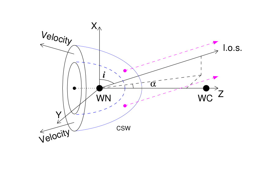
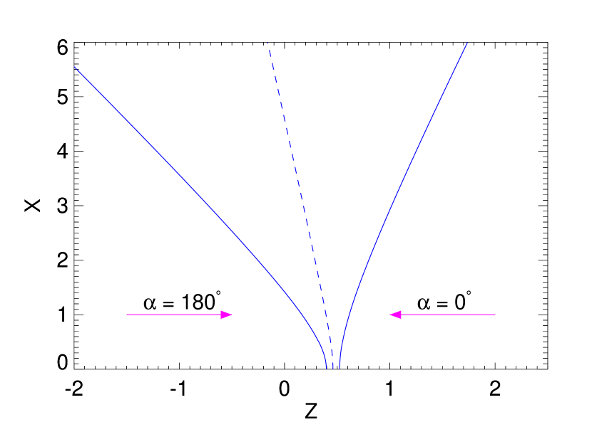
Figure 4: Left-hand panel: schematic presentation of the CSW region in the WC$+$WN binary WR 48a. The label CSW marks the wind interaction region, which is a 3D structure with its axis of symmetry Z. The axes X and Y complete the Cartesian coordinate system. The two angles $i$ (orbital inclination) and $\alpha$ (azimuthal angle) define the orientation in space of the line-of-sight (l.o.s.) towards observer. The label ‘Velocity’ denotes the general direction of the shocked plasma flow. The two dashed-line arrows illustrate that emission from a parcel of gas in the CSW region is subject to different wind absorption, depending on the orientation ($i$, $\alpha$) of the l.o.s. towards observer and the rotational angle around the axis of symmetry (Z). Right-hand panel: the CSW region derived from the 2D hydrodynamic simulations for the adopted values of the stellar-wind parameters in WR 48a which give a ram-pressure ratio of the stellar winds $\Lambda=(\dot{M}_{WC8}V_{WC8})/(\dot{M}_{WN8}V_{WC8}=1.44$. The x- and z-axis are in units of the binary separation. The WN and WC components are located at (x, z) coordinates (0,0) and (0,1), respectively. The solid lines mark the shock fronts and the dashed line marks the contact discontinuity.

4 CSW Spectral modelling

As mentioned above, the main goal of this study is to carry out a direct comparison of the X-ray spectrum of a massive binary with the CSW model. For a more complete comparison, we focus mostly on the spectra with high spectral resolution, namely, on modelling the first-order Chandra-HETG spectra of WR 48a, because they provide also pieces of kinematic information (through line profiles) of the X-ray emitting plasma. In the global spectral modelling discussed here, we make use of the $\chi^{2}$ statistic and adopt the default standard weighting as defined in xspec.

4.1 CSW model

The basic feature of the standard CSW model in massive binaries is that the two spherically symmetric stellar winds have collided at their terminal velocities. Therefore, the numerical hydrodynamic model is two-dimensional (2D). Fig. 4 shows a schematic diagram of CSWs in a wide WC $+$ WN massive binary (i.e., WR 48a, see Section 4.2).

Our xspec CSW model is based on the 2D numerical hydrodynamic model of adiabatic CSW by Lebedev & Myasnikov (1990) (see also Myasnikov & Zhekov 1993). It can take into account partial electron heating in strong shocks (see Zhekov & Skinner 2000), non-equilibrium ionization (NEI) effects (see Zhekov 2007), line broadening due to the bulk gas velocity of the emitting plasma (see Zhekov & Park 2010), the specific stellar wind absorption of both binary components along the line of sight to the observer (see Zhekov 2021), and the different chemical composition of both stellar winds.

For a detailed description of the CSW model and the fitting procedure with the CSW model in xspec, we refer to section 4.1 of Zhekov (2017) and section 4.1 of Zhekov (2021).

4.2 Adopted CSW model parameters for WR 48a 

As known (e.g., Myasnikov & Zhekov 1993 and references therein), the mass-loss rate and velocity of the stellar winds of the binary components and the binary separation determine the shape and structure of the CSW region. So, these are the basic input parameters for the hydrodynamic CSW model in massive binaries.

We note that Zhekov et al. (2014b) reported that WR 48a has an composite optical spectrum, which could be represented by a sum of two WR spectra (WC8 and WN8h). This analysis also showed that there are two considerably different gas flows in this object. Namely, the ‘cool’ lines (HeI and HI lines) had full width at half maximum of FWHM $\approx 1000$ km s^-1 , while those of high-excitation ionic species (e.g., CIV) have FWHM $\approx 2000$ km s^-1 (see fig.6 in Zhekov et al. 2014b). So, WR 48a is considered a WC8 + WN8 massive binary (e.g., see Zhekov et al. 2014b).

For the mass-loss rates of the binary components, we adopted the mean values for the single WC8 and WN8 stars with known Gaia distances (see table 1 in Sander et al. 2019 and table 1 in Hamann et al. 2019).

To estimate the binary separation in WR 48a, we adopted an orbital period of $\approx 32$ yr (Williams et al., 2012) and rescaled the semimajor axis of the prototype CSW binary WR 140 based on the Kepler’s third law and using the orbital parameters of WR 140 from Monnier et al. (2011): orbital period of 2896 days (7.93 yr) and semimajor axis of 14.73 au.

The adopted values of the stellar wind parameters and binary separation in WR 48a are: $\dot{M}_{WC8}=2.92\times 10^{-5}$ and $\dot{M}_{WN8}=4.05\times 10^{-5}$ ( M_⊙ yr^-1 ); V${}_{WC8}=2000$ and V${}_{WN8}=1000$ ( km s^-1 ); semimajor axis of 37.3 au.

Based on these parameters, we see that the CSW shocks in WR 48a are adiabatic (using equation 9 in Myasnikov & Zhekov 1993), the shock-heated plasma may have different electron and ion temperatures (T${}_{e}\neq$ T_i; using equation 1 in Zhekov & Skinner 2000), and the NEI effects are not important (using equation 1 in Zhekov 2007) that is the hot plasma in WR 48a is in collisional ionization equilibrium.

For consistency with the previous X-ray studies (Zhekov et al. 2011; Zhekov et al. 2014a), we adopted a distance of 4 kpc to WR 48a. We have to keep in mind that the Gaia DR2 (Data Release 2) distance to this object is not tightly constrained: $2.70^{+1.23}_{-0.67}$ kpc (Bailer-Jones et al., 2018); $2.27^{+0.92}_{-0.57}$ kpc (Rate & Crowther, 2020). Also, we might expect some appreciable changes in the distance estimates of WR 48a based on the parallax values of $0.3451\pm 0.1082$ mas (DR2; Gaia Collaboration et al. 2018) and $0.1933\pm 0.0462$ mas (Gaia EDR3, Early Data Release 3; Gaia Collaboration et al. 2021).

Table 2: WR 48a Spectral Fit Results (abundances)

	$\beta=1.0$	$\beta=0.2$
Mg	0.47 (0.03)	0.48 (0.03)
Si	0.49 (0.01)	0.48 (0.01)
S	1.06 (0.01)	1.04 (0.01)
Ar	0.28 (0.01)	0.27 (0.01)
Ca	0.16 (0.01)	0.16 (0.02)
Fe	0.44 (0.01)	0.51 (0.01)

Note. Abundance values derived from the CSW model simultaneous fits to the Chandra-MEG and HEG spectra. Labels $\beta=1.0$ and $\beta=0.2$ denote correspondingly the cases of full temperature equilibration and partial electron heating at the shock fronts. Given are the mean value for each element and its standard deviation for the total number of 26 model fits (13 values of $\alpha\in[0,180]$ degrees and 2 values of $i=60,90$ degrees, the derived abundances are with respect to their typical values adopted in this study, see Section 4.3).

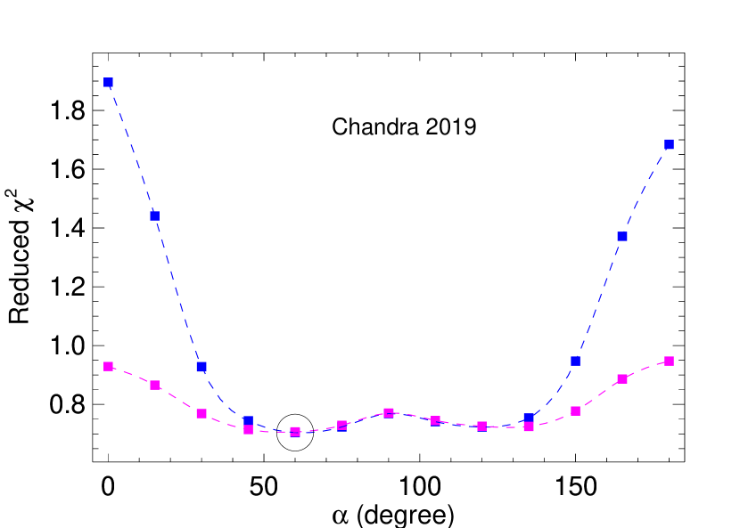
Figure 5: The reduced-$\chi^{2}$ values (degrees of freedom, dof = 251) vs. azimuthal angle ($\alpha$, see Fig. 4) for the case of equal electron and ion temperatures ($\beta=1$). The results for inclination angle of $i=90$ and $60$ degrees are shown in blue and magenta colour, respectively. The black circle marks the formal minimum value of the reduced $\chi^{2}$ at $\alpha=60$ degrees.

4.3 CSW model spectral results

Since the orbital parameters of WR 48a are not known and we have only an estimate of the binary separation (see Section 4.2), we explored a range of values for the azimuthal angle and orbital inclination (Fig. 4). We considered 13 equidistantly spaced values of $\alpha\in[0,180]$ degrees and two values of $i=60,90$ degrees. Due to the symmetry of the CSW region that resulted from interaction of two spherically-symmetric stellar winds, the CSW models with a given value of $\alpha$ and $360-\alpha$ give identical spectra. To see whether the partial electron heating at shock fronts could have any impact on the X-ray emission from WR 48a, we considered the cases of $\beta=1,0.2$ ($\beta=T_{e}/T$, $T_{e}$ is the electron temperature and $T$ is the mean plasma temperature).

We note that the X-ray spectrum of the CSW region is a sum of the X-ray emission from both shocked winds, which each may have different chemical composition. And, we recall that the CSW model is capable of taking into account the different chemical composition in both parts of the interaction region.

For the shocked WC and WN wind in the CSW region of WR 48a, we correspondingly adopted the abundance values typical for the WC and WN stars (by number) as from van der Hucht et al. (1986). Ar and Ca are not present in the van der Hucht et al. (1986) abundance sets, so, we adopted for each of them a fiducial value of $2\times 10^{-5}$.

For the WC shocked wind we adopted: H = 0.0, He = 1.0, C = 0.4, N = 0.0, O = 0.194, Ne = $1.86\times 10^{-2}$, Mg = $2.72\times 10^{-3}$, Si = $6.84\times 10^{-4}$, S = $1.52\times 10^{-4}$, Ar = $2\times 10^{-5}$, Ca = $2\times 10^{-5}$, Fe = $3.82\times 10^{-4}$.

And, for the WN shocked wind we adopted: H = 0.067, He = 1.0, C = $1.28\times 10^{-4}$, N = $.29\times 10^{-3}$, O = $2.92\times 10^{-4}$, Ne = $6.57\times 10^{-4}$, Mg = $2.19\times 10^{-4}$, Si = $2.16\times 10^{-4}$, S = $5.11\times 10^{-5}$, Ar = $2\times 10^{-5}$, Ca = $2\times 10^{-5}$, Fe = $1.28\times 10^{-4}$.

It is worth mentioning that both shocked winds have about comparable contribution to the total observed X-ray emission (flux) of WR 48a (see below). This is not surprising given the wind parameters of both stellar components that result in comparable ram pressure (see Section 4.2 and Fig. 4) and the fact that both winds are fast (e.g., were one of the winds slow, say $\sim 100$ km s^-1 , its shocked plasma would not have been a strong X-ray source). Also, for better quality of the fits, we allowed some abundances (Mg, Si, S, Ar, Ca, Fe) to vary. Since the X-ray emission from the shocked WC and WN winds cannot be disentangled, the abundance of a given element was varied by a single scaling parameter for both parts of the CSW region with respect to their reference abundances. These are the derived abundance values from the spectral fits.

Because chemical abundances are best constrained from dispersed X-ray spectra, we fitted simultaneously the MEG and HEG spectra of WR 48a. The fitting procedure consisted of the following steps, adopting our custom CSW model ($csw\_lines\_wind$) in xspec that takes into account line-broadening due to the bulk gas velocity of the hot plasma as well as stellar wind absorption along the line of sight.

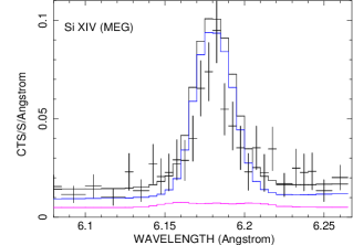
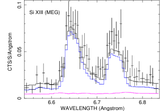
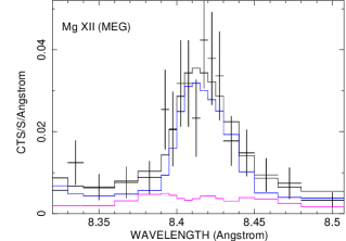
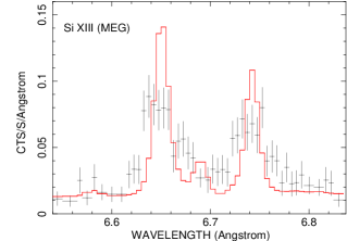
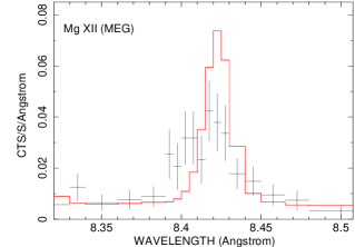
Figure 6: Top and middle panels. The MEG and HEG background-subtracted spectra of WR 48a and the best-fit CSW model ($\alpha=60$ degrees) near some strong emission lines. The WN and WC shocked stellar wind spectra are plotted in blue and magenta colour, respectively. Bottom panels. For comparison, shown are the MEG spectra overlaid with the CSW model for azimuthal angle $\alpha=0$ degrees and inclination angle $i=90$ degrees (the case of reduced $\chi^{2}=1.9$, see Fig. 5). The spectra were rebinned to have a minimum of 10 counts per bin.

(1) For each individual case ($\alpha,i,\beta$), we fitted the high-resolution spectra to estimate the abundances (the MEG and HEG spectra were rebinned to have a minimum of 20 counts per bin). To minimize the amount of CPU time, we used the xspec model gsmooth for the line broadening with a constant FWHM $=1400$ km s^-1 over the entire spectrum (see Section 3 and Fig. 3). So, the fitted xspec model is: $Spec=tbabs*gsmooth(csw\_lines\_wind)$ as the line-broadening was switched off in the $csw\_lines\_wind$ model. The tbabs model accounts for the interstellar (and circumstellar) absorption. The fit results showed that the derived abundance values for each chemical element have no big scatter: they have relatively small standard deviation around their corresponding mean value (see Table 2).

(2) For each value of $\beta$, we used the corresponding mean abundance values from Table 2 and we repeated all the spectral fits as described in step (1) with abundances kept fixed. We thus derived typical values for other CSW parameters: e.g., mass-loss scaling factor, X-rays absorption. It is worth noting that for both cases of $\beta$ the fractional mass-loss reduction was $\dot{M}_{s}\approx 0.27$ with respect to the nominal mass-loss values adopted in this study (see Section 4.2). On the other hand, the X-ray absorption is different between the cases of $\beta=1$ and $0.2$ and it also varies with the azimuthal angle. All this is well understood and we will further discuss it in Section 5.

(3) The best-fit models from step (2) were then used to check whether the CSW model provides the right kinematics of the X-ray emitting plasma in WR 48a. Namely, the fitted xspec model is: $Spec=tbabs*csw\_lines\_wind$ as the line broadening in the CSW model was switched on. Since the spectral line profiles provide information on the gas kinematics of the X-ray emitting plasma, we used the same spectral ranges for various emission lines as in the standard line fitting (see Section 3) to estimate correspondence between theory and observations, and these lines were considered (analysed) not one-by-one but simultaneously. Also, as a trade-off between spectral resolution and spectral quality we applied these models to the MEG and HEG spectra rebinned to have a minimum of 10 counts per bin.

Figure 5 presents the $\chi^{2}$ values for all the 26 cases under consideration and equal electron and ion temperatures ($\beta=1$). We note that we found no appreciable difference in the corresponding $\chi^{2}$ values between the cases of $\beta=1$ and $\beta=0.2$: the differences were less than 1%. Although the formal minimum of the reduced $\chi^{2}$ is at azimuthal angle of $\alpha=60$ degrees, we see that models in a broad range $\alpha\in[45,135]$ degrees could be considered acceptable for the quality of the 2019 Chandra-HETG spectra of WR 48a.

Examples of the direct confrontation of the observed line profiles in the X-ray spectrum of WR 48a and the CSW model are shown in Fig. 6. We see that although the CSW model does not provide a perfect match to the observed line profiles, the theoretical line profiles could be considered an acceptable representation of the observed line profiles of the strong line features in the X-ray spectrum of this CSW binary. An illustration of not acceptable theoretical profiles is shown in the bottom panels of Fig. 6 (the case of azimuthal angle $\alpha=0$ degrees and inclination angle $i=90$ degrees; the case of reduced $\chi^{2}=1.9$ in Fig. 5). These profiles are narrower than the observed ones and slightly redshifted with respect to them. This is a result from the considerably large opening angle of the CSW cone (see right-hand panel in Fig. 4). We have to keep in mind that the CSW cone has axial symmetry, but it is a 3D object. So, a parcel of hot gas, having the same plasma parameters, might be subject to different wind absorption depending on the rotational angle around the axis of symmetry of the CSW cone and the line-of-sight towards observer (e.g., left-hand panel in Fig. 4). This may result in symmetric or asymmetric line profiles and all these details are taken into account by the CSW model.

An interesting feature of the CSW model is that it can provide the contribution of each shocked stellar wind to the total X-ray emission from a CSW binary. For the case of WR 48a, we find that both shocked stellar winds have similar contribution to the total observed X-ray flux in the (0.5 - 10 keV) energy range: 54% (WN) and 46% (WC). But, the emission of the strong line features is dominated by the shocked WN stellar wind as illustrated in Fig. 6. This could be understood in the way that the plasma temperature in the WC part of the CSW region is considerably higher than that in the WN shocked plasma, thus, the WC shocked gas contributes mostly to the continuum emission. On the other hand, the WN shocked wind has the ‘right’ temperature to boost line emission. Of course, this is the case for the particular values of the wind velocities and chemical compositions adopted in this sudy.

Table 3: WR 48a Spectral Fit Results 2019 - 2008

	$\beta=1.0$			$\beta=0.2$
	2019	2012	2008	2019	2012	2008
$\chi^{2}$ (min - max)	274 - 288	56 - 57	809 - 994	265 - 283	54 - 55	645 - 778
dof	567	79	611	567	79	611
$\dot{M}_{s}$ (mass-loss reduction)	0.27 (0.01)	0.20 (0.01)	0.28 (0.01)	0.27 (0.01)	0.21 (0.01)	0.29 (0.01)
$F_{X}$ ($10^{-11}$ ergs cm-2 s-1)	0.95 (0.01)	0.36 (0.01)	1.01 (0.01)	0.91 (0.01)	0.34 (0.01)	0.98 (0.01)
$F_{0}$   ($10^{-11}$ ergs cm-2 s-1)	4.53 (0.11)	2.60 (0.04)	5.02 (0.16)	5.00 (0.12)	2.94 (0.04)	5.64 (0.17)
$\log L_{X}$ (ergs s-1)	34.94	34.70	34.98	34.98	34.75	35.03

Note. Results from the CSW model fits to the X-ray spectra of WR 48a:: Chandra 2019 (columns marked with 2019); Chandra 2012 (columns marked with 2012); XMM-Newton 2008 (columns marked with 2008). Labels $\beta=1.0$ and $\beta=0.2$ denote correspondingly the cases of full temperature equilibration and partial electron heating at the shock fronts. Tabulated quantities are the mass-loss scaling factor ($\dot{M}_{s}$), the observed X-ray flux ($F_{X}$), the unabsorbed (net) X-ray flux ($F_{0}$) and the logarithm of the X-ray luminosity ($\log L_{X}$) for an adopted distance of 4 kpc to WR 48a. The last three quantities are in the 0.5 - 10 keV energy range. Given are the mean values and their standard deviation for the total number of 26 model fits (13 values of $\alpha\in[0,180]$ degrees and 2 values of $i=60,90$ degrees, see Section 4.3).

5 Discussion

We carried out a direct modelling of the observed X-ray spectra with high spectral resolution (Chandra-HETG) of WR 48a in the framework of the standard colliding stellar wind picture in a massive WC+WN binary. Two of the most interesting CSW model results are the following.

First, a fractional mass-loss reduction of $\dot{M}_{s}\approx 0.27$ with respect to the nominal mass-loss values adopted in this study (see Section 4.2) is needed to match the observed X-ray flux. It was a result from the fact that the CSW model with the nominal mass-loss values predicted too high an emission measure (EM) for the X-ray plasma. It is worth recalling that in the case of spherically-symmetric stellar winds the emission measure in the CSW region is proportional to the square of the stellar wind mass loss ($\dot{M}$) and is reversely proportional to the binary separation ($a$): EM $\propto\dot{M}^{2}/a$ (e.g., see section 4.2 in Zhekov 2017). We note that this mass-loss reduction is related to the adopted distance of $d=4$ kpc to WR 48a (see Section 4.2). So, if the actual distance to WR 48a is smaller or larger than 4 kpc, then the amount of emission measure needed to match the observed X-ray flux will correspondingly decrease or increase ($\propto d^{2}$), so will the mass-loss reduction with respect to the value of $\dot{M}_{s}\approx 0.27$ ($\propto d$).

Second, the azimuthal angle of the observer was $\alpha=60$ degrees (see Fig. 4) or more likely it was in the range $\alpha\in[45,135]$ degrees as of 2019 November-December. On the other hand, the current knowledge of the stellar wind and binary parameters WR 48a did not allow us to obtain any constraints on the inclination angle of its binary orbit.

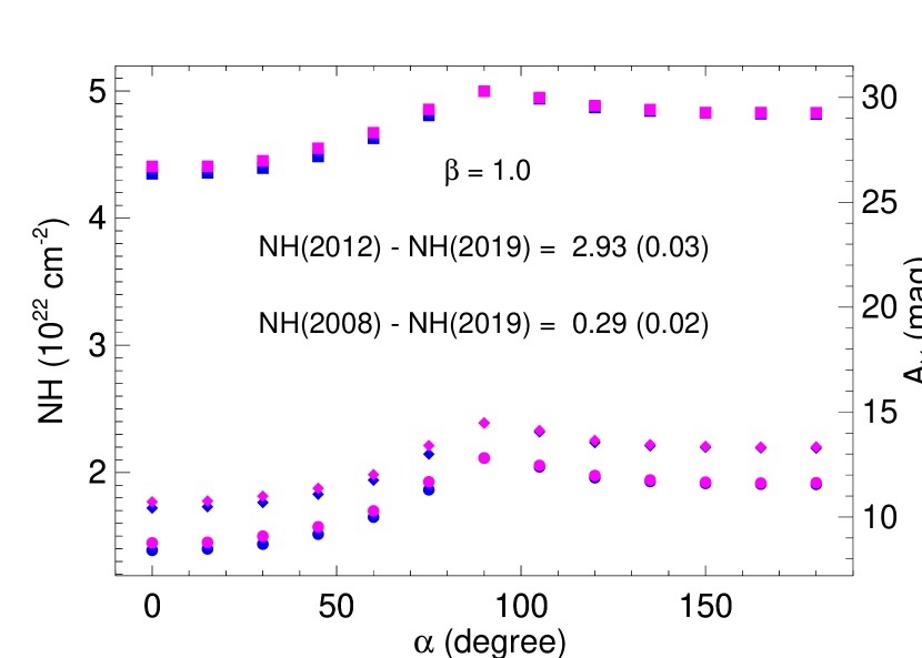
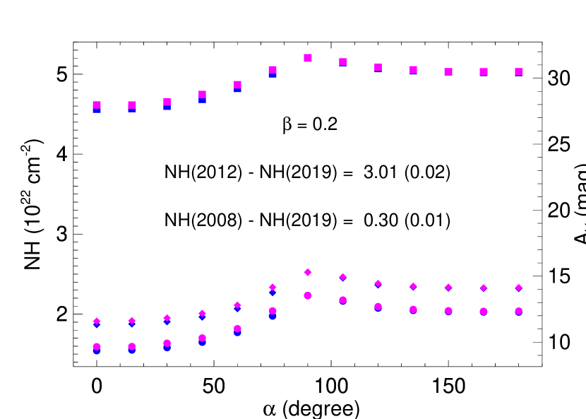
Figure 7: The X-ray absorption (NH) vs. azimuthal angle ($\alpha$, see Fig. 4). The results for inclination angle of $i=90$ and $60$ degrees are shown in blue and magenta colour, respectively. The bottom curves are for Chandra 2019, the curves in the middle are for XMM-Newton 2008 and the top curves are for Chandra 2012. The mean differences of the X-ray absorption and their standard deviations (in parentheses) are given as well.

However, in order to derive more constraints on the general CSW picture in WR 48a we think it could be a good idea to expand our current CSW-model analysis to other observations with good (or acceptable) quality. To do so, we made use of the previous X-ray observations of WR 48a as of 2008 January (XMM-Newton) and 2012 October (Chandra). Details on the standard X-ray analysis of these data sets are found in Zhekov et al. (2011) and Zhekov et al. (2014a). We may refer to these data sets as ‘XMM-Newton 2008’ and ‘Chandra 2012’ throughout the text.

Chandra 2012. This is a Chandra-HETG observation of WR 48a carried out on 2012 October 12 (Chandra Obs ID 13636). For the purpose of this analysis, we re-extracted the MEG and HEG spectra following the same data reduction recipe as for the Chandra 2019 data set (see Section 2). In the CSW model analysis, we made use of MEG and HEG spectra both re-binned to have a minimum of 10 and 20 counts per bin and we followed step (2) and (3) as described in Section 4.3 (i.e., adopting the abundance sets from Table 2). Due to the quality of the data (see Section 3; also fig. 2 in Zhekov et al. 2014a), only the MEG spectrum near the S XV, Si XIV and Si XIII lines was used in the step (3) of this analysis.

XMM-Newton 2008. This is an XMM-Newton observation of WR 48a carried out on 2008 January 9 (XMM-Newton Obs ID 0510980101). For the purpose of this analysis, we made use of the data from the pn detector of the European Photon Imaging Camera (EPIC). We used the XMM-Newton Science Analysis System (SAS, version 16.1.0) to filter the data for high X-ray background and to re-extract the source and background spectra and their corresponding response files. In the CSW model analysis, we used the pn spectrum re-binned to have a minimum of 100 counts per bin and we followed step (2) as described in Section 4.3, also adopting the abundance sets from Table 2.

Figure 8: The reduced-$\chi^{2}$ values (degrees of freedom, dof = 31) vs. azimuthal angle ($\alpha$, see Fig. 4) for the case of equal electron and ion temperatures ($\beta=1$). The results for inclination angle of $i=90$ and $60$ degrees are shown in blue and magenta colour, respectively. The black circle marks the formal minimum value of the reduced $\chi^{2}$ at $\alpha=105$ degrees.

Some results from the CSW-model fits to the Chandra 2012 and XMM-Newton 2008 spectra along with those for the Chandra 2019 spectra are given in Table 3, Figs. 7, 8 and 9. We immediately notice that the X-ray luminosity of WR 48a derived from the CSW-model analysis (Table 3) confirms its status of the most X-ray luminous Wolf-Rayet star in the Galaxy detected so far, after the black-hole candidate Cyg X-3 (Zhekov et al., 2011).

In the framework of the CSW picture, we also see that the observed characteristics of the X-ray emission region (i.e., the CSW zone) in WR 48a are quite similar in 2019 and 2008. On the other hand, it is confirmed what was already reported (Zhekov et al., 2014a) that the X-ray emission from WR 48a was appreciably lower in 2012 compared to its level in 2008. The same is valid for the amount of emission measure (EM $\propto\dot{M}_{s}^{2}$). It is also confirmed that the decrease of the emission measure in 2012 was accompanied with a considerable increase of the X-ray absorption.

We emphasize that the derived amount of X-ray absorption (Fig. 7) is in addition to that due to the stellar winds, that is it is of interstellar and circumstellar origin. The optical extinction toward WR 48a has been reported to be very high, A${}_{V}=9.2$ mag (Danks et al. 1983; see also fig. 8 in Zhekov et al. 2014b), and we note that a conversion N${}_{H}=1.65\,(1.6-1.7)\times 10^{21}$A_V cm^-2 (Vuong et al. 2003; Getman et al. 2005) is used in Fig. 7 (for the right-hand y-axis).

Figure 9: The background-subtracted spectra of WR 48a from different epochs overlaid with the best-fit CSW model. The Chandra and XMM-Newton spectra were re-binned to have a minimum of 20 and 100 counts per bin, respectively. The model spectra for $\beta=1$ and $0.2$ are plotted with red and green colour, respectively.

The apparent variation of the excess X-ray absorption with the azimuthal angle is a result from different chemical composition of the stellar winds. Namely, the more chemically evolved WC wind has a higher X-ray absorption than that of the WN wind, so, the additional X-ray absorption needed to match the shape of the X-ray spectrum is therefore smaller for azimuthal angles of $\alpha<90$ degrees. The opposite is valid for azimuthal angles of $\alpha>90$ degrees, when the WN component is predominantly ‘in front’. Naturally, the peak of the excess X-ray absorption is near $\alpha\approx 90$ degrees, when the stellar wind absorption is minimal (the observer’s line-of-sight is approximately ‘through’ the CSW region itself, i.e. along the x-axis in Fig. 4).

Figure 8 shows the results from confronting the CSW model profiles with the observed ones for Chandra 2012 for the case of equal electron and ion temperatures ($\beta=1$). As in the case of Chandra 2019 (see Section 4.3 and Fig. 5), we found no appreciable difference in the corresponding $\chi^{2}$ values between the cases of $\beta=1$ and $\beta=0.2$: the differences were less than 2%. The formal minimum of the reduced $\chi^{2}$ is at azimuthal angle of $\alpha=105$ degrees, but similarly to the case of the 2019 Chandra-HETG spectra of WR 48a, the models in a broad range (this time $\alpha\in[60,120]$ degrees) could be considered acceptable.

Finally, the case of partial electron heating at the strong shocks in the CSW region of WR 48a finds some support but only from the case of XMM-Newton 2008. We see that the quality of the CSW model fits for $\beta=0.2$ is better than that for $\beta=1$: the $\chi^{2}$ values of the former are by $\sim 25$% lower than those for the latter. Also as seen from Fig. 9, while there is practically no difference between the CSW model spectra with $\beta=1$ and $\beta=0.2$ for Chandra 2019 and Chandra 2012, that with equal electron and ion temperatures ($\beta=1$) predicts hard X-ray emission (wavelengths $<2$Å) higher than the observed one in XMM-Newton 2008. Since partial electron heating at shock fronts ($\beta<1$) results in ’on average’ lower electron temperature in the CSW region, the much larger effective area of the XMM-Newton-EPIC instruments helps detect some differences between X-ray spectra in the cases $\beta=1$ and $\beta=0.2$.

In general, we see that the CSW-model analysis of the X-ray spectra (with good quality: high spectral resolution, high photon statistics) of WR 48a provided some basic features of the CSW picture in this WC$+$WN massive binary. Namely, the observed X-ray emission from WR 48a is variable on long timescale (years) and the same is valid for its intrinsic X-ray emission. This requires variable mass-loss rates over its orbital period. And, the X-ray absorption is variable as well, as this absorption is in excess to that due to the stellar winds in the binary. It is worth noting that lower intrinsic X-ray emission is accompanied by higher X-ray absorption. Such a behaviour is quite similar to that of WR 140, which is the prototype of the CSW binaries showing periodic dust formation.

Namely, it is currently assumed that the dust formation in CSW binaries is set up near the periastron passage as illustrated by the case of WR 140 (Williams et al. 1990; also see Williams 1995, Williams 2008). Interestingly, the X-ray emission from this object decreases at about the same orbital phases correlating with an increase of the X-ray absorption (see Pollock et al. 2005; Pollock 2012).

An in-detail CSW-model analysis of the X-ray emission from WR 140 is presented in Zhekov (2021) showing that the mass-loss rates must decrease near periastron, and the following explanation was suggested. ‘The variable effective mass-loss rate could be understood qualitatively in CSW picture of clumpy stellar winds where clumps are efficiently dissolved in the CSW region near apastron but not at periastron. The increased X-ray absorption near periastron might be a sign of non-spherically symmetric stellar winds.’

In the framework of this qualitative CSW picture and following the time sequence of the WR 48a X-ray observations, we may assume that WR 48a was observed near periastron in 2012 (Chandra 2012), while it was observed quite a bit before and after periastron in 2008 (XMM-Newton 2008) and 2019 (Chandra 2019), respectively. The presumed periastron passage was likely at the end of 2011 (beginning of 2012) as maximum in the WR 48a light curve in the near infrared indicates (see fig. 3 in Williams et al. 2012). Interestingly, a minimum is present in the X-ray light curve of WR 48a at about the same period of time (see fig. 10 in Zhekov et al. 2014b; these short-exposure observations were carried out with the Swift observatory). And, we could add another detail in this qualitative picture.

Our analysis of the X-ray data on WR 48a with high spectral resolution (Chandra 2019; Chandra 2012) showed that the azimuthal angle of the line-ot-sight towards observer (Fig. 4) was in the broad range of $\alpha\in[45,135]$ and $\alpha\in[60,120]$ degrees in 2019 and in 2012, respectively.. Since such ranges are somehow ‘centred’ at the value of $\alpha=90$ degrees, it might be considered as an indication that this massive binary (WR 48a) is observed ‘pole-on’. We note that due to the axial symmetry of the CSW region all the spectra (line profiles) for azimuthal angle of $\alpha=90$ degrees and inclination angle $i\neq 0$ degrees are the same, and they are also identical to those with inclination angle $i=0$ degrees and arbitrary value of azimuthal angle. We have to keep in mind that even if WR 48a is observed ‘pole-on’, it will show variable X-ray emission provided its orbit has high eccentricity. By analogy with WR 140, the variable X-ray absorption (being the highest near periastron) could be a sign of non-spherically symmetric stellar winds.

We believe that more X-ray observations of massive binaries with high spectral resolution and good photon statistics as well as future development of CSW models with non-spherically symmetric winds may help us get a deeper insight of the CSW picture in these objects.

6 Conclusions

The basic results and conclusions from our analysis of the X-ray spectra of WR 48a with good quality (high spectral resolution, high photon statistics) are as follows.

(i) Analysis of the line profiles of strong emission features in the X-ray spectrum of WR 48a from recent Chandra-HETG observations (2019 November - December) showed that the spectral lines in this massive binary are broadened (typical FWHM of 1400 km s^-1 ) and marginally blueshifted by $\sim 100$ km s^-1 .

(ii) A direct modelling of these Chandra (MEG, HEG) spectra in the framework of the standard CSW picture provided a very good correspondence between the shape of the theoretical and observed spectra. Also, it showed that the theoretical line profiles are in most cases an acceptable representation of the observed ones. However, no tight constraints are derived on the azimuthal angle of the line-of-sight towards observer: it was in the range [45, 135] degrees at the time of observations.

(iii) To broaden this analysis, we applied the CSW model to the X-ray spectra of WR 48a from previous observations: Chandra-HETG (2012 October) and XMM-Newton (2008 January). The basic findings from the CSW modelling of all the three data sets are the following. The observed X-ray emission from WR 48a is variable on the long timescale (years) and the same is valid for its intrinsic X-ray emission. This requires variable mass-loss rates over the binary orbital period. The X-ray absorption is variable as well, as this absorption is in excess of that due to the stellar winds in the binary. Interestingly, lower intrinsic X-ray emission is accompanied by higher X-ray absorption.

(iv) The basic features described in the previous item are very similar to those found in the prototype CSW binary WR 140 based on the CSW modelling (see Zhekov 2021). By analogy with WR 140, we propose the same qualitative CSW picture for their explanation as given in Zhekov (2021). ‘The variable effective mass-loss rate could be understood in CSW picture of clumpy stellar winds where clumps are efficiently dissolved in the CSW region near apastron but not at periastron. The increased X-ray absorption near periastron might be a sign of non-spherically symmetric stellar winds.’

Data Availability

The X-ray data underlying this research are public and can be accessed as follows. The Chandra data sets can be downloaded from the Chandra X-ray observatory data archive https://cxc.harvard.edu/cda/ by typing in the target name (WR 48a) in the general search form https://cda.harvard.edu/chaser/. The XMM-Newton data sets can be downloaded from the XMM-Newton Science Archive by typing in the object name (WR 48a) in the general search form http://nxsa.esac.esa.int/nxsa-web/#search.

References

- Arnaud (1996) Arnaud K. A., 1996, in Jacoby G. H., Barnes J., eds, Astronomical Society of the Pacific Conference Series Vol. 101, Astronomical Data Analysis Software and Systems. p. 17
- Bailer-Jones et al. (2018) Bailer-Jones C. A. L., Rybizki J., Fouesneau M., Mantelet G., Andrae R., 2018, AJ, 156, 58
- Cash (1979) Cash W., 1979, ApJ, 228, 939
- Cherepashchuk (1976) Cherepashchuk A. M., 1976, Soviet Astronomy Letters, 2, 138
- Danks et al. (1983) Danks A. C., Dennefeld M., Wamsteker W., Shaver P. A., 1983, A&A, 118, 301
- Danks et al. (1984) Danks A. C., Wamsteker W., Shaver P. A., Retallack D. S., 1984, A&A, 132, 301
- Gaia Collaboration et al. (2018) Gaia Collaboration et al., 2018, A&A, 616, A1
- Gaia Collaboration et al. (2021) Gaia Collaboration et al., 2021, A&A, 649, A9
- Getman et al. (2005) Getman K. V., Feigelson E. D., Grosso N., McCaughrean M. J., Micela G., Broos P., Garmire G., Townsley L., 2005, ApJS, 160, 353
- Gosset et al. (2005) Gosset E., Nazé Y., Claeskens J. F., Rauw G., Vreux J. M., Sana H., 2005, A&A, 429, 685
- Hamann et al. (2019) Hamann W. R., et al., 2019, A&A, 625, A57
- Lebedev & Myasnikov (1990) Lebedev M. G., Myasnikov A. V., 1990, Fluid Dynamics, 25
- Monnier et al. (2011) Monnier J. D., et al., 2011, ApJ, 742, L1
- Myasnikov & Zhekov (1993) Myasnikov A. V., Zhekov S. A., 1993, MNRAS, 260, 221
- Oskinova et al. (2003) Oskinova L. M., Ignace R., Hamann W.-R., Pollock A. M. T., Brown J. C., 2003, A&A, 402, 755
- Pollock (1987) Pollock A. M. T., 1987, ApJ, 320, 283
- Pollock (2012) Pollock A. M. T., 2012, in Drissen L., Robert C., St-Louis N., Moffat A. F. J., eds, Astronomical Society of the Pacific Conference Series Vol. 465, Proceedings of a Scientific Meeting in Honor of Anthony F. J. Moffat, Astronomical Society of the Pacific, San Francisco. p. 308
- Pollock et al. (2005) Pollock A. M. T., Corcoran M. F., Stevens I. R., Williams P. M., 2005, ApJ, 629, 482
- Prilutskii & Usov (1976) Prilutskii O. F., Usov V. V., 1976, Soviet Ast., 20, 2
- Rate & Crowther (2020) Rate G., Crowther P. A., 2020, MNRAS, 493, 1512
- Rauw & Nazé (2016) Rauw G., Nazé Y., 2016, Advances in Space Research, 58, 761
- Sander et al. (2019) Sander A. A. C., Hamann W. R., Todt H., Hainich R., Shenar T., Ramachandran V., Oskinova L. M., 2019, A&A, 621, A92
- Skinner et al. (2006) Skinner S., Güdel M., Schmutz W., Zhekov S., 2006, Ap&SS, 304, 97
- Skinner et al. (2012) Skinner S. L., Zhekov S. A., Güdel M., Schmutz W., Sokal K. R., 2012, AJ, 143, 116
- Skinner et al. (2021) Skinner S. L., Schmutz W., Güdel M., Zhekov S. A., 2021, Research Notes of the American Astronomical Society, 5, 125
- Townsley et al. (2019) Townsley L. K., Broos P. S., Garmire G. P., Povich M. S., 2019, ApJS, 244, 28
- van der Hucht et al. (1986) van der Hucht K. A., Cassinelli J. P., Williams P. M., 1986, A&A, 168, 111
- Vuong et al. (2003) Vuong M. H., Montmerle T., Grosso N., Feigelson E. D., Verstraete L., Ozawa H., 2003, A&A, 408, 581
- Williams (1995) Williams P. M., 1995, in van der Hucht K. A., Williams P. M., eds, Proc. IAU Symposium Vol. 163, Wolf-Rayet Stars: Binaries; Colliding Winds; Evolution, Kluwer, Dordrecht. p. 335
- Williams (2008) Williams P. M., 2008, in Benaglia P., Bosch G. L., C.A. C., eds, Revista Mexicana de Astronomia y Astrofisica Conference Series Vol. 33, Proc. Conf. Massive Stars: Fundamental Parameters and Circumstellar Interactions. p. 71
- Williams et al. (1990) Williams P. M., van der Hucht K. A., Pollock A. M. T., Florkowski D. R., van der Woerd H., Wamsteker W. M., 1990, MNRAS, 243, 662
- Williams et al. (2012) Williams P. M., van der Hucht K. A., van Wyk F., Marang F., Whitelock P. A., Bouchet P., Setia Gunawan D. Y. A., 2012, MNRAS, 420, 2526
- Zhekov (2007) Zhekov S. A., 2007, MNRAS, 382, 886
- Zhekov (2017) Zhekov S. A., 2017, MNRAS, 472, 4374
- Zhekov (2021) Zhekov S. A., 2021, MNRAS, 500, 4837
- Zhekov & Park (2010) Zhekov S. A., Park S., 2010, ApJ, 721, 518
- Zhekov & Skinner (2000) Zhekov S. A., Skinner S. L., 2000, ApJ, 538, 808
- Zhekov et al. (2011) Zhekov S. A., Gagné M., Skinner S. L., 2011, ApJ, 727, L17
- Zhekov et al. (2014a) Zhekov S. A., Gagné M., Skinner S. L., 2014a, ApJ, 785, 8
- Zhekov et al. (2014b) Zhekov S. A., Tomov T., Gawronski M. P., Georgiev L. N., Borissova J., Kurtev R., Gagné M., Hajduk M., 2014b, MNRAS, 445, 1663