Energy norm analysis of exactly symmetric mixed finite elements for linear elasticity

Abstract.

We consider mixed finite element methods for linear elasticity for which the symmetry of the stress tensor is exactly satisfied. We derive a new quasi-optimal a priori error estimate uniformly valid with respect to the compressibility. For the a posteriori error analysis we consider the Prager-Synge hypercircle principle and introduce a new estimate uniformly valid in the incompressible limit. All estimates are validated by numerical examples.

1. Introduction

The purpose of this paper is to provide an analysis of mixed finite element methods for linear elasticity. By mixed methods we mean methods based on the principle of minimum of the complementary energy, i.e. methods in which the strain energy is expressed with the stress tensor and the equation of static equilibrium acts as a constraint. The Lagrange multiplier connected to this constraint is the displacement vector. By an integration by parts, this formulation is dual to the standard formulation of minimizing the total energy where Dirichlet boundary condition for the displacement now become natural and traction conditions are enforced. A crucial property of this class of methods is that each element is point wise in mechanical equilibrium and along each element edge or face the traction vector is continuous. These conditions are naturally very appealing, and that was the original motivation to develop the methods in the engineering community [17, 38]. The formulation can be traced by various energy methods classically used in elastostatics, cf. [11]. The first mathematical treatment of this principle was done by Friedrichs [18] (cf. also [14, Chapter IV.9]).

Mathematically, the methods (and the corresponding simpler methods for scalar second order problems) have been analyzed thoroughly, and the literature is voluminous as can be seen from the monograph by Boffi, Brezzi and Fortin [12]. The analysis framework usually used is the one laid down in the pioneering work by Raviart and Thomas [30]. More recently, tools of differential exterior calculus has been used to gain insight into the methods [5], which has lead to numerous new methods. These analyses uses the $H(\mathrm{div}\,\!)$ and $L^{2}$ norms for the stress and the displacement, respectively. From a mechanical point of view this can be seen as unnatural since the norms do not have any physical meaning and hence blur the origin of the methods, the minimization of the strain energy. In our analysis we derive the estimates in energy, or closely related, norms. This approach was initiated in a classical paper by Babuška, Osborn and Pitkäranta [6]. For the elasticity problem their technique of mesh dependent norms was first used by Pitkäranta and Stenberg [28]. The norms used are basically the energy norm for the stresses and a broken energy norm for the displacement. The broken $H^{1}$ norm dates back, at least, to the early works on interior penalty methods, cf. Arnold [1], Douglas and Dupont [16] and Baker [8]. During the last decades the interior penalty methods have received considerable attention, now under the name of discontinuous Galerkin methods, cf. [15].

The equilibrium property enables the error in the stress to be decoupled from that of the displacement (which is of lower order). However, it also leads to a superconvergence estimate for the difference between the finite element solution and the $L^{2}$ projection of the displacement. Brezzi and Arnold where the first to observe that this can be used in a local postprocessing yielding a more accurate approximation [3]. In Lovadina and Stenberg [26] it was shown that this leads to a simple a posteriori error estimate.

In this paper we first collect the techniques and results mentioned above. In addition, we improve and extend the analysis. For the a priori analysis we use Gudi’s trick for DG methods [20] in order to improve the estimate removing the flaw that the exact stress should be in $H^{s}$, with $s>1/2$. In addition, we use a second postprocessing, the so-called Oswald interpolation [15], to obtain a kinematically admissible displacement, i.e. continuous and satisfying the Dirichlet boundary conditions. With this we utilize the classical hypercircle principle of Prager and Synge [29, 27], which states with a kinematically admissible displacement and a statically admissible stress approximation, i.e. one with exact satisfaction of the equilibrium and traction boundary conditions, it is possible to get an a posteriori estimate in the form of an equality. This idea we use to derive an a posteriori estimate that includes oscillation terms in the case when the equilibrium and the traction boundary are satisfied only approximately.

One attractive feature of mixed methods is that they are robust also in the incompressible limit. For the a priori estimate this is a consequence of the ellipticity in the kernel in Brezzi’s theory of saddle point problems which is valid. The Prager-Synge hypercircle estimate, however, breaks down near incompressibility. For this case we introduce a novel a posteriori estimate.

The plan of the paper is the following: in the next two sections we first recall the elasticity problem and then discuss its mixed approximation. We concretize it by the Watwood-Hartz (or Johnson-Mercier) [38, 23] method, and the families of Arnold-Douglas-Gupta [4] and Arnold-Awanou-Winther [2]. Then we derive the a priori estimates for both the stress and the post processed displacement in Section 4 an Section 5, respectively. In Section 6 we prove both the Prager-Synge and our new a posteriori estimate. In the final section numerical results are given.

In a subsequent paper [25], we will consider mixed methods with the symmetry of the stress tensor enforced in a weak sense.

We use the established notation for Sobolev spaces and finite element methods. We write $A\lesssim B$ when there exist a positive constant $C$, that is independent of the mesh parameter and in particular of the two Lamé parameters $\mu,\lambda$ (see below) such that $A\leq CB$. Analogously we define $A\gtrsim B$. This means that the dependency of the two Lamé parameters are made explicit in the norms used.

2. The Equations of elasticity

Let $\Omega\subset{}^{d}$ be a polygonal or polyhedral domain. The physical unknowns are the displacement vector $u=(u_{1},\dots,u_{d})$ and the symmetric stress tensor $\sigma=\{\sigma_{ij}\}$, $\sigma_{ij}=\sigma_{ji}$, $i,j=1,\dots,d$. The stress tensor is related to the strain tensor

(2.1) $$\varepsilon(u),\quad\varepsilon(u)_{ij}=\frac{1}{2}\Big{(}\frac{\partial u_{i}}{\partial x_{j}}+\frac{\partial u_{j}}{\partial x_{i}}\Big{)},$$

by a linear constitutive law. In order to be explicit, we consider the plain strain ($d=2$) or 3D ($d=3$) problem for an isotropic material. We define the compliance matrix

(2.2) $$\mathcal{C}\tau=\frac{1}{2\mu}\Big{(}\tau-\frac{\lambda}{2\mu+d\lambda}{\rm tr}(\tau)I\Big{)},$$

with the Lamé parameters $\mu\mbox{ and }\lambda$. Then it holds

(2.3) $$\mathcal{C}\sigma+\varepsilon(u)=0.$$

The inverse of the compliance matrix, the elasticity matrix, we denote by ${\mathcal{A}}$, i.e.

(2.4) $${\mathcal{A}}\tau=\mathcal{C}^{-1}\tau=2\mu\tau+\lambda{\rm tr}(\tau)I.$$

In the limit $\lambda\to\infty$ the material becomes incompressible, i.e.

(2.5) $$\mathrm{div}\,u=0.$$

The loading consists of a body load $f$ and a traction $g$ on the boundary part $\Gamma_{N}$. On the complementary part $\Gamma_{D}$ homogeneous Dirichlet conditions for the displacement are given. The equations of elasticity in mixed form are then

(2.6) $$\mathcal{C}\sigma-\varepsilon(u) = 0\ \mbox{ in }\Omega,$$

(2.7) $$\mathrm{div}\,\sigma+f = 0\ \mbox{ in }\Omega,$$

(2.8) $$u = 0\ \mbox{ on }\Gamma_{D},$$

(2.9) $$\sigma n = g\ \mbox{ on }\Gamma_{N}.$$

For this system we use two variational formulations. The first is: find $\sigma\in[L^{2}(\Omega)]^{d\times d}_{{\rm sym}}$ and $u\in[H_{D}^{1}(\Omega)]^{d}=\{\,v\in[H^{1}(\Omega)]^{d}\,|\,v|_{\Gamma_{D}}=0\,\}$ such that

(2.10) $${\mathcal{B}}(\sigma,u;\tau,v)=(f,v)+\langle g,v\rangle_{\Gamma_{N}}\quad\forall(\tau,v)\in[L^{2}(\Omega)]^{d\times d}_{{\rm sym}}\times[H_{D}^{1}(\Omega)]^{d},$$

with the bilinear form

(2.11) $${\mathcal{B}}(\sigma,u;\tau,v)=(\mathcal{C}\sigma,\tau)-(\varepsilon(u),\tau)-(\varepsilon(v),\sigma).$$

Physically, the natural norms for analyzing this problem are

(2.12) $$\|\tau\|_{\mathcal{C}}^{2}=(\mathcal{C}\sigma,\sigma)\ \mbox{ and }\ \|\varepsilon(u)\|_{\mathcal{A}}^{2}=({\mathcal{A}}\varepsilon(u),\varepsilon(u)),$$

which are twice the strain energy expressed by the stress and displacement, respectively. The Babuška–Brezzi condition is then simply the identity

(2.13) $$\sup_{\tau\in[L^{2}(\Omega)]^{d\times d}_{{\rm sym}}}\frac{\big{(}\tau,\varepsilon(v)\big{)}}{\|\tau\|_{\mathcal{C}}}=\|\varepsilon(v)\|_{\mathcal{A}}\quad\forall v\in[H_{D}^{1}(\Omega)]^{d}.$$

This gives the following stability estimate (with a known constant, cf. [22])

(2.14) $$\sup_{\eta\in[L^{2}(\Omega)]^{d\times d}_{{\rm sym}}\atop z\in[H_{D}^{1}(\Omega)]^{d}} \frac{{\mathcal{B}}(\tau,v;\eta,z)}{\big{(}\|\eta\|_{\mathcal{C}}^{2}+\|\varepsilon(z)\|_{\mathcal{A}}^{2}\big{)}^{1/2}}\geq\Big{(}\frac{\sqrt{5}-1}{2}\Big{)}\Big{(}\|\tau\|_{\mathcal{C}}^{2}+\|\varepsilon(v)\|_{\mathcal{A}}^{2}\Big{)}^{1/2}$$

$$\qquad\qquad\forall(\tau,v)\in[L^{2}(\Omega)]^{d\times d}_{{\rm sym}}\times[H_{D}^{1}(\Omega)]^{d}.$$

In the incompressible limit $\|\cdot\|_{\mathcal{C}}$ does not, however, define a norm, and the full stability is a consequence of the ellipticity in the kernel. Instead of using the abstract theory of Brezzi [12], we give an explicit proof of stability. More precisely, for $\tau$ we let $\tau^{D}$ be the deviatoric part of $\tau$, defined by the condition ${\rm tr}(\tau^{D})=0.$ Hence it holds

(2.15) $$\tau=\tau^{D}+\frac{1}{d}{\rm tr}(\tau)I.$$

By a direct computation we get.

Lemma 1.

It holds that

(2.16) $$(\mathcal{C}\tau,\tau)=\frac{1}{2\mu}\|\tau^{D}\|_{0}^{2}+\frac{1}{2\mu+d\lambda}\|{\rm tr}(\tau)\|_{0}^{2}.$$

From this it is seen that when $\lambda\to\infty$, $\|\cdot\|_{\mathcal{C}}$ does not give control over the pressure part (the trace) of the stress tensor.

To derive estimates valid independently of $\lambda$ we use the norms

(2.17) $$\mu^{-1/2}\|\tau\|_{0}\ \mbox{ for }\tau\in[L^{2}(\Omega)]^{d\times d}_{{\rm sym}},\ \mbox{ and}\ \mu^{1/2}\|\varepsilon(v)\|_{0}\ \mbox{ for }v\in[H_{D}^{1}(\Omega)]^{d}.$$

For the stability estimate the Babuška–Brezzi condition for the Stokes problem [19]

(2.18) $$\sup_{v\in[H_{D}^{1}(\Omega)]^{d}}\frac{(\mathrm{div}\,v,q)}{\|\varepsilon(v)\|_{0}}\geq\beta\|q\|_{0}\quad\forall q\in L^{2}(\Omega),s$$

is needed. Using this we prove the following stability estimate.

Theorem 1.

It holds that

(2.19) $$\sup_{\eta\in[L^{2}(\Omega)]^{d\times d}_{{\rm sym}}\atop z\in[H_{D}^{1}(\Omega)]^{d}}\ \frac{{\mathcal{B}}(\tau,v;\eta,z)}{\big{(}\mu^{-1}\|\eta\|_{0}^{2}+\mu\|\varepsilon(z)\|_{0}^{2}\big{)}^{1/2}} \gtrsim\big{(}\mu^{-1}\|\tau\|_{0}^{2}+\mu\|\varepsilon(v)\|_{0}^{2}\big{)}^{1/2}$$

$$\forall(\tau,v)\in[L^{2}(\Omega)]^{d\times d}_{{\rm sym}}\times[H_{D}^{1}(\Omega)]^{d}.$$

Proof.

Let $(\tau,v)$ be given. By (2.18) there exists $z\in[H_{D}^{1}(\Omega)]^{d}$ such that

(2.20) $$(\mathrm{div}\,z,{\rm tr}(\tau))\geq\beta\|{\rm tr}(\tau)\|_{0}^{2}\quad\mbox{and }\|\varepsilon(z)\|_{0}=\|{\rm tr}(\tau)\|_{0}.$$

Let $\delta>0$ and $\gamma>0$. By the bilinearity we have

(2.21) $${\mathcal{B}}( \tau,v;\tau-\gamma\varepsilon(v),-v-\delta z)$$

$$= {\mathcal{B}}(\tau,v;\tau,-v)-\gamma{\mathcal{B}}(\tau,v;\varepsilon(v),0)-\delta{\mathcal{B}}(\tau,v;0,z).$$

For the first term we have

(2.22) $${\mathcal{B}}(\tau,v;\tau,-v)=(\mathcal{C}\tau,\tau)=\frac{1}{2\mu}\|\tau^{D}\|_{0}^{2}+\frac{1}{2\mu+d\lambda}\|{\rm tr}(\tau)\|_{0}^{2}.$$

From (2.2) we have

(2.23) $$\|\mathcal{C}\tau\|_{0}\leq\frac{1}{2\mu}\Big{(}\|\tau\|_{0}+\frac{1}{d}\|{\rm tr}(\tau)I\|_{0}\Big{)}\leq\frac{1}{\mu}\|\tau\|_{0}.$$

Using the Schwarz and Young inequalities then gives

(2.24) $$-\gamma{\mathcal{B}}(\tau,v;\varepsilon(v),0) =-\gamma(\mathcal{C}\tau,\varepsilon(v))+\gamma\|\varepsilon(v)\|_{0}^{2}\geq-\frac{\gamma}{2}\|\mathcal{C}\tau\|_{0}^{2}+\frac{\gamma}{2}\|\varepsilon(v)\|_{0}^{2}$$

$$\geq-\frac{\gamma}{2\mu^{2}}\|\tau\|_{0}^{2}+\frac{\gamma}{2}\|\varepsilon(v)\|_{0}^{2}.$$

By (2.20) we have

(2.25) $$-\delta {\mathcal{B}}(\tau,v;0,z)=\delta(\tau,\varepsilon(z))=\frac{\delta}{d}({\rm tr}(\tau),\mathrm{div}\,z)+\delta(\tau^{D},\varepsilon(z))$$

$$\geq\frac{\delta\beta}{d}\|{\rm tr}(\tau)\|_{0}^{2}+\delta(\tau^{D},\varepsilon(z))\geq\frac{\delta\beta}{d}\|{\rm tr}(\tau)\|_{0}^{2}-\delta\|\tau^{D}\|_{0}\|\varepsilon(z)\|_{0}$$

$$=\frac{\delta\beta}{d}\|{\rm tr}(\tau)\|_{0}^{2}-\delta\|\tau^{D}\|_{0}\|{\rm tr}(\tau)\|_{0}$$

$$\geq\frac{\delta\beta}{2d}\|{\rm tr}(\tau)\|_{0}^{2}-\frac{\delta d}{2\beta}\|\tau^{D}\|_{0}^{2}.$$

Collecting the above estimates, we get

(2.26) $${\mathcal{B}}( \tau,v;\tau-\gamma\varepsilon(v),-v-\delta z)$$

$$\geq \Big{(}\frac{1}{2\mu}-\frac{\delta d}{2\beta}\Big{)}\|\tau^{D}\|_{0}^{2}+\Big{(}\frac{1}{2\mu+d\lambda}+\frac{\delta\beta}{2d}\Big{)}\|{\rm tr}(\tau)\|_{0}^{2}$$

$$-\frac{\gamma}{2\mu^{2}}\|\tau\|_{0}^{2}+\frac{\gamma}{2}\|\varepsilon(v)\|_{0}^{2}.$$

Now we choose $\delta=\frac{\beta}{2\mu d}$, which gives

(2.27) $${\mathcal{B}}( \tau,v;\tau-\gamma\varepsilon(v),-v-\delta z)$$

$$\geq \frac{1}{4\mu}\|\tau^{D}\|_{0}^{2}+\Big{(}\frac{1}{2\mu+d\lambda}+\frac{\beta^{2}}{4d^{2}\mu}\Big{)}\|{\rm tr}(\tau)\|_{0}^{2}-\frac{\gamma}{2\mu^{2}}\|\tau\|_{0}^{2}+\frac{\gamma}{2}\|\varepsilon(v)\|_{0}^{2}.$$

Let $C>0$ such that

(2.28) $$\frac{1}{4\mu}\|\tau^{D}\|_{0}^{2}+\Big{(}\frac{1}{2\mu+d\lambda}+\frac{\beta^{2}}{4d^{2}\mu}\Big{)}\|{\rm tr}(\tau)\|_{0}^{2}\geq\frac{C}{\mu}\|\tau\|_{0}^{2},$$

and choose $\gamma=C\mu$. This gives

(2.29) $$B(\tau,v;\tau-\gamma\varepsilon(v),-v-\delta z)\geq\frac{C}{2}\Big{(}\mu^{-1}\|\tau\|_{0}^{2}+\mu\|\varepsilon(v)\|_{0}^{2}\Big{)}.$$

It also holds

(2.30) $$\mu^{-1}\|\tau-\gamma\varepsilon(v)\|_{0}^{2}+\mu\|\varepsilon(v+\delta z)\|_{0}^{2}\lesssim\mu^{-1}\|\tau\|_{0}^{2}+\mu\|\varepsilon(v)\|_{0}^{2},$$

which proves the asserted estimate. $\Box$

The second variational form is the basis for the mixed finite element method. By dualisation the stress is in

(2.31) $$H(\mathrm{div}\!:\!\Omega)=\{\,\tau\in[L^{2}(\Omega)]^{d\times d}_{{\rm sym}}\,|\,\mathrm{div}\,\tau\in[L^{2}(\Omega)]^{d}\,\},$$

the displacement in $[L^{2}(\Omega)]^{d}$, and the bilinear form used is

(2.32) $${\mathcal{M}}(\sigma,u;\tau,v)=(\mathcal{C}\sigma,\tau)+(u,\mathrm{div}\,\tau)+(v,\mathrm{div}\,\sigma),$$

and the formulation is: find $\sigma\in H_{g}(\mathrm{div}\,\!\!:\!\Omega)$ and $u\in[L^{2}(\Omega)]^{d}$, such that

(2.33) $${\mathcal{M}}(\sigma,u;\tau,v)+(f,v)=0\quad\forall(\tau,v)\in H_{0}(\mathrm{div}\,\!\!:\!\Omega)\times[L^{2}(\Omega)]^{d},$$

with

(2.34) $$H_{g}(\mathrm{div}\,\!\!:\!\Omega)=\{\,\tau\in H({\rm div}\!:\!\Omega)\,|\ \tau n|_{\Gamma_{N}}=g\,\},$$

and

(2.35) $$H_{0}(\mathrm{div}\,\!\!:\!\Omega)=\{\,\tau\in H({\rm div}\!:\!\Omega)\,|\ \tau n|_{\Gamma_{N}}=0\,\}.$$

3. Exactly symmetric mixed finite element methods

The mixed finite element method is based on the variational formulation (2.33) using piecewise polynomial subspaces $V_{h}\subset[L^{2}(\Omega)]^{d}$ and $S_{h}\subset H(\mathrm{div}\!:\!\Omega)$. We give a unified presentation that covers the following methods:

• The linear triangular method of Johnson–Mercier (JM) [23, 38].

• The triangular family of Arnold–Douglas–Gupta [4].

• The triangular family of Guzman–Neilan  [21].

• The tetrahedral family of Arnold–Awanou–Winther [2].

The triangular or tetrahedral mesh is denoted by ${\mathcal{C}}_{h}$. The families are indexed by the polynomial degree $k\geq 2$ and the displacement space is simply

(3.1) $$V_{h}=\{\,v\in[L^{2}(\Omega)]^{d}\,|\ v|_{K}\in[P_{k-1}(K)]^{d}\ \forall K\in{\mathcal{C}}_{h}\,\}.$$

For the JM method the space in (3.1) appears with $k=2$, i.e. discontinuous piecewise linear polynomials are used.

The spaces for the stress are defined by

(3.2) $$S_{h}=\{\,\tau\in H(\mathrm{div}\!:\!\Omega)\,|\,\tau|_{K}\in S(K)\,\forall K\in{\mathcal{C}}_{h}\,\}.$$

The local spaces $S(K)$ are rather involved and here we will not give the explicitly definitions. The essential properties are, however, the right approximation order which is ensured by the inclusion

(3.3) $$[P_{k}(K)]^{n\times n}_{\mathrm{sym}}\subset S(K),$$

and the degrees of freedom needed for the stability; the local degrees of freedom of $\tau\in S(K)$ contain the moments

(3.4) $$\int_{K}\tau:\varepsilon(v)\quad\forall v\in[P_{k-1}(K)]^{d},$$

and

(3.5) $$\int_{E}\tau n\cdot v\quad\forall v\in[P_{k}(E)]^{d},$$

for each edge or face $E$ of $K$. For the JM method (3.3), (3.4) and (3.5) are valid with $k=1$.

For all spaces, except JM, we have

(3.6) $$\mathrm{div}\,\tau\in V_{h}\quad\forall\tau\in S_{h},$$

and hence for these it holds

(3.7) $$(\mathrm{div}\,\tau,v-P_{h}v)=0\quad\forall\tau\in S_{h},$$

where $P_{h}:[L^{2}(\Omega)]^{d}\to V_{h}$ denotes the $L^{2}$-projection. For JM (3.6) does not hold. However, it is easily seen that if $\tau\in S(K)$ satisfies

(3.8) $$(\mathrm{div}\,\tau,v)_{K}=0\quad\mbox{for }v\in[P_{1}(K)]^{2}$$

then $\mathrm{div}\,\tau=0$ on $K$. By this there exist a projection with the property (3.7), cf. [23, Lemma 2] and [28, Lemma 4.3].

For an edge/face $E\subset\Gamma_{N}$ we let $Q_{E}:[L^{2}(E)]^{d}\to[P_{k}(E)]^{d}$ denote the $L^{2}$ projection and define the operator $Q_{h}$ by $Q_{h}|_{E}=Q_{E}$.

The trial and test finite element spaces are then defined as

(3.9) $$S_{h}^{g} =\{\,\tau\in S_{h}\,|\,\tau n=Q_{h}g\mbox{ on }\Gamma_{N}\,\},$$

$$\ S_{h}^{0} =\{\,\tau\in S_{h}\,|\,\tau n=0\mbox{ on }\Gamma_{N}\,\}.$$

The mixed finite element method is: find $(\sigma_{h},u_{h})\in S_{h}^{g}\times V_{h}$ such that

(3.10) $${\mathcal{M}}(\sigma_{h},u_{h};\tau,v)+(f,v)=0\quad\forall(\tau,v)\in S_{h}^{0}\times V_{h}.$$

4. Stability and a priori error analysis

In this section we will derive a priori error estimates. For the displacement we use the following broken energy norm, first introduced in [28, 33]. Here $\Gamma_{h}$ denotes the edges/faces in the interior of $\Omega$.

(4.1) $$\|v\|_{h}^{2}=\sum_{K\in{\mathcal{C}}_{h}}\|\varepsilon(v)\|_{0,K}^{2}+\sum_{E\in\Gamma_{h}}h_{E}^{-1}\|[\![v]\!]\|_{0,E}^{2}+\sum_{E\subset\Gamma_{D}}h_{E}^{-1}\|v\|_{0,E}^{2}\quad v\in V_{h}.$$

The stability of the method is proven by the following two conditions.

Lemma 2.

It holds that

(4.2) $$\sup_{\tau\in S_{h}^{0}}\frac{\big{(}\mathrm{div}\,\tau,v\big{)}}{\|\tau\|_{0}}\gtrsim\|v\|_{h}\quad\forall v\in V_{h}.$$

Proof.

Let $v\in V_{h}$ be given. We choose $\tau\in S_{h}^{0}$ such that all degrees of freedom vanish, except (3.4) and (3.5) which are chosen such that

(4.3) $$\int_{K}\tau:\varepsilon(v)=\int_{K}|\varepsilon(v)|^{2}\quad\forall K\in{\mathcal{C}}_{h},$$

(4.4) $$\int_{E}\tau n\cdot v=h_{E}^{-1}\int_{E}|[\![v]\!]|^{2}\quad\forall E\in\Gamma_{h},$$

and

(4.5) $$\int_{E}\tau n\cdot v=h_{E}^{-1}\int_{E}|v|^{2}\quad\forall E\subset\Gamma_{D}.$$

Hence

(4.6) $$(\mathrm{div}\,\tau,v)=\|v\|_{h}^{2}.$$

By scaling it holds

(4.7) $$\|\tau\|_{0}\lesssim\|v\|_{h},$$

which proves the claim. $\Box$

Lemma 3.

It holds that

(4.8) $$\sup_{v\in V_{h}}\frac{(v,\mathrm{div}\,\tau)}{\|v\|_{h}}\geq C_{1}\|{\rm tr}(\tau)\|_{0}-C_{2}\|\tau^{D}\|_{0}\quad\forall\tau\in S_{h}^{0}.$$

Proof.

Given $\tau\in S_{h}^{0}$, (2.18) implies that there exists $v\in[H^{1}_{D}(\Omega)]^{d}$ such that

(4.9) $$(\mathrm{div}\,v,{\rm tr}(\tau))\geq-\beta\|{\rm tr}(\tau)\|_{0}^{2}\ \mbox{and }\ \|\varepsilon(v)\|_{0}=\|{\rm tr}(\tau)\|_{0}.$$

Let $P_{h}v\in V_{h}$ be the projection in (3.7). It holds

(4.10) $$(P_{h}v ,\mathrm{div}\,\tau)=(v,\mathrm{div}\,\tau)=-(\varepsilon(v),\tau)$$

$$=-\frac{1}{d}(\mathrm{div}\,v,{\rm tr}(\tau))-(\varepsilon(v),\tau^{D})\geq\frac{\beta}{d}\|{\rm tr}(\tau)\|_{0}^{2}-\|\varepsilon(v)\|\|\tau^{D}\|_{0}$$

$$=\|\varepsilon(v)\|_{0}\big{(}\frac{\beta}{d}\|{\rm tr}(\tau)\|_{0}-\|\tau^{D}\|_{0}\big{)}.$$

By scaling we have

(4.11) $$\|P_{h}v\|_{h}\lesssim\|\varepsilon(v)\|_{0}.$$

Combining the two estimates above proves the claim. $\Box$

In analogy with the proof of Theorem 1 we then obtain the stability of the mixed method.

Theorem 2.

It holds that

(4.12) $$\sup_{(\eta,z)\in S_{h}^{0}\times V_{h}}\frac{{\mathcal{M}}(\tau,v;\eta,z)}{\big{(}\mu^{-1}\|\eta\|_{0}^{2}+\mu\|z\|_{h}^{2}\big{)}^{1/2}}\gtrsim \big{(}\mu^{-1}\|\tau\|_{0}^{2}+\mu\|v\|_{h}^{2}\big{)}^{1/2}$$

$$\forall(\tau,v)\in S_{h}^{0}\times V_{h}.$$

We then get the a priori estimate. Here $f_{h}$ is any piecewise polynomial approximation of $f$.

Theorem 3.

It holds that

(4.13) $$\mu^{-1/2}\| \sigma-\sigma_{h}\|_{0}+\mu^{1/2}\|P_{h}u-u_{h}\|_{h}$$

$$\lesssim\mu^{-1/2}\big{(}\inf_{\tau\in S_{h}^{g}}\|\sigma-\tau\|_{0}+\big{(}\sum_{K\in{\mathcal{C}}_{h}}h_{K}^{2}\|f-f_{h}\|_{0,K}^{2}\big{)}^{1/2}\big{)}.$$

Proof.

By the stability there exist $(\eta,z)\in S_{h}^{0}\times V_{h}$ with

(4.14) $$\mu^{-1/2}\|\eta\|_{0}+\mu^{1/2}\|z\|_{h}=1,$$

such that for all $\tau\in S_{h}^{g}$ we have

(4.15) $$\mu^{-1/2}\|\sigma_{h}-\tau\|_{0}+\mu^{1/2}\|P_{h}u-u_{h}\|_{h}\lesssim{\mathcal{M}}(\sigma_{h}-\tau,u_{h}-P_{h}u;\eta,z).$$

By the consistency it holds

(4.16) $${\mathcal{M}}(\sigma_{h}-\tau,u_{h}-P_{h}u;\eta,z)={\mathcal{M}}(\sigma-\tau,u-P_{h}u;\eta,z).$$

Writing out gives

(4.17) $${\mathcal{M}}(\sigma-\tau,u-P_{h}u;\eta,z)=(\mathcal{C}(\sigma-\tau),\eta)+(u-P_{h}u,\mathrm{div}\,\eta)+(\mathrm{div}\,(\sigma-\tau),z).$$

From (2.16) and (4.14) it follows

(4.18) $$(\mathcal{C}(\sigma-\tau),\eta)\lesssim\mu^{-1/2}\|\sigma-\tau\|_{0}\,\mu^{-1/2}\|\eta\|_{0}\lesssim\mu^{-1/2}\|\sigma-\tau\|_{0}.$$

By the property (3.7) the second term vanishes

(4.19) $$(u-P_{h}u,\mathrm{div}\,\eta)=0.$$

Let $I_{h}^{a}z$ be the so called Oswald interpolant to $z$, for wich it holds [15]

(4.20) $$\|\nabla I_{h}^{a}z\|_{0}\ +\Big{(}\sum_{K\in{\mathcal{C}}_{h}}h_{K}^{-2}\|z-I_{h}^{a}z\|_{0,K}^{2}\Big{)}^{1/2}\lesssim\|z\|_{h}.$$

Using this we obtain

(4.21) $$(\mathrm{div}\,(\sigma-\tau),z)=(\mathrm{div}\,(\sigma-\tau),z-I_{h}^{a}z)+(\mathrm{div}\,(\sigma-\tau),I_{h}^{a}z).$$

The first term above we treat as follows. First, (4.20) and (4.14) yield

(4.22) $$(\mathrm{div} (\sigma-\tau),z-I_{h}^{a}z)=\sum_{K\in{\mathcal{C}}_{h}}(\mathrm{div}\,(\sigma-\tau),z-I_{h}^{a}z)_{K}$$

$$\leq\sum_{K\in{\mathcal{C}}_{h}}\|\mathrm{div}\,(\sigma-\tau)\|_{0,K}\|z-I_{h}^{a}z\|_{0,K}$$

$$\leq\Big{(}\mu^{-1}\sum_{K\in{\mathcal{C}}_{h}}h_{K}^{2}\|\mathrm{div}\,(\sigma-\tau)\|_{0,K}^{2}\Big{)}^{1/2}\Big{(}\mu\sum_{K\in{\mathcal{C}}_{h}}h_{K}^{-2}\|z-I_{h}^{a}z\|_{0,K}^{2}\Big{)}^{1/2}$$

$$\lesssim\Big{(}\mu^{-1}\sum_{K\in{\mathcal{C}}_{h}}h_{K}^{2}\|\mathrm{div}\,(\sigma-\tau)\|_{0,K}^{2}\Big{)}^{1/2}.$$

By a posteriori error analysis techniques [37] we have

(4.23) $$h_{K}\|\mathrm{div}\,(\sigma-\tau)\|_{0,K}\lesssim\big{(}\|\sigma-\tau\|_{0,K}+h_{K}\|f-f_{h}\|_{0,K}\big{)},$$

and hence

(4.24) $$(\mathrm{div}\,(\sigma-\tau),z-I_{h}^{a}z)\lesssim\mu^{-1/2}\big{(}\|\sigma-\tau\|_{0}+\big{(}\sum_{K\in{\mathcal{C}}_{h}}h_{K}^{2}\|f-f_{h}\|_{0,K}^{2}\big{)}^{1/2}\big{)},$$

Finally, an integration by parts, and (4.20) and (4.14), yield

(4.25) $$(\mathrm{div} (\sigma-\tau),I_{h}^{a}z)=-(\sigma-\tau,\nabla I_{h}^{a}z)\leq\|\sigma-\tau\|_{0}\|\nabla I_{h}^{a}z\|_{0}$$

$$\lesssim\|\sigma-\tau\|_{0}\|z\|_{h}\lesssim\mu^{1/2}\|\sigma-\tau\|_{0}.$$

Collecting the estimates proves the claim. $\Box$

The above result shows that for an exact, sufficiently smooth, solution we get (by standard arguments) the expected convergence result

(4.26) $$\|\sigma-\sigma_{h}\|_{0}=\mathcal{O}(h^{k+1}).$$

The estimate for $\|P_{h}u-u_{h}\|_{h}$ is a superconvergence result, i.e. we have (again for a sufficiently smooth exact solution)

(4.27) $$\|P_{h}u-u_{h}\|_{h}={\mathcal{O}}(h^{k+1})\ \mbox{ wheras }\|u-u_{h}\|_{h}={\mathcal{O}}(h^{k-1}),\$$

except for JM for which we have $\|u-u_{h}\|_{h}={\mathcal{O}}(h)$. This property enables the postprocessing of the solution in the next section.

5. Postprocessing of the displacement

In this section we give a two step postprocessing yielding a continuous displacement field with enhanced convergence properties. We define the following two spaces

(5.1) $$V_{h}^{*} =\{\,v\in[L^{2}(\Omega)]^{d}\,|\ v|_{K}\in[P_{k+1}(K)]^{d}\ \forall K\in{\mathcal{C}}_{h}\,\},$$

(5.2) $$V_{h}^{a} =V^{*}_{h}\cap[H_{D}^{1}(\Omega)]^{d}.$$

Further let $P_{h}^{*}:L^{2}(\Omega)\to V_{h}^{*}$ denote the $L^{2}$ projection on $V_{h}^{*}$.

Postprocessing. Step I:  Following [35, 34] we obtain a discontinuous displacement with an enhanced accuracy: find $u_{h}^{*}\in V_{h}^{*}$ such that

(5.3) $$P_{h}u_{h}^{*} =u_{h}$$

$$(\varepsilon(u_{h}^{*}),\varepsilon(v))_{K} =(\mathcal{C}\sigma_{h},\varepsilon(v))_{K}\quad\forall v\in(I-P_{h})V_{h}^{*}|_{K}.$$

Lemma 4.

It holds that

(5.4) $$\|u-u_{h}^{*}\|_{h}\lesssim\|u-P_{h}^{*}u\|_{h}+\mu^{-1}\Big{(}\|\sigma-\sigma_{h}\|_{0}+\big{(}\sum_{K\in{\mathcal{C}}_{h}}h_{K}^{2}\|f-f_{h}\|_{0,K}^{2}\big{)}^{1/2}\Big{)}.$$

Proof.

By the triangle inequality we have

(5.5) $$\|u-u_{h}^{*}\|_{h}\leq\|P_{h}^{*}u-u\|_{h}+\|P_{h}^{*}u-u_{h}^{*}\|_{h}.$$

Next, we write

(5.6) $$P_{h}^{*}u-u_{h}^{*}=P_{h}^{*}(u-u_{h}^{*}) =(P_{h}^{*}-P_{h})(u-u_{h}^{*})+P_{h}(u-u_{h}^{*})$$

$$=(P_{h}^{*}-P_{h})(u-u_{h}^{*})+(P_{h}u-u_{h}).$$

For convenience we denote

(5.7) $$v=(P_{h}^{*}-P_{h})(u-u_{h}^{*})\in(I-P_{h})V_{h}^{*}|_{K}.$$

From (5.3) we get

(5.8) $$\|\varepsilon\big{(}(P_{h}^{*}-P_{h}) (u-u_{h}^{*})\big{)}\|_{0,K}^{2}$$

$$=\big{(}\varepsilon((P_{h}^{*}-P_{h})(u-u_{h}^{*})),\varepsilon(v)\big{)}_{0,K}$$

$$=\big{(}\varepsilon(P_{h}^{*}(u-u_{h}^{*}),\varepsilon(v)\big{)}_{0,K}-\big{(}\varepsilon(P_{h}(u-u_{h}^{*})),\varepsilon(v)\big{)}_{0,K}$$

Next, using $P_{h}^{*}u_{h}^{*}=u_{h}^{*}$, $\varepsilon(u)-\mathcal{C}\sigma=0$, and (5.3) gives

(5.9) $$\big{(}\varepsilon(P_{h}^{*}(u-u_{h}^{*}),\varepsilon(v)\big{)}_{0,K} =\big{(}\varepsilon(P_{h}^{*}u)-\varepsilon(u_{h}^{*}),\varepsilon(v)\big{)}_{0,K}$$

$$=\big{(}\varepsilon(P_{h}^{*}u)-\mathcal{C}\sigma_{h},\varepsilon(v)\big{)}_{0,K}$$

$$=\big{(}\varepsilon(P_{h}^{*}u-u),\varepsilon(v)\big{)}_{0,K}+\big{(}\mathcal{C}(\sigma-\sigma_{h}),\varepsilon(v)\big{)}_{0,K}.$$

Combining, we get

(5.10) $$\|(\varepsilon\big{(}P_{h}^{*}-P_{h})(u-u_{h}^{*})\big{)}\|_{0,K}\lesssim\big{(}\|u-P_{h}^{*}u\|_{0,K}+\mu^{-1}\|\sigma-\sigma_{h}\|_{0,K}\big{)}.$$

By scaling arguments we have

(5.11) $$\|(P_{h}^{*}-P_{h})(u-u_{h}^{*})\|_{h}\lesssim\Big{(}\sum_{K\in{\mathcal{C}}_{h}}\|\varepsilon\big{(}(P_{h}^{*}-P_{h})(u-u_{h}^{*})\big{)}\|_{0,K}^{2}\Big{)}^{1/2}.$$

Combining the estimates gives the claim. $\Box$

Postpostprocessing. Step II:   The second step is used to derive the final continuous displacement approximation (used for the hypercircle technique below) by applying an averaging operator $I_{h}^{a}:V_{h}^{*}\to V_{h}^{a}$. Now let $u_{h}^{a}=I_{h}^{a}u_{h}^{*}$, then we have the following error estimate.

Theorem 4.

It holds that

(5.12) $$\mu^{1/2}\|\varepsilon(u- u_{h}^{a})\|_{0}\lesssim\mu^{1/2}\|u-P_{h}^{*}u\|_{h}$$

$$+\mu^{-1/2}\big{(}\inf_{\tau\in S_{h}^{g}}\|\sigma-\tau\|_{0}+\big{(}\sum_{K\in{\mathcal{C}}_{h}}h_{K}^{2}\|f-f_{h}\|_{0,K}^{2}\big{)}^{1/2}\big{)}.$$

Proof.

From the interpolation estimate [24, Theorem 2.2] and the discrete Korn inequality [13], it follows that

(5.13) $$\|u_{h}^{*}-u_{h}^{a}\|_{h} \lesssim\Big{(}\sum_{E\in\Gamma_{h}}h_{E}^{-1}\|[\![u_{h}^{*}]\!]\|_{0,E}^{2}\Big{)}^{1/2}=\Big{(}\sum_{E\in\Gamma_{h}}h_{E}^{-1}\|[\![u-u_{h}^{*}]\!]\|_{0,E}^{2}\Big{)}^{1/2}$$

$$\leq\|u-u_{h}^{*}\|_{h}.$$

By the triangle inequality we have

(5.14) $$\|\varepsilon(u-u_{h}^{a})\|_{0}\leq\|u-u_{h}^{*}\|_{h}+\|u_{h}^{*}-u_{h}^{a}\|_{h}$$

and the claim follows from Lemma 4. $\Box$

For a sufficiently smooth solution we now have

(5.15) $$\|\varepsilon(u-u_{h}^{a})\|_{0}={\mathcal{O}}(h^{k+1}),$$

which should be compared to (4.27).

6. A posteriori error estimates by the hypercircle Theorem

First we recall the hypercircle method [29] and include its proof.

Theorem 5.

(The Prager-Synge hypercircle theorem) Suppose that:

• The stress $\Sigma\in H(\mathrm{div}\!:\!\Omega)$ is statically admissible; $\mathrm{div}\,\Sigma+f=0\mbox{ in }\Omega$, and $\Sigma n=g\mbox{ on }\Gamma_{N}$.

• The displacement $U\in[H^{1}(\Omega)]^{d}$ is kinematically admissible; $U|_{\Gamma_{D}}=0.$

Then it holds

(6.1) $$\|\sigma-\Sigma\|_{\mathcal{C}}^{2}+\|\sigma-{\mathcal{A}}\varepsilon(U)\|_{\mathcal{C}}^{2}=\|\Sigma-{\mathcal{A}}\varepsilon(U)\|_{\mathcal{C}}^{2}$$

and

(6.2) $$\|\sigma- \frac{1}{2}\big{(}\Sigma+{\mathcal{A}}\varepsilon(U)\big{)}\|_{\mathcal{C}}=\frac{1}{2}\|\Sigma-{\mathcal{A}}\varepsilon(U)\|_{\mathcal{C}}.$$

Proof.

We have

(6.3) $$\|\Sigma-{\mathcal{A}}\varepsilon(U)\|_{\mathcal{C}}^{2} =\|\Sigma-\sigma+\sigma-{\mathcal{A}}\varepsilon(U)\|_{\mathcal{C}}^{2}$$

$$=\|\Sigma-\sigma\|_{\mathcal{C}}^{2}+\|\sigma-{\mathcal{A}}\varepsilon(U)\|_{\mathcal{C}}^{2}+(\mathcal{C}(\Sigma-\sigma),\sigma-{\mathcal{A}}\varepsilon(U)).$$

Next, the symmetry of $\mathcal{C}$, ${\mathcal{A}}=\mathcal{C}^{-1}$, and $\varepsilon(u)=\mathcal{C}\sigma$, give

(6.4) $$(\mathcal{C}(\Sigma-\sigma),\sigma-{\mathcal{A}}\varepsilon(U)) =(\Sigma-\sigma,\mathcal{C}(\sigma-{\mathcal{A}}\varepsilon(U)))$$

$$=(\Sigma-\sigma,\varepsilon(u)-\varepsilon(U)).$$

An integration by parts yields

(6.5) $$(\Sigma-\sigma,\varepsilon(u)-\varepsilon(U))) =-(\mathrm{div}\,(\Sigma-\sigma),u-U))+\langle(\Sigma-\sigma)n,u-U\rangle_{\Gamma_{N}}$$

$$=-(\mathrm{div}\,\Sigma+f,u-U))+\langle(\Sigma n-g,u-U\rangle_{\Gamma_{N}}=0,$$

which proves the first identity.

Next, the orthogonality (6.5) also yields

(6.6) $$\|\sigma-\frac{1}{2}\big{(}\Sigma+ {\mathcal{A}}\varepsilon(U)\big{)}\|_{\mathcal{C}}^{2}$$

$$=\|{\mathcal{A}}\varepsilon(u)-\frac{1}{2}\big{(}\Sigma+{\mathcal{A}}\varepsilon(U)\big{)}\|_{\mathcal{C}}^{2}$$

$$=\frac{1}{4}\|2({\mathcal{A}}\varepsilon(u)-{\mathcal{A}}\varepsilon(U)))+({\mathcal{A}}\varepsilon(U))-\Sigma\|_{\mathcal{C}}^{2}$$

$$=\|{\mathcal{A}}\varepsilon(u)-{\mathcal{A}}\varepsilon(U)\|_{\mathcal{C}}^{2}+(\mathcal{C}({\mathcal{A}}\varepsilon(u)-{\mathcal{A}}\varepsilon(U)),{\mathcal{A}}\varepsilon(U)-\Sigma)$$

$$\qquad+\frac{1}{4}\|{\mathcal{A}}\varepsilon(U)-\Sigma\|_{\mathcal{C}}^{2}$$

$$=(\mathcal{C}({\mathcal{A}}\varepsilon(u)-{\mathcal{A}}\varepsilon(U)),{\mathcal{A}}\varepsilon(u)-\Sigma)+\frac{1}{4}\|{\mathcal{A}}\varepsilon(U)-\Sigma\|_{\mathcal{C}}^{2}$$

$$=(\varepsilon(u)-\varepsilon(U),{\mathcal{A}}\varepsilon(u)-\Sigma)+\frac{1}{4}\|{\mathcal{A}}\varepsilon(U)-\Sigma\|_{\mathcal{C}}^{2}$$

$$=\frac{1}{4}\|{\mathcal{A}}\varepsilon(U)-\Sigma\|_{\mathcal{C}}^{2}.$$

$\Box$

Let $P_{K}=P_{h}|_{K}$, where $P_{h}$ is the projection (3.7). The a posteriori estimate is now.

Theorem 6.

It holds that

(6.7) $$\|\sigma-\sigma_{h}\|_{\mathcal{C}}^{2}+\|\sigma-{\mathcal{A}}\varepsilon(u_{h}^{a})\|_{\mathcal{C}}^{2}\lesssim\|\sigma_{h}-{\mathcal{A}}\varepsilon(u_{h}^{a})\|_{\mathcal{C}}^{2}+osc(f)^{2}+osc(g)^{2}.$$

and

(6.8) $$\|\sigma- \frac{1}{2}\big{(}\sigma_{h}+{\mathcal{A}}\varepsilon(u_{h}^{a})\big{)}\|_{\mathcal{C}}\leq\frac{1}{2}\|\sigma_{h}-{\mathcal{A}}\varepsilon(u_{h}^{a})\|_{\mathcal{C}}+osc(f)+osc(g)$$

with

(6.9) $$osc(f)=C\big{(}\sum_{K\in{\mathcal{C}}_{h}}h_{K}^{2}\|f-P_{K}f\|_{0,K}^{2}\big{)}^{1/2}$$

and

(6.10) $$osc(g)=C\big{(}\sum_{E\subset\Gamma_{N}}h_{E}\|g-Q_{E}g\|_{0,E}^{2}\big{)}^{1/2}.$$

Proof.

Let $(\bar{\sigma},\bar{u})\in[L^{2}(\Omega)]^{d\times d}_{{\rm sym}}\times[H_{D}^{1}(\Omega)]^{d}$ be the solution to

(6.11) $${\mathcal{B}}(\bar{\sigma},\bar{u};\tau,v)=(P_{h}f,v)+\langle Q_{h}g,v\rangle_{\Gamma_{N}}\quad\forall(\tau,v)\in[L^{2}(\Omega)]^{d\times d}_{{\rm sym}}\times[H_{D}^{1}(\Omega)]^{d}.$$

Now $(\sigma_{h},u_{h})$ are admissible approximations to $(\bar{\sigma},\bar{u})$ and the preceding theorem yields

(6.12) $$\|\bar{\sigma}-\sigma_{h}\|_{\mathcal{C}}^{2}+\|\bar{\sigma}-{\mathcal{A}}\varepsilon(u_{h}^{a})\|_{\mathcal{C}}^{2}\leq\|\sigma_{h}-{\mathcal{A}}\varepsilon(u_{h}^{a})\|_{\mathcal{C}}^{2}$$

and

(6.13) $$\|\bar{\sigma}- \frac{1}{2}\big{(}\sigma_{h}+{\mathcal{A}}\varepsilon(u_{h}^{a})\big{)}\|_{\mathcal{C}}\leq\frac{1}{2}\|\sigma_{h}-{\mathcal{A}}\varepsilon(u_{h}^{a})\|_{\mathcal{C}}.$$

For the difference $(\sigma-\bar{\sigma},u-\bar{u})$ we get

(6.14) $${\mathcal{B}}(\sigma-\bar{\sigma},u-\bar{u};\tau,v)=(f-P_{h}f,v)+\langle g-Q_{h}g,v\rangle_{\Gamma_{N}}.$$

The stability then yield

(6.15) $$\|\sigma-\bar{\sigma}\|_{\mathcal{C}}+\|\varepsilon(u-\bar{u})\|_{\mathcal{A}}\lesssim\sup_{\|\varepsilon(v)\|_{\mathcal{A}}=1}\big{(}(f-P_{h}f,v)+\langle g-Q_{h}g,v\rangle_{\Gamma_{N}}\big{)}.$$

By the properties of the projection operators and Korn’s inequality we have

(6.16) $$(f- P_{h}f,v)=(f-P_{h}f,v-P_{h}v)$$

$$=\sum_{K\in{\mathcal{C}}_{h}}(f-P_{K}f,v-P_{K}v)_{K}$$

$$\leq\sum_{K\in{\mathcal{C}}_{h}}\|f-P_{K}f\|_{0,K}\|v-P_{K}v\|_{0,K}$$

$$\lesssim\sum_{K\in{\mathcal{C}}_{h}}h_{K}\|f-P_{K}f\|_{0,K}\|\nabla v\|_{0,K}$$

$$\lesssim\big{(}\sum_{K\in{\mathcal{C}}_{h}}h_{K}^{2}\|f-P_{K}f\|_{0,K}^{2}\big{)}^{1/2}\|\nabla v\|_{0}.$$

$$\lesssim\big{(}\sum_{K\in{\mathcal{C}}_{h}}h_{K}^{2}\|f-P_{K}f\|_{0,K}^{2}\big{)}^{1/2}\|\varepsilon(v)\|_{\mathcal{A}}.$$

Using the trace theorem, a similar estimate also gives

(6.17) $$\langle(g-Q_{h}g,v\rangle_{\Gamma_{N}}\lesssim\big{(}\sum_{E\subset\Gamma_{N}}h_{E}\|g-Q_{K}g\|_{0,E}^{2}\big{)}^{1/2}\|\varepsilon(v)\|_{\mathcal{A}}.$$

The assertion then follows by combining the above estimates. $\Box$

Remark 1.

For $f$ and $g$ smooth, (6.9), (3.1), and (6.10), (3.5), yield

(6.18) $$osc(f)=\mathcal{O}(h^{k+1})\mbox{ and }osc(g)=\mathcal{O}(h^{k+3/2}),$$

respectively. Hence, only $osc(g)$ is a higher order term. However, in most engineering problems, the loading $f$ is given by the gravity, i.e. it is is a constant, and then $osc(f)$ vanish.

Note also that when the oscillation terms vanish, the estimates become equalities.

7. An a posteriori estimator uniformly valid in the incompressible limit

The drawback of the estimate by the hypercircle argument is that it is formulated in terms of $\|\cdot\|_{\mathcal{C}}$ which, unfortunately, ceases to be a norm in the incompressible limit $\lambda\to\infty$. Then the stress computed from the displacement, i.e.

(7.1) $${\mathcal{A}}\varepsilon(u_{h}^{a})=2\mu\varepsilon(u_{h}^{a})+\lambda\mathrm{div}\,u_{h}^{a}I,$$

grows without limit unless $\mathrm{div}\,u_{h}^{a}$ will vanish identically. For two space dimensions is well known [7, 32] that in order to have a convergence, uniformly valid in the limit, it is required to use piecewise polynomials of degree four or higher. In our knowledge no result of this type is known for the three dimensional problem.

In this section we will therefore derive the following a posteriori estimate uniformly valid with respect to the second Lamé parameter.

Theorem 7.

It holds

(7.2) $$\mu^{-1/2} \|\sigma-\sigma_{h}\|_{0}+\mu^{1/2}\|\varepsilon(u-u_{h}^{a})\|_{0}$$

$$\lesssim\mu^{1/2}\|\mathcal{C}\sigma_{h}-\varepsilon(u_{h}^{a})\|_{0}+osc(f)+osc(g).$$

Proof.

By Theorem 1 there exists $(\tau,v)\in[L^{2}(\Omega)]^{d\times d}_{{\rm sym}}\times[H_{D}^{1}(\Omega)]^{d}$, with $\mu^{-1/2}\|\tau\|_{0}+\mu^{1/2}\|\varepsilon(v)\|_{0}=1$, such that

(7.3) $$( \|\sigma-\sigma_{h}\|_{0}+\|\varepsilon(u-u_{h}^{a})\|_{0}\lesssim{\mathcal{B}}(\sigma-\sigma_{h},u-u_{h}^{a};\tau,v)$$

$$=(\mathcal{C}(\sigma-\sigma_{h}),\tau)-(\varepsilon(u-u_{h}^{a}),\tau)-(\varepsilon(v),\sigma-\sigma_{h}).$$

Since $\mathcal{C}\sigma-\varepsilon(u)=0$ we have

(7.4) $$(\mathcal{C}(\sigma-\sigma_{h}),\tau)-(\varepsilon(u-u_{h}^{a}),\tau)=(\mathcal{C}\sigma_{h}-\varepsilon(u_{h}^{a}),\tau)\leq\|\mathcal{C}\sigma_{h}-\varepsilon(u_{h}^{a})\|_{0}\|\tau\|_{0}.$$

Since $\mathrm{div}\,\sigma_{h}=P_{h}f$ and $\sigma_{h}n=Q_{h}g$ we get

(7.5) $$-( \varepsilon(v),\sigma-\sigma_{h})=(\mathrm{div}\,(\sigma-\sigma_{h}),v)-\langle(\sigma-\sigma_{h})n,v\rangle_{\Gamma_{N}}$$

$$=(P_{h}f-f,v)-\langle g-Q_{h}g,v\rangle_{\Gamma_{N}},$$

and (6.16), (6.17) give

(7.6) $$-(\varepsilon(v),\sigma-\sigma_{h})\lesssim osc(f)+osc(g).$$

The assertion follows by collecting the above estimates. $\Box$

8. Numerical examples

In this section we validate our theoretical findings with various numerical examples. All numerical examples were implemented in the finite element library Netgen/NGSolve, see [31]. For simplicity we only consider the two dimensional case and we use the following two methods:

• The Johnson–Mercier method (JM) from [23] considers linear displacements and linear stresses.

• The Arnold–Douglas–Gupta method (ADG) from [4] where we use the choice of linear displacements and quadratic stresses.

For both methods we hence have

(8.1) $$V_{h}=\{\,v\in[L^{2}(\Omega)]^{d}\,|\ v|_{K}\in[P_{1}(K)]^{d}\ \forall K\in{\mathcal{C}}_{h}\,\}.$$

As mentioned in Section 3 we need to specify the local stress space $S(K)$ which then defines the global stress space by (3.2). Both, the JM and ADG method use a similar construction. Each triangle $K\in{\mathcal{C}}_{h}$ is divided into three sub triangles $K_{i}$ with $i=1,2,3$, by connecting the barycenter with the three vertices. $S(K)$ is given by

$$S(K)=\{\tau\in H(\mathrm{div}\,,K),\tau|_{K_{i}}\in[P_{k}(K_{i})]^{2\times 2},i=1,2,3.\},$$

with $k=1$ for JM and $k=2$ for ADG. For the postprocessing

(8.2) $$V_{h}^{*}=\{\,v\in[L^{2}(\Omega)]^{d}\,|\ v|_{K}\in[P_{k+1}(K)]^{d}\ \forall K\in{\mathcal{C}}_{h}\,\}$$

is used. Our first example contains a curved boundary and for that we use curved elements in order to retrieve the convergence rates of the analysis. To illustrate this in more details an example is given in Figure 1. Here we consider an element $K\in\mathcal{C}_{h}$ with the vertices $V_{0},V_{1}$ and $V_{2}$ (the triangle filled with gray color). Now let $\Psi_{K}\in P^{k+2}(K)$ with $\Psi_{K}(K)=\tilde{K}$ be a polynomial mapping from $K$ to the curved triangle $\tilde{K}$ (filled with orange color), where we have chosen the order $k+2$ as suggested in [10]. Then, in order to guarantee normal continuity, see (3.2), the stress finite elements are mapped by a Piola transformation, see [12], which includes the mapping $\Psi_{K}$. Thus if $\widehat{\tau}$ is a basis function on a given reference element $\widehat{K}$ and $\Phi_{K}$ denotes the linear mapping from $\widehat{K}$ to $K$, then the mapped basis function on $\tilde{K}$ is given by

$$\tau=\frac{1}{\operatorname{det}(D(\Psi_{K}\circ\Phi_{K}))}D(\Psi_{K}\circ\Phi_{K})\widehat{\tau},$$

where $D(\cdot)$ denotes the Jacobian. For more details we refer to [9, 10]. Note that the mapping $\Psi_{K}\circ\Phi_{K}$ is applied for all sub triangles as illustrated in Figure 1.

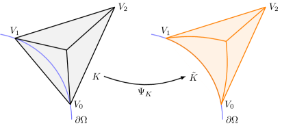
Figure 1. Barycentric refined element at the boundary of the domain (left) and corresponding curved element (right).

We have chosen two classical examples with known exact solutions [36]. In them the material parameters used are the Young modulus $E$ and the Poisson ratio $\nu$. They are related to the Lamé parameters by

(8.3) $$\lambda=\frac{E\nu}{(1+\nu)(1-2\nu)},\quad\textrm{and}\quad\mu=\frac{E}{2(1+\nu)}.$$

The incompressible limit is obtained for $\nu\to\frac{1}{2}$. The exact solutions are given in polar coordinates $r$ and $\theta$. In the expressions for the exact solutions the parameter value is $\kappa=3-4\nu$.

8.1. Circular hole in an infinite plate

The problem is that of the unstressed circular hole with radius $a$ in an infinite plate subject to the unidirectional tension $\sigma_{\infty}$ as discussed in Section 19.3.1 in [36]. The exact displacement is

$$u_{x} =\frac{\sigma_{\infty}a}{8\mu}\left(\frac{r}{a}(\kappa+1)\cos(\theta)+2\frac{a}{r}((1+\kappa)\cos(\theta)+\cos(3\theta))-2\frac{a^{3}}{r^{3}}\cos(3\theta)\right),$$

$$u_{y} =\frac{\sigma_{\infty}a}{8\mu}\left(\frac{r}{a}(\kappa-3)\sin(\theta)+2\frac{a}{r}((1-\kappa)\sin(\theta)+\sin(3\theta))-2\frac{a^{3}}{r^{3}}\sin(3\theta)\right),$$

and the exact stress components are given by

(8.4) $$\sigma_{xx} =\sigma_{\infty}\left(1-\frac{a^{2}}{r^{2}}(\frac{3}{2}\cos(2\theta)+\cos(4\theta))+\frac{3}{2}\frac{a^{4}}{r^{4}}\cos(4\theta)\right),$$

$$\sigma_{yy} =\sigma_{\infty}\left(-\frac{a^{2}}{r^{2}}(\frac{1}{2}\cos(2\theta)-\cos(4\theta))-\frac{3}{2}\frac{a^{4}}{r^{4}}\cos(4\theta)\right),$$

$$\sigma_{xy} =\sigma_{\infty}\left(-\frac{a^{2}}{r^{2}}(\frac{1}{2}\sin(2\theta)+\sin(4\theta))+\frac{3}{2}\frac{a^{4}}{r^{4}}\sin(4\theta)\right).$$

The computations we do for the domain $\Omega=(-b,b)\times(-w,w)\setminus\Omega_{\circ}$ with the hole given by $\Omega_{\circ}=\{(x,y)\in\mathbb{R}^{2}:|(x,y)|\leq a\}$, see the left picture of Figure 2.

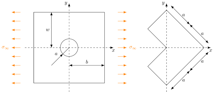
Figure 2. Computational domain for example 8.1 on the left and for example 8.2 on the right.

We choose $a=1$ and $b=w=4a$, and use the material parameters $E=1$ and $\nu=0.3,0.4,0.49,0.49999$. On the outer boundary we assign the traction obtained from (8.4) with $\sigma_{\infty}=1$. The displacement is fixed to be orthogonal to the rigid body motions.

Figure 3. Displacement components $u_{x}$ and $u_{y}$ of the solution of example 8.1

Figure 4. Stress components $\sigma_{xx}$, $\sigma_{xy}$ and $\sigma_{yy}$ of the solution of example 8.1

To validate the theoretical findings we introduce the relative $L^{2}$-error of the stress and strain

(8.5) $$e_{0}^{\sigma}=\frac{\|\sigma-\sigma_{h}\|_{0}}{\|\sigma\|_{0}},\quad\quad e_{0}^{u}=\frac{\|\varepsilon(u)-\varepsilon(u_{h}^{a})\|_{0}}{{\|\varepsilon(u)\|_{0}}},$$

for which the a priori estimates of Theorems 3 and 4, and the a posteriori estimate of Theorem 7 hold.

The second set of error quantities are the relative errors in strain energy for the stress directly obtained from the method, and computed from the displacement $u_{h}^{a}$, through (7.1)

(8.6) $$e_{\mathcal{C}}^{\sigma}=\frac{\|\sigma-\sigma_{h}\|_{\mathcal{C}}}{\|\sigma\|_{\mathcal{C}}},\quad\quad e_{\mathcal{C}}^{\mathcal{A}\varepsilon(u)}=\frac{\|\sigma-\mathcal{A}\varepsilon(u_{h}^{a})\|_{\mathcal{C}}}{\|\sigma\|_{\mathcal{C}}}.$$

The last set is those given by the hypercircle estimate

(8.7) $${e}^{\operatorname{mean}}_{\mathcal{C}}=\frac{\|\sigma-\frac{1}{2}(\sigma_{h}+\mathcal{A}\varepsilon(u_{h}^{a}))\|_{\mathcal{C}}}{\|\sigma\|_{\mathcal{C}}},\quad\quad c_{\operatorname{eff}}=\frac{\|\sigma-\frac{1}{2}(\sigma_{h}+\mathcal{A}\varepsilon(u_{h}^{a}))\|_{\mathcal{C}}}{\frac{1}{2}\|\sigma_{h}-\mathcal{A}\varepsilon(u_{h}^{a})\|_{\mathcal{C}}},$$

where $c_{\operatorname{eff}}$ measures the efficiency of estimate (6.8). The oscillation is a higher order term, and we expect that $c_{\operatorname{eff}}\rightarrow 1$ when $h\rightarrow 0$, which means that the error estimator is asymptotically exact. Further, we introduce the symbol $N$ for the number of elements in $\mathcal{C}_{h}$. For uniform refinements we have $h\sim N^{-1/2}$.

In Table 8.1 and Table 8.1 the errors and the order of convergence (oc) for the JM and the ADG method are given for varying Poisson ratios for a uniform mesh refinement. As predicted by the analysis all errors converge with optimal order $\mathcal{O}(N^{-1})$ and $\mathcal{O}(N^{-3/2})$, for JM and ADG, respectively, and the constant $c_{\operatorname{eff}}$ converges to $1$. Further, the quantities $e_{0}^{\sigma}$, $e_{0}^{u}$ and $e_{\mathcal{C}}^{\sigma}$ stay constant for all values $\nu$. Since in the incompressible limit $\nu\rightarrow\frac{1}{2}$, the Lamé parameter $\lambda\rightarrow\infty$, see (8.3), we expect that the errors, when computed from (7.1), should deteriorate. Indeed, although converging with optimal order, the errors ${e}^{\operatorname{mean}}_{\mathcal{C}}$ and $e_{\mathcal{C}}^{\mathcal{A}\varepsilon(u)}$ start to grow significantly in the incompressible limit. To give more insight on this behavior we have plotted in Figure 5 the error $e_{\mathcal{C}}^{\mathcal{A}\varepsilon(u)}$ for both methods with respect to the Poisson ratio. As we can see the blow up occurs continuously and can be made arbitrarily big if one approaches the incompressible limit.

We finally note that in all cases the stress $\sigma_{h}$ is much more accurate than that computed by ${\mathcal{A}}\varepsilon(u_{h}^{a})$. Furthermore, the latter dominates in ${e}^{\operatorname{mean}}_{\mathcal{C}}$, thus it holds ${e}^{\operatorname{mean}}_{\mathcal{C}}\sim\frac{1}{2}e_{\mathcal{C}}^{\mathcal{A}\varepsilon(u)}$, for all values of the Poisson ratio.

$N$	$e_{0}^{\sigma}$   ​(	oc   ​​​​)	$e_{0}^{u}$   ​(	oc   ​​​​)	$e_{\mathcal{C}}^{\sigma}$   ​(	oc   ​​​​)	$e_{\mathcal{C}}^{\mathcal{A}\varepsilon(u)}$   ​(	oc   ​​​​)	${e}^{\operatorname{mean}}_{\mathcal{C}}$   ​(	oc   ​​​​)	$c_{\operatorname{eff}}$
$\nu=0.3$
202	$0.042\,871\,596\,617\,184\,4$   ​(	–   ​​​​)	$0.109\,338\,535\,465\,414\,08$   ​(	–   ​​​​)	$0.042\,811\,380\,632\,161\,49$   ​(	–   ​​​​)	$0.119\,825\,444\,878\,047\,8$   ​(	–   ​​​​)	$0.063\,626\,449\,803\,328\,31$   ​(	–   ​​​​)	$0.941\,768\,951\,566\,39$
808	$0.018\,033\,372\,592\,435\,527$   ​(	$1.249\,352\,912\,657\,240\,7$   ​​​​)	$0.045\,318\,334\,727\,649\,48$   ​(	$1.270\,635\,202\,786\,904$   ​​​​)	$0.018\,005\,540\,554\,835\,213$   ​(	$1.249\,553\,449\,857\,585$   ​​​​)	$0.050\,014\,352\,192\,331\,72$   ​(	$1.260\,520\,238\,975\,607$   ​​​​)	$0.026\,587\,559\,894\,286\,853$   ​(	$1.258\,875\,246\,887\,115\,2$   ​​​​)	$0.941\,211\,404\,495\,277\,7$
3232	$0.004\,474\,325\,488\,659\,54$   ​(	$2.010\,927\,118\,697\,525\,7$   ​​​​)	$0.011\,833\,482\,457\,088\,705$   ​(	$1.937\,220\,144\,071\,597\,3$   ​​​​)	$0.004\,466\,693\,357\,059\,82$   ​(	$2.011\,161\,791\,463\,358\,4$   ​​​​)	$0.013\,176\,743\,868\,048\,943$   ​(	$1.924\,348\,245\,113\,595$   ​​​​)	$0.006\,958\,719\,377\,387\,909$   ​(	$1.933\,857\,643\,696\,277\,8$   ​​​​)	$0.947\,352\,628\,359\,106\,9$
12928	$0.001\,083\,670\,987\,859\,864\,3$   ​(	$2.045\,743\,402\,168\,842$   ​​​​)	$0.003\,254\,160\,158\,801\,607$   ​(	$1.862\,517\,542\,174\,591\,9$   ​​​​)	$0.001\,081\,726\,232\,730\,845$   ​(	$2.045\,871\,792\,819\,418\,6$   ​​​​)	$0.003\,626\,942\,704\,962\,359$   ​(	$1.861\,168\,046\,826\,081\,6$   ​​​​)	$0.001\,892\,858\,302\,822\,823\,8$   ​(	$1.878\,255\,412\,760\,195\,8$   ​​​​)	$0.958\,514\,996\,062\,917\,6$

$\nu=0.4$    202$0.042\,872\,271\,648\,751\,556$–$0.102\,475\,462\,123\,398\,9$–$0.042\,778\,759\,829\,114\,89$–$0.142\,507\,139\,379\,764\,64$–$0.074\,397\,126\,759\,434\,27$–$0.957\,807\,812\,720\,650\,4$ 808$0.018\,033\,450\,667\,146\,195$$1.249\,369\,382\,254\,343$$0.042\,844\,818\,820\,757\,004$$1.258\,085\,839\,573\,509\,5$$0.017\,990\,229\,280\,288\,07$$1.249\,681\,085\,447\,182$$0.060\,140\,245\,067\,192\,67$$1.244\,631\,545\,886\,565\,3$$0.031\,393\,922\,909\,917\,41$$1.244\,761\,589\,146\,047\,7$$0.958\,274\,153\,590\,215\,4$ 3232$0.004\,474\,325\,497\,171\,378$$2.010\,933\,362\,025\,560\,3$$0.011\,267\,054\,087\,642\,15$$1.927\,010\,397\,146\,157\,4$$0.004\,462\,472\,742\,087\,694\,6$$2.011\,298\,311\,504\,084$$0.016\,104\,283\,911\,148\,87$$1.900\,886\,235\,154\,05$$0.008\,357\,114\,977\,124\,548$$1.909\,408\,426\,226\,421\,3$$0.963\,865\,782\,945\,526\,9$ 12928$0.001\,083\,670\,987\,244\,913\,1$$2.045\,743\,405\,732\,073\,6$$0.003\,122\,456\,223\,471\,396\,4$$1.851\,357\,103\,488\,058$$0.001\,080\,650\,694\,478\,840\,2$$2.045\,943\,089\,790\,939$$0.004\,478\,028\,909\,150\,907$$1.846\,508\,764\,599\,818\,4$$0.002\,303\,611\,249\,235\,516\,5$$1.859\,107\,712\,302\,050\,3$$0.972\,231\,044\,110\,236\,2$    $\nu=0.49$    202$0.042\,873\,059\,416\,813\,53$–$0.093\,514\,042\,609\,256\,69$–$0.042\,738\,571\,987\,939\,095$–$0.378\,082\,324\,242\,212\,6$–$0.190\,245\,310\,890\,874\,24$–$0.993\,672\,494\,986\,657\,1$ 808$0.018\,033\,563\,210\,231\,05$$1.249\,386\,887\,660\,841\,2$$0.039\,573\,528\,443\,531\,01$$1.240\,647\,320\,491\,163\,2$$0.017\,971\,402\,778\,475\,608$$1.249\,835\,679\,972\,707$$0.161\,761\,625\,334\,636\,64$$1.224\,831\,005\,133\,050\,4$$0.081\,380\,954\,590\,749\,97$$1.225\,097\,786\,756\,948$$0.993\,916\,006\,984\,362\,3$ 3232$0.004\,474\,325\,510\,196\,897$$2.010\,942\,361\,362\,822\,3$$0.010\,513\,160\,504\,862\,775$$1.912\,339\,261\,426\,521\,3$$0.004\,457\,278\,086\,909\,669$$2.011\,468\,146\,710\,295\,3$$0.044\,458\,598\,939\,629\,355$$1.863\,335\,008\,855\,065\,5$$0.022\,341\,227\,773\,450\,486$$1.864\,982\,731\,150\,467\,4$$0.995\,033\,658\,419\,149\,6$ 12928$0.001\,083\,670\,986\,448\,385$$2.045\,743\,410\,992\,424$$0.002\,946\,598\,512\,643\,348\,7$$1.835\,074\,037\,528\,582\,3$$0.001\,079\,326\,868\,418\,410\,6$$2.046\,031\,129\,097\,716\,7$$0.012\,564\,366\,691\,074\,882$$1.823\,124\,530\,471\,139\,2$$0.006\,305\,417\,433\,904\,284$$1.825\,044\,683\,300\,798\,5$$0.996\,345\,912\,271\,747\,5$    $\nu=0.49999$    202$0.042\,873\,157\,839\,660\,82$–$0.092\,384\,036\,149\,877\,71$–$0.042\,733\,225\,441\,884\,68$–$11.711\,628\,690\,648\,638$–$5.855\,853\,329\,120\,688$–$0.999\,993\,343\,730\,304\,4$ 808$0.018\,033\,579\,228\,177\,846$$1.249\,388\,918\,179\,897\,2$$0.039\,159\,071\,313\,996\,624$$1.238\,297\,026\,433\,541\,3$$0.017\,968\,902\,087\,827\,816$$1.249\,855\,951\,768\,403\,6$$5.019\,426\,143\,745\,607$$1.222\,347\,380\,150\,613\,5$$2.509\,729\,234\,178\,312\,4$$1.222\,347\,693\,759\,295\,9$$0.999\,993\,624\,501\,338\,7$ 3232$0.004\,474\,325\,512\,115\,43$$2.010\,943\,642\,188\,256$$0.010\,417\,929\,465\,367\,768$$1.910\,277\,976\,317\,842\,6$$0.004\,456\,587\,754\,570\,699$$2.011\,490\,842\,526\,954$$1.384\,901\,260\,365\,951\,4$$1.857\,739\,314\,745\,269\,7$$0.692\,454\,230\,879\,004\,8$$1.857\,741\,103\,633\,349\,3$$0.999\,994\,844\,575\,019$ 12928$0.001\,083\,670\,986\,340\,952\,4$$2.045\,743\,411\,754\,058\,3$$0.002\,924\,419\,570\,667\,268\,4$$1.832\,846\,357\,683\,954\,4$$0.001\,079\,150\,935\,347\,829\,2$$2.046\,042\,852\,900\,644\,7$$0.392\,291\,188\,410\,034\,35$$1.819\,786\,284\,493\,395\,2$$0.196\,146\,339\,393\,917\,2$$1.819\,788\,305\,367\,809\,9$$0.999\,996\,231\,780\,357\,1$

Table 1. Errors and order of convergence for the hole in an infinite plate example 8.1 for the JM method and varying Poisson ratios $\nu$.

$\nu=0.4$    202$0.009\,935\,449\,820\,564\,596$–$0.023\,737\,759\,158\,593\,524$–$0.009\,912\,907\,203\,510\,467$–$0.033\,488\,377\,942\,044\,51$–$0.017\,465\,861\,015\,168\,487$–$0.959\,064\,638\,005\,015\,5$ 808$0.002\,704\,842\,957\,521\,581$$1.877\,040\,451\,980\,981$$0.010\,404\,140\,660\,066\,06$$1.190\,025\,941\,962\,208\,8$$0.002\,697\,655\,218\,435\,835$$1.877\,602\,252\,932\,247\,8$$0.015\,711\,365\,248\,640\,613$$1.091\,851\,948\,776\,428\,7$$0.007\,970\,971\,723\,439\,794$$1.131\,710\,249\,280\,082\,8$$0.985\,618\,675\,921\,750\,5$ 3232$0.000\,336\,135\,337\,530\,268\,05$$3.008\,430\,709\,345\,095\,3$$0.001\,316\,687\,281\,769\,961\,5$$2.982\,173\,163\,380\,334\,6$$0.000\,335\,207\,514\,241\,333\,4$$3.008\,579\,577\,336\,805$$0.001\,992\,587\,921\,577\,137\,6$$2.979\,093\,261\,279\,083\,5$$0.001\,010\,318\,018\,338\,904\,2$$2.979\,946\,128\,334\,281$$0.986\,167\,301\,191\,906\,4$ 12928$4.014\,130\,489\,544\,717\text{\!\cdot}{10}^{-05}$$3.065\,882\,798\,471\,533\,6$$0.000\,165\,413\,728\,268\,897\,98$$2.992\,761\,861\,784\,363\,7$$4.002\,784\,914\,377\,222\,5\text{\!\cdot}{10}^{-05}$$3.065\,978\,488\,687\,041$$0.000\,245\,922\,876\,501\,648\,2$$3.018\,365\,533\,335\,775\,3$$0.000\,124\,581\,199\,948\,133\,05$$3.019\,651\,203\,800\,438\,4$$0.987\,023\,968\,861\,833\,1$    $\nu=0.49$    202$0.009\,935\,450\,764\,379\,442$–$0.021\,959\,584\,901\,966\,978$–$0.009\,903\,025\,117\,450\,4$–$0.089\,771\,403\,841\,207\,5$–$0.045\,159\,489\,113\,974\,05$–$0.994\,003\,491\,737\,657\,2$ 808$0.002\,704\,842\,986\,813\,413$$1.877\,040\,573\,405\,799\,3$$0.009\,187\,894\,277\,108\,912$$1.257\,044\,622\,420\,407\,7$$0.002\,694\,504\,969\,583\,733\,5$$1.877\,849\,050\,902\,566\,5$$0.041\,610\,419\,323\,931\,37$$1.109\,311\,128\,988\,937$$0.020\,848\,923\,299\,290\,99$$1.115\,056\,284\,588\,737\,3$$0.997\,916\,548\,186\,190\,5$ 3232$0.000\,336\,135\,338\,187\,253\,75$$3.008\,430\,722\,148\,833\,3$$0.001\,165\,017\,176\,210\,281$$2.979\,383\,030\,928\,584$$0.000\,334\,800\,846\,163\,316\,83$$3.008\,645\,168\,330\,753\,4$$0.005\,285\,753\,960\,651\,359\,5$$2.976\,763\,649\,427\,321\,3$$0.002\,648\,183\,569\,607\,305$$2.976\,897\,843\,515\,610\,4$$0.998\,003\,907\,769\,439\,4$ 12928$4.014\,023\,401\,294\,103\text{\!\cdot}{10}^{-05}$$3.065\,921\,289\,763\,317\,2$$0.000\,136\,461\,402\,879\,544\,58$$3.093\,786\,367\,036\,857$$3.997\,674\,349\,995\,051\,5\text{\!\cdot}{10}^{-05}$$3.066\,070\,313\,865\,968$$0.000\,611\,574\,985\,046\,709\,2$$3.111\,507\,969\,332\,853$$0.000\,306\,440\,848\,356\,021\,9$$3.111\,322\,606\,423\,099$$0.997\,872\,894\,475\,569\,6$    $\nu=0.49999$    202$0.009\,935\,451\,030\,417\,826$–$0.021\,724\,837\,886\,751\,825$–$0.009\,901\,711\,843\,999\,371$–$2.781\,554\,647\,699\,758$–$1.390\,786\,185\,248\,031\,7$–$0.999\,993\,699\,617\,186\,4$ 808$0.002\,704\,842\,993\,357\,33$$1.877\,040\,608\,546\,021\,4$$0.009\,034\,812\,938\,879\,824$$1.265\,778\,775\,264\,409$$0.002\,694\,086\,320\,615\,882\,4$$1.877\,881\,888\,517\,783\,3$$1.287\,648\,763\,691\,361\,2$$1.111\,152\,331\,410\,381\,5$$0.643\,825\,795\,545\,412\,5$$1.111\,158\,355\,731\,009\,4$$0.999\,997\,818\,273\,815\,3$ 3232$0.000\,336\,135\,338\,325\,845\,9$$3.008\,430\,725\,044\,355$$0.001\,145\,873\,390\,242\,555\,4$$2.979\,047\,084\,398\,344$$0.000\,334\,746\,801\,338\,741\,86$$3.008\,653\,901\,502\,692\,3$$0.163\,588\,340\,274\,855\,1$$2.976\,597\,289\,043\,005$$0.081\,794\,341\,720\,815\,23$$2.976\,597\,430\,482\,756$$0.999\,997\,910\,511\,553$ 12928$4.014\,024\,034\,205\,332\text{\!\cdot}{10}^{-05}$$3.065\,921\,062\,881\,201$$0.000\,165\,314\,326\,176\,403\,3$$2.793\,163\,987\,312\,780\,3$$3.997\,012\,786\,389\,718\text{\!\cdot}{10}^{-05}$$3.066\,076\,176\,953\,594$$0.023\,689\,984\,670\,187\,007$$2.787\,720\,754\,031\,453$$0.011\,845\,009\,215\,522\,765$$2.787\,721\,724\,436\,777$$0.999\,998\,578\,416\,306\,2$

Table 2. Errors and order of convergence for the hole in an infinite plate Example 8.1 for the ADG method and varying Poisson ratios $\nu$.

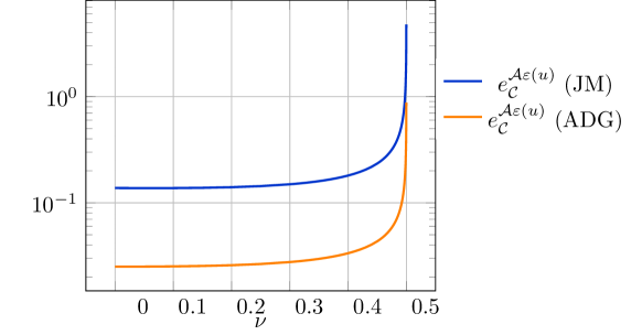
Figure 5. The error $e_{\mathcal{C}}^{\mathcal{A}\varepsilon(u)}$ of the JM and ADG method for the hole in an infinite plate example 8.1 for varying Poisson ratios on a fixed mesh with $N=606$

8.2. L-shape example

We employ an adaptive mesh refinement for the L-shape example from Section 10.3.2 of [36]. To this end let $\Omega$ be given by

$$\Omega=\{(x,y):|x|+|y|\leq{2}^{1/2}a\}\setminus\{(x,y):|x-2^{-1/2}a|+|y|\leq 2^{-1/2}a\},$$

as illustrated in the right picture of Figure 2. For our test case we choose $a=1$ and use $E=1$ and different values of $\nu$. Further, we define the constants $\alpha=0.544483737$ and $Q=0.543075579$. The exact displacement field, up to rigid-body displacements and rotations, is given by

$$u_{x} =\frac{1}{2\mu}r^{\alpha}((\kappa-Q(\alpha+1))\cos(\alpha\theta)-\alpha\cos((\alpha-2)\theta)),$$

$$u_{y} =\frac{1}{2\mu}r^{\alpha}((\kappa+Q(\alpha+1))\sin(\alpha\theta)+\alpha\sin((\alpha-2)\theta)),$$

and the stress components are

$$\sigma_{xx} =\alpha r^{\alpha-1}((2-Q(\alpha+1))\cos((\alpha-1)\theta)-(\alpha-1)\cos((\alpha-3)\theta)),$$

$$\sigma_{yy} =\alpha r^{\alpha-1}((2+Q(\alpha+1))\cos((\alpha-1)\theta)+(\alpha-1)\cos((\alpha-3)\theta)),$$

$$\sigma_{xy} =\alpha r^{\alpha-1}((\alpha-1)\sin((\alpha-3)\theta)+Q(\alpha+1)\sin((\alpha-1)\theta)).$$

To solve the problem we again enforce traction boundary conditions on the whole boundary $\partial\Omega$. We consider a uniform refinement and adaptive refinements where we use the a posteriori error estimator of Theorem 6 and for the incompressible limit the estimator given in Theorem 7. Now let $K\in{\mathcal{C}}_{h}$ be an arbitrary element, then we define the local contributions

$$\eta(K)^{2}=\frac{1}{4}\|\sigma_{h}-\mathcal{A}\varepsilon(u_{h}^{a})\|_{\mathcal{C},K}^{2}\quad\textrm{and}\quad\eta^{\operatorname{inc}}(K)^{2}=\mu^{1/2}\|\mathcal{C}\sigma_{h}-\varepsilon(u_{h}^{a})\|_{0,K}^{2},$$

where $\|\cdot\|_{\mathcal{C},K}$ reads as the norm $\|\cdot\|_{\mathcal{C}}$ restricted on the element $K$. The adaptive mesh refinement loop is defined as usual by

$$\mathrm{SOLVE}\rightarrow\mathrm{ESTIMATE}\rightarrow\mathrm{MARK}\rightarrow\mathrm{REFINE}\rightarrow\mathrm{SOLVE}\rightarrow\ldots$$

In the marking step we mark an element $K\in{\mathcal{C}}_{h}$ for refinement if $\eta(K)\geq\frac{1}{4}\max\limits_{K\in{\mathcal{C}}_{h}}\eta(K)$ or $\eta^{\operatorname{inc}}(K)\geq\frac{1}{4}\max\limits_{K\in{\mathcal{C}}_{h}}\eta^{\operatorname{inc}}(K)$. After that, the mesh refinement algorithm refines the marked elements plus further elements to guarantee a regular triangulation. Beside the error quantities introduced above we further define the (relative) estimators

$$\eta =\frac{\frac{1}{2}\|\sigma_{h}-\mathcal{A}\varepsilon(u_{h}^{a})\|_{\mathcal{C}}}{\|\sigma\|_{\mathcal{C}}},\quad \eta^{\operatorname{inc}} =\frac{\mu^{1/2}\|\mathcal{C}\sigma_{h}-\varepsilon(u_{h}^{a})\|_{0}}{\mu^{-1/2}\|\sigma\|_{0}},$$

and the scaled error e_0^u, inc =μ1/2∥ ε(u) - ε(uha) ∥0μ-1/2∥ σ∥0

In Figure 6 we plot the error history of $e_{\mathcal{C}}^{\sigma},\ e_{\mathcal{C}}^{\mathcal{A}\varepsilon(u)}$ and $e_{0}^{\operatorname{mean}}$ for the JM and the ADG method using an adaptive refinement based on the estimator $\eta$ for a moderate Poisson ratio $\nu=0.3$. From the coarsest to the finest mesh the measure of efficiency $c_{\operatorname{eff}}$ varies in in the range $0.99-1.00$, and hence the error estimator $\eta$ is not plotted as it would be indistinguishable from $e_{0}^{\operatorname{mean}}$. From the figure we see that all errors converge with optimal order $\mathcal{O}(N^{-(k+1)/2})$.

To show the drastic decrease of the errors when using an adaptive algorithm, we also include the error $e_{\mathcal{C}}^{\sigma}$ for a uniform refinement. Since the exact solution is in the Sobolev space $H^{s}$, with $s<1.54$, a uniform mesh only yields a convergence rate of ${\mathcal{O}}(h^{0.54})$, i.e. ${\mathcal{O}}(N^{-0.27})$.

In Figure 7 we plot the same quantities but using an incompressible setting with $\nu=0.49999$. Although all quantities still converge with an optimal order, we observe the same error deterioration as in the previous example. Thus, while $e_{\mathcal{C}}^{\sigma}$ (and also $e_{0}^{\sigma}$, $e_{0}^{u}$ which are not plotted) is not affected by the choice of the Poisson ratio $\nu$, the errors ${e}^{\operatorname{mean}}_{\mathcal{C}}$ and $e_{\mathcal{C}}^{\mathcal{A}\varepsilon(u)}$ and the estimator $\eta$ are much bigger and should not be used in practice.

To this end we follow the theory of Theorem 7, i.e. we employ the estimator $\eta^{{\operatorname{inc}}}$. In Figure 8 the corresponding relative errors and the estimator are plotted and we observe that (up to an unknown constant $\mathcal{O}(1)$) the error estimator gives a good prediction of the errors $e_{0}^{\sigma}$ and $e_{0}^{u,\operatorname{inc}}$. Further, all errors converge with optimal error $\mathcal{O}(N^{-(k+1)/2})$, $k=1,2$. Again we include the errors for a uniform refinement which shows the drastic decrease when using an adaptive algorithm.

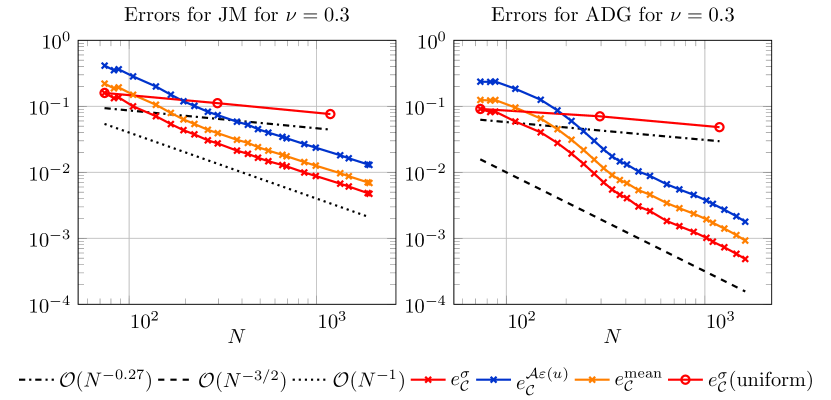
Figure 6. Error of the JM and ADG for the L-shape example 8.2 with an adaptive refinement using estimator $\eta$ and a constant Poisson ratio $\nu=0.3$.

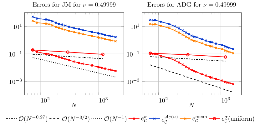
Figure 7. Error of the JM and ADG for the L-shape example 8.2 with an adaptive refinement using estimator $\eta$ and a constant Poisson ratio $\nu=0.49999$.

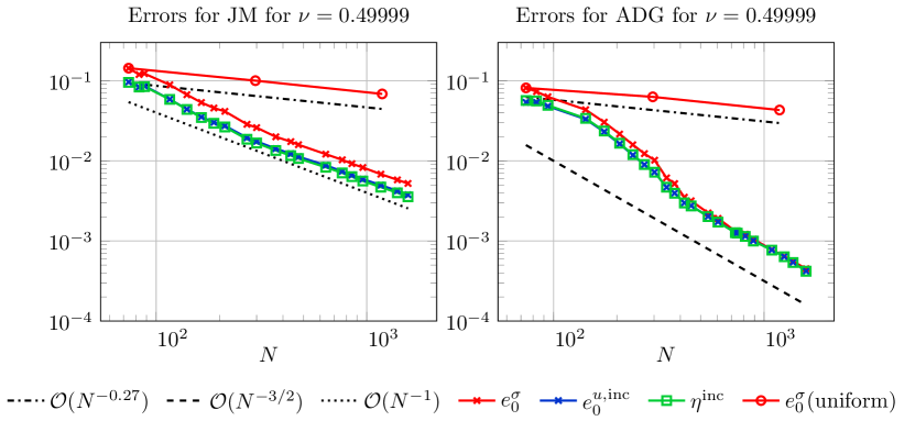
Figure 8. Error of the JM and ADG for the L-shape example 8.2 with an adaptive refinement using estimator $\eta^{\operatorname{inc}}$ and a constant Poisson ratio $\nu=0.49999$.

References

- [1] Douglas N. Arnold. An interior penalty finite element method with discontinuous elements. SIAM J. Numer. Anal., 19(4):742–760, 1982.
- [2] Douglas N. Arnold, Gerard Awanou, and Ragnar Winther. Finite elements for symmetric tensors in three dimensions. Math. Comp., 77(263):1229–1251, 2008.
- [3] Douglas N. Arnold and Franco Brezzi. Mixed and nonconforming finite element methods: implementation, postprocessing and error estimates. RAIRO Modél. Math. Anal. Numér., 19(1):7–32, 1985.
- [4] Douglas N. Arnold, Jim Douglas, Jr., and Chaitan P. Gupta. A family of higher order mixed finite element methods for plane elasticity. Numer. Math., 45(1):1–22, 1984.
- [5] Douglas N. Arnold, Richard S. Falk, and Ragnar Winther. Finite element exterior calculus, homological techniques, and applications. Acta Numer., 15:1–155, 2006.
- [6] Ivo Babuška, John Osborn, and Juhani Pitkäranta. Analysis of mixed methods using mesh dependent norms. Math. Comp., 35(152):1039–1062, 1980.
- [7] Ivo Babuška and Manil Suri. Locking effects in the finite element approximation of elasticity problems. Numer. Math., 62(4):439–463, 1992.
- [8] Garth A. Baker. Finite element methods for elliptic equations using nonconforming elements. Math. Comp., 31(137):45–59, 1977.
- [9] Christine Bernardi. Optimal finite-element interpolation on curved domains. SIAM Journal on Numerical Analysis, 26(5):1212–1240, 1989.
- [10] Fleurianne Bertrand and Gerhard Starke. Parametric raviart–thomas elements for mixed methods on domains with curved surfaces. SIAM Journal on Numerical Analysis, 54(6):3648–3667, 2016.
- [11] Raymond L. Bisplinghoff, James W. Mar, and Theodore H. H. Pian. Statics of deformable solids. Dover Publications, Inc., New York, 1990. Corrected reprint of the 1965 original.
- [12] Daniele Boffi, Franco Brezzi, and Michel Fortin. Mixed finite element methods and applications, volume 44 of Springer Series in Computational Mathematics. Springer, Heidelberg, 2013.
- [13] Susanne C. Brenner. Korn’s inequalities for piecewise vector fields. Math. Comp., 73(247):1067–1087, 2004.
- [14] Richard Courant and David Hilbert. Methods of mathematical physics. Vol. I. Interscience Publishers, Inc., New York, N.Y., 1953.
- [15] Daniele Antonio Di Pietro and Alexandre Ern. Mathematical aspects of discontinuous Galerkin methods, volume 69 of Mathématiques & Applications (Berlin) [Mathematics & Applications]. Springer, Heidelberg, 2012.
- [16] Jim Douglas, Jr. and Todd Dupont. Interior penalty procedures for elliptic and parabolic Galerkin methods. In Computing methods in applied sciences (Second Internat. Sympos., Versailles, 1975), pages 207–216. Lecture Notes in Phys., Vol. 58. 1976.
- [17] Baudouin M. Fraejis de Veubeke. Displacement and equilibrium models in the finite element method. In O.C Zienkiewics and G.S. Holister, editors, Stress analysis, pages 145–197. Wiley, 1965.
- [18] Kurt O. Friedrichs. Ein Verfahren der Variationsrechnung, das Minimum eines Integrals als das Maximum eines anderen Ausdruckes darzustellen. Nachrichten von der Gesellschaft der Wissenschaften zu Göttingen, Mathematisch-Physikalische Klasse, pages 13–20, 1929.
- [19] Vivette Girault and Pierre-Arnaud Raviart. Finite element methods for Navier-Stokes equations, volume 5 of Springer Series in Computational Mathematics. Springer-Verlag, Berlin, 1986. Theory and algorithms.
- [20] Thirupathi Gudi. A new error analysis for discontinuous finite element methods for linear elliptic problems. Math. Comp., 79(272):2169–2189, 2010.
- [21] Johnny Guzmán and Michael Neilan. Symmetric and conforming mixed finite elements for plane elasticity using rational bubble functions. Numer. Math., 126(1):153–171, 2014.
- [22] Antti Hannukainen, Rolf Stenberg, and Martin Vohralík. A unified framework for a posteriori error estimation for the Stokes problem. Numer. Math., 122(4):725–769, 2012.
- [23] Claes Johnson and Bertrand Mercier. Some equilibrium finite element methods for two-dimensional elasticity problems. Numer. Math., 30(1):103–116, 1978.
- [24] Ohannes A. Karakashian and Frederic Pascal. A posteriori error estimates for a discontinuous Galerkin approximation of second-order elliptic problems. SIAM J. Numer. Anal., 41(6):2374–2399, 2003.
- [25] P.L. Lederer and R. Stenberg. Analysis of weakly symmetric mixed finite elements for elasticity. In preparation.
- [26] Carlo Lovadina and Rolf Stenberg. Energy norm a posteriori error estimates for mixed finite element methods. Math. Comp., 75(256):1659–1674 (electronic), 2006.
- [27] Jindřich Nečas and Ivan Hlaváček. Mathematical theory of elastic and elasto-plastic bodies: an introduction, volume 3 of Studies in Applied Mechanics. Elsevier Scientific Publishing Co., Amsterdam-New York, 1980.
- [28] J. Pitkäranta and R. Stenberg. Analysis of some mixed finite element methods for plane elasticity equations. Math. Comp., 41(164):399–423, 1983.
- [29] W. Prager and J. L. Synge. Approximations in elasticity based on the concept of function space. Quart. Appl. Math., 5:241–269, 1947.
- [30] P.-A. Raviart and J. M. Thomas. A mixed finite element method for 2nd order elliptic problems. In Mathematical aspects of finite element methods (Proc. Conf., Consiglio Naz. delle Ricerche (C.N.R.), Rome, 1975), pages 292–315. Lecture Notes in Math., Vol. 606. Springer, Berlin, 1977.
- [31] J. Schöberl. NETGEN An advancing front 2D/3D-mesh generator based on abstract rules. Computing and Visualization in Science, 1(1):41–52, 1997.
- [32] L. R. Scott and M. Vogelius. Norm estimates for a maximal right inverse of the divergence operator in spaces of piecewise polynomials. RAIRO Modél. Math. Anal. Numér., 19(1):111–143, 1985.
- [33] Rolf Stenberg. On the construction of optimal mixed finite element methods for the linear elasticity problem. Numer. Math., 48(4):447–462, 1986.
- [34] Rolf Stenberg. Some new families of finite elements for the Stokes equations. Numer. Math., 56(8):827–838, 1990.
- [35] Rolf Stenberg. Postprocessing schemes for some mixed finite elements. RAIRO Modél. Math. Anal. Numér., 25(1):151–167, 1991.
- [36] B. A. Szabó and I. Babuška. Finite Element Analysis. A Wiley-Interscience publication. Wiley, 1991.
- [37] Rüdiger Verfürth. A posteriori error estimation techniques for finite element methods. Numerical Mathematics and Scientific Computation. Oxford University Press, Oxford, 2013.
- [38] V.B. Watwood and B.J. Hartz. An equilibrium stress field model for finite element solution of two-dimensional elastostatic problems. Internat. Jour. Solids and Structures, 4:857–873, 1968.