A comparative analysis of pulse time-of-arrival creation methods

Abstract

Context. Extracting precise pulse times of arrival (TOAs) and their uncertainties is the first and most fundamental step in high-precision pulsar timing. In the classical method, TOAs are derived from total intensity pulse profiles of pulsars via cross-correlation with an idealised ‘1D’ template of that profile. While a number of results have been presented in the literature relying on the ever increasing sensitivity of such pulsar timing experiments, there is no consensus on the most reliable methods for TOA creation and, more importantly, the associated TOA uncertainties for each scheme.

Aims. In this article, we present a comprehensive comparison of TOA determination practices, focusing on the creation of timing templates, TOA determination methods and the most useful TOA bandwidth. The aim is both to present a possible approach towards TOA optimisation as well as the (partial) identification of an optimal TOA-creation scheme and the demonstration of optimisation differences between pulsars and data sets.

Methods. We compare the values of data-derived template profiles as compared to analytic profiles and evaluate the three most commonly used template-matching methods. Finally, we study the relation between timing precision and TOA bandwidth to identify any potential breaks in that relationship. As a practical demonstration, we apply our selected methods to European Pulsar Timing Array data on the three test pulsars PSRs J0218+4232, J1713+0747 and J2145$-$0750.

Results. Our demonstration shows that data-derived and smoothed templates are typically preferred to some more commonly applied alternatives; the Fourier domain with Markov-chain Monte Carlo (FDM) template-matching method is generally superior to or competitive with other methods; and while the optimal TOA bandwidth is strongly dependent on pulsar brightness, telescope sensitivity and scintillation properties, some significant frequency averaging seems required for the data we investigated.

1 Introduction

Millisecond pulsars (MSPs, first discovered by Backer et al., 1982) are neutron stars which have been spun up or ”recycled” to rotation periods shorter than $\sim$30 ms through accretion of matter from a binary companion star (Alpar et al., 1982; Bhattacharya & van den Heuvel, 1991). Their extremely stable rotation periods make MSPs ideal laboratories to test a diversity of extreme astrophysical phenomena that cannot be accessed on Earth. Their applications include investigating turbulence and structures of the interstellar medium (Keith et al., 2013; Lam et al., 2018; Donner et al., 2019), testing relativistic gravity (Taylor & Weisberg, 1982; Archibald et al., 2018; Voisin et al., 2020), building a pulsar-based time standard (Hobbs et al., 2012, 2020), constraining masses in the Solar System (Champion et al., 2010; Caballero et al., 2018), measuring the magnetic field structure in the Galaxy (Han et al., 2018; Gentile et al., 2018) and detecting gravitational radiation (e.g.  Shannon et al., 2015; Lentati et al., 2016; Arzoumanian et al., 2020).

Detecting nanohertz gravitational waves (GWs) using pulsar timing is one of the main foci in pulsar-timing research at present (see the recent reviews by Tiburzi, 2018; Burke-Spolaor et al., 2019). It had been predicted (Jenet et al., 2005) that a detection can be achieved by monthly observations of 20 to 40 MSPs over five to ten years if these sources are characterised by white timing residuals with a root-mean-square (RMS) of $\sim 100$ ns. In order to achieve this ambition, three major Pulsar Timing Arrays (PTAs, see Foster & Backer, 1990; Romani, 1989) were constructed: the Parkes Pulsar Timing Array (PPTA, Manchester et al., 2013), the European Pulsar Timing Array (EPTA, Janssen et al., 2008; Desvignes et al., 2016) and the North-American Nanohertz Observatory for Gravitational waves (NANOGrav, Demorest et al., 2013). These three were subsequently combined in the International Pulsar Timing Array (IPTA, Verbiest et al., 2016; Perera et al., 2019). Even though substantial progress has been achieved in improving timing precision and sensitivity in subsequent data releases, both at the regional and global level, a detection has so far not been achieved, primarily due to two limiting factors. Firstly, even the most up-to-date and highest-quality data sets (like, e.g. the NANOGrav data set from Alam et al., 2021a, b) have too few pulsars with timing precision below or at the 100-ns level. Secondly, there are a number of corrupting effects, whose impact on timing precision requires careful consideration (Shannon & Cordes, 2012; Verbiest & Shaifullah, 2018). One example of recent progress in that regard, is the influence of the Solar-System Ephemerides, which was known to affect GW experiments (Tiburzi et al., 2016), but it was not properly taken into account until more recently (e.g.  Arzoumanian et al., 2018a; Vallisneri et al., 2020). Beyond this, several fundamental aspects of pulsar-timing analyses were identified as potential targets for optimisation and harmonisation efforts during the first global PTA data combination (Verbiest et al., 2016). Three particular recommendations from that work will be described below and investigated in detail throughout this paper.

Firstly, all standard pulsar-timing analyses are based on matching a so-called template or “standard” profile to the observations. There are, however, several different ways in which such template profiles can be constructed. As outlined by Lorimer & Kramer (2005), traditionally template profiles are constructed through addition of a large number of observations, thereby resulting in a pulse profile with a far higher signal-to-noise ratio (S/N) than any given observation. Such templates have the advantage that they by definition fully resemble the actual pulse shape, but the noise of the original observations is also contained in the template and hence may cause inaccurate correlations commonly referred to as “self-standarding” (Hotan et al., 2005). Three strategies have been devised to mitigate this issue: firstly, the template profile can be smoothed; secondly the template can be restricted to contain only the single brightest observation (which is then removed from the subsequent timing analysis and only used as template profile); and thirdly the template can be modelled with noise-free analytic functions (Lorimer & Kramer, 2005). As can be seen in, e.g. Desvignes et al. (2016); Demorest et al. (2013); Kerr et al. (2020) several of the above-mentioned approaches are presently in use, but no comprehensive comparison of the various template-creation options has been published.

Secondly, after a template profile has been created, the time-of-arrival (TOA) of a given observation is derived from the cross-correlation between the observation and the template. Traditionally this has been done in the Fourier domain, by fitting the phase-gradient of the cross-power spectrum of the template and the observation (Taylor, 1992), commonly referred to as the “Phase Gradient Scheme (PGS)” method. However, the standard implementation of this approach has often been found to report underestimated uncertainties. One suggested solution determines the TOAs in the same way, but derives the TOA uncertainties from a Monte Carlo analysis (referred to as the “FDM” method). This latter solution has been suggested (Verbiest et al., 2016) as being superior. Furthermore, Hotan et al. (2005) proposed a Gaussian-interpolation (“GIS”) cross-correlation algorithm (CCA) in the time-domain, which is supposedly better suited to low-S/N data sets. While recent pulsar-timing efforts have increasingly adopted the FDM method, usage of the PGS method is still widespread (Desvignes et al., 2016), in some cases (e.g.  Arzoumanian et al., 2015) with lower bounds imposed on the pulse S/Ns in order to avoid underestimation of TOA uncertainties. Here too a comprehensive, data-based (as opposed to simulation-based) comparative evaluation of the possible alternatives has so far not been undertaken.

Lastly, potential corruptions in the derived TOAs can arise from the usage of data-recording systems with large (${\gtrapprox}0.3$) fractional bandwidths (Verbiest & Shaifullah, 2018). This is particularly the case if the pulse-profile changes shape across the band and the scintillation bandwidth is of the same order as (or slightly smaller than) the observing bandwidth. Both of these conditions appear to be likely if the fractional bandwidth is large (Dai et al., 2015; Levin et al., 2016), causing the frequency-averaged profile shape to vary from one observation to the next. If the TOAs are derived from frequency-averaged observations and template, then the aforementioned variations will be reflected in the TOAs and in the TOA uncertainties, worsening the overall timing precision. One solution to this problem is to carry out two-dimensional template matching where both observation and template have frequency resolution and where in addition to the phase offset (or TOA) a frequency drift (or dispersion measure) is determined (Liu et al., 2014; Pennucci et al., 2014). An alternative solution is to derive multiple TOAs across the bandwidth of the observation (Demorest et al., 2013; Arzoumanian et al., 2015), either against a frequency-averaged template or through matching each channel of the observation against the corresponding channel in the template. In all of this, it is an unsolved question which TOA bandwidth would be optimal: too narrow a bandwidth would leave little signal and create TOAs that have high levels of radiometer noise, too wide a bandwidth and the scintillation effects risk becoming significant – the most useful TOA bandwidth is likely strongly pulsar dependent.

To date, PTAs either fully frequency averaged their TOAs (Desvignes et al., 2016), used timing-model extensions to correct for profile-shape variations (Arzoumanian et al., 2015) or have carried out a mixed approach where both frequency-averaged and frequency-resolved TOAs have been derived (Kerr et al., 2020).

The three detailed aspects of TOA creation outlined above are investigated in this paper. Specifically in Section 2 we introduce the data and pulsars we use to test and compare the aforementioned aspects of timing on these data; in Section 3 we describe the various analysis methods that were compared: template creation is discussed in Section 3.1, template matching methods in Section 3.2 and most useful TOA bandwidth determination in Section 3.3. Before carrying out the actual analysis on the real data, we run some simulations to evaluate the reliability of the TOA uncertainties derived by the various TOA determination methods. These simulations are presented in Section 4. We discuss our findings on the three test pulsars in Section 5 and summarise of our findings in Section 6.

2 Observations

Our analysis is based on data from the newest generation of data recorders at four of the radio telescopes that constitute the EPTA: the Effelsberg radio telescope (designated as “EFF”), the Jodrell Bank Lovell radio telescope (JBO), the Nançay decimetric radio telescope (NRT) and the Westerbork synthesis radio telescope (WSRT). Details on the observing systems used at each of these observatories are given below. The pulsars used for this initial investigation are PSRs J0218+4232, J1713+0747 and J2145$-$0750. These three pulsars were chosen because they represent a variety of characteristics. Specifically, PSR J1713+0747 is very bright, with a small duty cycle, and is one of the most precisely timed MSPs in PTAs. PSR J0218+4232 has a relatively high dispersion measure (DM), is fainter and consequently not as well timed. PSR J2145$-$0750 is in between the other two in terms of brightness and timing precision, but has a significantly longer spin period and appears to have more significant stochastic wide-band impulse-modulated self-noise (or SWIMS, Osłowski et al., 2011, commonly also known as pulse-phase jitter).

Some basic properties for these three pulsars are given in Table 1; the observatory-specific details of the observations used are given in Table LABEL:table:pulsae_parameter and the number and date ranges of the observations are given in Table 3.

In addition to the telescope-specific radio-frequency interference (RFI) mitigation strategies described below, all data were visually inspected through the software suite psrchive (Hotan et al., 2004; van Straten et al., 2012) before TOAs were derived as described in Section 3. Specifically, since the data near the edge of each sub-band are often corrupted by aliasing and spectral leakage problems, these channels are excised with the paz program.

Table 1: Basic parameters for the pulsars in our sample. Parameters are merely indicative and have been rounded. As an indication of the timing precision, the weighted RMS residual is quoted for the IPTA combination that provided the best timing precision for the given pulsar, rounded to one significant digit. ECORR refers to the mean “frequency-correlated EQUAD parameter” (Arzoumanian et al., 2014) and is a measure for the strength of SWIMS present in a given pulsar.

Parameter	J0218+4232	J1713+0747	J2145$-$0750	References
Period (ms)	2.3	4.6	16.1	Navarro et al. (1995); Foster et al. (1993); Bailes et al. (1994)
DM (cm/pc3)	61	16	9	Navarro et al. (1995); Foster et al. (1993); Bailes et al. (1994)
Orbital Period (days)	2.0	67.8	6.8	Desvignes et al. (2016); Arzoumanian et al. (2018b)
Flux density S1400 (mJy)	0.9	9.1	10.3	Kramer et al. (1998); Dai et al. (2015)
Pulse Width W50 (%)	43	2.4	2.1	Stairs et al. (1999); Manchester et al. (2013)
IPTA Timing RMS ($\mu$s)	7	0.2	1	Verbiest et al. (2016); Perera et al. (2019)
IPTA ECORR	–	0.16	1.3	Perera et al. (2019)

Table 2: Description of the observational set-up for the data used in this paper. Given are the telescope identifier (see text), the name of the data recording device (referred to as “backend”), the centre frequency $f_{\text{c}}$ of the observations, the observing bandwidth $BW$ (not considering RFI or band-edge removal), the number of frequency channels $N_{\text{chan}}$ and the maximum number of phase bins across the profile $N_{\text{bin}}$. Note that for some pulsars JBO and WSRT only had 256 phase bins, as specified in the text.

Telescope	Backend	$f_{\text{c}}$	$BW$	$N_{\text{chan}}$	$N_{\text{bin}}$
		(MHz)	(MHz)
EFF	PSRIX	1347.5	200	128	1024
JBO	Roach	1532	400	400 / 1600	2048
NRT	NUPPI	1484	512	128	2048
WSRT	PuMa II	1380	160	512	1024

Table 3: Summary of observations used in this paper. For each pulsar-telescope combination the number of observations $N_{\text{obs}}$, MJD range and observing time span $T$ is given.

PSR	Tel ID	$N_{\rm obs}$	MJD	$T$ (yrs)
J0218+4232	EFF	53	55600–57705	5.8
	JBO	128	55666–58559	7.9
	NRT	467	55854–58558	7.4
	WSRT	65	54775–57131	6.5
J1713+0747	EFF	96	55633–58713	8.4
	JBO	301	55905–58610	7.4
	NRT	368	55800–58558	7.6
	WSRT	112	54155–57195	8.3
J2145$-$0750	EFF	62	55633–57733	5.7
	JBO	122	55880–58495	7.2
	NRT	265	55803–58555	7.5
	WSRT	85	54520–57135	7.2

2.1 Effelsberg radio telescope

The Effelsberg radio telescope is a homological Gregorian design with a 100-m paraboloidal primary reflector and a 6.5-m ellipsoidal secondary reflector, which makes the Effelsberg radio telescope the world’s second-largest fully movable telescope. It operates at wavelengths from about 90 cm to 3.5 mm (i.e. observing frequencies from 300 MHz to 90 GHz).

The data from Effelsberg presented in this research were acquired with a typical cadence of 3–4 weeks between 2011 and 2019 with an integration time per source of about 30 min per observation. The data recorder (henceforth referred to as “backend”) used was the PSRIX pulsar-timing system (Lazarus et al., 2016), which is based on the Reconfigurable Open Architecture Computing Hardware (ROACH) boards and carries out coherent dedispersion on central processing units (CPUs) using the dspsr (van Straten & Bailes, 2011) package. The observations were taken with the P-217 and P-200 receivers, centred at 1.3475 GHz in a frequency-multiplexing mode where eight 25-MHz-wide subbands are independently dedispersed and written to disk. This results in observations with a total of 200 MHz of bandwidth, 128 frequency channels, 1024 phase bins, 10-second integrations and full polarisation information.

These data were combined in time and frequency with the psradd command of the psrchive package (Hotan et al., 2004; van Straten et al., 2012). Subsequently RFI was removed automatically with clean.py, the RFI excision script of the COASTGUARD package (Lazarus et al., 2016), using the “surgical” algorithm.

2.2 Lovell radio telescope

At Jodrell Bank Observatory the 76-m Lovell telescope is used in a regular pulsar-monitoring programme. The observations used in this work were taken from that programme, have a centre frequency of 1.532 GHz, a timespan of $\sim$7.5 years, a typical cadence of three weeks and a typical integration time of 15 minutes. For PSR J1713+0747 the cadence was closer to one week. The backend used for these observations was a ROACH-based backend very similar to the one used at the Effelsberg observatory and described by Lazarus et al. (2016), and using the dspsr package (van Straten & Bailes, 2011) for real-time coherent de-dispersion.

The JBO observations have a bandwidth of 400 MHz split over 25 16-MHz-wide subbands, each channelised into 1 or 0.25 MHz wide frequency channels. The number of phase bins varies between 256 and 2048 depending on the pulsar observed. For the data set we used in this work, PSR J0218+4232 has the minimum 256 bins.

To remove the RFI, the spectral kurtosis method for real-time RFI removal (Nita et al., 2007) was applied during the dspsr pre-processing, after which the data were run through some basic RFI-removal scripts and finally were visually inspected for excluding the remaining RFI.

2.3 Nançay decimetric radio telescope

Built in 1965, the Nançay decimetric radio telescope (NRT) is a Kraus-type telescope with a collecting area of 6912 m², equivalent to a 94-m parabolic dish. Since 2011, NRT observations of pulsars are done with the ROACH-based NUPPI backend (Cognard et al., 2013), a version of the Green Bank Ultimate Pulsar Processing Instrument (DuPlain et al., 2008) designed for Nançay. With a total bandwidth of 512 MHz, the NUPPI backend splits the full bandwidth into 128 channels, each channel with 4 MHz bandwidth. The observations used here were centred at 1484 MHz and were coherently dedispersed in real-time on GPU units that are part of the NUPPI system.

The pulsars were observed with NUPPI since 2011 with a cadence that varied between five and ten days and with an integration time between 45 and 60 minutes per observation. Various automated RFI excision schemes were applied in post-processing offline.

2.4 Westerbork synthesis radio telescope

The Westerbork synthesis radio telescope (WSRT), located in the Netherlands and operated by the Netherlands Institute for Radio Astronomy (ASTRON), is an east-west interferometric array with 14 25-m parabolic dishes, which in terms of collecting area is equivalent to a 94-m single telescope.

Pulsar monitoring at the WSRT has been carried out at 350 MHz, 1.38 GHz and 2.27 GHz with the Pulsar Machine II (PuMa-II) backend (Karuppusamy et al., 2008). Pulsar observations are recorded in eight 20-MHz-wide sub-bands, for a total observing bandwidth of 160 MHz with 512 ($=8\times 64$) frequency channels. Coherent dedispersion is performed offline with the dspsr package.

The observations used in this paper were taken at a centre frequency of 1380 MHz, had a cadence of roughly one month and a total integration time of about 30 minutes. For PSRs J0218+4232 and J1713+0747, data with only 256 bins were used in this work.

3 Data processing techniques

In this section we describe the different algorithms and methods we use and compare. Specifically, the template creation methods are described in Section 3.1, the template-matching methods are outlined in Section 3.2 and the analysis to determine the most useful TOA bandwidth is described in Section 3.3. All of these algorithms and methods make use of the psrchive and tempo2 (Hobbs et al., 2006) software packages.

3.1 Template creation and comparison

The ideal template describes the pulse profile shape in perfect detail, without additive noise. A vital and complicating aspect in this regard is the fact that the achievable timing precision for a given profile shape is a strong function of the higher-frequency components present in the profile shape, i.e. of sharp features in the profile (e.g.  van Straten, 2006). Consequently, depending on the pulsar in question, noise-mitigation methods like smoothing or modelling of template profiles may require particular care in order to prevent negative impacts on the timing potential of a given pulsar.

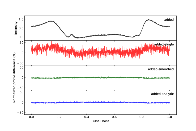
(a) PSR J0218+4232.

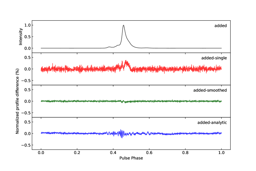
(b) PSR J1713+0747.

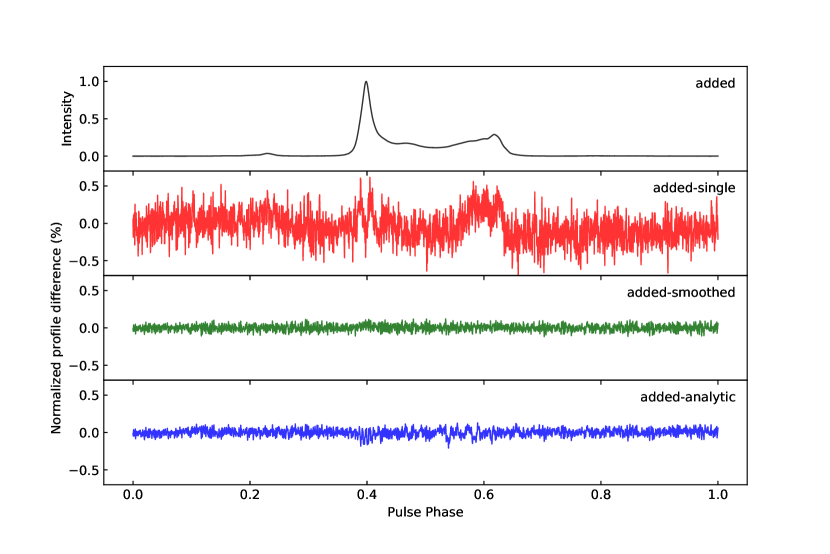
(c) PSR J2145$-$0750.

Figure 1: Peak-normalised added template profile and profile differences between the added and all other templates derived from NRT data. From top to bottom, shown are PSRs J0218+4232, J1713+0747, J2145$-$0750.

Common approaches towards template generation were already discussed in the introduction, thus here we summarise the four different methods we compare:

Single-brightest observation (henceforth “single”):

Here we take the observation with the highest S/N for use as a template and remove it from the observations to be timed. This approach has the advantage that all true features of the pulse profile are present in the template, but the disadvantages that the templates tend to have higher noise levels than in alternative approaches and are more susceptible to negative impacts from effects such as scintillation, profile evolution, SWIMS, and man-made extra noise such as mis-calibration or RFI. While this approach is convenient for pulsars that have large variations in S/N since the noise present in the template for such pulsars may be negligible in comparison to the noise present in the typical observation. However, in the case that the dataset is composed of a limited number of observations, it can be disadvantageous to exclude the most valuable (i.e. brightest) observation from the timing.

All observations added (henceforth “added”) :

The added template consists of all observations added together, while aligning them using the timing ephemeris of the data. The RFI and misaligned integrations due to, e.g. clock offsets are then zapped out. The cleaned archives are then re-weighted with several methods (S/N, S/N², off-pulse RMS) and the one with the highest resulting S/N is then chosen as the final added template. This approach also has the advantage that by definition all true profile features are present in the template; and particularly for pulsars with stable S/Ns the added template profile would have a much higher S/N than the single template. The main disadvantage is the risk of self-standarding (Hotan et al., 2005), which is due to the fact that noise in observations is correlated with their contributions in the template baseline. The impact of this effect is strongly dependent on the number of observations added into the template and on the S/N of the added observations (Hotan et al., 2005). Specifically, it has been found to be most relevant for pulsars in which the typical S/N is small (of order $\lesssim 25$) and in cases where less than several hundred observations are added together. The effect is also more problematic for strongly scintillating pulsars since the effective (i.e. S/N-weighted) number of added pulses tends to be smaller in this case.

Added with smoothing (henceforth “smoothed”):

Here the added profile is taken as a basis and a smoothing filter is applied subsequently. Specifically we used templates smoothed with the default wavelet-based smoothing algorithm of the psrchive/psrsmooth routine (Demorest et al., 2013), i.e. with an undecimated Daubechies wavelet with factor 8. The Daubechies wavelets are a family of orthogonal wavelets defining a discrete wavelet transform; the “undecimate” version of them is translation invariant; and the factor refers to the number of coefficients used (Daubechies, 1992). Limited testing with variations of the smoothing parameters and wavelets used indicated that these generally did not result in significantly different results for our analysis. The advantage of this approach is that the self-standarding issue should be removed as the noise in the template is largely suppressed, but this comes at the cost of a potential loss or suppression of sharp features in the pulse profile. An added complication is that smoothing algorithms can introduce artefacts in the template. The precise application of the smoothing algorithm could in itself be expanded to a far more extensive study, as results may also depend on the number of phase bins across a profile (i.e. the extent to which high-frequency profile features are resolved or not), but for the present work we restrict ourselves to the most standard application of this method, in order to limit the dimensionality of our analysis.

Analytic profile (henceforth “analytic”):

For this profile, von Mises functions (Jammalamadaka & Sengupta, 2001; Evans et al., 2001) were fitted to the added profile. Given the high S/N of the added profiles, dozens of components were typically required. Components were added and fitted interactively to avoid overfitting and to ensure as good a template profile as possible. This method has the clear advantage that the template profile is truly noise-free, but often not all sharp features may be represented in the profile, either because they are mis-identified as noise or because the analytic function cannot be indefinitely extended without affecting the stability and convergence of the least-squares fit. Consequently self-standarding is of no concern, but timing precision may be compromised.

An illustration of how the different methods compare is included in Figure 1 which shows the added templates derived from the NRT data for all three pulsars, as well as the profile differences comparing the added profile to the other three templates. As expected, the differences are mostly dominated by white noise, although the added-single difference does show coherent structure, in particular (though not exclusively) in the on-pulse phase range. This is likely caused by calibration issues, scintillation or low-level RFI. The added-analytic difference is far better behaved, but here too some non-white signals are visible, demonstrating the limitations of the von-Mises functions in modelling of pulse profile shapes. The added-smoothed difference is the closest to pure white noise for all three pulsars, indicating that the wavelet smoothing successfully manages to remove noise and keep structure. Nevertheless, even the smoothed template shows a minor deformation near the pulse peak of PSR J1713+0747. To what degree these discrepancies affect the timing of these pulsars, will be assessed in Section 5.1.

Note that throughout the presented work the aforementioned templates are used only in their frequency-averaged form, except for the analysis focused on the most useful TOA bandwidth, which was based on an added template that was not frequency averaged. A comparative analysis of frequency-resolved analytic templates (as developed by Liu et al., 2014; Pennucci et al., 2014) is deferred to a separate study, given the inherent complexity and multi-dimensional analysis necessary for such work.

3.2 TOA determination methods

After creation of a template profile, the TOA of a given observation can be determined by matching the observation to this template. Specifically, the observation $\mathcal{O}$ can be related to the template $\mathcal{T}$ as (Taylor, 1992):

$$\mathcal{O}\left(\phi\right)=a+b\mathcal{T}\left(\phi+\tau\right)+n\left(\phi\right),$$

where $\phi$ is the rotational phase, $a$ is an arbitrary offset, $b$ is a scale factor, $\tau$ is the phase offset between observation and template and $n\left(\phi\right)$ is a noise term. In order to solve for $\tau$, a variety of possible approaches have been proposed. We will compare three of the more commonly used methods, described briefly below.

Fourier phase gradient (PGS):

The most common template-matching method used to date (and the default method used in the psrchive software package) is the so-called PGS method described in detail by Taylor (1992). Based on the Fourier shift theorem, it matches the template to the observation by fitting for a slope in the Fourier space. A clear advantage of this approach is that the phase resolution does not impose a fundamental limit on the achievable measurement precision and as such can result in significantly more precise measurements than time-domain cross-correlation methods (which, according to Taylor, 1992, are limited to a precision about ten times smaller than the data’s resolution). The main disadvantage of this method is that in the low-S/N regime it underestimates the TOA uncertainty since the TOA distribution no longer follows a Gaussian distribution (see the discussion in Arzoumanian et al., 2015, Appendix B.).

Fourier domain with Markov-chain Monte Carlo (FDM):

One proposed solution to the underestimation of low-S/N TOA uncertainties is to probe the likelihood–phase shift dependence with a one-dimensional Markov-chain Monte Carlo, from which the TOA variance can be derived. This results in TOA values that are identical to those of the PGS method, but TOA uncertainties that are more realistic (i.e. larger), particularly for low-S/N observations.

Gaussian interpolation shift (GIS):

This algorithm carries out a standard cross-correlation of the template and observation in the time domain; and determines the phase offset by fitting a Gaussian to the cross-correlation function, whereby the centroid of the resulting Gaussian is defined as the TOA; the offset required to double the $\chi^{2}$ of the template-observation comparison is defined as the TOA uncertainty (Hotan et al., 2005). As mentioned above, this time-domain method has limited precision, but it was proposed as a more robust TOA determination method in the low-S/N regime.

The application of a Gaussian in determining the peak position of the cross-correlation function should result in timing precision exceeding 10% of a phase bin, although this likely depends on the exact pulse shape.

3.3 TOA bandwidth and SWIMS

The most significant contribution to the TOA uncertainty is referred to as radiometer noise. For a certain telescope, according to the radiometer equation (for details, please refer to Appendix 1 of Lorimer & Kramer, 2005), the radiometer noise, $\sigma_{\rm{rm}}$, scales with bandwidth $B$, integration time $T$ as,

$$\sigma_{\rm{rm}}\propto\frac{1}{\sqrt{TB}}.$$ (1)

In general, the sensitivity of pulsar timing would increase with the increase of observational bandwidth. However, as the TOA bandwidth increases, other noise sources become increasingly significant and the traditional approach of deriving TOAs from fully frequency-averaged observations can become increasingly complex, particularly if scintillation and profile evolution are significant.

At the other extreme, TOAs determined using native frequency resolution (referred to hereafter as “fully frequency-resolved TOAs”) significantly decreases the S/N, possibly leading to the low-S/N regime where some template-matching methods don’t provide reliable uncertainties anymore; in addition, TOAs at native frequency resolution can substantially increase the data volume and hence the computational cost of timing analyses, particularly for wideband systems. Consequently, there must be an most useful TOA bandwidth which maximises the TOA precision by limiting the deleterious effects of low S/N in fine frequency channels and those due to scintillation and profile evolution in frequency-averaged TOAs.

Here we have investigated such an most useful TOA bandwidth for a set of pulsar and backend combinations, by quantifying the achievable timing precision as a function of the TOA bandwidth. To do so, we combined the best template-matching method with a frequency-resolved version of the optimal template profile, and then carried out the timing of each pulsar and backend combination of our test dataset for a range of possible TOA bandwidths. This allowed us to investigate the improvement in the goodness of fit (of the timing model to the TOAs) via the reduced chi-squared of the linearised least-squares fit and the RMS of the timing residuals, as well as the number of TOAs that remain after removing TOAs corresponding to total intensity profiles with S/N less than 8, following Arzoumanian et al. (2015).

Radiometer noise is proportional to the square root of the TOA bandwidth and jitter noise or SWIMS (Osłowski et al., 2011; Cordes & Downs, 1985; Liu et al., 2012) behaves as a constant noise term, added in quadrature to the radiometer noise. The combined effect of profile evolution and scintillation strongly depends on the specific pulsar properties. Theoretically this effect should get stronger with larger TOA bandwidths, but given the relatively narrow bandwidth of our data, it is likely to behave somewhat differently. In addition, a number of systematic effects (e.g. calibration errors or instrumental artefacts; see Verbiest & Shaifullah, 2018, for a full review) are not expected to strongly depend on TOA bandwidth, although this would again be highly variable and dependent on the particular situation. In analysing the timing residual RMS as a function of TOA bandwidth, we consequently do not expect the straightforward scaling of the radiometer noise (Eq. 1), but expect a pulsar-dependent slope and likely some form of RMS saturation at the widest bandwidths – we will henceforth refer to the level of this RMS saturation as the “system limited noise floo” or SLNF. Consequently, we will quantify the residual RMS as a function of TOA bandwidth as follows:

$$\sigma_{\text{res}}=\sqrt{\frac{CB^{\alpha}}{T}+\sigma_{\text{NF}}^{2}},$$ (2)

where $\sigma_{\text{res}}$ is the residual RMS of the post-fit residuals, $C$ is a constant, $T$ is the integration time of the TOAs, $B$ is the bandwidth of the TOAs, $\alpha$ is a scaling index which would be $-1$ in the case of pure radiometer noise and $\sigma_{\text{NF}}$ is the SLNF, i.e. the part of the RMS that does not scale with TOA bandwidth. This last term is mostly expected to quantify the impact of SWIMS but also comprises other effects as described above. An example of this dependence is shown in Figure 2.

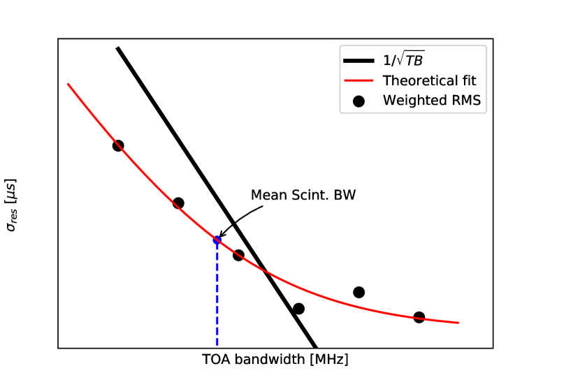
Figure 2: A sketch of the dependence of $\sigma_{\text{res}}$ on TOA bandwidth, for an idealised dataset. The black dots represent RMS values, the blue dashed line indicates the median scintillation bandwidth and the red line is a fit of Equation 2. The black line is for the case of pure radiometer noise, i.e. with no jitter or other corrupting noise sources ($\sigma_{\rm NF}=0$) and for standard scaling following the radiometer equation ($\alpha=-1$)

While the above considerations prevent a meaningful connection to the physical phenomenon of SWIMS, our analysis does allow a phenomenological determination of which TOA bandwidth optimally balances the various effects that impact the final timing RMS.

4 Simulations

Since the analysis on real data is complex and multi-faceted, we first carry out some relatively straightforward simulations to inform us on a few key points of the subsequent analysis. Specifically, we use simulations to study how the TOA uncertainties from the various TOA determination methods scale with pulse S/N; and to check to what degree these results depend on the pulse shape. Furthermore, since these tests depend on the S/N, which is being used to place a cut-off to remove unreliable TOAs (in accordance with the advice of Arzoumanian et al., 2015), we also evaluate how well the standard S/N algorithm of the psrchive package can reproduce the simulated S/N.

These simulations were written in python using the numpy package and psrchive through its python interface. Specifically, noise-free templates were constructed with the paas routine of psrchive, after which white noise with varying intensity was added to those profiles. Here we tested five profile shapes as shown in the inset plots of Figure 3: a simple Gaussian profile; a Gaussian profile with a sharp notch on its trailing edge; and finally the analytic profiles derived for each of our three test pulsars, based on the NCY data described earlier.

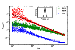
(a)

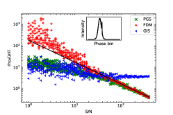
(b)

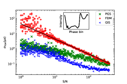
(c)

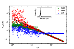
(d)

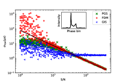
(e)

Figure 3: TOA uncertainty obtained from various noise-added profiles as a function of the simulated S/N. The top-left panel shows the results for a simple Gaussian profile, the top-right panel shows results for a Gaussian profile with a notch, and the bottom panels display the results for the analytic templates of PSRs J0218+4232, J1713+0747, and J2145$-$0750, respectively, as derived from NCY data. CCAs are shown with different colours and markers, as indicated in the legend. The black solid line in each panel is a fit to high-S/N (¿ 10) FDM data and is extended to low-S/N data. At each S/N plotted, ten simulations were run, although these are typically indistinguishable at high S/N. The inset within each panel shows the profile.

Ideally, according to the radiometer equation, the TOA uncertainty should follow an inverse relationship with S/N, in the form of: $\sigma\propto\frac{1}{S/N}$. From Figure 3, we can see that PGS and FDM are consistent with each other in most cases and follow this scaling in the high-S/N regime, although a minor deviation in the slope of the PGS curve can be identified for PSR J0218+4232. However, if the S/N is low, i.e. less than $\sim$10, the difference between FDM and PGS becomes more explicit, although the exact threshold S/N strongly depends on the pulse shape: for the complex profile shapes of PSRs J1713+0747 and J2145$-$0750 the curves coincide down to lower S/Ns; for the simple Gaussian or Gaussian-with-notch profiles the discrepancies are clearer even at S/N=10. These results clearly show that PGS typically underestimates the TOA uncertainties in the low-to-medium S/N regime, although the degree of underestimation strongly depends on the profile shape. In contrast, FDM displays a tendency to overestimate the TOA uncertainties in the same S/N regime, primarily for pulse profiles with sharp features.

It is furthermore evident that GIS fails to determine the uncertainty correctly in both the low-S/N and high-S/N regimes, except for a very narrow region. Similar to the results from Hotan et al. (2005), our simulations show that GIS works better at the low-S/N regime; and the range of good performance is wider for pulsars with a large duty cycle. Nevertheless, our simulations suggest the uncertainties are consistently underestimated, even at low S/Ns. This latter difference may be partly related to the S/N of the template used, which we made unrealistically large to more clearly demonstrate the trends independently of template; although clearly the complexity of the pulse profile shape also has a significant impact, as already anticipated by Hotan et al. (2005). For profiles with narrow features, our simulations for GIS show that the TOA uncertainty flattens off for S/Ns above a few tens, indicating significant overestimation of uncertainties for high-S/N observations.

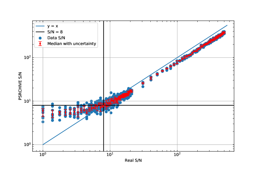
Figure 4: S/N determined with the standard implementation in psrchive as a function of simulated S/N. The blue points are the S/N of the individual simulations, while the red points indicate the median value of the simulations, the red error bars indicate the 25th and 75th percentiles at each real S/N. For this simulation, the analytic template based on NRT data of PSR J2145$-$0750 was used. Due to differences in the definition of the S/N, some inconsistencies between x and y values are expected, although the scaling should be linear, as is the case in the high-S/N regime. In the low S/N regime (S/N$<10$), the S/Ns returned by psrchive are typically overestimated and have a significant random component. (The thick black lines indicate S/Ns of 8, which is used as a S/N cut-off value in this work, following Arzoumanian et al. (2015).)

Figure 4 shows the results of our consistency check on the S/N values returned by psrchive. Since the exact S/N depends on the precise definition used as well as on the pulse shape, no exact equivalence can be expected between the simulations and the measurements, but a linear relationship should exist. Our results show that this linear relationship does indeed describe the majority of the simulated S/N range, but that this flattens off below a S/N of $\sim$10, where the S/N returned by psrchive is mostly unrelated to the actual S/N simulated. While the details of this figure – and particularly the scaling at high-S/N – differ between the various pulse profiles we tested, the flattening off below a S/N of ten is persistent.

A consequence of this test lies in the interpretation of Figure 3: while for some pulsars the TOA uncertainties from FDM and PGS appear reliable down to a S/N of approximately five, in practice it is not possible to reliably measure S/Ns below ten. Consequently, in order to reliably identify TOAs with reliable error bars, a cut-off at a S/N of about ten may be required in any case, which could cause any difference between PGS and FDM to become irrelevant for a wide range of pulse shapes. (In contrast, Figure 3(c) indicates that for pulse shapes with particularly large duty cycles differences may persist even above a S/N of ten.)

5 Results and discussion

To evaluate the timing precision as a function of the choice of template and CCA described in Sections 3.1 and 3.2, and to study the most useful TOA bandwidth as described in Section 3.3, we analysed the TOAs with the timing models presented by Desvignes et al. (2016) and Chen et al. (2021). For PSR J1713+0747 we adopted the entire timing model of Chen et al. (2021), including DM and red noise models. For PSRs J0218+4232 and J2145$-$0750 we used the timing models from Desvignes et al. (2016), but without inclusion of the red noise or DM models. In the timing models of Desvignes et al. (2016) the planetary ephemerides were updated to DE438 and the reference clock was updated to TT(BIPM2019).

5.1 Template and CCA

For each combination of the templates and CCAs described in Section 3, we performed a tempo2 (Edwards et al., 2006; Hobbs et al., 2006) analysis, fitting only for the pulsar spin and its first derivative. For each fit, the reduced $\chi^{2}$ and the residual RMS value were recorded, along with the resulting timing residuals.

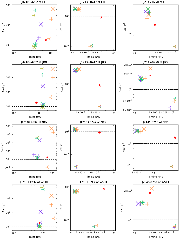
Figure 5: Reduced $\chi^{2}$ and residual RMS for the three pulsars as a function of the selected CCA and template and the different telescopes. The dashed line indicates a reduced $\chi^{2}$ of 1, and the red stars represent results from Desvignes et al. (2016)

Figure 5 presents a pulsar and telescope-wise analysis of the timing performance. Here the poor performance of the GIS TOAs is clearly visible, across all systems. Further, it is evident that FDM and PGS results often cluster for the two stronger sources, with generally almost identical reduced $\chi^{2}$ and RMS values, independent of the template creation method. This shows that the effect of template choice can be somewhat mitigated for such sources when these CCAs are used. Finally, for those cases where FDM and PGS do differ, FDM tends to outperform PGS, particularly in terms of the reduced $\chi^{2}$ values obtained.

In Figure 5, it is also noticeable that for faint pulsars like PSR J0218+4232, the high noise levels in the single template severely compromise the results. In this case, even the added template shows poor results when combined with the PGS method, indicating that some level of self-standarding (as described by Hotan et al., 2005) may be at work. However, the FDM method appears far more robust to this phenomenon.

The timing residuals for each of the TOA sets were further assessed to check for the presence of unmodelled signals or persistent outlier TOAs. Using a 2-tailed Kolmogorov-Smirnov test we compared the power spectrum of these residuals against a power spectrum consisting of purely Gaussian or power-law signals or a combination of both. We find that the power spectra of the timing residuals for all three pulsars are Gaussian or a Gaussian and power-law mixed distribution, suggesting that the updated timing models are sufficient given our data (i.e. the timing-model parameters that were not refitted model the TOAs sufficiently well that no clear timing signatures were present in the data). Visual inspection of the timing residuals confirms that the timing residuals of PSRs J0218+4232 and J2145$-$0750 are essentially white; the timing residuals of PSR J1713+0747 still show some timing-noise signal that is not sufficiently modelled, this feature is mostly a consequence of a so-called ”event” which is known to be hard to model with standard red-noise models (Lam et al., 2018; Arzoumanian et al., 2020).

The remaining structure in the TOAs of PSR J1713+0747 results in some non-unity reduced-$\chi^{2}$ values, although the temporal nature of this feature causes different telescope sub-sets to be affected to different degrees. The significantly elevated reduced-$\chi^{2}$ values in the PSR J2145$-$0750 Effelsberg and Nançay data are likely due to a few highly precise TOAs that are affected by the Solar Wind (Tiburzi et al., 2021).

As a reference point for comparison, the reduced-$\chi^{2}$ and RMS values obtained by Desvignes et al. (2016) are shown by a red star symbol. Even though their analysis was based on a combined analysis of all four telescopes, spanned a different date range, used data from older observing systems and fitted for all timing-model parameters, our results largely agree with this, although our timing precision tends to be slightly better, as expected.

5.2 TOA bandwidth

For each pulsar, the timing performance as a function of the TOA bandwidth was assessed using TOAs created with the ‘added’ template with the FDM CCA, by splitting the archives into multiple channels. (In doing so, the template was split into the same number of channels, implying that each channel was timed against a template at its own frequency.) The exact choice of the number of channels is specific to the telescope to accommodate for the different bandwidths. At EFF, the NRT and WSRT the fully frequency-resolved archives were first averaged down to 32 channels and subsequently averaged down by factors of two. Due to the different native resolution at Jodrell Bank, the JBO data were first averaged down to 40 channels (or less) and subsequently averaged down by factors of either 2.5 or two.

Following the method described in Section 3.3, for each choice of number of channels, a standard tempo2 timing analysis was carried out, fitting for the same timing parameters as in Section 3 (i.e. pulse period and period derivative), along with DM and DM derivatives for frequency-resolved data. The resultant RMS for each pulsar and telescope is plotted in Fig. 6.

From these plots, it is evident that the telescope dependent, achievable RMS decreases asymptotically as a function of the TOA bandwidth, down to the SLNF, as shown by the fit lines in Fig. 6. A combination of factors influence this limit on the minimum RMS.

For PSR J0218+4232, where the overall S/N of the profile continuously increases with greater channel bandwidth, the overall timing RMS also continuously decreases. There does appear to be some sign of flattening, so beyond $\sim 500$ MHz, the RMS may start to approach the SLNF.

Although PSR J0218+4232 is known to exhibit “Large Amplitude Pulses” (Joshi et al., 2004), we do not find a significant influence of those pulses in our data because of the extended integration lengths which imply averaging over several million pulses for each TOA.

For PSRs J1713+0747 and J2145$-$0750, we find clearer signs of flattening in the RMS curves, indicating that fully averaging the TOAs across bandwidth may be unwise in these cases. Specifically very little gain is made when averaging over more than $\sim$ 100 MHz TOA bandwidth.

As described in Section 3.3, these SLNFs include a variety of effects, including system and band noise as defined in e.g. Lentati et al. (2016) and effects due to scintillation. Consequently it could be considered that the most useful TOA bandwidth may depend on the scintillation bandwidth of the pulsar in question. However, this does not appear to be the case for our sample – PSR J0218+4232 has a scintillation bandwidth well below our finest resolution; while PSRs J1713+0747 and J2145$-$0750 have bandwidths that are probed by our analysis, but the behaviour of the curves does not significantly differ near the bandwidth range of the scintillation. A full investigation of the SLNF is beyond the scope of this paper, but would be in line with earlier analyses like those by Lam et al. (2016) and Dolch et al. (2018).

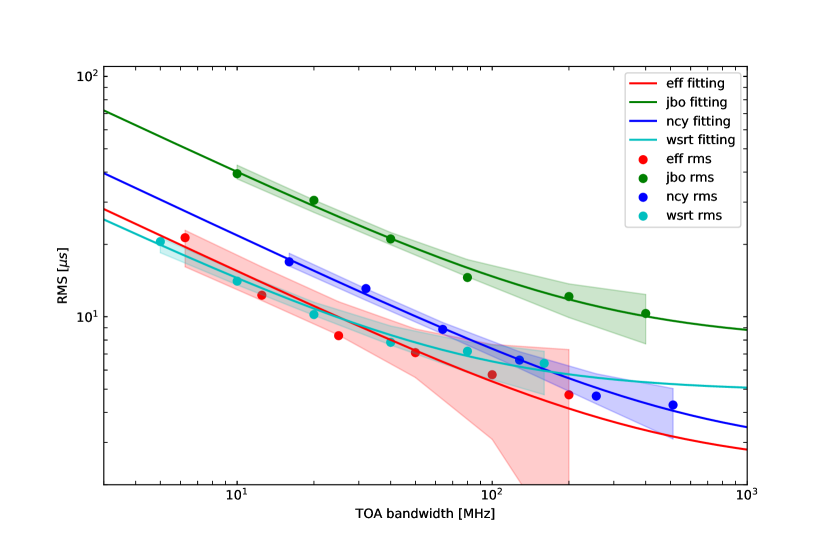
(a) ‘System limited’ noise floor estimates for PSR J0218+4232.

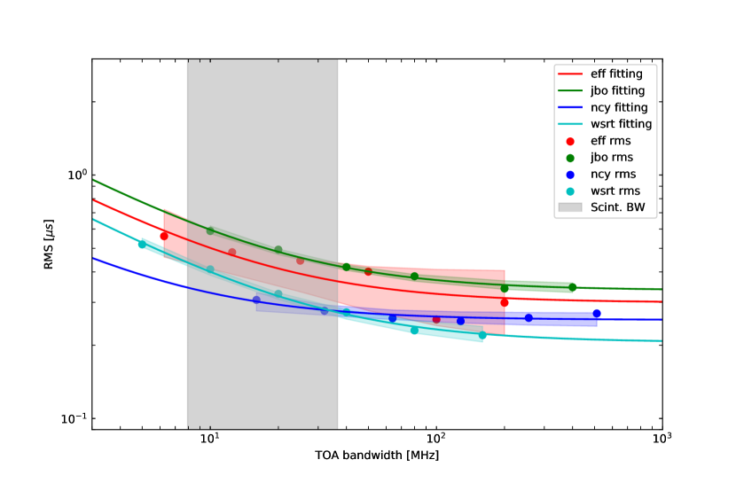
(b) ‘System limited’ noise floor estimates for PSR J1713+0747.

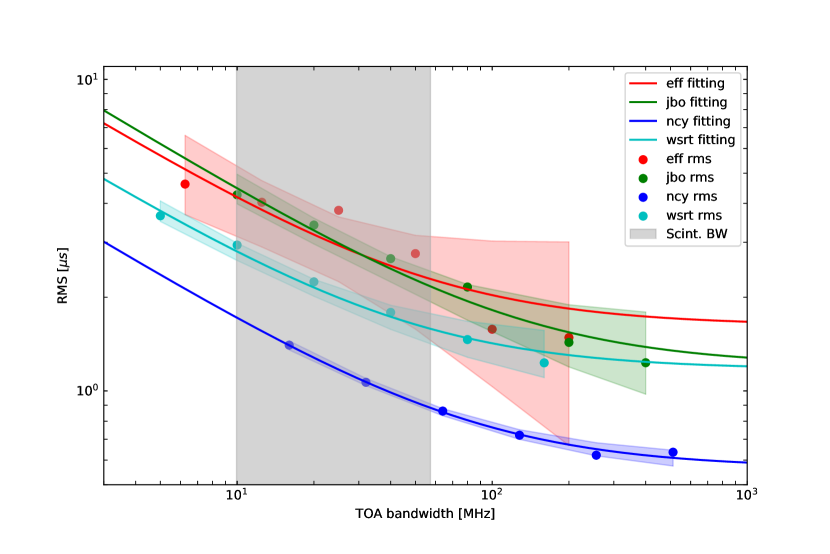
(c) ‘System limited’ noise floor estimates for PSR J2145$-$0750.

Figure 6: System limited noise floor (SLNF) estimates for the three pulsars, when using the added template with the FDM CCA to generate TOA with the available bandwidth at each telescope divided into the respective number of channels. The shaded regions along the fitted curves are the interquartile ranges for the fit, representing the error bounds on the estimated SLNF. The grey vertical bands show the expected scintillation bandwidth, estimated from the same dataset as we present here (Liu et al., 2021).

6 Conclusions

In this paper we investigated the relative merits of three common TOA determination methods and four ways to generate timing templates, by means of comparing their impact on the timing residuals and reduced $\chi^{2}$ value for data sets from four different telescopes on three different pulsars. In addition, we checked how the timing RMS reaches a plateau as TOA bandwidth is increased. This plateau or system-limited noise floor (SLNF) consists of a variety of factors, including SWIMS, instrumental noise, timing noise etc. and we have shown that it depends strongly on the telescope and pulsar in question.

With regards to the choice of the template generation scheme, we find that the single brightest observation leads to the worst timing performance. For the brighter pulsars the added, smoothed and analytic templates lead to comparable, minimum timing RMS and red. $\chi^{2}$, but for the lower S/N PSR J0218+4232 added templates can perform worse than the smoothed and analytical templates.

The analysis presented above also upholds the recommendation of Verbiest et al. (2016) that the CCA of choice for high-precision PTA work is the FDM method, although the PGS method turned out to be similarly reliable. In all pulsar, telescope and backend combinations tested above, we find that FDM and PGS TOAs lead to the most reliable TOAs and TOA uncertainties, although in the low-S/N regime both methods suffer systematic issues. Given our finding that PGS TOAs may be as reliable as FDM-based ones, particularly for bright pulsars, a re-analysis of archival data for which PGS TOAs may already be available, may well be unwarranted. In some cases, particularly when noisy templates are used, FDM does clearly outperform PGS in terms of the reliability of TOA uncertainties.

In addition, we find that GIS-derived TOAs are not suitable for high-precision timing, leading to conservative timing models and a loss of model parameter sensitivity.

Using the FDM CCA with added templates, we find that the most useful TOA bandwidth for minimising the achievable timing residual RMS is mostly dependent on the pulsar brightness and instrumental sensitivity. For the sample studied here, fully frequency-averaged TOAs seem advantageous for the relatively faint PSR J0218+4232, whereas significantly narrower bandwidths seem optimal for the brighter two pulsars in our sample.