A posteriori error estimation and adaptivity for multiple-network poroelasticity

Abstract.

The multiple-network poroelasticity (MPET) equations describe deformation and pressures in an elastic medium permeated by interacting fluid networks. In this paper, we (i) place these equations in the theoretical context of coupled elliptic-parabolic problems, (ii) use this context to derive residual-based a posteriori error estimates and indicators for fully discrete MPET solutions and (iii) evaluate the performance of these error estimators in adaptive algorithms for a set of test cases: ranging from synthetic scenarios to physiologically realistic simulations of brain mechanics.

1. Introduction

At the macroscale, the brain and other biological tissues can often be viewed as a poroelastic medium: an elastic structure permeated by one or more fluid networks. Such structures can be modeled via Biot’s equations in the case of a single fluid network [8, 9, 35] or by their generalization to the equations of multiple-network poroelasticity (MPET) which describe the case of two or more interacting fluid networks [2, 4, 5, 6, 18, 20, 36, 37, 39]. However, the computational expense associated with the numerical solution of these equations, over complex domains such as the human brain, is substantial. A natural question is therefore whether numerical error estimation and adaptivity can yield more accurate simulations of the MPET equations within a limited set of computational resources.

The quasi-static MPET equations read: given a domain $\Omega$, a finite final time $T>0$ and a set of $J$ fluid networks, find the displacement field $u:[0,T]\times\Omega\rightarrow\mathbb{R}^{d}$ and pressure fields $p_{1},p_{2}\dots p_{J}:[0,T]\times\Omega\rightarrow\mathbb{R}$ such that

$$-\operatorname{\mathrm{div}}\sigma(u)+\sum\limits_{j=1}^{J}\alpha_{j}\operatorname{\nabla}p_{j} =f,$$ (1.1a)

$$\partial_{t}\left(s_{j}p_{j}+\alpha_{j}\operatorname{\mathrm{div}}u\right)-\operatorname{\mathrm{div}}\left(\kappa_{j}\operatorname{\nabla}p_{j}\right)+T_{j} =g_{j}.$$ (1.1b)

The quantity $\sigma\left(u\right)=2\mu\varepsilon\left(u\right)+\lambda\operatorname{\mathrm{tr}}\left(\varepsilon\left(u\right)\right)\mathrm{I}$ in (1.1a) is the elastic stress tensor and involves the displacement $u$, the linearized strain tensor $\varepsilon\left(u\right)=\frac{1}{2}\left(\operatorname{\nabla}u+\operatorname{\nabla}u^{T}\right)$, the $d\times d$ identity matrix $\mathrm{I}$ and the material Lamé coefficients $\mu$ and $\lambda$. Each one of the $J$ fluid networks is associated with a Biot-Willis coefficient $\alpha_{j}$, a storage coefficient $s_{j}$, and a hydraulic conductivity $\kappa_{j}$. An interpretation of the Biot-Willis and storage coefficients, in the MPET context, appears in  [4, Section §3]. We use transfer terms $T_{j}$ in (1.1b) of the form

$$T_{j}=\sum_{i=1}^{J}T_{ji},\quad T_{ji}=\gamma_{ji}(p_{j}-p_{i}).$$ (1.2)

The coefficients $\gamma_{ji}$ regulate the interplay between network $i$ and network $j$ and $T_{j}$ is the total transfer out of network $j$ (into the other networks). The transfer term vanishes when $J=1$ and (1.1) coincides with Biot’s equations for a single fluid in a poroelastic medium. We also note that the fluid (Darcy) velocity $v_{j}$ in network $j$ is defined by

$$v_{j}=-\kappa_{j}\operatorname{\nabla}p_{j}.$$ (1.3)

Over the last decade, several authors have studied a posteriori error estimation and adaptivity related to (1.1) in the case of $J=1$; that is, for Biot’s equations of poroelasticity. Depending on the application of interest, different formulations of Biot’s equations have been used which introduce additional solution fields such as the Darcy velocity, the total pressure or the effective stress. In each case, a posteriori methods have been developed to facilitate adaptive refinement strategies. In [30], the authors consider the standard two-field formulation of Biot’s equation in two spatial dimensions, develop an a posteriori error analysis based on $H(\operatorname{\mathrm{div}})$ reconstructions of the flux and effective stress and apply the resulting estimators to construct a time-space adaptive algorithm. A posteriori estimators have also been used to provide error estimates for the popular fixed-stress iterative solution scheme applied to the two-field formulation [22]. Formulations with additional fields have also been considered for Biot’s equations. The total pressure formulation [29] is a locking-free, three-field formulation, ideal for a nearly-incompressible poroelastic material. A priori estimates, and an adaptive refinement strategy, for this formulation are constructed in [21] for quadrilateral and simplicial meshes. Residual-based a posteriori error estimates have also been advanced [24] for a lowest-order discretization of the standard Darcy-flux three-field formulation which, as shown in [31], robustly preserves convergence in the presence of vanishingly small hydraulic conductivity. Finally, a four-field formulation, with symmetric stress and a Darcy velocity, of Biot’s equations has been used to develop [1] a posteriori error estimates, and an adaptive refinement, based on post-processed pressure and displacement fields.

The a posteriori landscape for the more general MPET system (1.1) is considerably sparse. A posteriori error estimates for the two-field formulation of the Barenblatt-Biot equations (corresponding to the $J=2$ case of (1.1)) have indeed been obtained by Nordbotten et al. [27]. In general, though, there has been little work on the development of a posteriori error estimators for (1.1), for formulations with any number of fields, in the case of more than one fluid network (i.e. $J>1$). However, the recent work of [15] developed an abstract framework for a posteriori error estimators for a general class of coupled elliptic-parabolic problems.

In this manuscript, our focus is three-fold. First, we rigorously place the MPET equations in the context of coupled elliptic-parabolic problems. In particular, we consider extended spaces, bilinear forms and augmentation with a semi-inner product arising from the additional transfer terms. Second, we use this context to derive specific a posteriori error estimates and error indicators for the space-time finite element discretizations of the multiple-network poroelasticity equations in general. In biomedical applications, two-field variational formulations are often used to numerically approximate the multiple-network poroelasticity equations [36, 37], and we therefore focus on such here. Third, we formulate a physiological modelling and simulation-targeted adaptive strategy and evaluate this strategy on a series of test cases including a clinically-motivated simulation of brain mechanics.

2. Notation and preliminaries

This section provides a brief account of the notation and relevant results employed throughout the remainder of the manuscript.

2.1. Domain, boundary and meshes

It is assumed that the poroelastic domain $\Omega\subset\mathbb{R}^{d}$ with $d\in\{1,2,3\}$ is a bounded, convex domain with $\partial\Omega$ Lipschitz continuous. We consider a family of mesh discretization $\left\{\mathcal{T}_{h}\right\}_{h>0}$ of $\Omega$ into simplices; triangles when $d=2$ and tetrahedra when $d=3$. Here, $h>0$ is a characteristic mesh size such as the maximum diameter over all simplices. Furthermore, we assume that each mesh $\mathcal{T}_{h}$ in the family is quasi-uniform.

2.2. Material parameters

For simplicity, we assume that all material parameters are constant (in space), and that the following (standard) bounds are satisfied: $\mu>0$, $2\mu+\lambda>0$, $\kappa_{j}>0$, $\alpha_{j}\in(0,1]$, $s_{j}>0$ for $j=1,\dots,J$, and $\gamma_{ji}=\gamma_{ij}\geq 0$ for $i,j=1,\dots,J$ with $\gamma_{ii}=0$. The analysis can be extended to the case where the parameters, above, vary with sufficient regularity in space and time provided the above bounds hold uniformly. For each parameter, $\xi_{i}$ or $\xi_{ij}$ above, the minimum and maximum notation

$$\xi_{\max}=\max\limits_{i}\xi_{i}\text{ or }\max\limits_{ij}\xi_{ij}\quad\text{and}\quad\xi_{\min}=\min\limits_{i}\xi_{i}\text{ or }\min\limits_{ij}\xi_{ij},$$

will be used throughout the manuscript; the notational extension to the case of smoothly varying parameters, on a bounded domain with compact closure, is clear.

2.3. Norms and function spaces

Let $f$, $g$ denote real-valued functions with domain $\Omega\subset\mathbb{R}^{d}$. If there exists a generic constant $C$ with $f\leq Cg$ then we write

$$f\lesssim g.$$

The notation $\langle f,g\rangle$ signifies the usual Lebesgue inner product defined by

$$\langle f,g\rangle=\int_{\Omega}fg\,\mathrm{d}x,$$

and $||f||=\langle f,f\rangle^{1/2}$ is the corresponding norm on the Hilbert space of square-integrable functions

$$L^{2}(\Omega)=\left\{f:\Omega\rightarrow\mathbb{R}\,|\,||f||<\infty\right\}.$$

When the context is evident in praxis the domain, $\Omega$, is suppressed in the above expressions. Given $w$ a positive constant, positive scalar field, or positive-definite tensor field, the symbolics

$$\langle f,g\rangle_{w}=\langle wf,g\rangle,\quad||f||_{w}=\langle f,f\rangle_{w}^{1/2},$$

refer to a $w$-weighted inner product and norm, respectively.

The Sobolev space $H^{1}(\Omega)$, often abbreviated as simply $H^{1}$, consists of those functions $f\in L^{2}$ whereby $\partial_{x_{j}}f$ exists, in the sense of distributions, for every $j=1,2,\dots,d$ and $\partial_{x_{j}}f\in L^{2}$. The associated norm is given by the expression

$$||f||_{H^{1}}=\left(||f||^{2}+\sum\limits_{j=1}^{d}||\partial_{x_{j}}f||^{2}\right)^{1/2}.$$

The subset $H_{0}^{1}\subset H^{1}$ signifies functions with zero trace on the boundary; that is, those functions $f\in H^{1}$ such that $f(x)=0$ for almost every $x\in\partial\Omega$. In addition, given a Hilbert space $X$ with inner product $\langle\cdot,\cdot\rangle_{X}$, the notation $[X]^{d}$ refers to vectors $f=[f_{1},f_{2},\dots,f_{d}]^{T}$ whereby $f_{j}\in X$ for each $j=1,2,\dots,d$. The natural inner product on $[X]^{d}$, in which $[X]^{d}$ is also a Hilbert space, is then

$$\langle f,g\rangle=\sum\limits_{j=1}^{d}\langle f_{j},g_{j}\rangle_{X},$$

with resulting norm

$$||f||_{X^{d}}=\left(\sum\limits_{j=1}^{d}||f_{j}||_{X}^{2}\right)^{1/2}.$$

The additional decoration of the inner product, for the case of a Hilbert space $X$, will be omitted when the context is clear. For $X$ any Banach space, the notation $X^{\ast}$ denotes the dual space,and we also write $\langle x^{*},x\rangle_{X^{\prime}\times X}$ for the duality pairing. Accordingly, the operator norm on $X^{\ast}$ is denoted

$$||x^{*}||_{X^{\ast}}=\sup\limits_{||x||_{X}=1}|\langle x^{*},x\rangle_{X^{\ast}\times X}|.$$

Unlike the inner product case, the decoration of the duality pairing bracket notation will always be made explicit and never omitted.

We also recall the canonical definition [16] of some useful time-dependent spaces whose codomain is also a given Hilbert space $X$. With $X$ selected we consider a strongly measurable function $f:[0,T]\rightarrow X$. Then $f\in L^{2}(0,T;X)$ means that

$$||f||_{L^{2}(0,T;X)}=\left(\int_{0}^{T}||f(t)||_{X}^{2}\,dt\right)^{1/2}<\infty,$$

whereas $f\in L^{\infty}(0,T;X)$ implies

$$||f||_{L^{2}(0,T;X)}=\operatorname*{ess\,sup}\limits_{0\leq t\leq T}||f(t)||_{X}<\infty,$$

and $f\in C(0,T;X)$ means that

$$||f||_{C(0,T;X)}=\max\limits_{0\leq t\leq T}||f(t)||_{X}<\infty.$$

We now discuss those strongly measurable functions, $f:[0,T]\rightarrow X$, which possess weakly differentiability in time. The space $H^{1}(0,T;X)$ denotes the collection of functions, $f\in L^{2}(0,T;X)$, such that $\partial_{t}f$ exists, in the weak sense, and also resides in $L^{2}(0,T;X)$. This is similar to the usual definition of $H^{1}\left(\Omega\right)$, given above, and the norm corresponding to this space is also similar; it is given by

$$||f||_{H^{1}(0,T;X)}=\left(\int_{0}^{T}||f(t)||_{X}^{2}+||\partial_{t}f(t)||_{X}^{2}\,dt\right).$$

Likewise, $f\in C^{k}(0,T;X)$ implies that $f$ and its first $k$ weak derivatives in time, $\partial_{t}^{j}f$ for $j=1,2,\dots,k$, all reside in $C(0,T;X)$.

2.4. Mesh elements and discrete operators

For a fixed $h$, the mesh $\mathcal{T}_{h}$ is composed of simplices, denoted $T\in\mathcal{T}_{h}$, and faces (edges in 2D) $e\in\partial T$. Let $\Gamma$ denote the complete set of faces of simplices $T\in\mathcal{T}_{h}$; then $\Gamma$ can be written as the disjoint union

$$\Gamma=\Gamma_{int}\cup\Gamma_{bd},$$

where $e\in\Gamma_{int}$ if $e$ is an interior edge and $e\in\Gamma_{bd}$ if $e$ is a boundary edge.

Let $f$ be a scalar or vector valued function and suppose $e$ is an interior edge $e\in T_{+}\cap T_{-}$ where $T_{+}$ and and $T_{-}$ are two simplices with an arbitrary but fixed choice of labeling for the pairing. We denote by $n_{e}$ the outward facing normal associated to $T_{+}$. We use an explicit jump operator defined, for $e\in\Gamma_{int}$, by

$$[f]=f_{+}-f_{-}$$ (2.1)

where $f_{+}$ denotes $f$ restricted to $e\in T_{+}$ and $f_{-}$ denotes $f$ restricted to $e\in T_{-}$. For an edge $e\in\Gamma_{bd}$ we have that there exists only one $T_{+}=T\in\mathcal{T}_{h}$ such that $e\in\partial T$ and in this case we define

$$[f]=f_{+}.$$

2.5. Boundary and initial conditions

We assume homogeneous boundary conditions for the displacement and pressures; though, as in [15], these conditions can easily be generalized [32].

3. Coupled elliptic-parabolic problems as a setting for poroelasticity

To consider the a posteriori error analysis of the generalized poroelasticity equations (1.1), we follow the general framework for a posteriori error analysis for coupled elliptic-parabolic problems presented by Ern and Meunier [15]. In Section 3.1 below, we briefly overview this general framework and its application to Biot’s equations. Next, we show that (1.1) can be addressed using this general framework, also for the case where $J>1$ under appropriate assumptions on the transfer terms $T_{m\rightarrow n}$, in Section 3.2. Based on the general framework, Ern and Meunier derive and analyze several a posteriori error estimators. These estimators, and their corresponding extensions to the generalized poroelasticity equations, will be discussed in Section 5.

3.1. The coupled elliptic-parabolic problem framework

The setting introduced by Ern and Meunier [15] for coupled elliptic-parabolic problems provides a natural setting also for generalized poroelasticity. The general coupled elliptic-parabolic problem reads as: find $(u,p)\in H^{1}(0,T;V_{a})\times H^{1}(0,T;V_{d})$ that satisfy (for almost every $t\in[0,T]$):

$$a(u,v)-b(v,p) =\langle f,v\rangle_{V_{a}^{\ast}\times V_{a}},\quad\forall\,v\in V_{a},$$ (3.1a)

$$c(\partial_{t}p,q)+b(\partial_{t}u,q)+d(p,q) =\langle g,q\rangle_{V_{d}^{\ast}\times V_{d}}.\quad\forall\,q\in V_{d}.$$ (3.1b)

The data, $f$ and $g$ in (1.1), are general and assumed to satisfy $f\in H^{1}(0,T;V_{a}^{*})$ and $g\in H^{1}(0,T;V_{d}^{*})$. The initial pressure is assumed to satisfy $p(0)\in V_{d}$. Moreover, it is assumed that

1. $V_{a}$ and $V_{d}$ are Hilbert spaces.

2. $a:V_{a}\times V_{a}\rightarrow\mathbb{R}$ and $d:V_{d}\times V_{d}\rightarrow\mathbb{R}$ are symmetric, coercive, and continuous bilinear forms, thus inducing associated inner-products and norms (denoted by $\|\cdot\|_{a}$ and $\|\cdot\|_{d}$) on their respective spaces.

3. There exist Hilbert spaces $L_{a}$ and $L_{d}$ with $V_{a}\subset L_{a}$ and $V_{d}\subset L_{d}$, where the inclusion is dense and such that $||f||_{L_{a}}\lesssim||f||_{a}$ for $f\in V_{a}$, and $||g||_{L_{d}}\lesssim||g||_{d}$ for $g\in V_{d}$.

4. $c:L_{d}\times L_{d}\rightarrow\mathbb{R}$ is symmetric, coercive and continuous; thereby defining an equivalent norm $\|\cdot\|_{c}$, on $L_{d}$.

5. There exists a continuous bilinear form $b:V_{a}\times L_{d}\rightarrow\mathbb{R}$ such that $|b(f,g)|\lesssim\|f\|_{a}\|g\|_{c}$ for $f\in V_{a}$ and $g\in L_{d}$.

Example 3.1.

Biot’s equations of poroelasticity (i.e. (1.1) for $J=1$ fluid networks) fit the coupled elliptic-parabolic framework with

$$V_{a}=\left[H_{0}^{1}\right]^{d},\quad L_{a}=\left[L^{2}\right]^{d},\quad V_{d}=H_{0}^{1},\quad L_{d}=L^{2}.$$

and

$$a(u,v) =\langle\sigma(u),\varepsilon(v)\rangle,$$

$$b(u,p) =\langle\alpha_{1}p,\operatorname{\mathrm{div}}u\rangle,\quad c(p,q)=\langle c_{1}p,q\rangle,\quad d(p,q)=\langle\kappa_{1}\operatorname{\nabla}p,\operatorname{\nabla}q\rangle,$$

with the standard (vector) $H^{1}_{0}$-inner product and norm on $V_{a}$ and $V_{d}$, and $L^{2}$-inner product and norm on $L_{a}$ and $L_{d}$. It is readily verifiable that the general conditions described above are satisfied under these choices of spaces, norms, inner products and forms [15]. The existence and uniqueness of solutions to Biot’s equations of poroelasticity ($J=1$ in (1.1) and (3.1) with the above bilinear forms) is now a classical result [32].

3.2. Generalized poroelasticity as a coupled elliptic-parabolic problem

In this section, we derive a variational formulation of the generalized poroelasticity equations (1.1) for the case of several fluid networks (i.e. $J\geq 1$) and show how this formulation fits the general framework presented above. The extension from Biot’s equations to generalized poroelasticity is natural in the sense it coincides with the original application of the general framework to Biot’s equations when $J=1$. Suppose that the total number of networks $J$ is arbitrary but fixed. We define the spaces

$$V_{a}=\left[H_{0}^{1}\right]^{d},\quad L_{a}=\left[L^{2}\right]^{d},\quad V_{d}=\left[H_{0}^{1}\right]^{J},\quad L_{d}=\left[L^{2}\right]^{J}.$$ (3.2)

We consider data such that $f\in H^{1}(0,T;L_{a})$ and $(g_{1},g_{2},\dots,g_{J})\in H^{1}(0,T;L_{d})$ with given initial network pressures determined by $p(0)\in V_{d}$. A standard multiplication, integration and integration by parts yield the following variational formulation of (1.1): find $u\in H^{1}(0,T;V_{a})$ and $p=(p_{1},\dots,p_{J})\in H^{1}(0,T;V_{d})$ such that for a.e. $t\in(0,T]$:

$$\langle\sigma(u),\varepsilon(v)\rangle{-}\textstyle\sum_{j=1}^{J}\langle\alpha_{j}p_{j},\operatorname{\mathrm{div}}v\rangle =\langle f,v\rangle,$$ (3.3a)

$$\textstyle\sum_{j=1}^{J}\langle\partial_{t}s_{j}p_{j},q_{j}\rangle+\langle\partial_{t}\alpha_{j}\operatorname{\mathrm{div}}u,q_{j}\rangle+\langle\kappa_{j}\operatorname{\nabla}p_{j},\operatorname{\nabla}q_{j}\rangle+\langle T_{j},q_{j}\rangle =\textstyle\sum_{j=1}^{J}\langle g_{j},q_{j}\rangle.$$ (3.3b)

for $v\in V_{a}$, $q=(q_{1},\dots,q_{J})\in V_{d}$. As noted in [15], (3.3a) holds up to time $t=0$ so that $u_{0}$ is determined by the initial data $p(0)$ and initial right-hand side $f(0)$. By labeling the forms

$$a(u,v) =\langle\sigma(u),\varepsilon(v)\rangle,$$ (3.4a)

$$b(u,p) =\textstyle\sum_{j=1}^{J}\langle\alpha_{j}p_{j},\operatorname{\mathrm{div}}u\rangle,$$ (3.4b)

$$c(p,q) =\textstyle\sum_{j=1}^{J}\langle s_{j}p_{j},q_{j}\rangle,$$ (3.4c)

$$d(p,q) =\textstyle\sum_{j=1}^{J}\langle\kappa_{j}\operatorname{\nabla}p_{j},\operatorname{\nabla}q_{j}\rangle+\langle T_{j},q_{j}\rangle,$$ (3.4d)

we observe that the weak formulation (3.3) of (1.1) takes the form (3.1) where $T_{j}$, in (3.4d), is given by (1.2).

Remark 3.1.

Existence and uniqueness of solutions to (3.3), with forms (3.4), for the case of $J=2$ (Barenblatt-Biot) have been established [33]. However, to our knowledge, a rigorous treatment of existence and uniqueness of solutions to (1.1), (3.3) for $J>2$ remains an open problem despite their otherwise successful use in applications [18, 19, 36, 37].

We now show that the associated assumptions on these forms and spaces hold, beginning with properties of the form $d$ in Lemma 3.2 below.

Lemma 3.2.

The form $d$ given by (3.4d) defines an inner product over $[H^{1}_{0}(\Omega)]^{J}$ with associated norm

$$\|q\|_{d}^{2}=d(q,q)=\textstyle\sum_{j=1}^{J}\|\operatorname{\nabla}q_{j}\|_{\kappa_{j}}^{2}+|q|_{T}^{2},\quad\forall\,q\in V_{d},$$ (3.5)

where $|\cdot|_{T}$ is defined by (3.7), which is such that

$$\|q\|_{d}\lesssim\|q\|_{H^{1}_{0}},\quad\forall\,q\in[H^{1}_{0}]^{J},$$ (3.6)

with inequality constant depending on $J$, $\kappa_{\max}$, $\gamma_{\max}$ and $\Omega$.

Proof.

By definition (1.2) and the assumption of symmetric transfer $\gamma_{ji}=\gamma_{ij}\geq 0$, we have

$$\textstyle\sum_{j=1}^{J}\langle T_{j},q_{j}\rangle=\textstyle\sum_{j=1}^{J}\textstyle\sum_{i=1}^{J}\langle\gamma_{ji}(p_{j}-p_{i}),q_{j}\rangle=\frac{1}{2}\textstyle\sum_{j=1}^{J}\textstyle\sum_{i=1}^{J}\langle\gamma_{ji}(p_{j}-p_{i}),(q_{j}-q_{i})\rangle.$$ (3.7)

Given $p$, $q\in V_{d}$, the bilinear form defined by (3.7), that is

$$\langle p,q\rangle_{T}=\textstyle\sum_{j=1}^{J}\langle T_{j},q_{j}\rangle,$$

is clearly symmetric and satisfies the requirements of a (real) semi-inner product on $L_{d}\times L_{d}$ in the sense of [11]. It follows that

$$|q|_{T}\equiv\langle q,q\rangle_{T}^{1/2}=\left(\frac{1}{2}\textstyle\sum_{j=1}^{J}\textstyle\sum_{i=1}^{J}\langle\gamma_{ji}(q_{j}-q_{i}),(q_{j}-q_{i})\rangle\right)^{1/2}$$ (3.8)

defines a semi-norm on $L_{d}\times L_{d}$ and that the corresponding Cauchy-Schwarz inequality holds. Using the triangle inequality, the definition (3.7), the bounds for $\gamma_{ji}$ and the Poincaré inequality, we have that

$$|q|_{T}\lesssim\|q\|_{[L^{2}]^{J}}\lesssim\|q\|_{[H^{1}_{0}]^{J}}$$ (3.9)

with constant depending on $\gamma_{\max}$, $J$, and the domain via the Poincaré constant. Under the assumption that $\kappa_{\min}>0$, we observe that as a result $d$ defines an inner product and norm on $[H^{1}_{0}]^{J}\times[H^{1}_{0}]^{J}$. Similarly, (3.6) holds with with constant depending on $\kappa_{\max}$ in addition to $\gamma_{\max}$, $J$, and the domain $\Omega$. ∎

Lemma 3.2 will be used in the subsequent sections. We next show that the choices of spaces (3.2) and forms (3.4) satisfy the abstract assumptions of the framework as overviewed in Section 3.1, and summarize this result in Lemma 3.3.

Lemma 3.3.

The problem (3.3), arising from the equations of generalized poroelasticity (1.1) with material parameters as in Section 2.2, posed on the spaces (3.2) with bilinear forms defined via (3.2) is a coupled elliptic-parabolic problem and satisfy the assumptions set forth in [15].

Proof.

We consider each assumption in order. These are standard results, but explicitly included here for the sake of future reference.

1. $V_{a}$ and $V_{d}$ defined by (3.2) are clearly Hilbert spaces with natural Sobolev norms $\|\cdot\|_{H^{1}_{0}}$.

2. $a$ is symmetric, coercive on $V_{a}$ by Korn’s inequality and the lower bounds on $\mu$, $2\mu+d\lambda$, and continuous (with continuity constant depending on $\mu_{\max}$ and $\lambda_{\max}$). $d$ is clearly symmetric by the transfer symmetry assumption and (3.7), coercive by $|\cdot|_{T}\geq e0$ and the assumption that $\kappa_{\min}>0$:

   $$d(q,q)\geq\textstyle\sum_{j=1}^{J}\langle\operatorname{\nabla}q_{j},\operatorname{\nabla}q_{j}\rangle_{\kappa_{j}}\geq\kappa_{\min}\textstyle\sum_{j=1}^{J}\|q_{j}\|_{H_{0}^{1}}^{2},$$

   and continuous by Lemma 3.2.

3. The embedding of $(V_{a},\|\cdot\|_{a})$ into $L_{a}$ follows from Poincare’s inequality and the coercivity of $a$ over $V_{a}$ and similarly for $V_{d}\hookrightarrow L_{d}$.

4. $c$ is symmetric by definition, continuous over $L_{d}$ with continuity constant depending on $c_{\max}$, and coercive with coercivity constant depending on $c_{\min}>0$.

5. The form $b$ given by (3.4b) is clearly bilinear and continuous on $V_{a}\times L_{d}$ as

   $$|b(u,p)| =|\sum\limits_{j=1}^{J}\langle p_{j},\operatorname{\mathrm{div}}u\rangle_{\alpha_{j}}|\lesssim||u||_{H^{1}}\left(\sum\limits_{j=1}^{J}||p_{j}||^{2}\right)^{\frac{1}{2}}=||u||_{H^{1}}||p||_{[L^{2}]^{J}}\lesssim\|u\|_{a}\|p\|_{c}$$

   by applying Cauchy-Schwarz and Hölder’s inequality, with constant depending on $\alpha_{\min}>0$ and the coercivity constants of $a$ and $c$. ∎

In light of Lemma 3.3, the generalized poroelasticity system (3.3) is of coupled elliptic-parabolic type and takes the form of (3.1) with bilinear forms defined by (3.4).

Corollary 3.4.

The following energy estimates hold for almost every $t\in[0,T]$

$$||u(t)||_{a}^{2}+ \textstyle\sum\limits_{j=1}^{J}s_{j}||p_{j}(t)||^{2}+\textstyle\sum\limits_{j=1}^{J}\int_{0}^{t}\kappa_{j}||\operatorname{\nabla}p(s)||^{2}\,\text{d}s+\textstyle\sum\limits_{i=1}^{J}\textstyle\sum\limits_{j=1}^{J}\int_{0}^{t}\gamma_{ij}||p_{j}(s)-p_{i}(s)||^{2}\,\text{d}s$$

$$\lesssim\left(\sup\limits_{s\in[0,T]}||f(s)||+\int_{0}^{T}||\partial_{t}f(s)||\,\text{d}s\right)^{2}+\int_{0}^{T}||g(s)||^{2}\,\text{d}s+||u_{0}||_{a}^{2}+\textstyle\sum\limits_{j=1}^{J}s_{j}||p_{0}||^{2}$$

Proof.

The proof follows directly from Lemma 3.3, the corresponding energy estimates for coupled elliptic-parabolic systems [15, Prop. 2.1] and the definition of the norms arising from the forms (3.4). Moreover, the proportionality constant in the estimates is independent of all material parameters and the number of networks. ∎

Remark 3.2.

The elliptic-parabolic MPET energy estimates, of Corollary 3.4, are similar to those of the total pressure formulation [23, Theorem 3.3] when the second Lamé coefficient, $\lambda$, is held constant in the latter. The primary difference is that [23] separates the estimates of $u$ from that of the solid pressure, $\lambda\operatorname{\mathrm{div}}u$, by including the latter term into a ‘total pressure’ variable. This allows for $||u||_{1}$ to be estimated directly, in [23], regardless of the value of $\lambda$ used in the definition of $||u||_{a}$.

Remark 3.3.

The conditions of Section 3.1, i.e. conditions (2)-(5), can place restrictions on the generalized poroelastic setting. As an example, the assumption of a vanishing storage coefficient has appeared in the literature as a modeling simplification [25, 40]. However, the coercivity requirement of condition (4) precludes the use of a vanishing specific storage coefficient, $s_{j}$ in (3.4c), for any network number $j=1,2,\dots,J$. Care should be taken to ensure that any modeling simplifications produce forms that satisfy the conditions of Section 3.1 in order for the results of Corollary 3.4 and Section 4 to hold.

4. Discretization and a priori error estimates

4.1. An Euler-Galerkin discrete scheme

We now turn to an Euler-Galerkin discretization of (1.1) in the context of such discretizations of coupled elliptic-parabolic problems in general [15]. We employ an implicit Euler discretization in time and conforming finite elements in space.

We consider a family of simplicial meshes $\left\{\mathcal{T}_{h}\right\}_{h>0}$ with $h$ a characteristic mesh size such as the maximal element diameter

$$h=\max\left\{h_{K}=\textrm{diam}(K)\,|\,K\in\mathcal{K}_{h}\right\}.$$

Furthermore, let $\{V_{a,h}\}_{h}$ and $\{V_{d,h}\}_{h}$ denote two families of finite dimensional subspaces of $V_{a}$ and $V_{d}$, as in (3.2), respectively, defined relative to $\{\mathcal{T}_{h}\}_{h}$. For a final time $T>0$ we let $0=t_{0}<t_{1}<\dots<t_{N}=T$ denote a sequence of discrete times and set $\tau_{n}=t_{n}-t_{n-1}$. For functions and fields, we use the superscript $n$ to refer values at time point $t_{n}$. We also utilize the discrete time differential notation $\delta_{t}$ where

$$\delta_{t}u_{h}^{n}=\tau_{n}^{-1}\left(u_{h}^{n}-u_{h}^{n-1}\right).$$ (4.1)

With this notation, the discrete problem is to seek $u_{h}^{n}\in V_{a,h}$ and $p_{h}^{n}=(p_{1,h}^{n},p_{2,h}^{n},\dots,p_{J,h}^{n})\in V_{d,h}$ such that for all time steps $t_{n}$ with $n\in\left\{1,2,\dots,N\right\}$:

$$a(u_{h}^{n},v_{h})-b(v_{h},p_{h}^{n}) =\langle f_{h}^{n},v_{h}\rangle \quad\forall\,v_{h}\in V_{a,h},$$ (4.2a)

$$c(\delta_{t}p_{h}^{n},q_{h})+b(\delta_{t}u_{h}^{n},q_{h})+d(p_{h}^{n},q_{h}) =\langle g_{h}^{n},q_{h}\rangle \quad\forall\,q_{h}\in V_{d,h},$$ (4.2b)

where the spaces and forms are defined by (3.2) and (3.4). The right-hand sides, above, express the inner product of the discrete approximations $f_{h}^{n}\in L_{a,h}$, to $f$ and $g_{h}^{n}\in L_{d,h}$, to $g$, at time $t_{n}$. By Lemma 3.3 and [15, Lemma 2.1], the discrete system (4.2) is well-posed.

4.2. A priori error estimates

Now, let $V_{a,h}$ and $V_{d,h}$ be spatial discretizations arising from continuous Lagrange elements of order $k_{a}$ and $k_{d}$, respectively, where $k_{d}=k_{a}-1$; this relation on relative degree results directly from the framework hypotheses [15, Section 2]. Let $\mathcal{P}_{k}(T)$ denote polynomials of order $k$ on a simplex $T\in\mathcal{T}_{h}$. We consider the continuous Lagrange polynomials of order $k_{a}$ and $k_{a-1}$ defined by

$$V_{a,h} =\left\{v_{h}\in C^{0}(\bar{\Omega})\,|\,v_{h|T}\in\mathcal{P}_{k_{a}}(T)\text{ for every }T\in\mathcal{T}_{h}\right\},$$ (4.3)

$$V_{d,h} =\left[\left\{q_{h}\in C^{0}(\bar{\Omega})\,|\,q_{h|T}\in\mathcal{P}_{k_{a}-1}(T)\text{ for every }T\in\mathcal{T}_{h}\right\}\right]^{J}$$ (4.4)

as the discrete spaces for the displacement and network pressures, respectively. When $J=1$ this choice coincides with the previous [15] discretization considered for Biot’s equations.

The general framework stipulates that three hypotheses [15, Section 2.5], restated here for completeness, should be satisfied for the discretization.

Hypothesis 4.1.

There exists positive real numbers, denoted $s_{a}$ and $s_{d}$, and subspaces, $W_{a}\subset V_{a}$ and $W_{d}\subset V_{d}$ equipped with norms $||\cdot||_{W_{a}}$ and $||\cdot||_{W_{d}}$, such that the following estimates hold independently of $h$

$$\forall v\in W_{a},\quad \inf_{v_{h}\in V_{a,h}}||v-v_{h}||_{a}\lesssim h^{s_{a}}||v||_{W_{a}},$$ (4.5)

$$\forall q\in W_{d},\quad \inf_{q_{h}\in V_{d,h}}||q-q_{h}||_{d}\lesssim h^{s_{d}}||q||_{W_{d}}.$$ (4.6)

Hypothesis 4.2.

There exists a real number $\delta$ such that for every $r\in L_{d}$, the unique solution $\phi\in V_{d}$ for the dual problem

$$d(q,r)=c(r,q)\quad\forall q\in V_{d},$$

is such that there exists $\phi_{h}\in V_{d,h}$ satisfying

$$||\phi-\phi_{h}||_{d}\lesssim h^{\delta}||r||_{c}.$$

Hypothesis 4.3.

$s_{a}$ = $s_{d}+\delta$

We now state the primary result of this section.

Lemma 4.4.

The discrete two-field variational formulation of the MPET equations (4.2) with the choice of discrete spaces $V_{a,h}$ (4.3) and $V_{d,h}$ (4.4) satisfy the elliptic-parabolic framework hypotheses 4.1–4.3, above.

Proof.

Choose $s_{a}=k_{a}$ and $s_{d}=k_{a-1}$. Then the conditions of Hypothesis 4.1 follow, as in [15], from choosing $W_{a}=\left[H_{0}^{1}\cap H^{k_{a+1}}(\mathcal{T}_{h})\right]^{3}$ and $W_{d}=\left[H_{0}^{1}\cap H^{k_{a}}(\mathcal{T}_{h})\right]^{J}$ where $H^{k}(\mathcal{T}_{h})$ denotes the broken Sobolev space of order $k$ on the mesh $\mathcal{T}_{h}$. The estimate (4.5) follows, without extension, directly from classical results in approximation theory [14]; precisely as discussed in [15]. Similarly, the estimate (4.6) follows from the properties of $d$, standard interpolation estimates [14], and the product structure of $V_{d}$ and $V_{d,h}$.

For hypothesis 4.2, we use the elliptic regularity, c.f. standard well posedness and interior regularity arguments in [16, Chp. 6], of the solution to the coupled linear diffusion-reaction equation of finding $\phi\in V_{d}$ such that

$$A\phi+\Gamma\phi=R\,\quad\text{for }R\in L_{d},$$

where $A$ is the $J\times J$ diagonal Laplacian matrix

$$\left(\begin{array}[]{cccc}-\Delta&0&\dots&0\\ 0&-\Delta&\dots&0\\ \vdots&\ddots&\ddots&\vdots\\ 0&0&0&-\Delta\end{array}\right),$$ (4.7)

and $\Gamma$ is a matrix composed of the transfer coefficients $\gamma_{ij}$: $\Gamma_{ii}=\sum_{j}\gamma_{ji}$, and $\Gamma_{ij}=-\gamma_{ij}$ for $j\not=i$. It follows from Lemma 3.2, and $\Gamma$ symmetric and positive-semi definite, that the solution $\phi\in V_{d}$ to the dual problem

$$d(w,\phi)=c(R,w)=\langle R,w\rangle_{L_{d}^{\prime},V_{d}},\quad\text{for all }w\in V_{d},$$ (4.8)

lies in $\left[H^{2}\right]^{J}$ with $||\phi||_{H^{2}}\lesssim||R||_{L_{d}}=||R||_{c}$. Using this and standard interpolation results we have $\phi_{h}\in V_{d,h}$ with

$$||\phi-\phi_{h}||_{d}\lesssim h^{\delta}||R||_{c}=h^{\delta}||R||_{L_{d}},$$

where $\delta=1$; exactly as in [15]. Finally, with $\delta=1$ and the choices $s_{a}=k_{a}$ and $s_{d}=k_{a}-1$, hypothesis 4.3 also holds. ∎

A priori estimates for the Euler-Galerkin discretization (4.2) of the generalized poroelasticity equations (1.1) then follow directly from [15, Theorem 3.1]. These estimates will be used in the a posteriori analysis and are restated from [15], subject to the extended spaces and forms of (3.2) and (3.4).

Corollary 4.5 (A priori estimates for generalized poroelasticity).

Let $I_{n}=[t_{n-1},t_{n}]$ denote the $n^{th}$ time sub-interval of $[0,T]$ for $n=1,2,\dots N$ of length $\tau_{n}=t_{n}-t_{n-1}$. Suppose the exact solution $(u,p)$ to (3.3) satisfies $u\in C^{1}(0,T;W_{a})\cap C^{2}(0,T;V_{a})$ and $p\in C^{1}(0,T;W_{d})\cap C^{2}(0,T;L_{d})$, where $W_{a}$ and $W_{d}$ are given above with $V_{a}$ and $L_{d}$ as in (3.2). It is also assumed that the initial data satisfies

$$||u_{0}-u_{0,h}||_{a}\lesssim h^{k_{a}}||u_{0}||_{W_{a}}\quad\text{and}\quad||p_{0}-p_{0,h}||_{c}\lesssim h^{k_{a}}||p_{0}||_{W_{d}}.$$

Define

$$C_{1}^{n}(u,p) =||\partial_{t}p(s)||_{L^{\infty}(I_{n};W_{d})}^{2}+||\partial_{t}u(s)||_{L^{\infty}(I_{n};W_{a})}^{2},$$

$$C_{2}^{n}(u,p) =||\partial_{tt}^{2}p(s)||_{L^{\infty}(I_{n};L_{d})}^{2}+||\partial_{tt}^{2}u(s)||_{L^{\infty}(I_{n};V_{a})}^{2},$$

$$C^{n}(f,g) =||f^{n}-f_{h}^{n}||_{a}^{2}+\tau_{n}||g^{n}-g_{h}^{n}||_{d}^{2},$$

$$C(u_{0},p_{0}) =||u_{0}||_{W_{a}}^{2}+||p_{0}||_{W_{d}}^{2}.$$

Setting, for simplicity, $s=k_{a}$ then $s=k_{d}+1$, by the selection of the discrete spaces, and we have that for each $n\in\left\{1,2,\dots,N\right\}$

$$\begin{split}||u^{n}-u_{h}^{n}||_{a}^{2}+||p^{n}-p_{h}^{n}||_{c}^{2}\lesssim h^{2s}C(u_{0},p_{0})+\sum\limits_{m=1}^{n}C^{m}(f,g)+\sum\limits_{m=1}^{n}\tau_{m}h^{2s}C_{1}^{m}(u,p)\\ \quad\quad+\sum\limits_{m=1}^{n}\tau_{m}^{3}C_{2}^{m}(u,p)+h^{2s}\left(||u^{n}||_{W_{a}}^{2}+||p^{n}||_{W_{d}}^{2}\right),\end{split}$$ (4.9)

and

$$\begin{split}\sum\limits_{m=1}^{n}\tau_{m}||p^{m}-p_{h}^{m}||_{d}^{2}\lesssim h^{2s}C(u_{0},p_{0})+\sum\limits_{m=1}^{n}C^{m}(f,g)+\sum\limits_{m=1}^{n}\tau_{m}h^{2s}C_{1}^{m}(u,p)\\ \quad\quad+\sum\limits_{m=1}^{n}\tau_{m}^{3}C_{2}^{m}(u,p)+\sum\limits_{m=1}^{n}\tau_{m}h^{2s-1}||p^{m}||_{W_{d}}^{2}.\end{split}$$ (4.10)

5. A posteriori error estimation for generalized poroelasticity

We now turn to discuss the implications to a posteriori error estimates for generalized poroelasticity as viewed through the lens of the coupled elliptic-parabolic problem framework. Our focus is to derive, apply and evaluate residual-based error estimators and indicators in the context of generalized poroelasticity. We will therefore present an explicit account of abstractly defined quantities presented in [15, Sec. 4.1], including e.g. the Galerkin residuals, applied in our context.

5.1. Time interpolation

We now recall additional notation for time interpolation (from [15, Sec. 4.1]), and rewrite (4.2). Let $u_{h\tau}$ denote the continuous and piecewise linear function in time, $u_{h\tau}\in H^{1}(0,T;V_{a,h})$ such that $u_{h\tau}(t_{n})=u_{h}^{n}$. Similarly $(p_{1h\tau},p_{2,h\tau},\dots,p_{J,h\tau})=p_{h\tau}$ is defined by $p_{h\tau}(t_{n})=p_{h}^{n}$ and extended linearly in time. As a result, $\partial_{t}u_{h\tau}$, $\partial_{t}p_{h\tau}$ are defined for almost every $t\in(0,T)$. Define the corresponding continuous, piecewise linear in time variants of the data, $f_{h\tau}$ and $g_{h\tau}$, by the same approach; i.e. $f_{h\tau}(t_{n})=f_{h}^{n}$ and $g_{h\tau}(t_{n})=g_{h}^{n}$.

Before rephrasing (4.2) using the time-interpolated variables we define piecewise constant functions in time for the pressure and right-hand side data. These are defined as $\pi^{0}p_{h\tau}=p_{h}^{n}$ and $\pi^{0}g_{h\tau}=g_{h}^{n}$ on $I_{n}=(t_{n-1},t_{n})$. Using the above notation, the discrete scheme for almost every $t\in(0,T)$ becomes

$$a(u_{h\tau},v_{h})-b(v_{h},p_{h\tau}) =\langle f_{h\tau},v_{h}\rangle,\quad\quad\forall v\in V_{a,h},$$ (5.1a)

$$c(\partial_{t}p_{h\tau},q_{h})+b(\partial_{t}u_{h\tau},q_{h})+d(\pi^{0}p_{h\tau},q_{h}) =\langle\pi^{0}g_{h\tau},q_{h}\rangle,\quad\forall q_{h}\in{\color[rgb]{0,0,0}V_{d,h}}.$$ (5.1b)

Remark 5.1.

Using the linear time interpolations defined above, such as $u_{h\tau}$ or $p_{h\tau}$, we have the following identity

$$\partial_{t}u_{h\tau}=\delta u_{h}^{n}\quad\text{for all }t\in I_{n}=(t_{n-1},t_{n}),$$

so that the left-hand sides of and (4.2b) and (5.1b) are identical. However, as noted in [15], the interpolants of the data, $f_{h\tau}$ and $g_{h\tau}$, are continuous and facilitate the definition of the continuous-time residuals (5.2) and (5.3).

5.2. Galerkin residuals

The Galerkin residuals [15, Section 4.1] are functions of time whose co-domain lies in the dual of either $V_{a}$ or $V_{d}$. More specifically, the residuals are continuous, piecewise-affine functions $\mathcal{G}_{a}:[0,T]\rightarrow V_{a}^{*}$ and $\mathcal{G}_{d}:[0,T]\rightarrow V_{d}^{*}$. In our context, of generalized poroelasticity, the Galerkin residual $\mathcal{G}_{a}$ is, given any $v\in V_{a}$, defined by the relation

$$\langle\mathcal{G}_{a},v\rangle\equiv\langle f_{h\tau},v\rangle-a(u_{h\tau},v)+b(v,p_{h\tau})=\langle f_{h\tau},v\rangle-a(u_{h\tau},v)+\sum\limits_{j=1}^{J}\langle p_{j,h\tau},\operatorname{\mathrm{div}}v\rangle_{\alpha_{j}}.$$ (5.2)

Similarly, $\mathcal{G}_{d}$ is, given any $q=(q_{1},q_{2},\dots,q_{J})\in V_{d}$, defined by the relation

$$\begin{split}\langle\mathcal{G}_{d},q\rangle&\equiv\langle\pi^{0}g,q\rangle-c(\partial_{t}p_{h\tau},q)-b(\partial_{t}u_{h\tau},q)-d(\pi^{0}p_{h\tau},q)\\ &=\sum\limits_{j=1}^{J}\langle\pi^{0}g_{j,h\tau},q_{j}\rangle-\sum\limits_{j=1}^{J}\langle s_{j}\partial_{t}p_{j,h\tau},q_{j}\rangle-\sum\limits_{j=1}^{J}\langle\alpha_{j}\partial_{t}\operatorname{\mathrm{div}}u_{h\tau},q_{j}\rangle\\ &\qquad-\sum\limits_{j=1}^{J}\langle\kappa_{j}\operatorname{\nabla}p_{j},\operatorname{\nabla}q_{j}\rangle+\frac{1}{2}\sum\limits_{j=1}^{J}\sum\limits_{i=1}^{J}\langle\gamma_{ij}(p_{j,h\tau}-p_{i,h\tau}),(q_{j}-q_{i})\rangle,\end{split}$$ (5.3)

Again, we note that (5.2) and (5.3) generalize the corresponding [15, Sec. 4.1] residuals for the case of single-network poroelasticity studied therein.

5.3. Data, space and time estimators

The general coupled elliptic-parabolic problem framework gives a posteriori error estimates, and in particular so-called data, space and time estimators for the discrete solutions. In our context of generalized poroelasticity, these can be expressed explicitly as follows. We have terms for the data $f$ and $g$ given by

$$\mathcal{E}(f,g)=||g-\pi^{0}g_{h\tau}||_{L^{2}(0,T;V_{a}^{\ast})}^{2}+\left(||f-f_{h\tau}||_{L^{\infty}(0,T;V_{a}^{\ast})}+||\partial_{t}(f-f_{h\tau})||_{L^{1}(0,T;V_{a}^{\ast})}\right)^{2},$$

and the framework data, space and time estimators are defined, respectively, as

$$\mathcal{E}_{\text{data}} =||u_{0}-u_{0h}||_{a}^{2}+||p_{0}-p_{0h}||_{c}^{2}+\mathcal{E}(f,g),$$ (5.4)

$$\mathcal{E}_{\text{space}} =||\mathcal{G}_{d}||_{L^{2}(0,T;V_{d}^{\ast})}^{2}+\left(||\mathcal{G}_{a}||_{L^{\infty}(0,T;V_{a}^{\ast})}+||\partial_{t}\mathcal{G}_{a}||_{L^{1}(0,T;V_{a}^{\ast})}\right)^{2},$$ (5.5)

$${\color[rgb]{0,0,0}\mathcal{E}_{\text{time}}} ={\color[rgb]{0,0,0}||p_{h\tau}-\pi^{0}p_{h\tau}||_{L^{2}(0,T;V_{d})}^{2}},$$ (5.6)

where we recall that the norms are now defined according to the extended generalized poroelasticity spaces (3.2) and forms (3.4). The following a posteriori error estimate for the general MPET equations holds:

Proposition 5.1.

For every time $t_{n}$, with $n\in\left\{1,2,\dots,N\right\}$, the following inequality holds

$$||u-u_{h\tau}||_{L^{\infty}(0,t_{n};V_{a})}^{2}+||p-p_{h\tau}||_{L^{\infty}(0,t_{n};L_{d})}^{2}+||p-p_{h\tau}||_{L^{2}(0,t_{n};V_{d})}^{2}$$ (5.7)

$$\qquad+||p-\pi^{0}p_{h\tau}||_{L^{2}(0,t_{n};V_{d})}^{2}\lesssim\mathcal{E}_{\text{data}}+\mathcal{E}_{\text{space}}+\mathcal{E}_{\text{time}}$$ (5.8)

Proof.

The proof follows from [15, Thm. 4.1] and the arguments of Section 3.2. ∎

Remark 5.2.

Note [15, eqn. (4.10)] that (5.6) is equivalent to

$$\mathcal{E}_{\text{time}}=\frac{1}{3}\sum\limits_{m=1}^{N}\tau_{m}||p_{h}^{m}-p_{h}^{m-1}||_{d}^{2},\quad m\in\left\{1,2,\dots,N\right\}.$$

The above expression will be used in Section 5.6 and follows, via the definition of $p_{h\tau}$ and $\pi^{0}$, from the calculation

$$||p_{h\tau}-\pi^{0}p_{h\tau}||_{L^{2}(0,T;V_{d})}^{2} =\sum\limits_{m=1}^{N}\int_{t_{m-1}}^{t_{m}}\left(\frac{\xi-t_{m-1}}{\tau_{m}}\right)^{2}||p_{h}^{m}-p_{h}^{m-1}||_{d}^{2}\,d\xi$$

$$=\sum\limits_{m=1}^{N}\tau_{m}^{-2}||p_{h}^{m}-p_{h}^{m-1}||_{d}^{2}\int_{t_{m-1}}^{t_{m}}\left(\xi-t_{m-1}\right)^{2}\,d\xi$$

5.4. Element and edge residuals

In this section we state the definition of the element and edge residuals (c.f. [15, Sec. 4.1]) adapted to generalized poroelasticity. We then define from these residuals a set of a posteriori error indicators. These indicators can be used to bound the Galerkin residuals defined in Section 5.2. The a posteriori error indicators defined in this section will be used to carry out adaptive refinement for the numerical studies in Section 6.

5.4.1. Element and edge residuals for the momentum equation

The residuals associated with the displacement are derived from the Galerkin residual (5.2). We give them explicitly here for the sake of clarity and to facilitate implementation. For $v\in V_{a}$ and at time $t_{n}$, with $n\in\{1,2,\dots,N\}$, we have

$$\langle\mathcal{G}^{m}_{a},v\rangle =\sum\limits_{K\in\mathcal{T}_{h}}\left(\langle f^{m}_{h\tau},v\rangle_{K}-\langle\sigma(u^{m}_{h\tau}),\epsilon(v)\rangle_{K}+\sum\limits_{j=1}^{J}\langle\alpha_{j}p^{m}_{j,h\tau},\operatorname{\mathrm{div}}v\rangle_{K}\right),$$

where the notation $\langle f,g\rangle_{K}=\int_{K}f\,g\,dx$ denotes local integration over a simplex $K\in\mathcal{T}_{h}$ and we have used that $u^{n}_{h\tau}=u^{n}_{h}$ and $p^{n}_{j,h\tau}=p^{n}_{j,h}$ for every $n\in\{1,2,\dots,n\}$. Integrating the above by parts over each $K\in\mathcal{T}_{h}$ gives

$$\langle\mathcal{G}^{n}_{a},v\rangle=\sum\limits_{K\in\mathcal{T}_{h}}\langle R^{n}_{uh,K},v\rangle_{K}+\sum\limits_{e\in\Gamma_{int}}\langle J^{n}_{uh,e},v\rangle_{e},$$ (5.9)

where $\Gamma_{int}$ denotes the set of interior edges, $\langle f,g\rangle_{e}$ denotes integration over the edge $e$ and where

$$R^{n}_{uh,K}=f^{n}_{h|K}+\operatorname{\mathrm{div}}\sigma(u^{n}_{h})_{K}-\sum\limits_{j=1}^{J}\alpha_{j}\operatorname{\nabla}p^{n}_{j,h|K},$$ (5.10)

where the additional subscript denotes the restriction $K$. To define the term $J^{n}_{uh}$ above we use the standard notation, of (2.1), and define

$$J^{n}_{uh,e}=-\left[\sigma(u^{n}_{h})\right]_{e}n_{e},$$ (5.11)

where $e$ is an edge and $n_{e}$ is the fixed choice of outward facing normal to that edge. The corresponding time-shifted local residual and jump operators are then

$$\delta_{t}R_{uh,K}^{n}=\tau_{n}^{-1}(R_{uh,K}^{n}-R_{uh,K}^{n-1}),\quad\delta_{t}J_{uh,e}^{n}=\tau_{n}^{-1}(J_{uh,e}^{n}-J_{uh,e}^{n-1}).$$ (5.12)

To close, we note that the conditions in [15] on the jump operator, $J_{uh,e}$ above, are general and other choices satisfying the abstract requirements can be used if desired.

5.4.2. Element and edge residuals for the mass conservation equation

The residuals associated with the network pressures are derived from the Galerkin residual $\mathcal{G}_{d}$ (5.3). Integrating the diffusion terms by parts, over $T\in\mathcal{T}_{h}$, gives

$$\langle\mathcal{G}_{d},q\rangle=\sum\limits_{K\in\mathcal{T}_{h}}\langle R_{ph,K}^{n},q\rangle_{K}+\sum\limits_{e\in\Gamma_{int}}\langle J_{ph,e}^{n},q\rangle_{e}.$$ (5.13)

In the context of the extended multiple-network poroelasticity framework the strong form of the mass conservation residual, $R_{ph,K}^{n}\in L_{d}$ of (5.13), has a $j^{th}$ component, for $j\in\left\{1,2,\dots,J\right\}$, with

$$\left\{R^{n}_{ph,K}\right\}_{j} =g^{n}_{j,h|K}-s_{j}\delta_{t}p^{n}_{j,h|K}-\alpha_{j}(\operatorname{\mathrm{div}}\delta_{t}u^{n}_{h})_{K}+(\operatorname{\mathrm{div}}\kappa_{j}\operatorname{\nabla}p^{n}_{j,h})_{K}-T_{j,h|K},$$ (5.14)

recalling that $T_{j}$ is given by (1.2), and $T_{j,h}$ is its discrete analogue. In (5.14), we have also used that $\partial_{t}p_{j,h\tau}^{n}=\delta_{t}p_{j,h}^{n}=\tau_{m}^{-1}(p_{j,h}^{n}-p_{j,h}^{n-1})$, $\partial_{t}u_{h,\tau}^{n}=\delta_{t}u_{h}^{n}$, $p^{n}_{j,h\tau}=p_{j,h}^{n}$ and $u^{n}_{j,h\tau}=u^{n}_{j,h}$. The corresponding jump term $J_{ph,e}^{n}$ for $e\in\Gamma_{int}$ has $j^{th}$ component

$$\left\{J_{ph,e}^{n}\right\}_{j}=-\left[\kappa_{j}\operatorname{\nabla}p_{j,h}^{n}\right]_{e}\cdot n_{e},$$ (5.15)

and we once more remark that other jump operators satisfying the abstract conditions in [15] can also be considered. We also have the analogous time-shifted versions of the above, $\delta_{t}R^{n}_{ph,K}$ and $\delta_{t}J^{n}_{ph,K}$, just as in (5.12).

5.5. Error indicators in space and time

We now define the element-wise error indicators; these indicators will inform the construction of the a posteriori error indicators of Section 5.6. In turn, these indicators will form the foundation of the adaptive refinement strategy of section 7. Specifically, we define element-wise indicators denoted $\eta_{u,K}^{n}$ and $\eta_{p,K}^{n}$ such that the following equalities hold for all $v\in V_{a}$ and $q\in V_{d}$

$$\langle\mathcal{G}_{a}^{n},v\rangle=\sum\limits_{K\in\mathcal{T}_{h}}\langle\eta_{u,K}^{n},v\rangle,\quad\langle\mathcal{G}_{d}^{n},q\rangle=\sum\limits_{K\in\mathcal{T}_{h}}\langle\eta_{p,K}^{n},q\rangle.$$ (5.16)

First, we define the following local error indicator associated with the momentum equation:

$$\eta_{u,K}^{n} =h_{K}^{2}||R_{uh,K}||_{K}^{2}+h_{K}\sum\limits_{e\in\partial K}||J_{uh,e}^{n}||_{e}$$ (5.17)

$$=h_{K}^{2}||f_{h}^{n}+\operatorname{\mathrm{div}}\sigma(u_{h}^{n})-\sum\limits_{j=1}^{J}\alpha_{j}\operatorname{\nabla}p_{j,h}^{n}||_{K}^{2}+h_{K}\sum\limits_{e\in\partial K}||\left[\sigma(u_{h}^{n})\right]_{e}n_{e}||_{e}^{2},$$

where the norms $||\cdot||_{K}$ and $||\cdot||_{e}$ represent the usual $L^{2}$, or or d-dimensional $L^{2}$, norm over a simplex, $K$, and edge, $e$, respectively. Likewise, the local error indicators associated with the mass conservation equations are

$$\begin{split}\eta_{p,T}^{n}&=h_{K}^{2}||R_{ph,K}^{n}||_{K}^{2}+h_{K}\sum\limits_{e\in\partial K}||J_{ph,e}^{n}||_{e}\\ &=h_{K}^{2}\sum\limits_{j=1}^{J}||g_{j,h}^{n}-s_{j}\delta_{t}p_{j,h}^{n}-\alpha_{j}\operatorname{\mathrm{div}}\delta_{t}u_{h}^{n}+k_{j}\Delta p_{j,h}^{n}-\frac{1}{2}\sum\limits_{i=1}^{J}\gamma_{ij}(p^{n}_{j,h}-p^{n}_{i,h})||_{K}^{2}\\ &\quad\qquad+h_{K}\sum\limits_{e\in\partial K}||\sum\limits_{j=1}^{J}\left[k_{j}\operatorname{\nabla}p_{j,h}^{n}\right]_{e}\cdot n_{e}||_{e}\end{split}$$ (5.18)

Similar to (5.12) we will use the time-shifted version of the local spatial error indicator for the momentum equation. This expression is given by

$$\eta_{u,K}^{n}(\delta_{t}) =h_{K}^{2}||\delta_{t}R_{uh,K}||_{K}^{2}+h_{K}\sum\limits_{e\in\partial K}||\delta_{t}J_{uh,e}||_{e}^{2},$$

where the right-hand is analogous to that of (5.17) by taking the time-shift of the expressions appearing inside the norm. With the local indicators in hand we immediately have the global indicators and their time-shifted version given by

$$\eta_{u}^{n}=\sum\limits_{K\in\mathcal{T}_{h}}\eta^{n}_{u,K},\quad\quad\eta_{p}^{n}=\sum\limits_{K\in\mathcal{T}_{h}}\eta_{p,K}^{n},\quad\eta_{u}^{n}(\delta_{t})=\sum\limits_{K\in\mathcal{T}_{h}}\eta^{n}_{u,K}(\delta_{t})\\$$ (5.19)

In Section 7 we will use the above expressions to define the a posteriori error indicators informing a simple adaptive refinement strategy for the numerical simulations of Section 6.

5.6. A posteriori error estimators

We close this section by defining the final a posteriori error estimators:

$$\begin{split}\eta_{1}=\left(\sum\limits_{n=1}^{N}\tau_{n}\eta_{p}^{n}\right)^{\frac{1}{2}},&\quad\eta_{2}=\sup\limits_{0\leq n\leq N}\left(\eta_{u}^{n}\right)^{\frac{1}{2}},\\ \eta_{3}=\sum\limits_{n=1}^{N}\tau_{n}\left(\eta_{u}^{n}(\delta_{t})\right)^{\frac{1}{2}},&\qquad\eta_{4}=\left(\sum\limits_{n=1}^{N}\tau_{n}||p_{h}^{n}-p_{h}^{n-1}||_{d}^{2}.\right)^{\frac{1}{2}}\end{split}$$ (5.20)

The summed term $||p_{h}^{n}-p_{h}^{n-1}||_{d}^{2}$, in $\eta_{4}$ above, can be expanded using the definition of (3.4d) as

$$||p_{h}^{n}-p_{h}^{n-1}||_{d}^{2}=\sum\limits_{j=1}^{J}\kappa_{j}||\operatorname{\nabla}\left(p_{j,h}^{n}-p_{j,h}^{n-1}\right)||_{L^{2}}^{2}+\frac{1}{2}\sum\limits_{j=1}^{J}\sum\limits_{i=1}^{J}\gamma_{ij}||(p_{j,h}^{n}-p_{i,h}^{n})-(p_{j,h}^{n-1}-p_{i,h}^{n-1})||_{L^{2}}^{2}.$$

Finally, a bound on the MPET discretization errors in terms of the a posteriori error estimators follows:

Proposition 5.2.

For each time $t_{n}$, $n\in\{0,1,\dots,N\}$, the following inequality for the discretization error holds

$$\begin{split}||u-u_{h\tau}||_{L^{\infty}(0,t_{n};V_{a})}+||p-p_{h\tau}||_{L^{\infty}(0,t_{n};L_{d})}+||p-p_{h\tau}||_{L^{2}(0,t_{n};V_{d})}+||p-\pi^{0}p_{h\tau}||_{L^{2}(0,t_{n};V_{d})}\\ \lesssim\eta_{1}+\eta_{2}+\eta_{3}+\eta_{4}+\mathcal{E}_{h0}(u_{0},p_{0})+\mathcal{E}_{h}(f,g)\end{split}$$

where $\mathcal{E}_{h0}(u_{0},p_{0})$ and $\mathcal{E}_{h}(f,g)$ are determined by the fidelity in the approximation of the initial data and source terms, respectively, as

$$\mathcal{E}_{h0}(u_{0},p_{0}) =||u_{0}-u_{h0}||_{a}+||p_{0}-p_{0h}||_{c},$$

$$\mathcal{E}_{h}(f,g) =||g-\pi^{0}g_{h\tau}||_{L^{2}(0,T;V_{d})}+||f-f_{h\tau}||_{L^{\infty}(0,T;V_{a})}+||\partial_{t}(f-f_{h\tau})||_{L^{1}(0,T;V_{a})}.$$

Proof.

The above follows from the results of [15, Thm. 4.1, Prop. 4.1, Thm 4.2] applied in the context of generalized poroelasticity in light of the results of Section 3. ∎

Remark 5.3.

The framework result [15, Prop. 4.2] is stronger than the restatement given above; only the relevant left-hand side quantities for our computations have been restated. It is also interesting to ask whether the framework of Ern and Meunier [15] can be extended to yield a posteriori error estimators for higher-order time discretizations of elliptic-parabolic systems (e.g. (3.1)). One might ponder, for instance, the use of the generalized $\theta$ scheme $\delta_{t}y_{h}^{n}=\theta f(y_{h}^{n})+(1-\theta)f(y_{h}^{n-1})$ for which (4.2) is $\theta=1$ and $\theta=1/2$ yields the trapezoidal time integration method. Adapting [15] to this context could be approached by generalizing Lemma 2.1 and Theorem 3.1 alongside extending the discrete scheme interpolation, Galerkin residuals, element and jump residuals, Theorem 4.1 and Proposition 4.1-4.3 of [15, Sec. 4.1]. Though higher-order time discretization schemes are of practical importance, the analytic extension of [15] to this context is a topic for future work.

6. Numerical convergence and accuracy of error estimators

(a) $||u-u_{h\tau}||_{L^{\infty}(0,T;(H^{1}_{0})^{d})}$

N/dt	$\tau_{0}$	$\tau_{0}/2$	$\tau_{0}/4$	$\tau_{0}/8$	$\tau_{0}/16$	Rate ($h$)
4	$1.82\text{\times}{10}^{-02}$	$1.82\text{\times}{10}^{-02}$	$1.82\text{\times}{10}^{-02}$	$1.82\text{\times}{10}^{-02}$	$1.82\text{\times}{10}^{-02}$
8	$4.71\text{\times}{10}^{-03}$	$4.64\text{\times}{10}^{-03}$	$4.62\text{\times}{10}^{-03}$	$4.61\text{\times}{10}^{-03}$	$4.61\text{\times}{10}^{-03}$	1.98
16	$1.44\text{\times}{10}^{-03}$	$1.24\text{\times}{10}^{-03}$	$1.18\text{\times}{10}^{-03}$	$1.16\text{\times}{10}^{-03}$	$1.16\text{\times}{10}^{-03}$	1.99
32	$8.51\text{\times}{10}^{-04}$	$5.29\text{\times}{10}^{-04}$	$3.63\text{\times}{10}^{-04}$	$3.10\text{\times}{10}^{-04}$	$2.96\text{\times}{10}^{-04}$	1.97
64	$7.86\text{\times}{10}^{-04}$	$4.50\text{\times}{10}^{-04}$	$2.40\text{\times}{10}^{-04}$	$1.36\text{\times}{10}^{-04}$	$9.07\text{\times}{10}^{-05}$	1.70
Rate ($\tau$)		0.81	0.90	0.82	0.59	1.77

(b) $||p-p_{h\tau}||_{L^{\infty}(0,T;(L^{2})^{J})}$

N/dt	$\tau_{0}$	$\tau_{0}/2$	$\tau_{0}/4$	$\tau_{0}/8$	$\tau_{0}/16$	Rate ($h$)
4	$8.69\text{\times}{10}^{-02}$	$8.93\text{\times}{10}^{-02}$	$8.66\text{\times}{10}^{-02}$	$8.52\text{\times}{10}^{-02}$	$8.46\text{\times}{10}^{-02}$
8	$3.97\text{\times}{10}^{-02}$	$3.29\text{\times}{10}^{-02}$	$2.73\text{\times}{10}^{-02}$	$2.47\text{\times}{10}^{-02}$	$2.36\text{\times}{10}^{-02}$	1.84
16	$3.06\text{\times}{10}^{-02}$	$1.97\text{\times}{10}^{-02}$	$1.23\text{\times}{10}^{-02}$	$8.74\text{\times}{10}^{-03}$	$7.10\text{\times}{10}^{-03}$	1.73
32	$2.89\text{\times}{10}^{-02}$	$1.69\text{\times}{10}^{-02}$	$9.13\text{\times}{10}^{-03}$	$5.14\text{\times}{10}^{-03}$	$3.16\text{\times}{10}^{-03}$	1.14
64	$2.86\text{\times}{10}^{-02}$	$1.63\text{\times}{10}^{-02}$	$8.46\text{\times}{10}^{-03}$	$4.39\text{\times}{10}^{-03}$	$2.33\text{\times}{10}^{-03}$	0.44
Rate ($\tau$)		0.81	0.95	0.95	0.91	1.14

(c) $||p-p_{h\tau}||_{L^{2}(0,T;(H^{1}_{0})^{J})}$

N/dt	$\tau_{0}$	$\tau_{0}/2$	$\tau_{0}/4$	$\tau_{0}/8$	$\tau_{0}/16$	Rate ($h$)
4	$4.42\text{\times}{10}^{-01}$	$5.26\text{\times}{10}^{-01}$	$5.39\text{\times}{10}^{-01}$	$5.41\text{\times}{10}^{-01}$	$5.41\text{\times}{10}^{-01}$
8	$2.37\text{\times}{10}^{-01}$	$2.73\text{\times}{10}^{-01}$	$2.77\text{\times}{10}^{-01}$	$2.78\text{\times}{10}^{-01}$	$2.78\text{\times}{10}^{-01}$	0.96
16	$1.38\text{\times}{10}^{-01}$	$1.45\text{\times}{10}^{-01}$	$1.42\text{\times}{10}^{-01}$	$1.40\text{\times}{10}^{-01}$	$1.40\text{\times}{10}^{-01}$	0.99
32	$9.81\text{\times}{10}^{-02}$	$8.54\text{\times}{10}^{-02}$	$7.49\text{\times}{10}^{-02}$	$7.13\text{\times}{10}^{-02}$	$7.03\text{\times}{10}^{-02}$	0.99
64	$8.53\text{\times}{10}^{-02}$	$6.23\text{\times}{10}^{-02}$	$4.46\text{\times}{10}^{-02}$	$3.77\text{\times}{10}^{-02}$	$3.57\text{\times}{10}^{-02}$	0.98
Rate ($\tau$)		0.45	0.48	0.24	0.08	1.00

(d) $||p-\pi^{0}p_{h\tau}||_{L^{2}(0,T;(H^{1}_{0})^{J})}$

N/dt	$\tau_{0}$	$\tau_{0}/2$	$\tau_{0}/4$	$\tau_{0}/8$	$\tau_{0}/16$	Rate ($h$)
4	$9.41\text{\times}{10}^{-01}$	$6.94\text{\times}{10}^{-01}$	$6.03\text{\times}{10}^{-01}$	$5.67\text{\times}{10}^{-01}$	$5.53\text{\times}{10}^{-01}$
8	$7.89\text{\times}{10}^{-01}$	$4.73\text{\times}{10}^{-01}$	$3.49\text{\times}{10}^{-01}$	$3.02\text{\times}{10}^{-01}$	$2.87\text{\times}{10}^{-01}$	0.95
16	$7.44\text{\times}{10}^{-01}$	$3.94\text{\times}{10}^{-01}$	$2.40\text{\times}{10}^{-01}$	$1.74\text{\times}{10}^{-01}$	$1.50\text{\times}{10}^{-01}$	0.93
32	$7.32\text{\times}{10}^{-01}$	$3.71\text{\times}{10}^{-01}$	$2.03\text{\times}{10}^{-01}$	$1.21\text{\times}{10}^{-01}$	$8.66\text{\times}{10}^{-02}$	0.80
64	$7.29\text{\times}{10}^{-01}$	$3.65\text{\times}{10}^{-01}$	$1.93\text{\times}{10}^{-01}$	$1.04\text{\times}{10}^{-01}$	$6.09\text{\times}{10}^{-02}$	0.51
Rate ($\tau$)		1.00	0.92	0.89	0.77	0.99

Table 1. Displacement and pressure approximation errors (in different norms) and their rates of convergence for the smooth 3-network test case under uniform refinement in space (horizontal) and time (horizontal). $T=0.4$, $\tau_{0}=T/2$. Rate ($\tau$) is the rate for the finest mesh, under time step refinement. Rate ($h$) is the rate for the finest time step, under mesh refinement. The diagonal rate (in bold) is the final space-time (diagonal) rate.

(a) $\eta_{1}$

N/dt	$\tau_{0}$	$\tau_{0}/2$	$\tau_{0}/4$	$\tau_{0}/8$	$\tau_{0}/16$	Rate ($h$)
4	$3.30\text{\times}{10}^{00}$	$3.19\text{\times}{10}^{00}$	$3.13\text{\times}{10}^{00}$	$3.09\text{\times}{10}^{00}$	$3.08\text{\times}{10}^{00}$
8	$1.73\text{\times}{10}^{00}$	$1.67\text{\times}{10}^{00}$	$1.64\text{\times}{10}^{00}$	$1.63\text{\times}{10}^{00}$	$1.62\text{\times}{10}^{00}$	0.93
16	$8.80\text{\times}{10}^{-01}$	$8.52\text{\times}{10}^{-01}$	$8.37\text{\times}{10}^{-01}$	$8.29\text{\times}{10}^{-01}$	$8.25\text{\times}{10}^{-01}$	0.97
32	$4.43\text{\times}{10}^{-01}$	$4.29\text{\times}{10}^{-01}$	$4.22\text{\times}{10}^{-01}$	$4.18\text{\times}{10}^{-01}$	$4.16\text{\times}{10}^{-01}$	0.99
64	$2.22\text{\times}{10}^{-01}$	$2.15\text{\times}{10}^{-01}$	$2.12\text{\times}{10}^{-01}$	$2.10\text{\times}{10}^{-01}$	$2.09\text{\times}{10}^{-01}$	1.00
Rate ($\tau$)		0.05	0.03	0.01	0.01	1.00

(b) $\eta_{2}$

N/dt	$\tau_{0}$	$\tau_{0}/2$	$\tau_{0}/4$	$\tau_{0}/8$	$\tau_{0}/16$	Rate ($h$)
4	$1.76\text{\times}{10}^{00}$	$1.76\text{\times}{10}^{00}$	$1.76\text{\times}{10}^{00}$	$1.76\text{\times}{10}^{00}$	$1.76\text{\times}{10}^{00}$
8	$4.51\text{\times}{10}^{-01}$	$4.51\text{\times}{10}^{-01}$	$4.51\text{\times}{10}^{-01}$	$4.51\text{\times}{10}^{-01}$	$4.51\text{\times}{10}^{-01}$	1.97
16	$1.14\text{\times}{10}^{-01}$	$1.14\text{\times}{10}^{-01}$	$1.14\text{\times}{10}^{-01}$	$1.14\text{\times}{10}^{-01}$	$1.14\text{\times}{10}^{-01}$	1.99
32	$2.84\text{\times}{10}^{-02}$	$2.84\text{\times}{10}^{-02}$	$2.84\text{\times}{10}^{-02}$	$2.84\text{\times}{10}^{-02}$	$2.84\text{\times}{10}^{-02}$	2.00
64	$7.12\text{\times}{10}^{-03}$	$7.12\text{\times}{10}^{-03}$	$7.12\text{\times}{10}^{-03}$	$7.12\text{\times}{10}^{-03}$	$7.12\text{\times}{10}^{-03}$	2.00
Rate ($\tau$)		-0.00	-0.00	-0.00	-0.00	2.00

(c) $\eta_{3}$

N/dt	$\tau_{0}$	$\tau_{0}/2$	$\tau_{0}/4$	$\tau_{0}/8$	$\tau_{0}/16$	Rate ($h$)
4	$1.76\text{\times}{10}^{00}$	$1.77\text{\times}{10}^{00}$	$1.77\text{\times}{10}^{00}$	$1.77\text{\times}{10}^{00}$	$1.77\text{\times}{10}^{00}$
8	$4.51\text{\times}{10}^{-01}$	$4.52\text{\times}{10}^{-01}$	$4.52\text{\times}{10}^{-01}$	$4.52\text{\times}{10}^{-01}$	$4.52\text{\times}{10}^{-01}$	1.97
16	$1.14\text{\times}{10}^{-01}$	$1.14\text{\times}{10}^{-01}$	$1.14\text{\times}{10}^{-01}$	$1.14\text{\times}{10}^{-01}$	$1.14\text{\times}{10}^{-01}$	1.99
32	$2.85\text{\times}{10}^{-02}$	$2.85\text{\times}{10}^{-02}$	$2.85\text{\times}{10}^{-02}$	$2.85\text{\times}{10}^{-02}$	$2.85\text{\times}{10}^{-02}$	2.00
64	$7.12\text{\times}{10}^{-03}$	$7.13\text{\times}{10}^{-03}$	$7.13\text{\times}{10}^{-03}$	$7.13\text{\times}{10}^{-03}$	$7.13\text{\times}{10}^{-03}$	2.00
Rate ($\tau$)		-0.00	-0.00	-0.00	-0.00	2.00

(d) $\eta_{4}$

N/dt	$\tau_{0}$	$\tau_{0}/2$	$\tau_{0}/4$	$\tau_{0}/8$	$\tau_{0}/16$	Rate ($h$)
4	$1.25\text{\times}{10}^{00}$	$6.65\text{\times}{10}^{-01}$	$3.39\text{\times}{10}^{-01}$	$1.70\text{\times}{10}^{-01}$	$8.54\text{\times}{10}^{-02}$
8	$1.28\text{\times}{10}^{00}$	$6.81\text{\times}{10}^{-01}$	$3.47\text{\times}{10}^{-01}$	$1.75\text{\times}{10}^{-01}$	$8.76\text{\times}{10}^{-02}$	-0.04
16	$1.29\text{\times}{10}^{00}$	$6.85\text{\times}{10}^{-01}$	$3.49\text{\times}{10}^{-01}$	$1.76\text{\times}{10}^{-01}$	$8.81\text{\times}{10}^{-02}$	-0.01
32	$1.29\text{\times}{10}^{00}$	$6.86\text{\times}{10}^{-01}$	$3.50\text{\times}{10}^{-01}$	$1.76\text{\times}{10}^{-01}$	$8.83\text{\times}{10}^{-02}$	-0.0
64	$1.29\text{\times}{10}^{00}$	$6.86\text{\times}{10}^{-01}$	$3.50\text{\times}{10}^{-01}$	$1.76\text{\times}{10}^{-01}$	$8.83\text{\times}{10}^{-02}$	-0.0
Rate ($\tau$)		0.91	0.97	0.99	1.00	1.00

(e) $\tilde{I}_{\rm eff}$

N/dt	$\tau_{0}$	$\tau_{0}/2$	$\tau_{0}/4$	$\tau_{0}/8$	$\tau_{0}/16$
4	$5.42\text{\times}{10}^{00}$	$5.56\text{\times}{10}^{00}$	$5.61\text{\times}{10}^{00}$	$5.61\text{\times}{10}^{00}$	$5.59\text{\times}{10}^{00}$
8	$3.65\text{\times}{10}^{00}$	$4.16\text{\times}{10}^{00}$	$4.39\text{\times}{10}^{00}$	$4.44\text{\times}{10}^{00}$	$4.40\text{\times}{10}^{00}$
16	$2.62\text{\times}{10}^{00}$	$3.15\text{\times}{10}^{00}$	$3.58\text{\times}{10}^{00}$	$3.80\text{\times}{10}^{00}$	$3.82\text{\times}{10}^{00}$
32	$2.08\text{\times}{10}^{00}$	$2.47\text{\times}{10}^{00}$	$2.88\text{\times}{10}^{00}$	$3.29\text{\times}{10}^{00}$	$3.50\text{\times}{10}^{00}$
64	$1.81\text{\times}{10}^{00}$	$2.06\text{\times}{10}^{00}$	$2.34\text{\times}{10}^{00}$	$2.74\text{\times}{10}^{00}$	$3.14\text{\times}{10}^{00}$

Table 2. Error estimators $\eta_{1},\eta_{2},\eta_{3},\eta_{4}$ and their rates of convergence, and Bochner efficiency indices $\tilde{I}_{\rm eff}$ for the smooth 3-network test case under uniform refinement in space (horizontal) and time (horizontal) $T=0.4$, $\tau_{0}=T/2$. Rate ($\tau$) is the rate for the finest mesh, under time step refinement. Rate ($h$) is the rate for the finest time step, under mesh refinement. The diagonal rate (in bold) is the final space-time (diagonal) rate.

To examine the accuracy of the computed error estimators and resulting error estimate, we first study an idealized test case with a manufactured smooth solution over uniform meshes. We will consider adaptive algorithms and meshes in the subsequent sections. All numerical experiments were implemented using the FEniCS Project finite element software [3].

Let $\Omega=[0,1]^{2}$ with coordinates $(x,y)\in\Omega$, and let $T=0.4$. We consider the case of three fluid networks ($J=3$), first with $\mu=1.0$, $\lambda=10.0$, $\alpha_{j}=0.5$, $s_{j}=1.0$, $\kappa_{j}=1.0$, for $j=1,2,3$ and $\gamma_{12}=\gamma_{23}=\gamma_{13}=1.0$. We define the following smooth solutions to (1.1):

$$u(x,y) =(0.1\cos(\pi x)\sin(\pi y)\sin(\pi t),0.1\sin(\pi x)\cos(\pi y)\sin(\pi t)),$$

$$p_{1}(x,y) =\sin(\pi x)\cos(\pi y)\sin(2\pi t),$$

$$p_{2}(x,y) =\cos(\pi x)\sin(\pi y)\sin(\pi t),$$

$$p_{3}(x,y) =\sin(\pi x)\sin(\pi y)t,$$

with compatible Dirichlet boundary conditions, initial conditions and induced force and source functions $f$ and $g_{j}$ for $j=1,2,3$.

We approximate the solutions using Taylor–Hood type elements relative to given families of meshes; i.e. continuous piecewise quadratic vector fields for the displacement and continuous piecewise linears for each pressure. The exact solutions were approximated using continuous piecewise cubic finite element spaces in the numerical computations.

6.1. Convergence and accuracy under uniform refinement

We first consider the convergence of the numerical solutions, their approximation errors and error estimators $\eta_{1},\eta_{2},\eta_{3},\eta_{4}$ under uniform refinement in space and time. We define the meshes by dividing the domain into $N\times N$ squares and dividing each subsquare by the diagonal. The errors and convergence rates for the displacement and pressure approximations, measured in natural Bochner norms, are listed in Table 1. We observe that both the spatial and the temporal discretization contributes to the errors, and that all variables converges at at least first order in space and time - as expected with the implicit Euler scheme. For coarse meshes, we observe that the displacement converges at the optimal second order under mesh refinement (Table 1(a)).

We next consider the convergence and accuracy of the error estimators $\eta_{1},\eta_{2},\eta_{3},\eta_{4}$ for the same set of discretizations (Table 2). We observe that each error estimator converge at at least first order in space-time, with $\eta_{2}$ and $\eta_{3}$ converging at second order in space and $\eta_{4}$ converging at first order in time.

We also define two efficiency indices $\tilde{I}_{\rm eff}$ and $I_{\rm eff}$ with respect to the Bochner and energy norms, respectively, for the evaluation of the approximation error:

$$\tilde{I}_{\rm eff}=\frac{\eta}{\tilde{E}},\quad I_{\rm eff}=\frac{\eta}{E},$$ (6.1)

where

$$\eta \equiv\eta_{1}+\eta_{2}+\eta_{3}+\eta_{4},$$

$${\color[rgb]{0,0,0}\tilde{E}} \equiv||u-u_{h\tau}||_{L^{\infty}(0,T;H^{1}_{0})}+||p-p_{h\tau}||_{L^{\infty}(0,T;L^{2})}+||p-p_{h\tau}||_{L^{2}(0,T;H^{1}_{0})}+||p-\pi^{0}p_{h\tau}||_{L^{2}(0,T;H^{1}_{0})},$$

$${\color[rgb]{0,0,0}E} {\color[rgb]{0,0,0}\equiv||u-u_{h\tau}||_{L^{\infty}(0,T;V_{a})}+||p-p_{h\tau}||_{L^{\infty}(0,T;L_{d})}+||p-p_{h\tau}||_{L^{2}(0,T;V_{d})}+||p-\pi^{0}p_{h\tau}||_{L^{2}(0,T;V_{d})}}.$$

Note that we use both Bochner- and energy norms to investigate the practical quality and efficiency of the approximations and estimators as well as in terms of the energy/parameter-weighted norms appearing in the theoretical bound (Proposition 5.2). For this test case, we find Bochner efficiency indices between $1.8$ and $5.7$, with little variation in this efficiency index between time steps for coarse meshes, and efficiency indices closer to $1$ for finer meshes.

6.2. Variations in material parameters

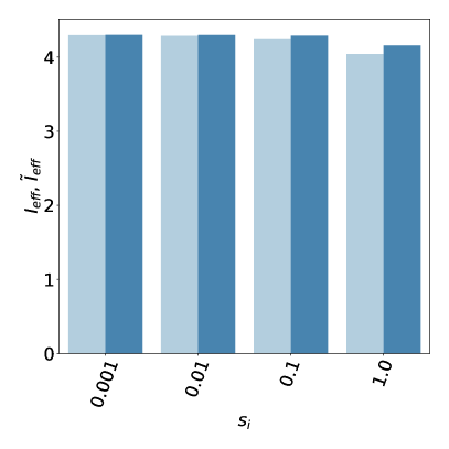
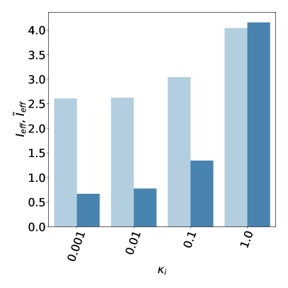
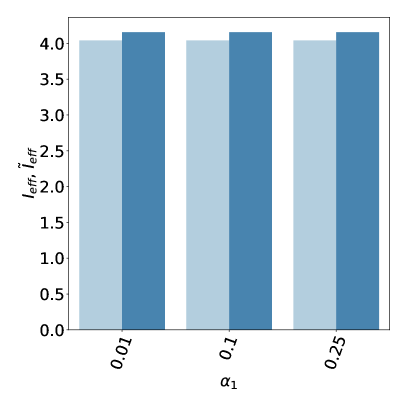
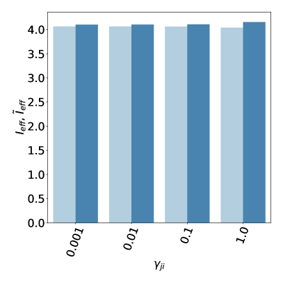
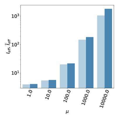
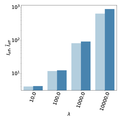
Figure 1. Efficiency indices for the smooth 3-network test case for different variations of the MPET material parameters $s_{i}$, $\kappa_{i}$, $\alpha_{i}$, $\gamma_{ji}$, $\mu$, and $\lambda$; energy-norm indices $I_{\rm eff}$ (light blue) and Bochner norm indices $\tilde{I}_{\rm eff}$ (middle blue). Numerical resolution parameters were kept fixed ($T=0.4$, $\tau=0.1$, $n=8$).

We also study how variations in the material parameters affect the effectivity of the error estimates, measured in terms of the effectivity index $I_{\rm eff}$ (6.1) with respect to the energy norm(s). We consider a set of default parameters: $\mu=1.0$, $\lambda=10.0$, $\alpha_{1}=0.25$, $\alpha_{2}=\alpha_{3}-\alpha_{1}$, $\alpha_{3}=0.5$, $s_{i}=\kappa_{i}=\gamma_{ji}=1.0$ for $i=1,2,3$, $j\not=i$, and subsequently independent variations in the material parameters representing increased stiffnesses $E$, reduced compressibilities $\nu$, lower transfer $\gamma$, lower hydraulic conductances $\kappa$, and lower specific storage coefficients $s$. Specifically, we consider $\alpha_{1}\in\{0.01,0.1,0.25\}$, $s_{i},\kappa_{i},\gamma_{ji}\in\{0.001,0.01,0.1,1.0\}$ for $i=1,2,3$, $j\not=i$, and $\mu\in\{1,10,100,1000,10000\}$, $\lambda\in\{10,100,1000,10000\}$. Both energy-norm and Bochner efficiency indices $I_{\rm eff}$ and $\tilde{I}_{\rm eff}$ for the different variations are shown in Figure 1.

The energy-norm efficiency indices $I_{\rm eff}$ are above 1 for all material variations considered. Variations in the specific storage coefficients, Biot-Willis coefficients and transfer coefficients have minimal effect on both the energy- and Bochner norm efficiency indices: the efficiency indices are $\sim 4$ for all variations in each of these parameters. For variations in the permeabilities $\kappa_{i}$, we observe some reduction in the energy-norm efficiency indices as the permeability is reduced (from $4.1$ to $2.6$), but that the index value stabilizes around $2.5$ for the smaller permeabilities. We observe similar behaviour for the Bochner-norm efficiency index, but with index values of $\sim 0.8$ for the smaller permeabilities, and thus efficiency indices below $1.0$. For the elastic parameters, the results are quite different. Both the energy-norm and Bochner efficiency indices increase substantially with increasing Lamé parameters $\mu$ and $\lambda$, though with Bochner efficiency indices increasing more.

Remark 6.1.

The boundedness of efficiency indices, e.g. $I_{\rm eff}$ and $\tilde{I}_{\rm eff}$, is canonically provided by the reverse inequality of Proposition 5.2, whereby the the error indicators are bounded above in terms of a constant times the norm of the discretization error. That is, one establishes

$$\eta_{1}+\eta_{2}+\eta_{3}+\eta_{4}\lesssim||u-u_{h\tau}||_{L^{\infty}(0,T;V_{a})} +||p-p_{h\tau}||_{L^{\infty}(0,T;L_{d})}$$

$$+||p-p_{h\tau}||_{L^{2}(0,T;V_{d})}+||p-\pi^{0}p_{h\tau}||_{L^{2}(0,T;V_{d})}.$$

If the constant of proportionality, in the above inequality, does not involve specific material parameters, then the efficiency indices are robust with respect to variations in those parameters. However, as in the case of the use of higher-order time discretizations, the general Euler-Galerkin elliptic-parabolic framework of Ern and Meunier [15] does not provide this bound and, as a result, its extension to the equations of generalized poroelasticity (MPET), presented herein, is limited in this same regard. The computational experiments of this section suggest that such an estimate will entail a constant of proportionality that scales strongly with both $\mu$ and $\lambda$.

7. Adaptive strategy: algorithmic considerations and numerical evaluation

We now turn to consider and evaluate two components of an overall adaptive strategy: (i) temporal adaptivity (only) and (ii) temporal and spatial adaptivity. Our choices for the adaptive strategy can be viewed in light of the observations on the convergence of $\eta_{1},\eta_{2},\eta_{3},\eta_{4}$ for the previous test case, as well as the following characteristics of MPET problems arising in e.g. biological applications:

• Mathematical models of living tissue are often associated with a wide range of uncertainty e.g. in terms of modelling assumptions, material parameters, and data fidelity. Simulations are therefore often not constrained by a precise numerical error tolerance, but rather by the limited availability of computational resources.

• Living tissue often feature heterogeneous material parameters, but typically with small jumps, and in particular smoother variations than e.g. in the geosciences. The corresponding MPET solutions are often relatively smooth.

• Even for problems with a small number of networks $J$ such as single or two-network settings, the linear systems to be solved at each time step are relatively large already for moderately coarse meshes.

In light of these points, our target is an adaptive algorithm robustly reducing the error(s) given limited computational resources. We therefore consider an error balancing strategy in which we adaptively refine time steps such that the estimated temporal and spatial contributions to the error is balanced, then refine the spatial mesh to reduce the overall error, and repeat. This approach to spatial adaptivity seeks to balance the computational gains associated with adaptively refined meshes and the computational and implementational overhead costs associated with more sophisticated time-space adaptive methods, see e.g. [1, 7]. While a full space-time adaptive algorithm could yield time-varying meshes of lower computational cost, the computational costs associated with finite element matrix assembly over separate meshes, and interpolation of discrete fields between different meshes are often substantial. Without time-varying meshes, the blocks of the MPET linear operator can be reused (using the time steps $\tau_{n}$ as weights) which may reduce assembly time, and potentially linear system solver times. We note though that there is ample room for more sophisticated time step control methods than we consider here, see e.g. [34] and related works.

7.1. Time adaptivity

We consider the time-adaptive scheme listed in Algorithm 1. Overall, for a given mesh $\mathcal{T}_{h}$, we step forward in time, evaluate (an approximation to) the error estimators at the current time step, compare the spatial and temporal contributions to the error estimators, and coarsen (or refine) the time step if the spatial (or temporal) error dominates.

1:Define adaptive parameters $\alpha_{\eta}\in[0,1)$ and $\beta\geq 1$, $\tau_{\max}>0$ and $\tau_{\min}\geq 0$.

2:Assume that a mesh $\mathcal{T}_{h}$ and an initial time step size $\tau_{0}$ is given. Set $t^{0}$ and set the time step iterator $n=0$.

3:while $t^{n}<T$ do

4:     while True do

5:         Set $n=n+1$.

6:         Set $t^{\ast}=t^{n-1}+\tau_{n}$, and solve (4.2) over $\mathcal{T}_{h}$ for $(u^{\ast}_{h},p^{\ast}_{h})$ with time step size $\tau_{n}$

7:         Compute error estimator approximations at the current time step

$$\eta_{1}^{n}=(\tau_{n}\eta^{n}_{p})^{\frac{1}{2}},\quad\eta_{2}^{n}=(\sup_{0\geq m\geq n}\eta^{m}_{u})^{\frac{1}{2}},\quad\eta_{3}^{n}=\tau_{n}(\eta_{u}^{n}(\delta_{t}))^{\frac{1}{2}},\quad\eta_{4}^{n}=(\tau_{n}\|p_{h}^{n}-p_{h}^{n-1}\|_{d}^{2})^{\frac{1}{2}},$$

8:         and set $\eta_{h}^{n}=\eta_{1}^{n}+\eta_{2}^{n}+\eta_{3}^{n}$, $\eta_{\tau}^{n}=\eta_{4}^{n}$.

9:         if $\eta_{\tau}^{n}\leq(1-{\color[rgb]{0,0,0}\alpha_{\eta}})\eta_{h}$ and $\beta\tau_{n}\leq\tau_{\max}$ then

10:              Set $t^{n}=t^{\ast}$, $(u^{n}_{h},p^{n}_{h})=(u^{\ast}_{h},p^{\ast}_{h})$, coarsen the next $\tau^{n+1}=\beta\tau^{n}$, and break loop.

11:         else if $\eta_{\tau}^{n}\geq(1+{\color[rgb]{0,0,0}\alpha_{\eta}})\eta_{h}^{n}$ and $\tau_{n}/\beta\geq\tau_{\min}$ then

12:              Discard the solution and refine the time step: set $t^{n}=t^{n-1}$, $n=n-1$, $\tau^{n}=\tau^{n}/\beta$.

13:         else

14:              Set $t^{n}=t^{\ast}$, $(u^{n}_{h},p^{n}_{h})=(u^{\ast}_{h},p^{\ast}_{h})$, $\tau^{n+1}=\tau^{n}$, and break loop.

15:         end if

16:     end while

17:end while

Algorithm 1 Time-adaptive algorithm

Evaluation of the time-adaptive algorithm on a smooth numerical test case

We evaluate Algorithm 1 using the numerical test case with smooth solutions defined over 3 networks as introduced in Section 6, the default material parameters, and different uniform meshes (defined by $2\times N\times N$ triangles as before). We also verified the adaptive solver by comparing the solutions at each time step and error estimators resulting from rejected coarsening and refinement (resulting in $\tau_{n}=0.2$ for each $n$) with the solutions and error estimators computed with a uniform time step ($\tau=0.2$). We let $T=1.0$, and considered an initial time step of $\tau_{0}=0.2$, adaptive weight ${\color[rgb]{0,0,0}\alpha_{\eta}}=0$, a coarsening/refinement factor $\beta=2$, and time step bounds $\tau_{\max}=T$ and $\tau_{\min}=0.0$.

The discrete times $t^{n}$ resulting from the adaptive algorithm, error estimators $\eta_{h}^{n}$ and $\eta_{\tau^{n}}$ are shown in Figure 2 for different uniform mesh resolutions. For $N=8$ (Figure 2(a)), we observe that the adaptive algorithm estimates the initial time step of $0.2$ to be unnecessarily small in light of the dominating spatial error, and coarsens the time step to $0.4$ before quickly reaching the end of time ($T$). The $\|u-u_{h\tau}\|_{L^{\infty}}$, $\|p-p_{h\tau}\|_{L^{\infty}}$, and $\|p-p_{h\tau}\|_{L^{2}}$ errors are $4.61\times 10^{-3}$, $3.86\times 10^{-2}$ and $6.83\times 10^{-1}$. For comparison, with a uniform time step $\tau=0.2$, the $\|u-u_{h\tau}\|_{L^{\infty}}$, $\|p-p_{h\tau}\|_{L^{\infty}}$, $\|p-p_{h\tau}\|_{L^{2}}$, and $\|p-\pi^{0}p_{h\tau}\|_{L^{2}}$ (as listed in Table 1) are $4.71\times 10^{-3}$, $4.38\times 10^{-2}$, $4.96\times 10^{-1}$, and $1.33$ respectively, and thus the errors with the adaptively defined coarser time step are very comparable - as targeted by our error balancing principle. The picture changes for $N=16$ (Figure 2(b)), in this case the temporal error initially dominates the spatial error, and the time step is reduced substantially initially before a subsequent increase and plateau at $0.1-0.2$. The value of the adaptive error estimator $\eta_{4}$ is lower than for the uniform solution ($1.23$ vs $2.17$), but the exact errors are comparable between the uniform and adaptive scheme in this case. By setting $\tau_{\min}=\tau^{0}/4$, the unnecessarily high initial time step refinement is limited (Figure 2(c)), and again comparable errors as for the uniform time step are observed. For higher spatial resolution and thus lower spatial errors ($N=32$), similar observations hold (Figure 2(d)), but now the adaptive solutions approximately halve the exact errors compared to the uniform $\tau^{0}=0.2$ case (as expected). We conclude that the time adaptive scheme efficiently balances the temporal and spatial error, but does little for reducing the overall error – as the spatial error dominates this case. For $N=64$ and the same configurations, the adaptive time step reduces to the minimal threshold $\tau_{0}/4=0.05$ and remains there until end of time $T$, with the expected quartering of the exact errors compared to the $\tau_{0}=0.2$ case (and the first order accuracy of the temporal discretization scheme).

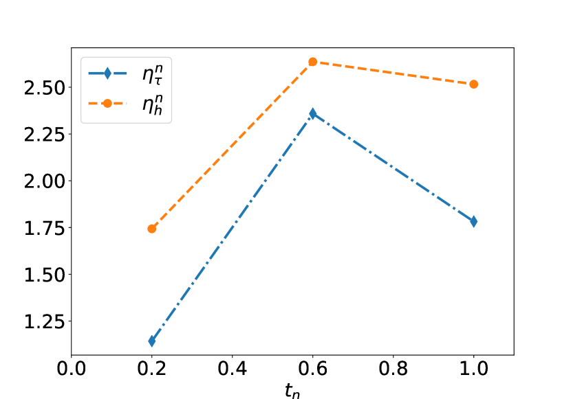
(a) $N=8$.

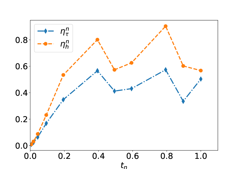
(b) $N=16$.

(c) $N=16$ and $\tau_{\min}=\tau^{0}/4$.

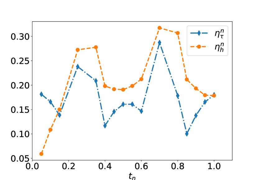
(d) $N=32$ and $\tau_{\min}=\tau^{0}/4$.

Figure 2. Evaluation of adaptive time stepping for a smooth numerical test case, given uniform meshes and different adaptive parameter configurations. All plots show the approximated error estimators $\eta_{h}^{n}$ and $\eta_{\tau}^{n}$ at each time step versus adaptive times $t^{n}$.

7.2. Spatial adaptivity

For the spatial adaptivity, we use adaptive mesh (h-)refinement based on local error indicators $\{\eta_{K}\}_{K\in\mathcal{T}_{h}}$ derived from the global error estimators (5.20). In light of the theoretical and empirical observation that $\eta_{4}$ primarily contributes to the temporal error, we will rely on local contributions to $\eta_{1},\eta_{2}$ and $\eta_{3}$ only for the local error indicators. Specifically, we will let

$$\eta_{K}=\eta_{1,K}+\eta_{2,K}+\eta_{3,K}$$ (7.1)

where

$$\eta_{1,K}=\left(\sum_{n=1}^{N}\tau_{n}\eta_{p,K}^{n}\right)^{\frac{1}{2}},\quad\eta_{2,K}=\left(\sup_{0\leq n\leq N}\eta_{u,K}^{n}\right)^{\frac{1}{2}},\quad\eta_{3,K}=\sum_{n=1}^{N}\tau_{n}\left(\eta_{u,K}^{n}(\delta_{t})\right)^{\frac{1}{2}}.$$ (7.2)

for each $K\in\mathcal{T}_{h}$. The complete space-time adaptive algorithm is given in Algorithm 2. We here choose to use Dörfler marking [13] or a maximal marking strategy in which the $\gamma_{M}$ of the total number of cells with the largest error indicators are marked for refinement, but other marking strategies could of course also be used.

1:Assume that an error tolerance $\epsilon$ and/or a resource limit $L$ and an initial mesh $\mathcal{T}=\mathcal{T}_{h}^{0}$ are given. Set a marking fraction parameter $\gamma_{M}\in(0,1]$.

2:while True do

3:     Set the parameters ($\tau_{0},{\color[rgb]{0,0,0}\alpha_{\eta}},\beta,\tau_{\max},\tau_{\min}$) required by Algorithm 1.

4:     Solve (4.2) over $\mathcal{T}$ via the time-adaptive scheme defined by Algorithm 1.

5:     Estimate the error $\eta=\eta_{1}+\eta_{2}+\eta_{3}+\eta_{4}$ where $\eta_{i}$ for $i=1,2,3,4$ are given by (5.20).

6:     if $\eta<\epsilon$ then

7:         Break

8:     end if

9:     Compute spatial error estimators $\eta_{K}$ for $K\in\mathcal{T}$ via (7.1).

10:     From $\{\eta_{K}\}$, define Boolean refinement markers $\{y_{K}\}_{K\in\mathcal{T}_{h}}$ via Dörfler or maximal marking (with $\gamma_{M}$).

11:     Refine $\mathcal{T}$ (locally) based on the markers $\{y_{K}\}$.

12:     if $|\mathcal{T}|>L$ then

13:         Break

14:     end if

15:end while

Algorithm 2 Space-time adaptive algorithm

Remark 7.1.

In Algorithm 2, we suggest adapting the mesh in each outer iteration via only (local) mesh refinements. One could equally well consider a combination of local mesh refinement and coarsening, and/or other adaptive mesh techniques such as r-refinement. Indeed, this could be particularly relevant in connection with complex geometries, for which the initial mesh may be overly fine (in terms of approximation power) in geometrically involved local regions.

Evaluation of the space-time-adaptive algorithm on a smooth numerical test case

We evaluate Algorithm 2 using the numerical test case with smooth solutions defined over 3 networks as introduced in Section 6 with the default material parameters. As this is a smooth test case in a regular domain, we expect only moderate efficiency improvements (if any) from adaptive mesh refinement, and therefore primarily evaluate the accuracy of the error estimators on adaptively refined meshes and the balance between temporal and spatial adaptivity.

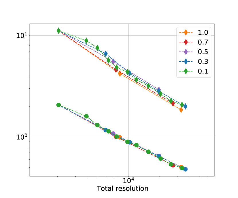
(a) Approximation error $E$ (dots) and error estimates $\eta$ (diamonds) versus total resolution ($|\mathcal{T}|\times N$) at different adaptive iterations with a uniform timestep $\tau=1/64$ for different Dörfler marking fractions ($1.0,0.7,0.5,0.3,0.1$).

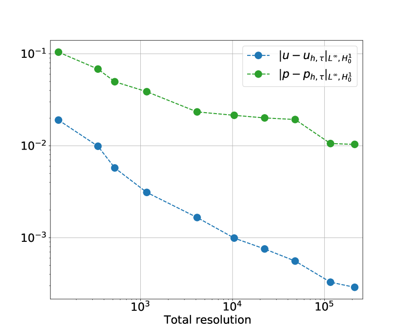
(b) Displacement and pressure approximation errors under adaptive refinement as generated by the space-time adaptive algorithm with $\tau_{0}=T/4$, ${\color[rgb]{0,0,0}\alpha_{\eta}}=0.3$, $\beta=2.0$, $\gamma_{M}=0.3$, $\tau_{\max}=\tau_{0}$, $\tau_{\min}=\tau_{0}/16$, and $L\approx 8000$.

(c) Error indicators on final mesh refinement level with yellow values indicating high error indicators (colormap: viridis) (same parameters as in Figure 3(b)).

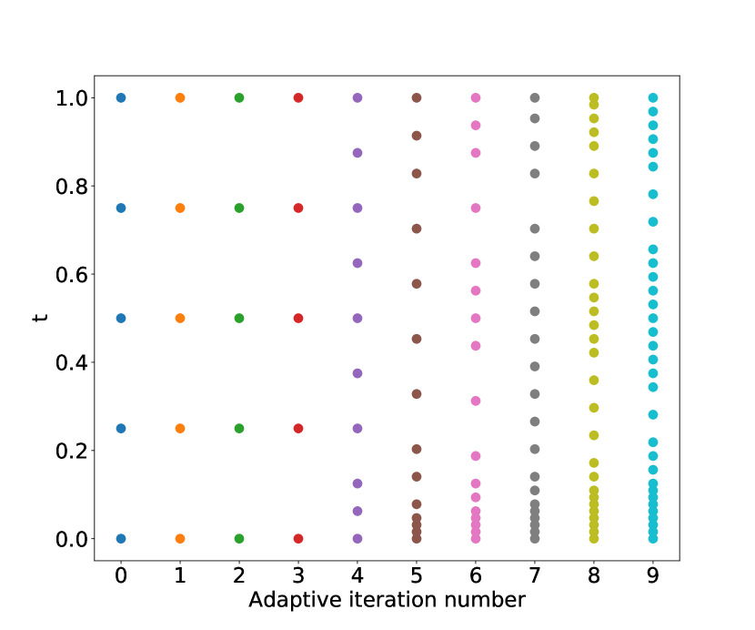
(d) Discrete times (and time steps) generated by the space-time adaptive algorithm (same parameters as in Figure 3(b)).

Figure 3. Evaluation of the space-time adaptive algorithm on a smooth test case.

We set $T=1.0$, $\tau_{0}=0.5$, and begin with a $2\times 4\times 4$ mesh of the unit square as $\mathcal{T}_{h}^{0}$. We set $\epsilon=0$, but instead prescribe a resource tolerance $L$. We first set a fine initial time step $\tau_{0}=T/64$, and let $\beta=2.0$, ${\color[rgb]{0,0,0}\alpha_{\eta}}=0.3$, $\tau_{\min}=\tau_{0}/16$, and $\tau_{\max}=\tau_{0}$ in Algorithm 1. We note that a Dörfler marking fraction $\gamma_{M}$ of $1.0$ yields a series of uniformly refined meshes. For marking fractions between 0.0 and 1.0, we obtain adaptively refined meshes, yet for this test case, the time step remains uniform throughout the adaptive loop. The resulting errors and error estimates at each adaptive refinement iteration are shown in Figure 3(a). We observe that the errors decay as expected, and that the error estimates provide upper bounds for the errors $E$ at each refinement level for all marking fractions tested.

We next let $\tau_{0}=T/4$ and $\gamma_{M}=0.3$ (and all other parameters as before), and consider the results of the adaptive algorithm (Figure 3(b)–3(d)). We find that the adaptive algorithm keeps the initial time step and refines the mesh only for the first 4 iterations, which substantially reduces the $L^{\infty}H^{1}_{0}$ displacement approximation error and moderately reduces the $L^{\infty}H^{1}_{0}$ pressure approximation error. For the next iterations, both the mesh and the time step is refined. The pressure errors seem to plateau before continuing to reduce given sufficient mesh refinement, while the displacement errors steadily decrease.

8. Adaptive brain modelling and simulation

We turn to consider a physiologically and computationally realistic scenario for simulating the poroelastic response of the human brain. Human brains form highly non-trivial, non-convex domains characterized by narrow gyri and deep sulci, and as such represent a challenge for mesh generation algorithms. Therefore, brain meshes are typically constructed to accurately represent the surface geometry, without particular concern for numerical approximation properties. We therefore ask whether the adaptive algorithm presented here can effectively and without further human intervention improve the numerical approximation of key physiological quantities of interest starting from a moderately coarse initial mesh and initial time step.

Specifically, we let $\Omega$ be defined by a subject-specific left brain hemisphere mesh (Figure 4(a)) generated from MRI-data via FreeSurfer [17] and SVMTK as described e.g. in [26]. The domain boundary is partitioned in two main parts: the semi-inner boundary enclosing the left lateral ventricle $\partial\Omega_{v}$ and the remaining boundary $\partial\Omega_{s}$ (Figure 4(b)).

Over this domain, we consider the MPET equations (3.3) with $J=3$ fluid networks representing an arteriole/capillary network ($j=1$), a low-pressure venous network ($j=2$), and a perivascular space network ($j=3$). We assume that the two first networks are filled with blood, while the third network is filled with cerebrospinal fluid (CSF).

8.1. Pulsatility driven by fluid influx

We consider a scenario in which fluid influx is represented by a pulsatile uniform source in the arteriole/capillary network ($j=1$):

$$g_{1}(x,t)=g_{1}(t)=\frac{1}{2}(1-\cos(2\pi t)),$$ (8.1)

while we set $g_{2}=g_{3}=f=0$. From the arteriole/capillary network, fluid can transfer either into the venous network or into the perivascular network with rates $\gamma_{12},\gamma_{13}>0$, while $\gamma_{23}=0$. All material parameters are given in Table 3.

Parameter	Value	Note
$E$ (Young’s modulus)	$1.642\times 10^{3}$ Pa	[10] (gray/white average)
$\nu$ (Poisson’s ratio)	$0.497$	$\ast$
$s_{1}$ (arteriole storage coefficient)	$2.9\times 10^{-4}$ Pa-1	[19] (arterial network)
$s_{2}$ (venous storage coefficient)	$1.5\times 10^{-5}$ Pa-1	[19] (venous network)
$s_{3}$ (perivascular storage coefficient)	$2.9\times 10^{-4}$ Pa-1	[19] (arterial network)
$\alpha_{1}$ (arteriole Biot-Willis parameter)	$0.4$	$\ast$
$\alpha_{2}$ (venous Biot-Willis parameter)	$0.2$	$\ast$
$\alpha_{3}$ (perivascular Biot-Willis parameter)	$0.4$	$\ast$
$\kappa_{1}$ (arteriole hydraulic conductance)	$3.75\times 10^{-2}$ mm2 Pa-1 s-1	$k_{1}$/$\mu_{1}$, see below
$\kappa_{2}$ (venous hydraulic conductance)	$3.75\times 10^{-2}$ mm2 Pa-1 s-1	$k_{2}$/$\mu_{1}$, see below
$\kappa_{3}$ (perivascular hydraulic conductance)	$1.43\times 10^{-1}$ mm2 Pa-1 s-1	$k_{3}$/$\mu_{3}$, see below
$\gamma_{12}$ (arteriole-venous transfer)	$1.0\times 10^{-3}$ Pa-1 s-1	$\ast$
$\gamma_{13}$ (arteriole-perivascular transfer)	$1.0\times 10^{-4}$ Pa-1 s-1	$\ast$
$C$ (environment compliance)	$10$	$\ast$
$R$ (environment resistance)	$79.8$ Pa / (mm3 / s)	[38]
$k_{1}$ (arteriole permeability)	$1.0\times 10^{-10}$ m2	[19] (arterial network)
$k_{2}$ (venous permeability)	$1.0\times 10^{-10}$ m2	[19] (venous network)
$k_{3}$ (perivascular permeability)	$1.0\times 10^{-10}$ m2	Estimate, vascular permeability
$\mu_{1}$ (blood dynamic viscosity)	$2.67\times 10^{-3}$ Pa s	[19] (arterial network)
$\mu_{3}$ (CSF dynamic viscosity)	$6.97\times 10^{-4}$ Pa s	[12] (water at body temperature)

Table 3. Material parameters corresponding to a human brain at body temperature. The hydraulic conductances $\kappa$ are defined in terms of the permeabilities and the fluid viscosities $\kappa_{j}=k_{j}/\mu_{j}$, $\mu_{2}=\mu_{1}$. Values marked by the $\ast$ are estimates, yielding physiologically reasonable brain displacements, fluid pressures, and fluid velocities.

In terms of boundary conditions for the momentum equation, we set

$$u =0\quad \text{ on the outer boundary }\partial\Omega_{s},$$ (8.2a)

$$(\sigma-\textstyle\sum_{j}\alpha_{j}p_{j}I)\cdot n =-p_{\rm csf}\,n\quad \text{ on the inner boundary }\partial\Omega_{v}.$$ (8.2b)

for a spatially-constant $p_{\rm csf}$ to be defined below. For the arteriole space, we assume no boundary flux:

$$\operatorname{\nabla}p_{1}\cdot n=0\quad\text{ on }\partial\Omega.$$ (8.3)

We assume that the venous network is connected to a low (zero) pressure compartment and set:

$$p_{2}=0\quad\text{ on }\partial\Omega.$$ (8.4)

We assume that the perivascular space is in direct contact with its environment, and set:

$$p_{3}=p_{\rm csf}\quad\text{ on }\partial\Omega.$$ (8.5)

Last, we model $p_{\rm csf}$ via a simple Windkessel model at the boundary:

$$C\dot{p}_{\rm csf}=Q-\frac{p_{\rm csf}}{R}$$ (8.6)

with compliance $C$ and a resistance $R$ (see Table 3), and where $Q$ is the outflow: $Q=\int_{\partial\Omega}u\cdot n\,\mathrm{d}s$. After an explicit time discretization, we define at each time step

$$Cp_{\rm csf}^{n+1}=\tau_{n}Q^{n}+(C-\frac{\tau_{n}}{R})p_{\rm csf}^{n},$$ (8.7)

and use (8.7) in (8.2) and (8.5). Finally, we let all fields start at zero. We let $T=2.0$ corresponding to two cardiac cycles, and an initial time step of $\tau_{0}=0.1$.

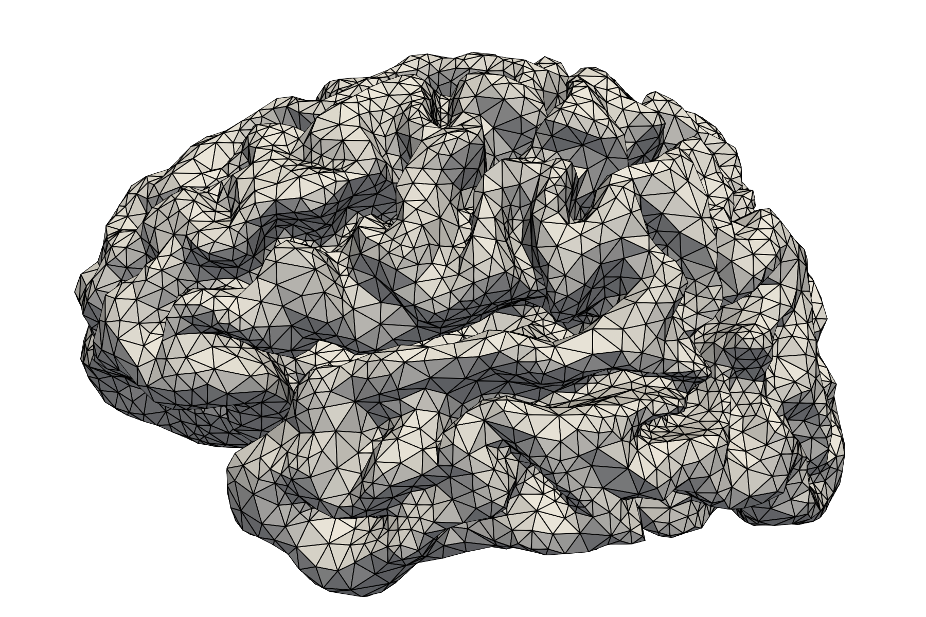
(a) Initial mesh of a brain hemisphere (sagittal view, along positive x-axis) with 20911 cells and 6325 vertices, and a volume of $4.37\times 10^{5}$ mm³.

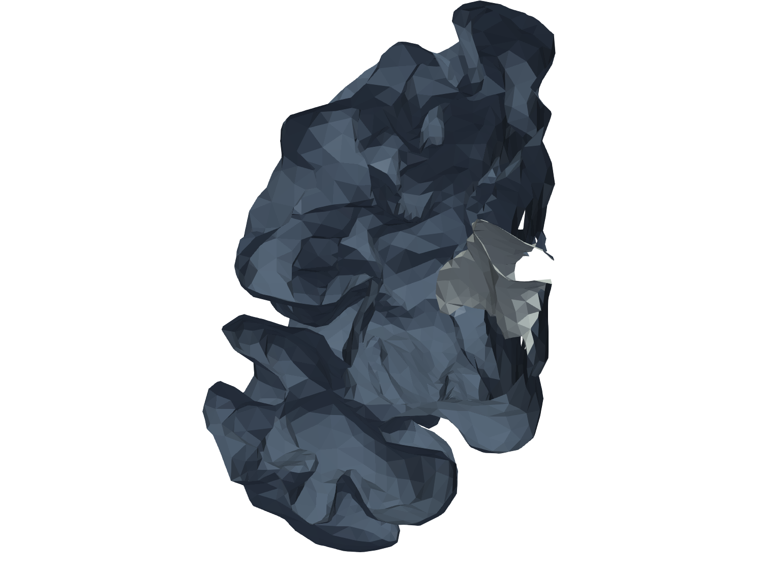
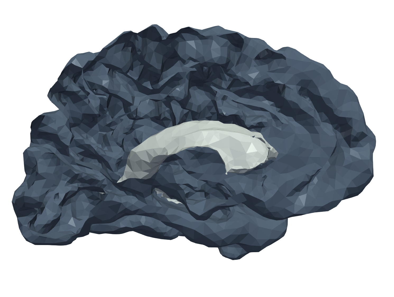
(b) Illustration of the semi-inner ventricular boundary (in white), coronal and sagittal clips (view from the y- and negative x-axes, respectively).

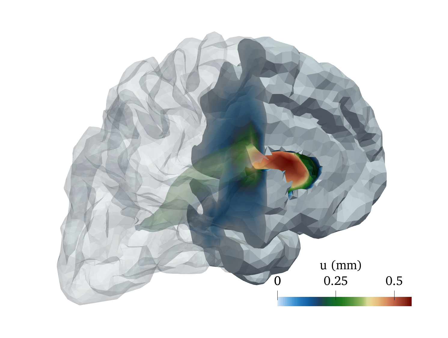
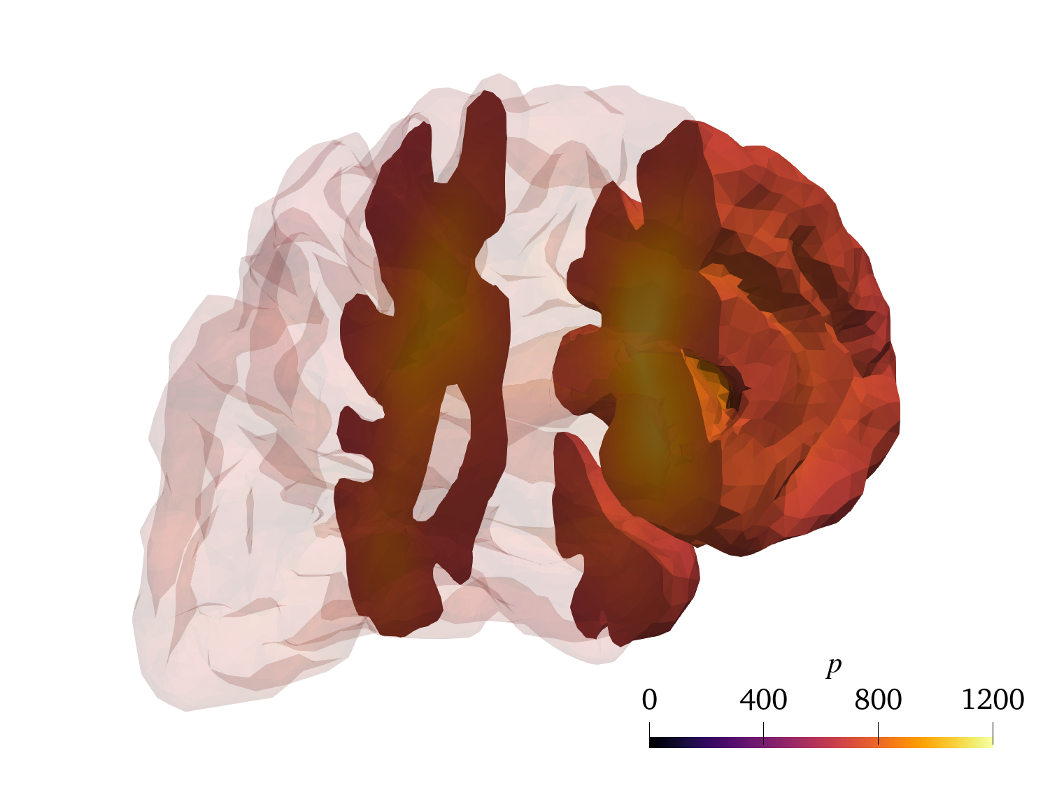
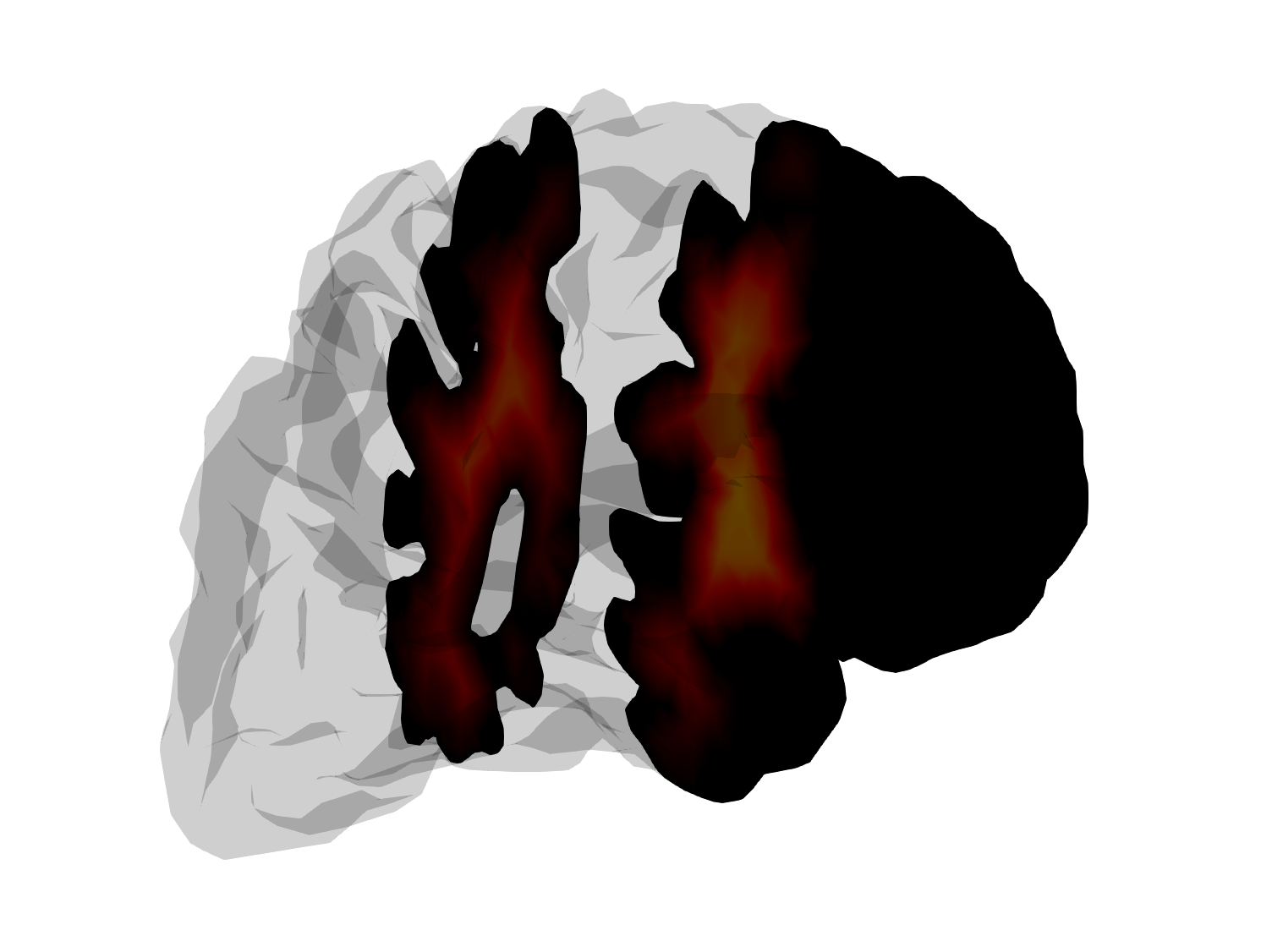
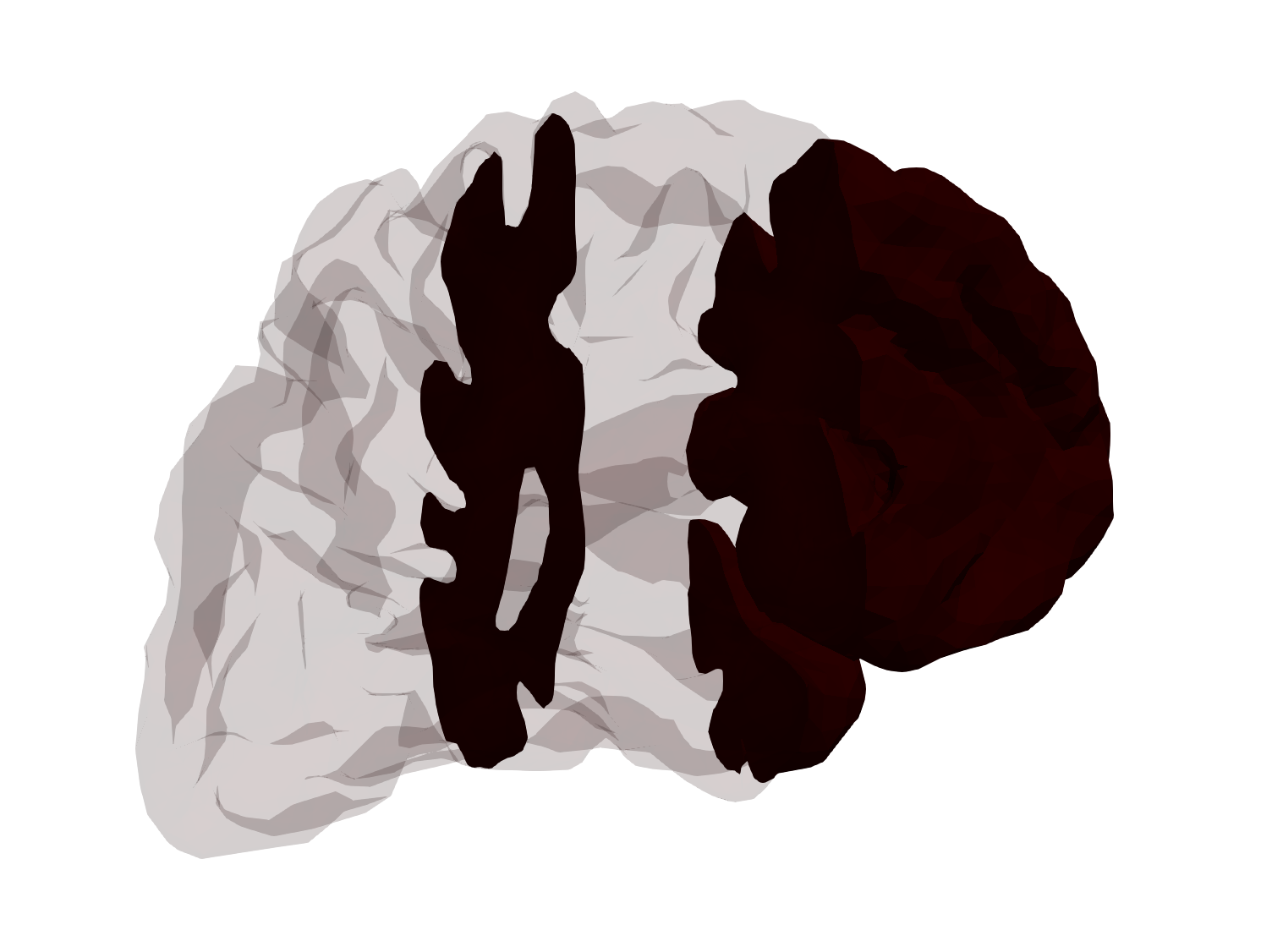
(c) Left to right, top to bottom: Displacement $u$ magnitude, arteriole/capillary pressure $p_{1}$, venous pressure $p_{2}$, and perivascular pressure $p_{3}$ at peak displacement ($T=1.7$).

Figure 4. The human brain as a poroelastic medium: meshes, boundaries, and snapshots of solution fields.

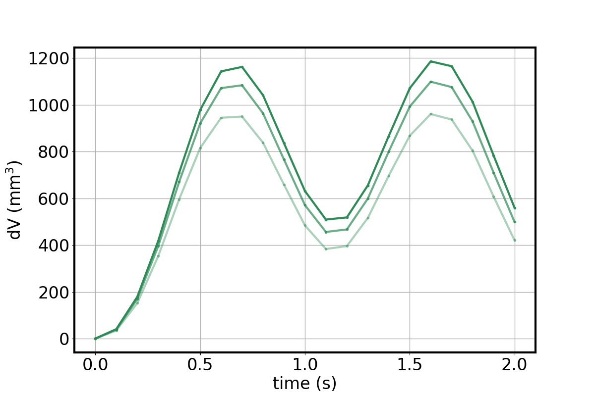
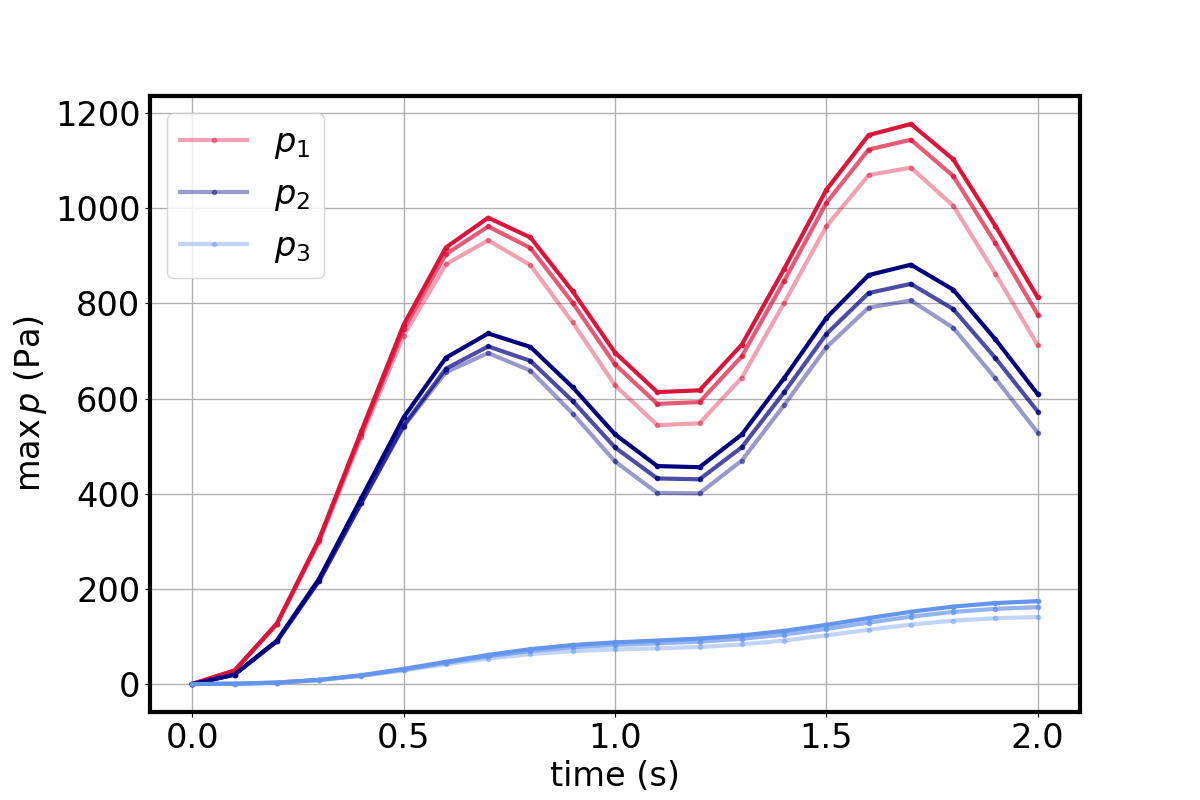
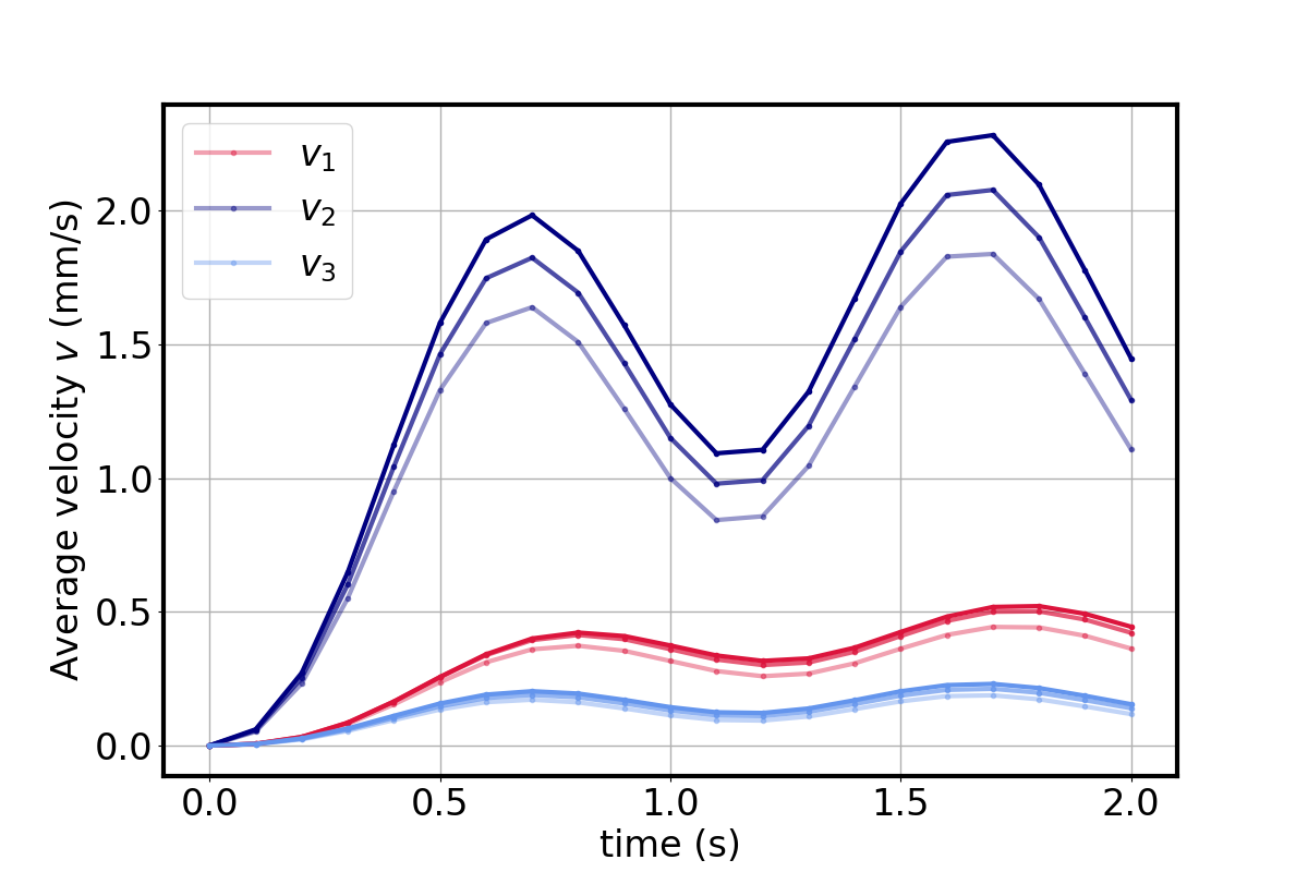
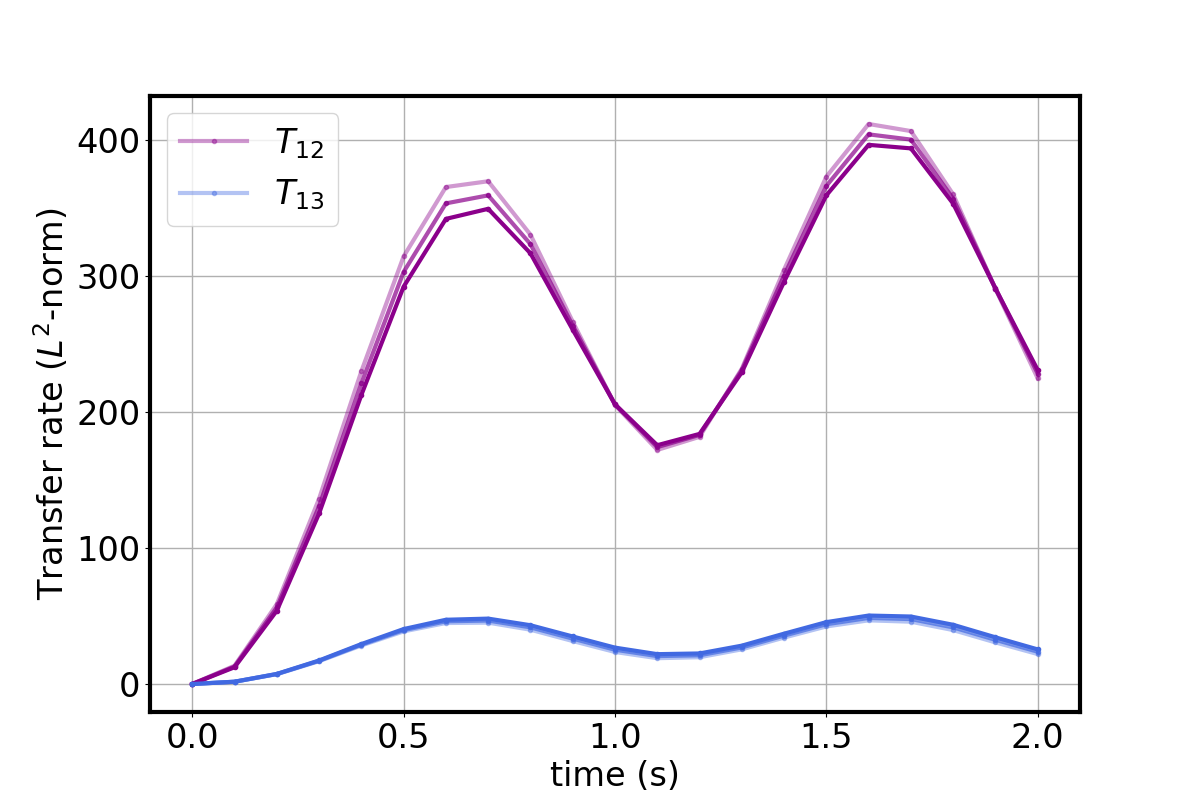
Figure 5. Left to right, top to bottom: Volume change $\textrm{d}V$, peak pressure $p_{i}$ and average velocity $v_{i}$ for $i=1,2,3$ and integrated transfer rates $T_{12}$ and $T_{13}$ over time for a series of adaptively refined meshes (a1, a2, a3). The opacity indicates the adaptive level: the more opaque, the finer the mesh.

The given fluid influx induces pulsatile tissue displacements and pressures in the different networks with varying temporal and spatial patterns (Figure 4(c), Figure 5). The brain hemisphere expands and contracts with peak changes in volume

$$\textrm{dV}=\int_{\Omega}\operatorname{\mathrm{div}}u\,\mathrm{d}x,$$

of up to 1200 mm³. The largest displacements occur around the lateral ventricle with peak displacement magnitudes of $\approx$0.5 mm. The arteriole/capillary pressure varies in space and time with a peak pressure $\max p_{1}$ of up to 1200 Pa, a pressure pulse amplitude $\Delta p_{1}$ of $\approx$ 560 Pa and a pressure difference in space of $\approx$ 400 Pa. The venous pressure field show similar patterns, though with lower temporal variations and higher spatial variability inducing higher venous blood velocities of above 2.0 mm/s (Figure 5). The perivascular pressure shows a steady increase of up to $\approx$ 200 Pa at $T=2.0$, but only moderate pulsatility and lower fluid velocities than both the arteriole/capillary and venous networks.

	#cells	$h_{\min}$	$h_{\max}$	#dofs	$\textrm{d}V$	$\Delta\textrm{d}V$	$\max p_{1}$	$\Delta p_{1}$	$\max v_{2}$	$\Delta v_{2}$
a1	20911	1.9	13.8	135774	961	577	1086	541	1.84	0.99
a2	66849	0.86	12.8	364416	1099	643	1144	555	2.08	1.10
a3	198471	0.43	11.4	1021749	1186	677	1177	564	2.28	1.19
u2	167288	0.7	9.8	922350	1162	668	1160	559	2.24	1.18

(a) Quantities of interest on the initial mesh (a1) and two adaptive refinement levels (a2, a3) and after uniform refinement (u2). Each row gives the number of mesh cells (#cells), minimal and maximal cell size $h_{\min}$, $h_{\max}$ (mm), the number of degrees of freedom per time step (# dofs), the computed peak volume change of the domain $\textrm{d}V$ (mm³), and pulsatile volume change amplitude $\Delta\textrm{d}V$ (mm³), peak arteriole/capillary pressure $\max p_{1}$ (Pa) and its pulsatile amplitude $\Delta p_{1}$ (Pa), peak venous fluid velocity $\max v_{2}$ (mm/s) and its pulsatile amplitude $\Delta v_{2}$ (mm/s).

	$\eta_{1}$	$\eta_{2}$	$\eta_{3}$	$\eta_{4}$	$\eta$
a1	$5.6\times 10^{3}$	$5.7\times 10^{5}$	$1.6\times 10^{6}$	$2.9\times 10^{3}$	$2.2\times 10^{6}$
a2	$4.6\times 10^{3}$	$2.7\times 10^{5}$	$7.8\times 10^{5}$	$2.9\times 10^{3}$	$1.1\times 10^{6}$
a3	$3.5\times 10^{3}$	$1.3\times 10^{5}$	$3.9\times 10^{5}$	$2.9\times 10^{3}$	$5.0\times 10^{5}$

(b) Computed error estimate $\eta$ and its partial contributions $\eta_{1},\eta_{2},\eta_{3},\eta_{4}$ (see cf. (5.20)) for the series of adaptively refined brain meshes (a1, a2, a3).

Table 4.

The local error indicators $\{\eta_{K}\}_{K}$ as defined by (7.1) show substantial local error contributions with substantial spatial variation (Figure 6): the values range from the order of $10^{3}$ to $10^{9}$ on the initial mesh $\mathcal{T}_{h}^{0}$. This large variation in error indicator magnitude makes the choice of marking strategy important: the Dörfler marking strategy would lead to the marking of perhaps only a handful of cells in this case as the local error indicators for a few cells would easily add up to a significant percentage of the total error. Therefore, we instead choose to employ a maximal marking strategy with a marking fraction $\gamma_{M}=0.03$ for this test scenario.

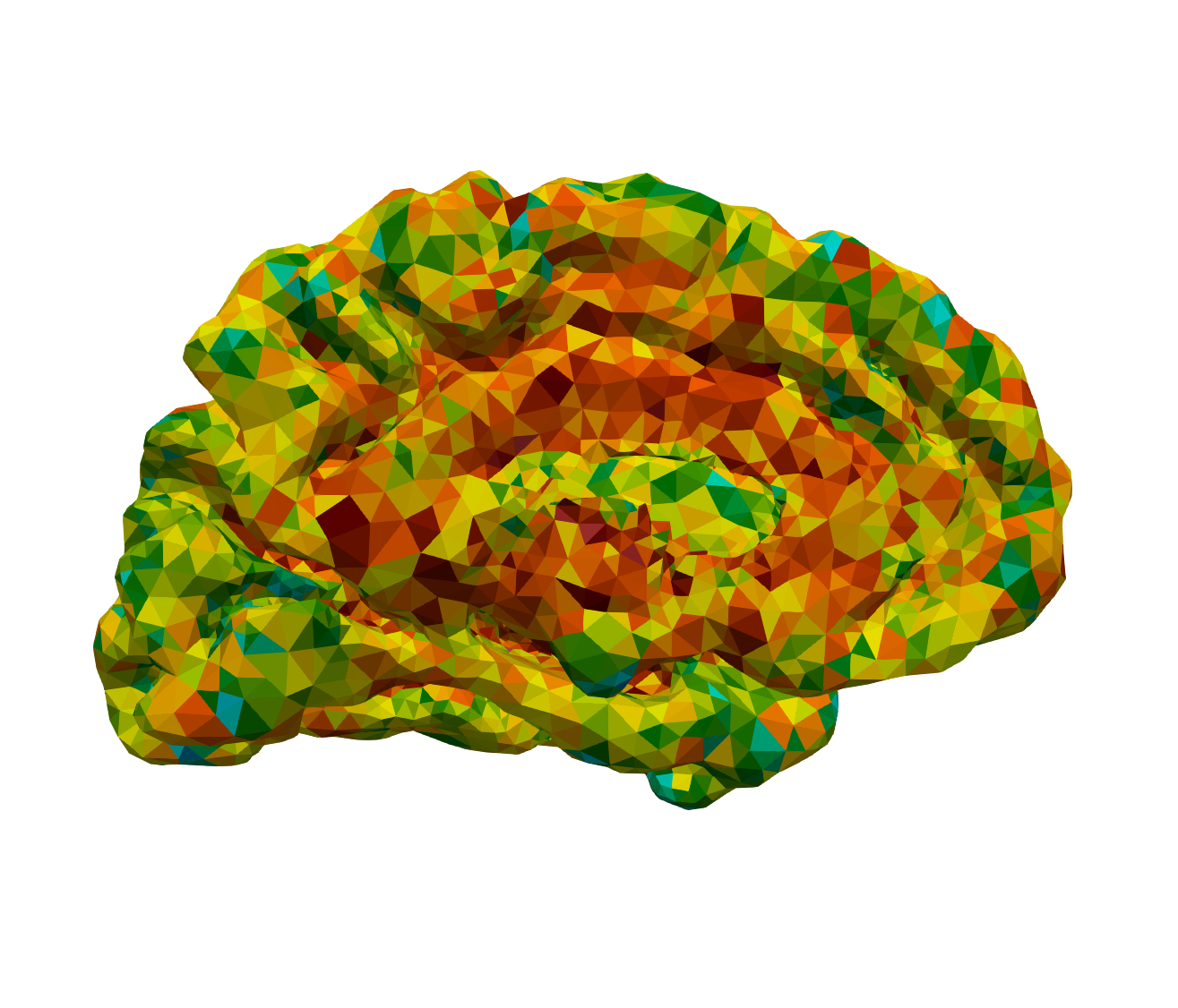
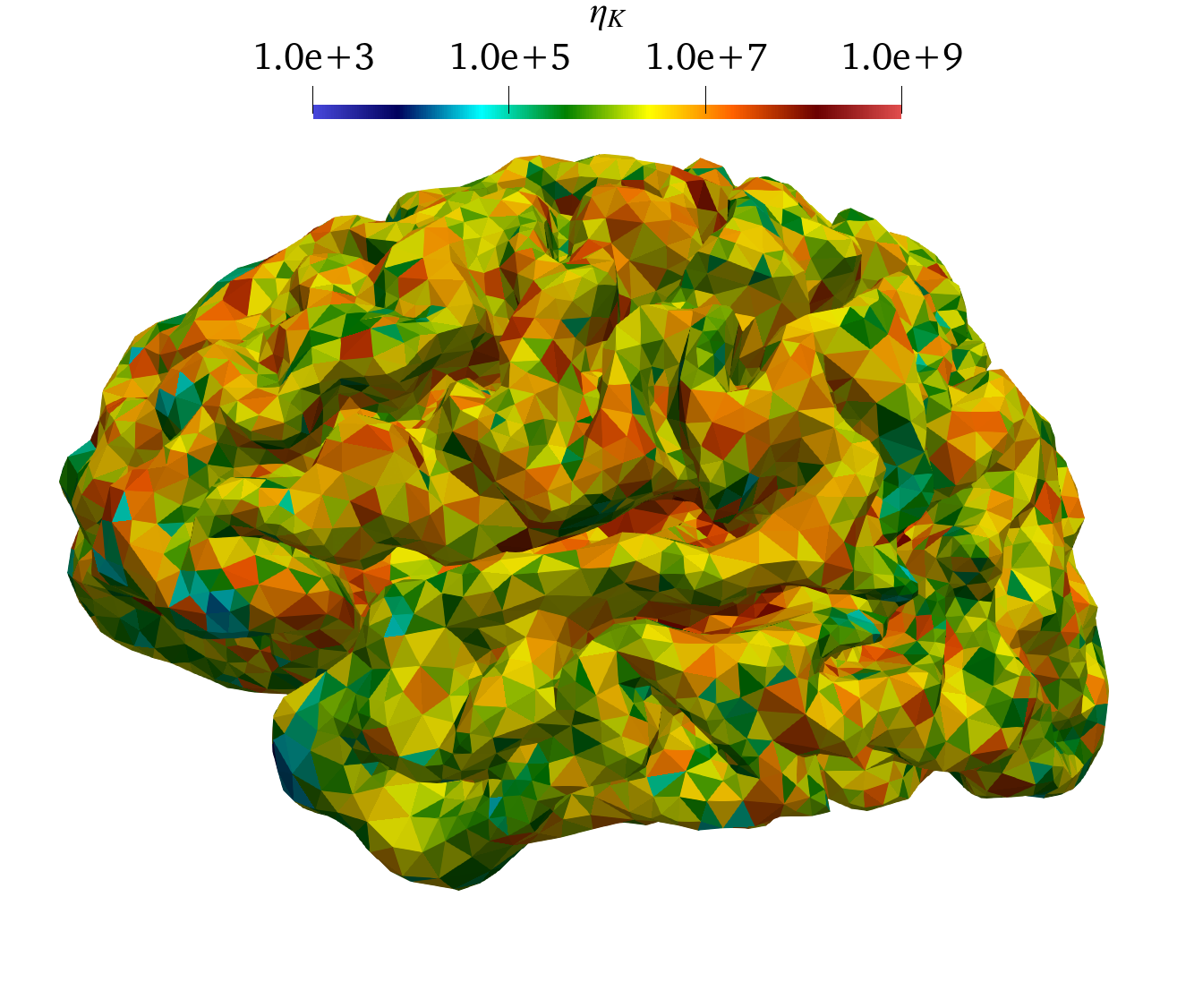
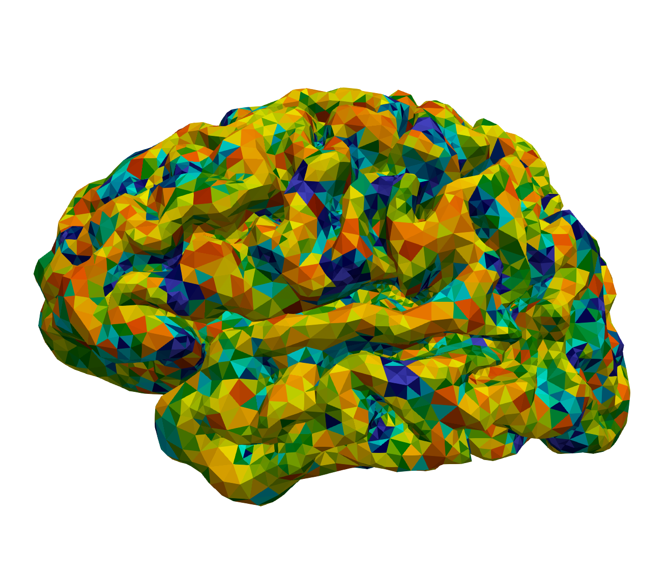
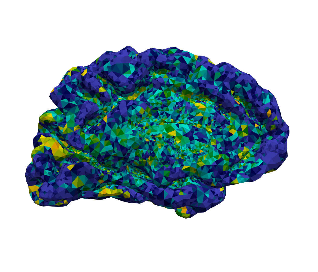
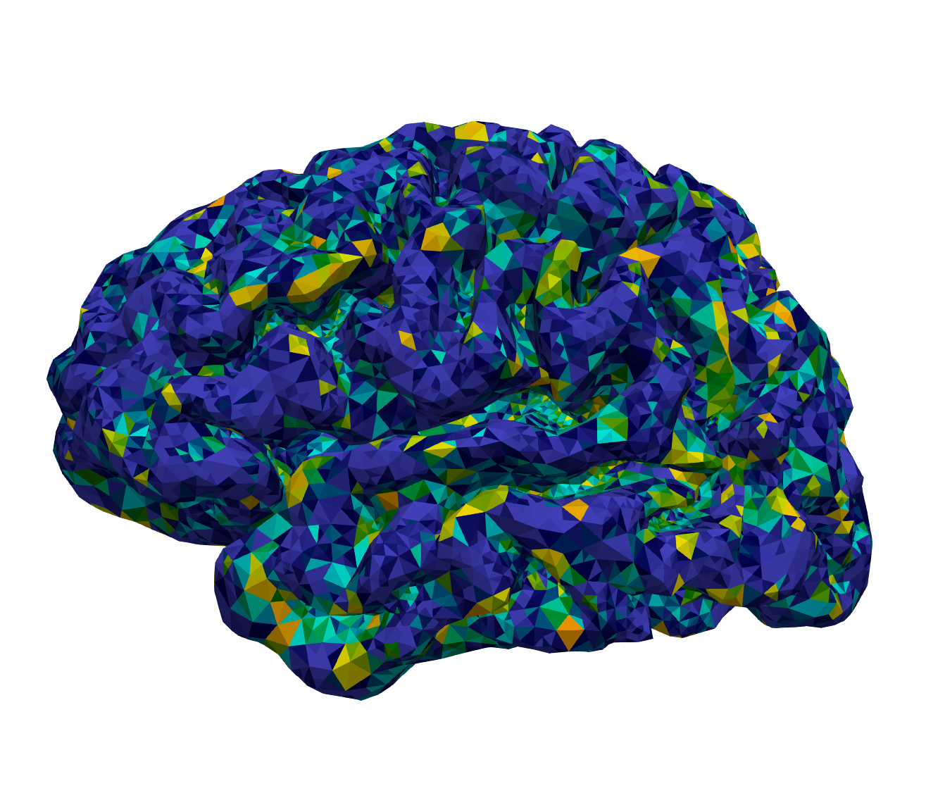
Figure 6. Error indicators $\{\eta_{K}\}_{K}$ for three levels of adaptive refinement $\mathcal{T}_{h}^{0},\mathcal{T}_{h}^{1},\mathcal{T}_{h}^{2}$ the brain simulation scenario. Refinement levels from top to bottom (a1, a2, a3), sagittal views from right and left on the left and right.

The adaptive algorithm yields locally refined meshes with around 67 000 cells after one refinement and 198 000 cells after two (Table 4(a)). The error estimates cf. (5.20) decrease with the adaptive refinement (Table 4(b)). The contribution from $\eta_{2}$ and $\eta_{3}$ dominates the error estimate, and both of these as well as the total error estimate $\eta$ seem to halfen for each adaptive refinement level. We also note that in this simulation scenario, for all time steps $n$ and refinement levels, the spatial error contribution $\eta_{h}^{n}$ dominates the temporal contribution $\eta_{\tau}^{n}$ cf. Algorithm 1. Thus, the adaptive algorithm does not refine the time step and the uniform initial time step of $\Delta t=0.1$ is kept throughout.

We also inspect the computed quantities of physiological interest (Table 4(a)). Using the uniform refinement as an intermediate reference value, we observe that the adaptive algorithm seems to produce more accurate estimates of these quantities of interest even after a single adaptive refinement, and that the quantities of interest after two refinements are more accurate than those of a uniform refinement. The adaptive procedure is therefore able to drive more accurate computation of quantities of interest at a lower or comparable cost as uniform refinement.

Finally, we observe that a single uniform refinement yields a mesh with around 167 000 cells (Table 4(a)). Thus, even with a small marking fraction of 3%, the mesh growth in each adaptive iteration is substantial. In the Plaza algorithm [28] and other similar conforming mesh refinement algorithms, both cells marked for refinement as well as neighboring cells will be refined to avoid mesh artefacts such as hanging nodes. Therefore, the domain geometry and initial mesh connectivity may strongly influence the adaptive mesh growth, and mesh growth may be more rapid than anticipated, especially in 3D. A more targeted adaptivity and more gradual growth could possibly be achieved with even lower marking fractions, though in the current case the propagation of cell refinement to neighboring cells seems to dominate. In any case, allowing for meshes with hanging nodes could be an effective albeit more disruptive strategy for reducing the computational complexity.

8.2. Pulsatility driven by boundary pressure

We also consider an alternative, more localized, scenario in which, instead of considering a Windkessel model for the CSF pressure and the directly coupled PVS pressure $p_{3}$, we directly prescribe a variation in the boundary PVS pressure. Concretely, we set

$$p_{\rm csf}=-2\times 133\sin(2\pi t)$$ (8.8)

and thus boundary CSF pressure variations of up to $\pm 2\times 133$ Pa (corresponding to approx. $\pm 2$ mmHg) in each cycle. In this scenario, we set the bulk fluid influx to zero ($g_{1}=g_{2}=g_{3}=0.0$). We consider otherwise the same experiments as in Section 8.1 and the same adaptive parameters. Also for this case, we observe that the adaptive refinement – even with a small marking fraction and maximal marking yields non-localized marking patterns and a relatively rapid growth in the number of mesh cells. Three adaptive refinements yields meshes with $20\,911$, $68\,608$ and $197\,975$ cells and no refinement of the time steps; numbers which are comparable with the previous case.

These results corroborate the observation that the adaptive algorithm drives distributed mesh refinement, and that the spatial errors overall dominate. Moreover, further studies may consider finer initial meshes and further refinements. A prerequisite for this would be robust parallel adaptive refinement algorithms including robust transfer of fields within the mesh hierarchy, and considered the topic of later work.

References

- Ahmed et al. [2019] E. Ahmed, F. Radu, and J. Nordbotten. Adaptive poromechanics computations based on a posteriori error estimates for fully mixed formulations of Biot’s consolidation model. Computer Methods in Applied Mechanics and Engineering, 347:264–294, 2019.
- Aifantis [1980] E.C. Aifantis. On the Problem of Diffusion in Solids. Acta Mechanica, 37(3-4):265–296, 1980.
- Alnæs et al. [2015] M. Alnæs, J. Blechta, J. Hake, A. Johansson, B. Kehlet, A. Logg, C. Richardson, J. Ring, M.E. Rognes, and G. Wells. The fenics project version 1.5. Archive of Numerical Software, 3(100), 2015.
- Bai et al. [1993] M. Bai, D. Elsworth, and J.-C. Roegiers. Multiporosity/multipermeability approach to the simulation of naturally fractured reservoirs. Water Resources Research, 29(6):1621–1633, 1993.
- Barenblatt [1963] G.I. Barenblatt. On certain boundary-value problems for the equations of seepage of a liquid in fissured rocks. J. Appl. Math. and Mech., 27(2):513–518, 1963.
- Barenblatt et al. [1960] G.I. Barenblatt, Iu. P. Zheltov, and I.N. Kochina. Basic concepts in the theory of seepage of homogeneous liquids in fissued rocks (strata). J. Appl. Math. and Mech., 24(5):1286–1303, 1960.
- Bendahmane et al. [2010] M. Bendahmane, R. Bürger, and R. Ruiz-Baier. A multiresolution space-time adaptive scheme for the bidomain model in electrocardiology. Numerical Methods for Partial Differential Equations, 26(6):1377–1404, 2010.
- Biot [1941] M. Biot. General theory of three-dimensional consolidation. J. Appl. Phys., 12(2):155–164, 1941.
- Biot [1955] M. Biot. Theory of elasticity and consolidation for a porous anisotropic media. J. Appl. Phys., 26(2):182–185, 1955.
- Budday et al. [2015] S. Budday, R. Nay, R. de Rooij, P. Steinmann, T. Wyrobek, T. Ovaert, and E. Kuhl. Mechanical properties of gray and white matter brain tissue by indentation. Journal of the mechanical behavior of biomedical materials, 46:318–330, 2015.
- Conway [1997] J.B. Conway. A Course in Functional Analysis. Springer-Verlag, New York, N.Y., 2nd edition, 1997. ISBN 3540972455.
- Daversin-Catty et al. [2020] C. Daversin-Catty, V. Vinje, K.-A. Mardal, and M.E. Rognes. The mechanisms behind perivascular fluid flow. Plos one, 15(12):e0244442, 2020.
- Dörfler [1996] W. Dörfler. A convergent adaptive algorithm for poisson’s equation. SIAM Journal on Numerical Analysis, 33(3):1106–1124, 1996.
- Ern and Guermond [2004] A. Ern and J.-L. Guermond. Theory and Practice of Finite Elements. Springer-Verlag, 2004.
- Ern and Meunier [2009] A. Ern and S. Meunier. A Posteriori Error Analysis of Euler-Galerkin Approximations to Coupled Elliptic-Parabolic Problems. M2AN Math. Model. Numer. Anal., 43(2):353–375, 2009.
- Evans [2010] L. Evans. Partial differential equations. American Mathematical Society, Providence, R.I., 2010. ISBN 9780821849743 0821849743.
- Fischl [2012] B. Fischl. Freesurfer. Neuroimage, 62(2):774–781, 2012.
- Guo et al. [2018] L. Guo, J. Vardakis, T. Lassila, M. Mitolo, N. Ravikumar, D. Chou, M. Lange, A. Sarrami-Foroushani, B. Tully, Z. Taylor, S. Varma, A. Venneri, A. Frangi, and Y. Ventikos. Subject-specific multi-poroelastic model for exploring the risk factors associated with the early stages of Alzheimer’s disease. Interface Focus, (8):1–15, 2018. URL http://dx.doi.org/10.1098/rsfs.2017.0019.
- Guo et al. [2019] L. Guo, Z. Li, J. Lyu, Y. Mei, J. Vardakis, D. Chen, C. Han, X. Lou, and Y. Ventikos. On the validation of a multiple-network poroelastic model using arterial spin labeling mri data. Frontiers in computational neuroscience, 13:60, 2019.
- Khaled et al. [1984] M.Y. Khaled, D.E. Beskos, and E.C. Aifantis. On the theory of consolidation with double porosity. 3. a finite-element formulation. Int. J. Num. Anal. Meth. Geomech., (8):101–123, 1984.
- Khan and Silvester [2020] A. Khan and D. Silvester. Robust a posteriori error estimation for mixed finite element approximation of linear poroelasticity. IMA J. Numer. Anal, 41(3):2000–2025, 2020.
- Kuman et al. [2021] K. Kuman, S. Kyas, J. Nordbotten, and S. Repin. Guaranteed and computable error bounds for approximations constructed by an iterative decoupling of the biot problem. Comput. Math. with Appl., 91:122–149, 2021.
- Lee et al. [2019] J.J. Lee, E. Piersanti, K.-A. Mardal, and M.E. Rognes. A mixed finite element method for nearly incompressible multiple-network poroelasticity. SIAM Journal on Scientific Computing, 41(2):A722–A747, 2019.
- Li and Zikatanov [2019] Y. Li and L. Zikatanov. Residual-based a posteriori error estimates of mixed methods for a three-field Biot’s consolidation model. arXiv preprint arXiv:1911.08692, 2019.
- Lotfian and Sivaselvan [2018] Z. Lotfian and M.V. Sivaselvan. Mixed finite element formulation for dynamics of porous media. Int. J. Numer. Methods. Eng., 115:141–171, 2018.
- Mardal et al. [2021] K.-A. Mardal, M.E. Rognes, T.B. Thompson, and L. Magnus Valnes. Mathematical modeling of the human brain: from magnetic resonance images to finite element simulation. Springer, 2021.
- Nordbotten et al. [2010] J. Nordbotten, T. Rahman, S. I Repin, and J. Valdman. A posteriori error estimates for approximate solutions of the barenblatt-biot poroelastic model. Comput. Methods Appl. Math., 10(3):302–314, 2010.
- Plaza and Rivara [2003] Ángel Plaza and Maria-Cecilia Rivara. Mesh refinement based on the 8-tetrahedra longest-edge partition. In IMR, pages 67–78. Citeseer, 2003.
- Ricardo and Ruiz-Baier [2016] O. Ricardo and R. Ruiz-Baier. Locking-free finite element methods for poroelasticity. SIAM J. Numer Anal., 54(5):2951–2973, 2016.
- Riedlbeck et al. [2017] R. Riedlbeck, D. Di Pietro, A. Ern, S. Granet, and Kazymyrenko K. Stress and flux reconstructions in Biot’s poro-elasticity problem with application to a posteriori error analysis. Comput. Math. with Appl., 73(7):1593–1610, 2017.
- Rodrigo et al. [2018] C. Rodrigo, X. Hu, P. Ohm, J.H. Adler, F.J. Gaspar, and L.T. Zikatanov. New stabilized discretizations for poroelasticity and the Stoke’s equations. Comput. Methods Appl. Mech. Engrg., 341:467–484, 2018.
- Showalter [2000] R.E. Showalter. Diffusion in Poro-Elastic Media. J. of Math. Analysis and App., 24(251):310–340, 2000.
- Showalter and Momken [2002] R.E. Showalter and B. Momken. Single-phase flow in composite poroelastic media. Math. Methods Appl. Sci., 25(2):115–139, 2002.
- Söderlind [2002] G. Söderlind. Automatic control and adaptive time-stepping. Numerical Algorithms, 31(1):281–310, 2002.
- Terzaghi [1943] K. Terzaghi. Theoretical Soil Mechanics. Wiley, 1943.
- Tully and Ventikos [2011] B. Tully and Y. Ventikos. Cerebral water transport using multiple-network poroelastic theory: application to normal pressure hydrocephalus. J. Fluid. Mech., 667:188–215, 2011.
- Vardakis et al. [2016] J. Vardakis, D. Chou, B. Tully, C. Hung, T. Lee, P.-H. Tsui, and Y. Ventikos. Investigating cerebral oedema using poroelasticity. Med. Eng. and Phy., (38):48–57, 2016.
- Vinje et al. [2020] V. Vinje, A. Eklund, K.-A. Mardal, M.E. Rognes, and K.-H. Støverud. Intracranial pressure elevation alters csf clearance pathways. Fluids and Barriers of the CNS, 17(1):1–19, 2020.
- Wilson and Aifantis [1982] R.K. Wilson and E.C. Aifantis. On the theory of consolidation with double porosity. Int. J. Engrg. Sci., 20(9):1009–1035, 1982.
- Young et al. [2014] J. Young, B. Riviere, C. Cox, and K. Uray. A mathematical model of intestinal edema formation. Math. Medic. and Bio., 31(1):1189–1210, 2014.