MAE-DET: Revisiting Maximum Entropy Principle in Zero-Shot NAS for Efficient Object Detection
Abstract
In object detection, the detection backbone consumes more than half of the overall inference cost. Recent researches attempt to reduce this cost by optimizing the backbone architecture with the help of Neural Architecture Search (NAS). However, existing NAS methods for object detection require hundreds to thousands of GPU hours of searching, making them impractical in fast-paced research and development. In this work, we propose a novel zero-shot NAS method to address this issue. The proposed method, named MAE-DET, automatically designs efficient detection backbones via the Maximum Entropy Principle without training network parameters, reducing the architecture design cost to nearly zero yet delivering the state-of-the-art (SOTA) performance. Under the hood, MAE-DET maximizes the differential entropy of detection backbones, leading to a better feature extractor for object detection under the same computational budgets. After merely one GPU day of fully automatic design, MAE-DET innovates SOTA detection backbones on multiple detection benchmark datasets with little human intervention. Comparing to ResNet-50 backbone, MAE-DET is better in mAP when using the same amount of FLOPs/parameters, and is times faster on NVIDIA V100 at the same mAP. Code and pre-trained models are available at https://github.com/alibaba/lightweight-neural-architecture-search.
1 Introduction
Seeking better and faster deep models for object detection is never an outdated task in computer vision. The performance of a deep object detection network heavily depends on the feature extraction backbone (Li et al., 2018; Chen et al., 2019b). Currently, most state-of-the-art (SOTA) detection backbones (He et al., 2016; Xie et al., 2017; Zhu et al., 2019; Li et al., 2021a) are designed manually by human experts, which can take years to develop. Since the detection backbone consumes more than half of the total inference cost in many detection frameworks, it is critical to optimize the backbone architecture for better speed-accuracy trade-off on different hardware platforms, ranging from server-side GPUs to mobile-side chipsets. To reduce time cost and human labor, Neural Architecture Search (NAS) has emerged to facilitate the architecture design. Various NAS methods have demonstrated their efficacy in designing SOTA image classification models (Zoph et al., 2018; Liu et al., 2018; Cai et al., 2019; Tan & Le, 2019; Fang et al., 2020). These successful stories inspire recent researchers to use NAS to design detection backbones (Chen et al., 2019b; Peng et al., 2019; Xiong et al., 2021; Du et al., 2020; Jiang et al., 2020) in an end-to-end way.
To date, existing NAS methods for detection task are all training-based, meaning they need to train network parameters to evaluate the performance of network candidates on the target dataset, a process that consumes enormous hardware resources. This makes the training-based NAS methods inefficient in modern fast-paced research and development. To reduce the searching cost, training-free methods are recently proposed, also known as zero-shot NAS in some literatures (Tanaka et al., 2020; Mellor et al., 2021; Chen et al., 2021c; Lin et al., 2021). The zero-shot NAS predicts network performance without training network parameters, and is therefore much faster than training-based NAS. As a relatively new technique, existing zero-shot NAS methods are mostly validated on classification tasks. Applying zero-shot NAS to detection task is still an intact challenge.
In this work, we present the first effort to introduce zero-shot NAS technique to design efficient object detection backbones. We show that directly transferring existing zero-shot NAS methods from image classification to detection backbone design will encounter fundamental difficulties. While image classification network only needs to predict the class probability, object detection network needs to additionally predict the bounding boxes of multiple objects, making the direct architecture transfer sub-optimal. To this end, a novel zero-shot NAS method, termed MAximum-Entropy DETection (MAE-DET), is proposed for searching object detection backbones. The key idea behind MAE-DET is inspired by the Maximum Entropy Principle (Jaynes, 1957; Reza, 1994; Kullback, 1997; Brillouin, 2013). Informally speaking, when a detection network is formulated as an information processing system, its capacity is maximized when its entropy achieves maximum under the given inference budgets, leading to a better feature extractor for object detection. Based on this observation, MAE-DET maximizes the differential entropy (Shannon, 1948) of detection backbones by searching for the optimal configuration of network depth and width without training network parameters.
The Principle of Maximum Entropy is one of the fundamental first principles in Physics and Information Theory. As well as the widespread applications of deep learning, many theoretical studies attempt to understand the success of deep learning from the Maximum Entropy Principle (Saxe et al., 2018; Chan et al., 2021; Yu et al., 2020). Inspired by these pioneer works, MAE-DET establishes a connection from Maximum Entropy Principle to zero-shot object detection NAS. This leads to a conceptually simple design, yet endowed with strong empirical performance. Only using the standard single-branch convolutional blocks, the MAE-DET can outperform previous detection backbones built by much more involved engineering. This encouraging result again verifies an old-school doctrine: simple is better.
While the Maximum Entropy Principle has been applied in various scientific problems, its application in zero-shot NAS is new. Particularly, a direct application of the principle to object detection will raise several technical challenges. The first challenge is how to estimate the entropy of a deep network. The exact computation of entropy requires knowing the precise probability distribution of deep features in high dimensional space, which is difficult to estimate in practice. To address this issue, MAE-DET estimates the Gaussian upper bound of the differential entropy, which only requires to estimate the variance of the feature maps. The second challenge is how to efficiently extract deep features for objects of different scales. In real-world object detection datasets, such as MS COCO (Lin et al., 2014), the distribution of object size is data-dependent and non-uniform. To bring this prior knowledge in backbone design, we introduce the Multi-Scale Entropy Prior (MSEP) in the entropy estimation. We find that the MSEP significantly improves detection performance. The overall computation of MAE-DET takes one forward inference of the detection backbone, therefore its cost is nearly zero compared to previous training-based NAS methods.
The contributions of this work are summarized as follows:
-
We revisit the Maximum Entropy Principle in zero-shot object detection NAS. The proposed MAE-DET is conceptually simple, yet delivers superior performance without bells and whistles.
-
Using less than one GPU day and 2GB memory, MAE-DET achieves competitive performance over previous NAS methods on COCO with at least 50x times faster.
-
MAE-DET is the first zero-shot NAS method for object detection with SOTA performance on multiple benchmark datasets under multiple detection frameworks.
2 Related work
Backbone Design for Object Detection Recently, the design of object detection models composing of backbone, neck and head has become increasingly popular due to their effectiveness and high performance (Lin et al., 2017a, b; Tian et al., 2019; Li et al., 2020, 2021b; Tan et al., 2020; Jiang et al., 2022). Prevailing detectors directly use the backbones designed for image classification to extract multi-scale features from input images, such as ResNet (He et al., 2016), ResNeXt (Xie et al., 2017) and Deformable Convolutional Network (DCN) (Zhu et al., 2019). Nevertheless, the backbone migrated from image classification may be suboptimal in object detection (Ghiasi et al., 2019). To tackle the gap, several architectures optimized for object detection are proposed, including Stacked Hourglass (Newell et al., 2016), FishNet (Sun et al., 2018), DetNet (Li et al., 2018), HRNet (Wang et al., 2020a) and so on. Albeit with good performance, these hand-crafted architectures heavily rely on expert knowledge and a tedious trial-and-error design.
Neural Architecture Search Neural Architecture Search (NAS) is initially developed to automatically design network architectures for image classification (Zoph et al., 2018; Liu et al., 2018; Real et al., 2019; Cai et al., 2019; Chu et al., 2021; Lin et al., 2020; Tan & Le, 2019; Chen et al., 2021a; Lin et al., 2021). Using NAS to design object detection models has not been well explored. Currently, existing detection NAS methods are all training-based methods. Some methods focus on searching detection backbones, such as DetNAS (Chen et al., 2019b), SpineNet (Du et al., 2020) and SP-NAS (Jiang et al., 2020), while others focus on searching FPN neck, such as NAS-FPN (Ghiasi et al., 2019), NAS-FCOS (Wang et al., 2020b) and OPANet (Liang et al., 2021). These methods require training and evaluation of the target datasets, which is intensive in computation. MAE-DET distinguishes itself as the first zero-shot NAS method for the backbone design of object detection.
3 Preliminary
In this section, we first formulate a deep network as a system endowed with continuous state space. Then we define the differential entropy of this system and show how to estimate this entropy via its Gaussian upper bound. Finally, we introduce the basic concept of vanilla network search space for designing our detection backbones.
Continuous State Space of Deep Networks A deep network maps an input image to its label . The topology of a network can be abstracted as a graph where the vertex set consists of neurons and the edge set consists of spikes between neurons. For any and , and present the values endowed with each vertex and each edge respectively. The set defines the continuous state space of the network .
According to the Principle of Maximum Entropy, we want to maximize the differential entropy of network , under some given computational budgets. The entropy of set measures the total information contained in the system (network) , including the information contained in the latent features and in the network parameters . As for object detection backbone design, we only care about the entropy of latent features rather than the entropy of network parameters . Informally speaking, measures the feature representation power of while measures the model complexity of . Therefore, in the remainder of this work, the differential entropy of refers to the entropy by default.
Entropy of Gaussian Distribution The differential entropy of Gaussian distribution can be found in many textbooks, such as (Norwich, 1993). Suppose is sampled from Gaussian distribution . Then the differential entropy of is given by
| (1) |
From Eq. 1, the entropy of Gaussian distribution only depends on the variance. In the following, we use instead of as constants do not matter in our discussion.
Gaussian Entropy Upper Bound Since the probability distribution is a high dimensional function, it is difficult to compute the precise value of its entropy directly. Instead, we propose to estimate the upper bound of the entropy, given by the following well-known theorem (Cover & Thomas, 2012):
Theorem 1.
For any continuous distribution of mean and variance , its differential entropy is maximized when is a Gaussian distribution .
Theorem 1 says the differential entropy of a distribution is upper bounded by a Gaussian distribution with the same mean and variance. Combining this with Eq. (1), we can easily estimate the network entropy by simply computing the feature map variance and then using Eq. (1) to get the Gaussian entropy upper bound for the network.
Vanilla Network Search Space Following previous works, we design our backbones in the vanilla convolutional network space (Li et al., 2018; Chen et al., 2019b; Du et al., 2020; Lin et al., 2021). This space is one of the most simple spaces proposed in the early age of deep learning, and is now widely adopted in detection backbones. It is also a popular prototype in many theoretical studies (Poole et al., 2016; Serra et al., 2018; Hanin & Rolnick, 2019).
A vanilla network is stacked by multiple convolutional layers, followed by RELU activations. Consider a vanilla convolutional network with layers of weights , , whose output feature maps are , , . The input image is . Let denote the RELU activation function. Then the forward inference is given by
| (2) |
For simplicity, we set the bias of the convolutional layer to zero.
Simple is Better The vanilla convolutional network is very simple to implement. Most deep learning frameworks (Paszke et al., 2019; Abadi et al., 2015) provide well optimized convolutional operators on GPU. The training of convolutional networks is well studied, such as adding residual link (He et al., 2016) and Batch Normalization (BN) (Ioffe & Szegedy, 2015) will greatly improve convergence speed and stability. While we stick to the simple vanilla design on purpose, the building blocks used in MAE-DET can be combined with other auxiliary components to “modernize” the backbone to boost performance, such as Squeeze-and-Excitation (SE) block (Hu et al., 2018) or self-attention block (Zhao et al., 2020). Thanks to the simplicity of MAE-DET, these auxiliary components can be easily plugged into the backbone without special modification. Once again, we deliberately avoid using these auxiliary components to keep our design simple and universal. By default, we only use residual link and BN layer to accelerate the convergence. In this way, it is clear that the improvements of MAE-DET indeed come from a better backbone design.
4 Maximum Entropy Zero-Shot NAS for Object Detection
In this section, we first describe how to compute the differential entropy for deep networks. Then we introduce the Multi-Scale Entropy Prior (MSEP) to better capture the prior distribution of object size in real-world images. Finally, we present the complete MAE-DET backbone designed by a customized Evolutionary Algorithm (EA).
4.1 Differential Entropy for Deep Networks
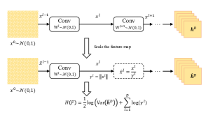
In this subsection, we present the computation of differential entropy for the final feature map generated by a deep network. First, all parameters are initialized by the standard Gaussian distribution . Then we randomly generate an image filled with the standard Gaussian noise and perform forward inference. Based on the discussion in Section 3, the (Gaussian upper bound) entropy of the network is given by
| (3) |
Please note the variance is computed on the last pre-activation feature map .
For deep vanilla networks, directly using Eq. (3) might cause numerical overflow. This is because every layer amplifies the output norm by a large factor. The same issue is also reported in Zen-NAS (Lin et al., 2021). Inspired by the BN rescaling technique proposed in Zen-NAS, we propose an alternative solution without BN layers. We directly re-scale each feature map by some constants during inference, that is , and then compensate the entropy of the network by
| (4) |
The values of can be arbitrarily given, as long as the forward inference does not overflow or underflow. In practice, we find that simply setting to the Euclidean norm of the feature map works well. The process is illustrated in Figure 1. Finally, is multiplied by the size of the feature map as the entropy estimation for this feature map.
Compare with Zen-NAS The principles behind MAE-DET and Zen-NAS are fundamentally different. Zen-NAS uses the gradient norm of the input image as ranking score, and proposes to use two feed-forward inferences to approximate the gradient norm for classification. In contrast, MAE-DET uses an entropy-based score, which only requires one feed-forward inference. Please see the Experiment section for more empirical comparisons.
4.2 Multi-Scale Entropy Prior (MSEP) for Object Detection
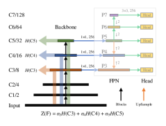
In real-world images, the distribution of object size is not uniform. To bring in this prior knowledge, the detection backbone has 5 stages, where each stage downsamples the feature resolution to half. The MSEP collects the feature map from the last layer of each stage and weighted-sum the corresponding feature map entropies as a new measurement. We name this new measurement multi-scale entropy. The process is illustrated in Figure 2. In this figure, the backbone extracts multi-scale features at different resolutions. Then the FPN neck fuses as input features for the detection head. The multi-scale entropy of backbone is then defined by
| (5) |
where is the entropy of for . The weights store the multi-scale entropy prior to balance the expressivity of different scale features.
How to choose As a concrete example in Fig. 2, the parts of and are generated by up-sampling of , and and are directly generated by down-sampling of (generated by ). Meanwhile, based on the fact that carries sufficient context for detecting objects on various scales (Chen et al., 2021b), is important in the backbone search, so it is good to set a larger value for the weight . Then, different combinations of and correlation analysis are explored in Appendix D, indicating that is good enough for the FPN structure.
4.3 Evolutionary Algorithm for MAE-DET
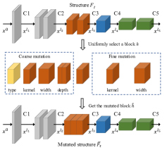
Combining all above, we present our NAS algorithm for MAE-DET in Algorithm 1. The MAE-DET maximizes the multi-scale differential entropy of detection backbones using a customized Evolutionary Algorithm (EA). To improve evolution efficiency, a coarse-to-fine strategy is proposed to reduce the search space gradually. First, we randomly generate seed architectures to fill the population . As shown in Figure 3, a seed architecture consists of a sequence of building blocks, such as ResNet block (He et al., 2016) or MobileNet block (Sandler et al., 2018). Then we randomly select one block and replace it with its mutated version. We use coarse-mutation in the early stages of EA, and switch to fine-mutation after EA iterations. In the coarse-mutation, the block type, kernel size, depth and width are randomly mutated. In the fine-mutation, only kernel size and width are mutated.
After the mutation, if the inference cost of the new structure does not exceed the budget (e.g., FLOPs, parameters and latency) and its depth is smaller than budget , is appended into the population . The maximal depth prevents the algorithm from generating over-deep structures, which will have high entropy with unreasonable structure, and the performance will be worse. During EA iterations, the population is maintained to a certain size by discarding the worst candidate of the smallest multi-scale entropy. At the end of evolution, the backbone with the highest multi-scale entropy is returned.
5 Experiments
In this section, we first describe detail settings for search and training. Then in Subsection 5.2, we apply MAE-DET to design better ResNet-like backbones on COCO dataset (Lin et al., 2014). We align the inference budget with ResNet-50/101. The performance of MAE-DET and ResNet are compared under multiple detection frameworks, including RetinaNet (Lin et al., 2017b), FCOS (Tian et al., 2019), and GFLV2 (Li et al., 2021b). For fairness, we use the same training setting in all experiments for all backbones. In Subsection 5.3, we compare the search cost of MAE-DET to SOTA NAS methods for object detection. Subsection 5.4 reports the ablation studies of different components in MAE-DET. Finally, Subsection 5.5 verifies the transferability of MAE-DET on several detection datasets and segmentation tasks. Due to space limitations, more experiments are postponed to Appendix. Appendix B reports the performance of MAE-DET on mobile devices. Appendix E compare MAE-DET against previous zero-shot NAS methods designed for image classification tasks, showing that these zero-shot NAS methods perform sub-optimally in object detection.
| FLOPs | Params | val2017 | test-dev | FPS | ||||||
| Backbone | Backbone | Backbone | Head | on V100 | ||||||
| ResNet-50 | 83.6G | 23.5M | RetinaNet | 40.2 | 24.3 | 43.3 | 52.2 | - | 23.2 | |
| FCOS | 42.7 | 28.8 | 46.2 | 53.8 | - | 27.6 | ||||
| GFLV2 | 44.7 | 29.1 | 48.1 | 56.6 | 45.1 | 24.2 | ||||
| ResNet-101 | 159.5G | 42.4M | RetinaNet | 42.1 | 25.8 | 45.7 | 54.1 | - | 18.7 | |
| FCOS | 44.4 | 28.3 | 47.9 | 56.9 | - | 21.6 | ||||
| GFLV2 | 46.3 | 29.9 | 50.1 | 58.7 | 46.5 | 19.4 | ||||
| MAE-DET-S | 48.7G | 21.2M | RetinaNet | 40.0 | 23.9 | 43.3 | 52.7 | - | 35.5 | |
| FCOS | 42.5 | 26.8 | 46.0 | 54.6 | - | 43.0 | ||||
| GFLV2 | 44.7 | 27.6 | 48.4 | 58.2 | 44.8 | 37.2 | ||||
| MAE-DET-M | 89.9G | 25.8M | RetinaNet | 42.0 | 26.7 | 45.2 | 55.1 | - | 21.5 | |
| FCOS | 44.5 | 28.6 | 48.1 | 56.1 | - | 24.2 | ||||
| GFLV2 | 46.8 | 29.9 | 50.4 | 60.0 | 46.7 | 22.2 | ||||
| MAE-DET-L | 152.9G | 43.9M | RetinaNet | 43.0 | 27.3 | 46.5 | 56.0 | - | 17.6 | |
| FCOS | 45.9 | 30.2 | 49.4 | 58.4 | - | 19.2 | ||||
| GFLV2 | 47.6 | 30.2 | 51.8 | 60.8 | 48.0 | 18.1 | ||||
5.1 Experiment Settings
Search Settings In MAE-DET, the evolutionary population is set to 256. The total EA iterations . Following the previous designs (Chen et al., 2019b; Jiang et al., 2020; Du et al., 2020), MAE-DET is optimized for FLOPs. The resolution for computing entropy is .
Dataset and Training Details We evaluate detection performance on COCO (Lin et al., 2014) using the official training/testing splits. The mAP is evaluated on val 2017 by default, and GFLV2 is additionally evaluated on test-dev 2007 following common practice. All models are trained from scratch (He et al., 2019) for 6X (73 epochs) on COCO. Following the Spinenet (Du et al., 2020), we use multi-scale training and Synchronized Batch Normalization (SyncBN). For VOC dataset, train-val 2007 and train-val 2012 are used for training, and test 2007 for evaluation. For image classification, all models are trained on ImageNet-1k (Deng et al., 2009) with a batch size of 256 for 120 epochs. Other setting details can be found in Appendix A.
5.2 Design Better ResNet-like Backbones
We search efficient MAE-DET backbones for object detection and align with ResNet-50/101 in Table 1. MAE-DET-S uses 60% less FLOPs than ResNet-50; MAE-DET-M is aligned with ResNet-50 with similar FLOPs and number of parameters as ResNet-50; MAE-DET-L is aligned with ResNet-101. The feature dimension in the FPN and heads is set to 256 for MAE-DET-M and MAE-DET-L but is set to 192 for MAE-DET-S. The fine-tuned results of models pre-trained on ImageNet-1k are reported in Appendix C.
| Method | Training- free | Search Cost GPU Days | Search Part | FLOPs All | Pretrain/ Scratch | Epochs | COCO () |
| DetNAS | backbone | 289G | Pretrain | 24 | 43.4 | ||
| SP-NAS | backbone | 655G | Pretrain | 24 | 47.4 | ||
| SpineNet | 100x TPUv3 | backbone+FPN | 524G | Scratch | 350 | 48.1 | |
| MAE-DET | ✓ | backbone | 279G | Scratch | 73 | 48.0 |
: SpineNet paper did not report the total search cost, only mentioned that 100 TPUv3 was used.
| Backbone | Search Part | Search Space | FLOPs | Params | FPS on V100 | ||||
| DetNAS-3.8G | backbone | ShuffleNetV2 +Xception | 205G | 35.5M | 46.4 | 29.3 | 50.0 | 59.0 | 17.6 |
| SpineNet-96 | backbone+FPN | ResNet Block | 216G | 41.3M | 46.6 | 29.8 | 50.2 | 58.9 | 19.9 |
| MAE-DET-M | backbone | ResNet Block | 215G | 34.9M | 46.8 | 29.9 | 50.4 | 60.0 | 22.2 |
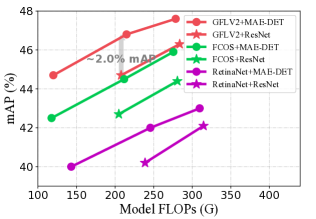
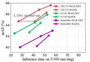
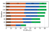
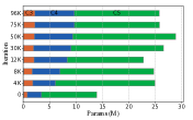
In Table 1, MAE-DET outperforms ResNet by a large margin. The improvements are consistent across three detection frameworks. Particularly, when using the newest framework GFLV2, MAE-DET improves COCO mAP by at the similar FLOPs of ResNet-50, and speeds up the inference by 1.54x times faster at the same accuracy as ResNet-50. Figure 4 visualizes the comparison in Table 1.
Remark Please note that we did not copy the numbers of baseline methods reported in previous works in Table 1 because the mAP depends not only on the architecture, but also on the training schedule, such as training epochs, learning rate, pre-training, etc. Therefore, for a fair comparison, all models in Table 1 are trained by the same training schedule. For comparison with numbers reported in previous works, see Subsection 5.3.
| ImageNet-1K | COCO with YOLOF | COCO with FCOS | ||||||||||
| Score | Mutation | FLOPs | Params | TOP-1 % | ||||||||
| ResNet-50 | None | 4.1G | 23.5M | 78.0 | 37.8 | 19.1 | 42.1 | 53.3 | 38.0 | 23.2 | 40.8 | 47.6 |
| Zen-Score | Coarse | 4.4G | 67.9M | 78.9 | 38.9 | 19.0 | 43.2 | 56.0 | 38.1 | 23.2 | 40.5 | 48.1 |
| Single-scale | Coarse | 4.4G | 60.1M | 78.7 | 39.8 | 19.9 | 44.4 | 56.5 | 38.8 | 23.1 | 41.4 | 50.1 |
| Multi-scale | Coarse | 4.3G | 29.4M | 78.9 | 40.1 | 21.1 | 44.5 | 55.9 | 39.4 | 23.7 | 42.3 | 50.0 |
| Multi-scale | C-to-F | 4.4G | 25.8M | 79.1 | 40.3 | 20.8 | 44.7 | 56.4 | 40.0 | 24.5 | 42.6 | 50.6 |
| Task | Dataset | Head | Backbone | Resolution | Epochs | FLOPs | ||
| Object Detection | VOC | FCOS | ResNet-50 | 12 | 120G | 76.8 | - | |
| MAE-DET-M | 12 | 123G | 80.9 | - | ||||
| Citescapes | ResNet-50 | 64 | 411G | 37.0 | - | |||
| MAE-DET-M | 64 | 426G | 38.1 | - | ||||
| Instance Segmentation | COCO | MASK R-CNN | ResNet-50 | 73 | 375G | 43.2 | 39.2 | |
| MAE-DET-M | 73 | 379G | 44.5 | 40.3 | ||||
| ResNet-50 | 350 | 228G | 42.7 | 37.8 | ||||
| SpineNet-49 | 350 | 216G | 42.9 | 38.1 | ||||
| SCNet | ResNet-50 | 73 | 671G | 46.3 | 41.6 | |||
| MAE-DET-M | 73 | 675G | 47.1 | 42.3 |
: Numbers are cited from SpineNet paper (Du et al., 2020).
5.3 Comparison with SOTA NAS Methods
In Table 2, we compare MAE-DET with SOTA NAS methods for the backbone design in object detection. We directly use the numbers reported in the original papers. Since each NAS method uses different design spaces and training settings, it is impossible to make an absolutely fair comparison for all methods that everyone agrees with. Nevertheless, we list the total search cost, mAP and FLOPs of the best models reported in each work. This gives us an overall impression of how each NAS method works in real-world practice. From Table 2, MAE-DET is the only zero-shot (training-free) method with mAP on COCO, using GPU days of search. SpineNet (Du et al., 2020) achieves a slightly better mAP with 2x more FLOPs. It uses 100 TPUv3 for searching, but the total search cost is not reported in the original paper. MAE-DET achieves better mAP than DetNAS (Chen et al., 2019b) and SP-NAS (Jiang et al., 2020) while being times faster in search.
To further fairly compare different backbones under the same training settings, we train backbones designed by MAE-DET and previous backbone NAS methods in Table 3. Because the implementation of SP-NAS is not open-sourced, we retrain MAE-DET, DetNAS and SpineNet on COCO from scratch. Table 3 shows that MAE-DET requires fewer parameters and has a faster inference speed on V100 when achieving competitive performance over DetNAS and SpineNet on COCO.
5.4 Ablation Study and Analysis
Table 4 reports the MAE-DET backbones searched by different evolutionary strategies, and whether using multi-scale entropy prior. The COCO mAPs of models trained in two detection frameworks (YOLOF and FCOS) are reported in the right big two columns. YOLOF models are trained for 12 epochs with ImageNet pre-trained initialization, while FCOS models are trained with the 3X training epochs. We also compare their image classification ability on ImageNet-1k. All models are constrained by the FLOPs less than 4.4 G while the number of parameters is not constrained. More details about the searching process and architectures can be found in Appendix G, H.
Single-scale entropy Compared to ResNet-50, the model searched by single-scale entropy obtains accuracy gain on ImageNet, mAP gain with FPN-free YOLOF and mAP gain with FPN-based FCOS. Meanwhile, the model searched by Zen-Score achieves accuracy gain on ImageNet, mAP gain with YOLOF and mAP gain with FCOS.
Multi-scale entropy When using multi-scale entropy, both single-scale model and multi-scale model get similar accuracy on ImageNet. The single-scale model uses 2X more parameters than the multi-scale model under the same FLOPs constraint. In terms of mAP, multi-scale model outperforms single-scale model by on COCO with YOLOF and on COCO with FCOS. From the last row of Table 4, the coarse-to-fine mutation further enhances the performance of multi-scale entropy prior, and the overall improvement over ResNet-50 is on ImageNet-1k, on COCO with YOLOF and on COCO with FCOS.
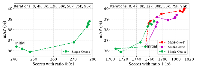
Correlation between entropy and mAP To further study the correlations between model entropy and model mAP, models during the search are trained, and the results are exhibited in Figure 5. The right part of Figure 5 indicates that the mAP positively correlates with the multi-scale entropy. The left part of Figure 5 reveals that the single-scale entropy cannot represent the mAP well, so multi-scale entropy is necessary for detection tasks. By analyzing the structures in Appendix G, the computation of single-scale models is concentrated in the last stage , ignoring the and stages, and leading to the worse multi-scale score. Instead, multi-scale models allocate more computation to the previous stages to enhance the expressivity of and , which improve the multi-scale score.
Discussion about dataset We agree that the dataset is powerful for ranking the architectures in the training-based methods. However, the process of MAE-DET search is performed without data training. If we replace the Gaussian input directly with target data, the output after one convolution is also random due to the Gaussian initialized weights. On the other hand, the FPN framework has considered data distribution characteristics according to previous works (Lin et al., 2017a; Tian et al., 2019; Li et al., 2021b). Thus, the aim of MAE-Det is to provide a better multi-scale feature extractor under the given inference budgets. We believe the zero-shot method combined with target data without training can be a future research direction.
5.5 Transfer to Other Tasks
VOC and Cityscapes To evaluate the transferability of MAE-DET in different datasets, we transfer the FCOS-based MAE-DET-M to VOC and Cityscapes dataset, as shown in the upper half of Table 5. The models are fine-tuned after being pre-trained on ImageNet. Comparing to ResNet-50, MAE-DET-M achieves better mAP in VOC, better mAP in Cityscape.
Instance Segmentation The lower half of Table 5 reports results of Mask R-CNN (He et al., 2017) and SCNet (Vu et al., 2021) models for the COCO instance segmentation task with 6X training from scratch. Comparing to ResNet-50, MAE-DET-M achieves better AP and mask AP with similar model size and FLOPs on Mask RCNN and SCNet.
6 Conclusion
In this paper, we revisit the Maximum Entropy Principle in zero-shot NAS for object detection. The proposed MAE-DET achieves competitive detection accuracy with search speed orders of magnitude faster than previous training-based NAS methods. While modern object detection backbones involve more complex building blocks and network topologies, the design of MAE-DET is conceptually simple and easy to implement, demonstrating the grace of “simple is better” philosophy. Extensive experiments and analyses on various datasets validate its excellent transferability.
References
- Abadi et al. (2015) Abadi, M., Agarwal, A., Barham, P., Brevdo, E., Chen, Z., Citro, C., Corrado, G. S., Davis, A., Dean, J., Devin, M., Ghemawat, S., Goodfellow, I., Harp, A., Irving, G., Isard, M., Jia, Y., Jozefowicz, R., Kaiser, L., Kudlur, M., Levenberg, J., Mané, D., Monga, R., Moore, S., Murray, D., Olah, C., Schuster, M., Shlens, J., Steiner, B., Sutskever, I., Talwar, K., Tucker, P., Vanhoucke, V., Vasudevan, V., Viégas, F., Vinyals, O., Warden, P., Wattenberg, M., Wicke, M., Yu, Y., and Zheng, X. TensorFlow: Large-scale machine learning on heterogeneous systems, 2015. URL https://www.tensorflow.org/.
- Brillouin (2013) Brillouin, L. Science and information theory. Courier Corporation, 2013.
- Cai et al. (2019) Cai, H., Gan, C., Wang, T., Zhang, Z., and Han, S. Once-for-all: Train one network and specialize it for efficient deployment. arXiv preprint arXiv:1908.09791, 2019.
- Chan et al. (2021) Chan, K. H. R., Yu, Y., You, C., Qi, H., Wright, J., and Ma, Y. ReduNet: A White-box Deep Network from the Principle of Maximizing Rate Reduction. arXiv:2105.10446, 2021.
- Chen et al. (2019a) Chen, K., Wang, J., Pang, J., Cao, Y., Xiong, Y., Li, X., Sun, S., Feng, W., Liu, Z., Xu, J., Zhang, Z., Cheng, D., Zhu, C., Cheng, T., Zhao, Q., Li, B., Lu, X., Zhu, R., Wu, Y., Dai, J., Wang, J., Shi, J., Ouyang, W., Loy, C. C., and Lin, D. MMDetection: Open mmlab detection toolbox and benchmark. arXiv preprint arXiv:1906.07155, 2019a.
- Chen et al. (2021a) Chen, M., Peng, H., Fu, J., and Ling, H. Autoformer: Searching transformers for visual recognition. In Proceedings of the IEEE/CVF International Conference on Computer Vision, pp. 12270–12280, 2021a.
- Chen et al. (2021b) Chen, Q., Wang, Y., Yang, T., Zhang, X., Cheng, J., and Sun, J. You only look one-level feature. In Proceedings of the IEEE/CVF Conference on Computer Vision and Pattern Recognition, pp. 13039–13048, 2021b.
- Chen et al. (2021c) Chen, W., Gong, X., and Wang, Z. Neural architecture search on imagenet in four gpu hours: A theoretically inspired perspective. In Proceedings of the International Conference on Learning Representations, 2021c.
- Chen et al. (2019b) Chen, Y., Yang, T., Zhang, X., Meng, G., Xiao, X., and Sun, J. Detnas: Backbone search for object detection. Advances in Neural Information Processing Systems, 32:6642–6652, 2019b.
- Chu et al. (2021) Chu, X., Wang, X., Zhang, B., Lu, S., Wei, X., and Yan, J. Darts-: Robustly stepping out of performance collapse without indicators. In International Conference on Learning Representations, 2021.
- Cover & Thomas (2012) Cover, T. M. and Thomas, J. A. Elements of Information Theory. John Wiley & Sons, 2012.
- Deng et al. (2009) Deng, J., Dong, W., Socher, R., Li, L.-J., Li, K., and Fei-Fei, L. Imagenet: A large-scale hierarchical image database. In 2009 IEEE conference on computer vision and pattern recognition, pp. 248–255. Ieee, 2009.
- Du et al. (2020) Du, X., Lin, T.-Y., Jin, P., Ghiasi, G., Tan, M., Cui, Y., Le, Q. V., and Song, X. Spinenet: Learning scale-permuted backbone for recognition and localization. In Proceedings of the IEEE/CVF conference on computer vision and pattern recognition, pp. 11592–11601, 2020.
- Fang et al. (2020) Fang, J., Sun, Y., Zhang, Q., Peng, K., Li, Y., Liu, W., and Wang, X. Fna++: Fast network adaptation via parameter remapping and architecture search. IEEE Transactions on Pattern Analysis and Machine Intelligence, 43(9):2990–3004, 2020.
- Ghiasi et al. (2019) Ghiasi, G., Lin, T.-Y., and Le, Q. V. Nas-fpn: Learning scalable feature pyramid architecture for object detection. In Proceedings of the IEEE/CVF Conference on Computer Vision and Pattern Recognition, pp. 7036–7045, 2019.
- Hanin & Rolnick (2019) Hanin, B. and Rolnick, D. Complexity of linear regions in deep networks. In International Conference on Machine Learning, pp. 2596–2604. PMLR, 2019.
- He et al. (2016) He, K., Zhang, X., Ren, S., and Sun, J. Deep residual learning for image recognition. In Proceedings of the IEEE conference on computer vision and pattern recognition, pp. 770–778, 2016.
- He et al. (2017) He, K., Gkioxari, G., Dollár, P., and Girshick, R. Mask r-cnn. In Proceedings of the IEEE international conference on computer vision, pp. 2961–2969, 2017.
- He et al. (2019) He, K., Girshick, R., and Dollár, P. Rethinking imagenet pre-training. In Proceedings of the IEEE/CVF International Conference on Computer Vision, pp. 4918–4927, 2019.
- Hu et al. (2018) Hu, J., Shen, L., and Sun, G. Squeeze-and-excitation networks. In Proceedings of the IEEE conference on computer vision and pattern recognition, pp. 7132–7141, 2018.
- Ioffe & Szegedy (2015) Ioffe, S. and Szegedy, C. Batch normalization: Accelerating deep network training by reducing internal covariate shift. In International conference on machine learning, pp. 448–456. PMLR, 2015.
- Jaynes (1957) Jaynes, E. T. Information theory and statistical mechanics. Phys. Rev., 106(4):620–630, May 1957.
- Jiang et al. (2020) Jiang, C., Xu, H., Zhang, W., Liang, X., and Li, Z. Sp-nas: Serial-to-parallel backbone search for object detection. In Proceedings of the IEEE/CVF Conference on Computer Vision and Pattern Recognition, pp. 11863–11872, 2020.
- Jiang et al. (2022) Jiang, Y., Tan, Z., Wang, J., Sun, X., Lin, M., and Li, H. Giraffedet: A heavy-neck paradigm for object detection. In International Conference on Learning Representations, 2022.
- Kullback (1997) Kullback, S. Information theory and statistics. Courier Corporation, 1997.
- Li et al. (2021a) Li, C., Wang, G., Wang, B., Liang, X., Li, Z., and Chang, X. Ds-net++: Dynamic weight slicing for efficient inference in cnns and transformers. arXiv preprint arXiv:2109.10060, 2021a.
- Li et al. (2020) Li, X., Wang, W., Wu, L., Chen, S., Hu, X., Li, J., Tang, J., and Yang, J. Generalized focal loss: Learning qualified and distributed bounding boxes for dense object detection. In NeurIPS, 2020.
- Li et al. (2021b) Li, X., Wang, W., Hu, X., Li, J., Tang, J., and Yang, J. Generalized focal loss v2: Learning reliable localization quality estimation for dense object detection. In Proceedings of the IEEE/CVF Conference on Computer Vision and Pattern Recognition, pp. 11632–11641, 2021b.
- Li et al. (2018) Li, Z., Peng, C., Yu, G., Zhang, X., Deng, Y., and Sun, J. Detnet: Design backbone for object detection. In Proceedings of the European conference on computer vision, pp. 334–350, 2018.
- Liang et al. (2021) Liang, T., Wang, Y., Tang, Z., Hu, G., and Ling, H. Opanas: One-shot path aggregation network architecture search for object detection. In Proceedings of the IEEE/CVF Conference on Computer Vision and Pattern Recognition, pp. 10195–10203, 2021.
- Lin et al. (2020) Lin, J., Chen, W.-M., Cohn, J., Gan, C., and Han, S. Mcunet: Tiny deep learning on iot devices. In Annual Conference on Neural Information Processing Systems (NeurIPS), 2020.
- Lin et al. (2021) Lin, M., Wang, P., Sun, Z., Chen, H., Sun, X., Qian, Q., Li, H., and Jin, R. Zen-nas: A zero-shot nas for high-performance deep image recognition. In 2021 IEEE/CVF International Conference on Computer Vision, 2021.
- Lin et al. (2014) Lin, T.-Y., Maire, M., Belongie, S., Hays, J., Perona, P., Ramanan, D., Dollár, P., and Zitnick, C. L. Microsoft coco: Common objects in context. In European conference on computer vision, pp. 740–755. Springer, 2014.
- Lin et al. (2017a) Lin, T.-Y., Dollár, P., Girshick, R., He, K., Hariharan, B., and Belongie, S. Feature pyramid networks for object detection. In Proceedings of the IEEE conference on computer vision and pattern recognition, pp. 2117–2125, 2017a.
- Lin et al. (2017b) Lin, T.-Y., Goyal, P., Girshick, R., He, K., and Dollár, P. Focal loss for dense object detection. In Proceedings of the IEEE international conference on computer vision, pp. 2980–2988, 2017b.
- Liu et al. (2018) Liu, H., Simonyan, K., and Yang, Y. Darts: Differentiable architecture search. arXiv preprint arXiv:1806.09055, 2018.
- Loshchilov & Hutter (2017) Loshchilov, I. and Hutter, F. Sgdr: Stochastic gradient descent with warm restarts. In Proceedings of the International Conference on Learning Representations, 2017.
- Mellor et al. (2021) Mellor, J., Turner, J., Storkey, A., and Crowley, E. J. Neural architecture search without training. In International Conference on Machine Learning, pp. 7588–7598. PMLR, 2021.
- Newell et al. (2016) Newell, A., Yang, K., and Deng, J. Stacked hourglass networks for human pose estimation. In European conference on computer vision, pp. 483–499. Springer, 2016.
- Norwich (1993) Norwich, K. H. Information, sensation, and perception. Academic Press San Diego, pp. 81-82, 1993.
- Paszke et al. (2019) Paszke, A., Gross, S., Massa, F., Lerer, A., Bradbury, J., Chanan, G., Killeen, T., Lin, Z., Gimelshein, N., Antiga, L., Desmaison, A., Kopf, A., Yang, E., DeVito, Z., Raison, M., Tejani, A., Chilamkurthy, S., Steiner, B., Fang, L., Bai, J., and Chintala, S. Pytorch: An imperative style, high-performance deep learning library. In Wallach, H., Larochelle, H., Beygelzimer, A., d'Alché-Buc, F., Fox, E., and Garnett, R. (eds.), Advances in Neural Information Processing Systems 32, pp. 8024–8035. Curran Associates, Inc., 2019.
- Peng et al. (2019) Peng, J., Sun, M., ZHANG, Z.-X., Tan, T., and Yan, J. Efficient neural architecture transformation search in channel-level for object detection. Advances in Neural Information Processing Systems, 32, 2019.
- Poole et al. (2016) Poole, B., Lahiri, S., Raghu, M., Sohl-Dickstein, J., and Ganguli, S. Exponential expressivity in deep neural networks through transient chaos. Advances in neural information processing systems, 29:3360–3368, 2016.
- Real et al. (2019) Real, E., Aggarwal, A., Huang, Y., and Le, Q. V. Regularized evolution for image classifier architecture search. In Proceedings of the aaai conference on artificial intelligence, volume 33, pp. 4780–4789, 2019.
- Reza (1994) Reza, F. M. An introduction to information theory. Courier Corporation, 1994.
- Sandler et al. (2018) Sandler, M., Howard, A., Zhu, M., Zhmoginov, A., and Chen, L.-C. Mobilenetv2: Inverted residuals and linear bottlenecks. In Proceedings of the IEEE conference on computer vision and pattern recognition, pp. 4510–4520, 2018.
- Saxe et al. (2018) Saxe, A. M., Bansal, Y., Dapello, J., Advani, M., Kolchinsky, A., Tracey, B. D., and Cox, D. D. On the information bottleneck theory of deep learning. In ICLR, 2018.
- Serra et al. (2018) Serra, T., Tjandraatmadja, C., and Ramalingam, S. Bounding and counting linear regions of deep neural networks. In International Conference on Machine Learning, pp. 4558–4566. PMLR, 2018.
- Shannon (1948) Shannon, C. E. A mathematical theory of communication. The Bell system technical journal, 27(3):379–423, 1948.
- Sun et al. (2018) Sun, S., Pang, J., Shi, J., Yi, S., and Ouyang, W. Fishnet: A versatile backbone for image, region, and pixel level prediction. In Advances in Neural Information Processing Systems, pp. 760–770, 2018.
- Tan & Le (2019) Tan, M. and Le, Q. Efficientnet: Rethinking model scaling for convolutional neural networks. In International Conference on Machine Learning, pp. 6105–6114. PMLR, 2019.
- Tan et al. (2020) Tan, M., Pang, R., and Le, Q. V. Efficientdet: Scalable and efficient object detection. In Proceedings of the IEEE/CVF conference on computer vision and pattern recognition, pp. 10781–10790, 2020.
- Tanaka et al. (2020) Tanaka, H., Kunin, D., Yamins, D. L., and Ganguli, S. Pruning neural networks without any data by iteratively conserving synaptic flow. In Proceedings of the International Conference on Neural Information Processing Systems, 2020.
- Tian et al. (2019) Tian, Z., Shen, C., Chen, H., and He, T. Fcos: Fully convolutional one-stage object detection. In Proceedings of the IEEE/CVF international conference on computer vision, pp. 9627–9636, 2019.
- Vu et al. (2021) Vu, T., Kang, H., and Yoo, C. D. Scnet: Training inference sample consistency for instance segmentation. In Proceedings of the AAAI Conference on Artificial Intelligence, volume 35, pp. 2701–2709, 2021.
- Wang et al. (2020a) Wang, J., Sun, K., Cheng, T., Jiang, B., Deng, C., Zhao, Y., Liu, D., Mu, Y., Tan, M., Wang, X., et al. Deep high-resolution representation learning for visual recognition. IEEE transactions on pattern analysis and machine intelligence, 2020a.
- Wang et al. (2020b) Wang, N., Gao, Y., Chen, H., Wang, P., Tian, Z., Shen, C., and Zhang, Y. Nas-fcos: Fast neural architecture search for object detection. In Proceedings of the IEEE/CVF Conference on Computer Vision and Pattern Recognition, pp. 11943–11951, 2020b.
- Xie et al. (2017) Xie, S., Girshick, R., Dollár, P., Tu, Z., and He, K. Aggregated residual transformations for deep neural networks. In Proceedings of the IEEE conference on computer vision and pattern recognition, pp. 1492–1500, 2017.
- Xiong et al. (2021) Xiong, Y., Liu, H., Gupta, S., Akin, B., Bender, G., Wang, Y., Kindermans, P.-J., Tan, M., Singh, V., and Chen, B. Mobiledets: Searching for object detection architectures for mobile accelerators. In Proceedings of the IEEE/CVF Conference on Computer Vision and Pattern Recognition, pp. 3825–3834, 2021.
- Yu et al. (2020) Yu, Y., Chan, K. H. R., You, C., Song, C., and Ma, Y. Learning diverse and discriminative representations via the principle of maximal coding rate reduction. Advances in Neural Information Processing Systems, 33:9422–9434, 2020.
- Zhao et al. (2020) Zhao, H., Jia, J., and Koltun, V. Exploring self-attention for image recognition. In Proceedings of the IEEE/CVF Conference on Computer Vision and Pattern Recognition, pp. 10076–10085, 2020.
- Zhu et al. (2019) Zhu, X., Hu, H., Lin, S., and Dai, J. Deformable convnets v2: More deformable, better results. In Proceedings of the IEEE/CVF Conference on Computer Vision and Pattern Recognition, pp. 9308–9316, 2019.
- Zoph et al. (2018) Zoph, B., Vasudevan, V., Shlens, J., and Le, Q. V. Learning transferable architectures for scalable image recognition. In Proceedings of the IEEE conference on computer vision and pattern recognition, pp. 8697–8710, 2018.
Appendix A Training Details
Searching Details In MAE-DET, the evolutionary population is set as 256 while total iterations . Residual blocks and bottleneck blocks are utilized as searching space when comparing with ResNet series backbone (He et al., 2016). Following the previous designs (Chen et al., 2019b; Jiang et al., 2020; Du et al., 2020), MAE-DET is optimized for the budget of FLOPs according to the target networks, i.e., ResNet-50 and ResNet-101. To balance the computational complexity and large resolution demand, the resolution in search is set as for MAE-DET. When starting the search, the initial structure is composed of 5 downsampling stages with small and narrow blocks to meet the reasoning budget. In the mutation, whether the coarse-mutation or fine-mutation, the width of the selected block is mutated in a given scale , while the depth increases or decreases 1 or 2. The kernel size is searched in set . Note that blocks deeper than 10 will be divided into two blocks equally to enhance diversity.
Dataset and Training Details For object detection, trainval35k with 115K images in the COCO dataset is mainly used for training. With the single-scale testing of resolution , COCO mAP results are reported on the val 2017 for most experiments and the test-dev 2007 for GFLV2 results in Table 1. When training on the COCO dataset, the initial learning rate is set to , and decays two times with the ratio of during training. SGD is adopted as optimizer with momentum 0.9; weight decay of ; batch size of 16 (on 8 Nvidia V100 GPUs); patch size of .
Additionally, multi-scale training and Synchronized Batch Normalization (SyncBN) are adopted to enhance the stability of the scratch training without increasing the complexity of inference. Training from scratch is used to avoid the gap between ImageNet pre-trained models, to ensure a fair comparison with baselines. 3X learning schedule is applied for the ablation study with a multi-scale range between (36 epochs, decays at 28 and 33 epochs), and 6X learning schedule for the SOTA comparisons with the range between (73 epochs, decays at 65 and 71 epochs). All object detection training is produced under mmdetection (Chen et al., 2019a) for fair comparisons, and hyper-parameters not mentioned in the paper are always set to default values in mmdection.
For image classification, all models are trained on ImageNet-1K with a batch size of 256 for 120 epochs. When training on ImageNet-1K, we use SGD optimizer with momentum 0.9; cosine learning rate decay (Loshchilov & Hutter, 2017); initial learning rate 0.1; weight decay .
Appendix B MAE-DET for Mobile Device
| FLOPs | Params | val2017 | FPS | ||||
| Backbone | Backbone | Backbone | on Pixel 2 | ||||
| MobileNetV2-0.5 | 217M | 0.7M | 14.7 | 0.8 | 11.0 | 31.2 | 13.5 |
| MobileNetV2-1.0 | 651M | 2.2M | 21.1 | 1.7 | 20.5 | 39.9 | 6.6 |
| MAE-DET-MB-S | 201M | 0.6M | 15.9 | 0.8 | 12.2 | 31.8 | 13.8 |
| MAE-DET-MB-M | 645M | 2.0M | 22.2 | 2.1 | 21.5 | 42.3 | 6.3 |
| MAE-DET-MB-M-SE | 647M | 2.3M | 22.6 | 2.3 | 22.0 | 42.5 | 5.6 |
For mobile-size object detection, we explore building MAE-DET-MB with MobileNetV2 (Sandler et al., 2018) blocks, using the inverted bottleneck block with expansion ratio of 1/3/6. The weight ratio is still set as 1:1:6, and other searching settings are the same as the Resnet-like searching. In Table. 6, MAE-DET-MB use less computation and parameters, but outperform MobileNetV2 by 1% AP with similar inference time on Google Pixel 2 phone. Additionally, inserting SE modules to MAE-DET-MB-M can improve the mAP by 0.4%.
Appendix C Object Detection with ImageNet Pre-train Models
In the main body of the paper, training from scratch is used to avoid the gap between ImageNet pre-trained models, to ensure a fair comparison with baselines (He et al., 2019). Since 6X training from scratch consumes 3 times more time than 2X pre-trained training, we use the ImageNet pre-trained model to initialize the MAE-DET-M in various heads, including RetinaNet, FCOS and GFLV2. As present in Table. 1, 7, whether using training from scratch or ImageNet pre-training, MAE-DET can outperform ResNet-50 in the three popular FPN-based frameworks by large margins.
| Backbone | FLOPs Backbone | Params Backbone | Head | Strategy | Epochs | ||||
| ResNet-50 | 83.6G | 23.5M | GFLV2 | Scratch | 73 | 44.7 | 29.1 | 48.1 | 56.6 |
| GFLV2 | Pretrain | 24 | 44.0 | 27.1 | 47.8 | 56.1 | |||
| GFLV2 | Pretrain | 24 | 43.9 | - | - | - | |||
| MAE-DET-M | 89.9G | 25.8M | RetinaNet | Scratch | 73 | 42.0 | 26.7 | 45.2 | 55.1 |
| RetinaNet | Pretrain | 24 | 42.3 | 25.3 | 46.5 | 56.0 | |||
| FCOS | Scratch | 73 | 44.5 | 28.6 | 48.1 | 56.1 | |||
| FCOS | Pretrain | 24 | 44.5 | 28.8 | 48.5 | 56.9 | |||
| GFLV2 | Scratch | 73 | 46.8 | 29.9 | 50.4 | 60.0 | |||
| GFLV2 | Pretrain | 24 | 46.0 | 29.0 | 50.0 | 59.9 |
: results in this line are reported in the official github (Li et al., 2021b).
Appendix D Multi-scale Entropy Prior Ablation Study
| Backbone | :: | FLOPs | Params | |||||||
| ResNet-50 | None | 83.6G | 23.5M | 38.0 | 55.2 | 41.0 | 23.2 | 40.8 | 47.6 | |
| MAE-DET | 1:1:1 | 84.4G | 11.5M | 37.4 | 54.6 | 40.0 | 23.6 | 39.8 | 46.6 | |
| MAE-DET | 1:1:2 | 84.8G | 13.4M | 37.8 | 54.9 | 40.5 | 23.2 | 40.0 | 47.8 | |
| MAE-DET | 1:1:4 | 85.9G | 17.2M | 38.6 | 56.0 | 41.4 | 23.4 | 41.3 | 48.6 | |
| MAE-DET | 1:1:6 | 88.7G | 29.4M | 39.4 | 57.3 | 42.1 | 23.7 | 42.3 | 50.0 | |
| MAE-DET | 1:1:8 | 89.9G | 31.7M | 39.4 | 57.2 | 42.0 | 23.7 | 42.5 | 49.5 | |
| MAE-DET | 1:4:1 | 86.3G | 10.9M | 35.7 | 52.6 | 38.3 | 22.2 | 38.1 | 44.9 | |
| MAE-DET | 4:1:1 | 86.1G | 11.1M | 33.9 | 50.2 | 36.7 | 20.4 | 36.1 | 43.4 |
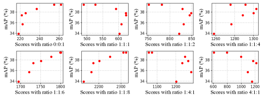
In Table 8, we tune the different arrangements of multi-scale weights in a wide range. Seven multi-scale weight ratios are used to search different models, and all models are trained on the COCO dataset with FCOS and 3X learning schedule. Table 8 shows that if the same weights are arranged to -, the performance of MAE-DET on COCO is worse than ResNet-50. Considering the importance of (discussed in Section 4.2), we increase the weight of , and MAE-DET’s performance continues to improve. To further explore the correlations between mAP and scores, we use the seven weight ratios to calculate the different scores of each model, along with the single-scale weight ratio of 0:0:1. The correlations between mAP and different scores are plotted in Figure 6. Taking the results in Table 8 and Figure 6, we confirm the ratio of 1:1:6 may be good enough for the current FPN structure.
Appendix E Comparison with Zero-Shot Proxies for Image Classification
| Proxy | FLOPs Backbone | Params Backbone | ||||
| ResNet-50 | 84G | 23.5M | 38.0 | 23.2 | 40.8 | 47.6 |
| SyncFlow | 90G | 67.4M | 35.6 | 21.8 | 38.1 | 44.8 |
| NASWOT | 88G | 28.1M | 36.7 | 23.1 | 38.8 | 45.9 |
| Zen-NAS | 91G | 67.9M | 38.1 | 23.2 | 40.5 | 48.1 |
| MAE-DET | 89G | 25.8M | 39.4 | 23.7 | 42.3 | 50.0 |
We compare MAE-DET with architectures designed by zero-shot proxies for image classification in previous works, including SyncFlow (Tanaka et al., 2020), NASWOT (Mellor et al., 2021), ZenNAS (Lin et al., 2021). For a fair comparison, all methods use the same search space, FLOPs budget , searching strategy and training schedule. All searched backbones are trained on COCO with the FCOS head and 3X training from scratch. The results are reported in Table. 9.
Among these methods, SyncFlow and NASWOT perform worse than ResNet-50 on COCO albeit they show competitive performance in image classification tasks. Zen-NAS achieves competitive performance over ResNet-50. The MAE-DET outperforms Zen-NAS by mAP with slightly fewer FLOPs and nearly one third of parameters.
Appendix F Random search comparisons
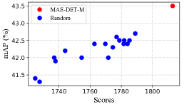
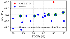
Using the same search space as MAE-DET-M, we randomly sample models within 70-95G FLOPs and 20-30M parameters without MAE score. Due to the high cost of sampling, 17 random models are currently sampled and trained on GFLV2 with a 3X learning schedule. The correlations are shown in Fig. 7. Our MAE-DET model has better performance than the random searched models.
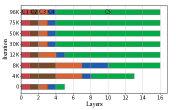
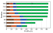
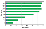
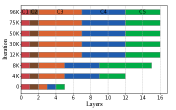
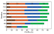
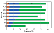
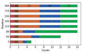
Appendix G Visualization of Search process
Appendix H Detail Structure of MAE-DETs
The ’block’ column is the block type. ’Conv’ is the standard convolution layer followed by BN and RELU. ’ResBlock’ is the residual bottleneck block used in ResNet-50 and is stacked by two Blocks in our design. ’kernel’ is the kernel size of kxk convolution layer in each block. ’in’, ’out’ and ’bottleneck’ are numbers of input channels, output channels and bottleneck channels respectively. ’stride’ is the stride of current block. ’# layers’ is the number of duplication of current block type.
| block | kernel | in | out | stride | bottleneck | # layers | level |
| Conv | 3 | 3 | 96 | 2 | - | 1 | C1 |
| ResBlock | 5 | 96 | 208 | 2 | 32 | 2 | C2 |
| ResBlock | 5 | 208 | 560 | 2 | 56 | 1 | C3 |
| ResBlock | 5 | 560 | 1264 | 2 | 112 | 2 | C4 |
| ResBlock | 5 | 1264 | 1712 | 2 | 224 | 3 | C5 |
| ResBlock | 5 | 1712 | 2048 | 1 | 224 | 3 | C5 |
| ResBlock | 5 | 2048 | 2048 | 1 | 256 | 4 | C5 |
| block | kernel | in | out | stride | bottleneck | # layers | level |
| Conv | 3 | 3 | 32 | 2 | - | 1 | C1 |
| ResBlock | 5 | 32 | 128 | 2 | 24 | 1 | C2 |
| ResBlock | 5 | 128 | 512 | 2 | 72 | 5 | C3 |
| ResBlock | 5 | 512 | 1632 | 2 | 112 | 5 | C4 |
| ResBlock | 5 | 1632 | 2048 | 2 | 216 | 4 | C5 |
| block | kernel | in | out | stride | bottleneck | # layers | level |
| Conv | 3 | 3 | 64 | 2 | - | 1 | C1 |
| ResBlock | 3 | 64 | 120 | 2 | 64 | 1 | C2 |
| ResBlock | 5 | 120 | 512 | 2 | 72 | 5 | C3 |
| ResBlock | 5 | 512 | 1632 | 2 | 112 | 5 | C4 |
| ResBlock | 5 | 1632 | 2048 | 2 | 184 | 4 | C5 |
| block | kernel | in | out | stride | bottleneck | # layers | level |
| Conv | 3 | 3 | 32 | 2 | - | 1 | C1 |
| ResBlock | 5 | 32 | 48 | 2 | 32 | 1 | C2 |
| ResBlock | 3 | 48 | 272 | 2 | 120 | 2 | C3 |
| ResBlock | 5 | 272 | 1024 | 2 | 80 | 5 | C4 |
| ResBlock | 3 | 1024 | 2048 | 2 | 240 | 5 | C5 |
| block | kernel | in | out | stride | bottleneck | # layers | level |
| Conv | 3 | 3 | 80 | 2 | - | 1 | C1 |
| ResBlock | 3 | 80 | 144 | 2 | 80 | 1 | C2 |
| ResBlock | 5 | 144 | 608 | 2 | 88 | 6 | C3 |
| ResBlock | 5 | 608 | 1912 | 2 | 136 | 6 | C4 |
| ResBlock | 5 | 1912 | 2400 | 2 | 220 | 5 | C5 |
| block | kernel | in | out | stride | bottleneck | # layers | level |
| Conv | 3 | 3 | 64 | 2 | - | 1 | C1 |
| ResBlock | 3 | 64 | 256 | 2 | 64 | 1 | C2 |
| ResBlock | 3 | 256 | 512 | 2 | 128 | 1 | C3 |
| ResBlock | 3 | 512 | 1024 | 2 | 256 | 1 | C4 |
| ResBlock | 3 | 1024 | 2048 | 2 | 512 | 1 | C5 |