A Kernel Test for Causal Association via
Noise Contrastive Backdoor Adjustment

Abstract

Causal inference grows increasingly complex as the number of confounders increases. Given treatments $X$, confounders $Z$ and outcomes $Y$, we develop a non-parametric method to test the do-null hypothesis $H_{0}:\;p(y|\text{\it do}(X=x))=p(y)$ against the general alternative. Building on the Hilbert Schmidt Independence Criterion (HSIC) for marginal independence testing, we propose backdoor-HSIC (bd-HSIC) and demonstrate that it is calibrated and has power for both binary and continuous treatments under a large number of confounders. Additionally, we establish convergence properties of the estimators of covariance operators used in bd-HSIC. We investigate the advantages and disadvantages of bd-HSIC against parametric tests as well as the importance of using the do-null testing in contrast to marginal independence testing or conditional independence testing. A complete implementation can be found at https://github.com/MrHuff/kgformula.

Keywords: Causal Inference, Noise Contrastive Estimation, Kernel Methods, Backdoor Adjustment, HSIC

1 Introduction and Related Work

Modern causal inference often considers very large datasets with many confounders that may have vastly different properties. These settings are considered in a wide range of applications where randomized controlled trials are not always readily available: epidemiology (Rothman and Greenland, 2005), brain imaging (Castro et al., 2020), retail (Moriyama and Kuwano, 2021), entertainment platforms (Dawen Liang and Blei, 2020). The inference setting is often complex, with high dimensional confounding variables needing to be accounted for. In such complex settings, non-parametric inference schemes that answer a simple causal query of causal association are needed as an initial step before more sophisticated causal relationships can be established.

G-computation (Robins, 1986) is a classical method for estimating a causal effect from observational studies involving variables that are both mediators and confounders. The popularity of g-computation persists to this day (Daniel et al., 2013; Keil et al., 2020), because it allows one to test for a non-null causal effect using a variety of postulated models fulfilling the so-called backdoor criterion. However, the use of parametric models in this context can lead to a problem known as the g-null paradox (Robins and Wasserman, 1997), in which the null being tested cannot logically hold because the models specified are insufficiently flexible (McGrath et al., 2021).

In this paper, we propose a non-parametric approach for the test of the absence of causal effect. In the Reproducing Kernel Hilbert Space (RKHS) and machine learning literature, the Hilbert-Schmidt Independence Criterion (HSIC) introduced by Gretton et al. (2005) is a widely used approach to non-parametric testing of independence. As the HSIC has good power properties and it is applicable to multivariate settings as well as to random variables taking values in generic domains, we use it as a foundation in this paper. Using G-computation principles, we introduce an extension of HSIC that can be applied to causal association testing. We compare against the popular post-double selection (PDS) method (Belloni et al., 2014), a parametric lasso-based model that is widely used for causal estimation.

We summarize our contributions as follows:

1. We introduce bd-HSIC, which is derived analogously to HSIC but instead uses importance weighted covariance operators, and further establish the convergence properties of the corresponding estimators in the causal setting.

2. We demonstrate that bd-HSIC is calibrated and has good power for different types of treatments and a large number of confounders when testing the do-null.

3. We analyze bd-HSIC by providing ablation studies and characterize under which circumstances bd-HSIC becomes invalid.

The rest of the paper is organized as follows: Section 2 describes the problem setting and provides a background on HSIC, Section 3 presents bd-HSIC and establishes convergence properties of the associated estimators, Section 4 presents additional details on the estimation procedure of bd-HSIC, Section 5 provides the experimental results and we conclude the paper in Section 6.

2 Background

Consider a situation where we observe treatments $X$, outcomes $Y$ and confounders $Z$ defined on measurable spaces $\mathcal{X}$, $\mathcal{Y}$, and $\mathcal{Z}$, respectively. We assume these quantities are observed as $\left\{(x_{i},y_{i},z_{i})\right\}_{i=1}^{n}\sim p$, where $p$ is some joint probability density on the product space $\mathcal{X}\times\mathcal{Y}\times\mathcal{Z}$. We are interested in establishing a causal relationship between treatments $X$ and outcomes $Y$. In ideal circumstances, we would not have any confounders and such a relationship can be established straightforwardly, using e.g. regression methods. However, such circumstances are extremely rare and would require that the treatment is assigned to units at random. In the more common case of observational studies, dependencies between $X,Y,Z$ are often depicted as in Figure 1. The existence of confounders $Z$ complicates establishing the causal relationship between $X$ and $Y$, as they introduce dependence between $X$ and $Y$ which is difficult to disentangle from the postulated causal effect.

Figure 1: The relationship between treatments $X$, outcomes $Y$, and confounders $Z$

do-null Independence Testing.

Let

$$p(y|\text{do}(x)):=\int p(y|x,z)p(z)dz$$

where in general $p(y|x)\neq p(y|\text{do}(x))$ since $X$ and $Z$ may be dependent. We are interested in testing the hypothesis

$$H_{0}:p(y|\text{\it do}(x))=p(y)$$ (1)

versus the general alternative.

A motivating real world problem

In development economics, it is of great importance to establish causes to infant mortality (Ensor et al., 2010). The causes may often have a non-linear association with the mortality while being confounded by circumstantial factors such as the socio-economical background of the parents and the medical history of the mother. We will illustrate throughout the paper the importance of a non-parametric test that is able to capture non-linear dependencies for different treatments under a large number of confounders.

In this paper, we will introduce a test statistic for the hypothesis (1), but first we review HSIC (Gretton et al., 2005), which serves as the foundation for our contribution.

2.1 Hilbert-Schmidt Independence Criterion

The Hilbert-Schmidt Independence Criterion (HSIC) is a powerful non-parametric test of independence for high dimensional data. It considers the problem of empirically establishing whether there is any form of departure from independence between two random variables taking values on generic domains.

Marginal Independence Testing.

Let $P_{xy}$ be a Borel probability measure defined on a domain $\mathcal{X}\times\mathcal{Y}$ and let $P_{x}$ and $P_{y}$ be the respective marginal distributions on $\mathcal{X}$ and $\mathcal{Y}$. Given an i.i.d. sample $(X,Y)=$ $\left\{\left(x_{1},y_{1}\right),\ldots,\left(x_{m},y_{m}\right)\right\}$ of size $m$ drawn according to $P_{xy},$ does $P_{xy}$ factorize as $P_{x}P_{y}$? We usually consider the null hypothesis to be

$$H_{0}:P_{xy}=P_{x}P_{y}$$

against the general alternative

$$H_{1}:P_{xy}\not=P_{x}P_{y}.$$

Since we do not have access to $P_{xy}$, $P_{x}$, or $P_{y}$, we need to estimate or represent these distributions through either parametric or non-parametric means. A convenient way for representing distributions is to use the RKHS formalism (Scholköpf and Smola, 2001).

HSIC can intuitively be understood as a covariance between RKHS representations of random variables.

Definition 1 (Reproducing Kernel Hilbert Spaces).

Let $\mathcal{X}$ be a non-empty set and $\mathcal{H}$ a Hilbert space of functions $f:\mathcal{X}\rightarrow\mathbb{R}$. Then $\mathcal{H}$ is called a reproducing kernel Hilbert space endowed with dot product $\langle\cdot,\cdot\rangle$ if there exists a function $k:\mathcal{X}\times\mathcal{X}\rightarrow\mathbb{R}$ with the following properties:

1. $k$ has the reproducing property

   $$\langle f,k(x,\cdot)\rangle=f(x),\;\;\forall f\in\mathcal{H},x\in\mathcal{X};$$

2. $k$ spans $\mathcal{H},$ that is, $\mathcal{H}=\overline{\operatorname{span}\{k(x,\cdot)|x\in\mathcal{X}\}}$ where the bar denotes the completion of the space.

We generally refer to the function $k$ as a kernel. For certain choices of $k$, the corresponding RKHS is universal, i.e. dense in the set of all bounded continuous functions, see Sriperumbudur et al. (2011) for more details. This property is very practical, as it allows us to embed probability distributions into the RKHS and calculate their expectations based on observations. These embeddings are called kernel mean embeddings, see Muandet et al. (2017) for a thorough exposition.

Definition 2.

Let $\mathcal{X}$ be a measureable space and let $\mathcal{H}_{\mathcal{X}}$ be a RKHS on $\mathcal{X}$ with kernel $k$. Let $P$ be a Borel probability measure on $\mathcal{X}$. An element $\mu_{x}\in\mathcal{H}_{\mathcal{X}}$ such that $\mathbb{E}_{x\sim P}[f(x)]=\langle f,\mu_{x}\rangle,\;\forall f\in\mathcal{H}_{\mathcal{X}}$ is called the kernel mean embedding of $P$ in $\mathcal{H}_{\mathcal{X}}$.

A sufficient condition for the existence of a kernel mean embedding is that $\mathbb{E}_{x\sim P}[\sqrt{k(x,x)}]<\infty$, which is satisfied for, e.g. bounded kernel functions.

Given some observations $\{x_{i}\}_{i=1}^{n}\sim P$, the empirical mean embedding of $P$ is estimated as:

$$\hat{\mu}_{x}=\frac{1}{n}\sum_{i=1}^{n}k(x_{i},\cdot).$$

Kernel mean embeddings intuitively allow us to estimate expectations under each of $p_{xy}$, $p_{x}$, and $p_{y}$. In order to test for marginal dependence, we consider a test-statistic based on $\text{Cov}[f(X),g(Y)]$, where $f,g$ are arbitrary continuous functions evaluating random variables $X,Y$. Instead of picking individual functions $f$,$g$, we consider the representation of the their covariance using the RKHS.

Definition 3.

Let $(X,Y)$ be a pair of random variables defined on $\mathcal{X}\times\mathcal{Y}$ and let $\mathcal{H}_{\mathcal{X}}$ and $\mathcal{H}_{\mathcal{Y}}$ be RKHSs on $\mathcal{X}$ and $\mathcal{Y}$, respectively. An operator $C_{xy}:\mathcal{H}_{\mathcal{X}}\rightarrow\mathcal{H}_{\mathcal{Y}}$ such that

$$\langle f,C_{xy}g\rangle=\text{Cov}[f(X),g(Y)],\;\forall f\in\mathcal{H}_{\mathcal{X}},g\in\mathcal{H}_{\mathcal{Y}}$$

is called a cross-covariance operator of $X$ and $Y$. The Hilbert-Schmidt Independence Criterion (HSIC) is then defined as the squared Hilbert-Schmidt (HS) norm of $C_{xy}$, i.e.

$$\text{HSIC}(X,Y):=\left\|C_{xy}\right\|_{\mathrm{HS}}^{2}.$$

It is readily shown via reproducing property that $C_{xy}$ can be written as

$$C_{xy}:=\mathbb{E}\left[\left(k(X,\cdot)\right)\otimes\left(l(Y,\cdot)\right)\right]-\mathbb{E}\left[k(X,\cdot)\right]\otimes\mathbb{E}\left[l(Y,\cdot)\right],$$

where $k,l$ are kernels of $\mathcal{H}_{\mathcal{X}}$ and $\mathcal{H}_{\mathcal{Y}}$ respectively, and $\otimes$ denotes the outer product. An alternative view of HSIC is that it measures the squared RKHS distance between the kernel mean embedding of $P_{xy}$ and $P_{x}P_{y}$. For sufficiently expressive, so called characteristic kernels (Sriperumbudur et al., 2011), this distance is zero if and only if $X$ and $Y$ are independent.

Given a sample $\{(x_{i},y_{i})\}_{i=1}^{n}$ from the joint distribution $P_{xy}$, an estimator of HSIC is given by:

$$\widehat{\mathrm{HSIC}}(X,Y) =\frac{1}{n^{2}}\sum_{i,j=1}^{n}k(x_{i},x_{j})l(y_{i},y_{j})+\frac{1}{n^{2}}\sum_{i,j=1}k(x_{i},x_{j})\frac{1}{n^{2}}\sum_{q,r=1}^{n}l(y_{q},y_{r})$$

$$-\frac{2}{n^{3}}\sum_{i,j,r=1}^{n}k(x_{i},x_{j})l(y_{i},y_{r}).$$

The estimator above serves as the test statistic. To estimate its distribution under the null hypothesis, we resort to repeatedly permuting $y_{i}$’s to obtain $\left\{\left(x_{i},y_{\pi(i)}\right)\right\}_{i=1}^{n}$ where $\pi$ is a random permutation, and recomputing HSIC on this permuted dataset. We note that the asymptotic null distribution of HSIC has a complicated form (Zhang et al., 2017), and it is hence standard practice to use a permutation approach to approximate it. For more details on HSIC, we refer to (Gretton et al., 2005).

3 Backdoor-HSIC

Our proposed method has two parts, a weighted HSIC test-statistic and a density ratio estimation procedure. In this section, we introduce the test-statistic, which we term backdoor-HSIC (bd-HSIC).

3.1 do-Conditionals and Covariances

We start with reviewing the meaning of do-operations and how they lay the foundation for bd-HSIC. In the remainder of the paper, we will assume that all relevant probability distributions admit densities.

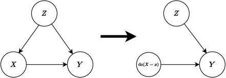
Figure 2: Illustration of the hypothesis that is being tested

In Figure 2, we first consider the graphical representation of the problem of establishing the relationship between $X$ and $Y$ under observed confounders $Z$. To adjust for confounders, we apply the do operation on our treatment $X$, in order to remove any dependency between $X$ and $Z$. The resulting distribution, which we denote $p(z,y\,|\,\text{\it do}(x))$, can be seen as the conditional distribution of $Y,Z$ given $X$ where we have made $Z$ and $X$ independent, but not affected the conditional distribution of $Y$ given $Z,X$. This distribution can then be used to understand the causal relationship between $X$ and $Y$.

To derive this expression, consider observations $\left\{(x_{i},y_{i},z_{i})\right\}_{i=1}^{n}\sim p$, where $p$ is some probability density on the joint space $\mathcal{X}\times\mathcal{Y}\times\mathcal{Z}$. We are interested in the do-conditional distribution

$$p^{*}(y|x)=p(y|do(x)) = \int p(y|\text{\it do}(x),z)p(z\,|\,\text{\it do}(x))dz$$

$$= \int p(y|\underbrace{x,z}_{\mathclap{\text{Only causal association between $x$ and $y$}}})p(z\,|\,\text{\it do}(x))dz$$

$$= \int p(y|x,z)p(\underbrace{z}_{\mathclap{\text{Dependency between $x$ and $z$ gone}}})dz.$$

This defines a joint density $p^{*}(x,y,z)=p^{*}(x)p(z)p(y|x,z)$, for some arbitrary density $p^{*}(x)$. However in the above case, the backdoor criterion (Pearl, 2009) is satisfied by the set of confounders $Z$, which implies that $p(y\,|\,\text{\it do}(x))$ admits this representation.

We are now ready to present the first link between HSIC and $p(y\,|\,\text{\it do}(x))$, as we are interested in expectations under $p^{*}$ using samples from $p$.

Proposition 1.

Consider continuous and bounded real-valued functions $f,g$. The covariance between $f(X)$ and $g(Y)$ under $p^{*}$ can be calculated as

$$\text{Cov}^{*}\left[f(X),g(Y)\right] = \mathbb{E^{*}}[f(X)g(Y)]-\mathbb{E}^{*}[f(X)]\mathbb{E}^{*}[g(Y)]$$

$$= \mathbb{E}[Wf(X)g(Y)]-\mathbb{E}[f(X)]\mathbb{E}[Wg(Y)],$$

where $W=p(X)/p(X|Z)$ (provided that $p(X|Z)>0,\forall X,Z$ s.t. $p(X)>0$ and the integrals exist). Using these weights we can now calculate any expectation term under $p^{*}$ in the covariance estimator.

Proof

We show that $\mathbb{E}^{*}[g(Y)]$ and $\mathbb{E}^{*}[f(X)g(Y)]$ indeed can be calculated as $\mathbb{E}[Wg(Y)]$ and $\mathbb{E}[Wf(X)g(Y)]$ respectively. To see this, we have that

$$\mathbb{E}[Wf(X)g(Y)] = \iiint f(x)g(y)\frac{p(x)}{p(x|z)}p(x,y,z)\,dx\,dy\,dz$$

$$= \iint f(x)g(y)p(x)\left(\int p(y|x,z)p(z)\,dz\right)dx\,dy$$

$$= \iint f(x)g(y)p(x)p^{*}(y|x)\,dxdy$$

$$= \mathbb{E}^{*}[f(X)g(Y)].$$

The case for $f(x)=1$ then also follows.  

In the above example, we will need to estimate importance weights $w_{i}$ from observations $x_{i}\in\mathcal{X}$ and $z_{i}\in\mathcal{Z}$ such that $w_{i}=p(x_{i})/p(x_{i}|z_{i})$. Under the do-null, we have that $\mathbb{E}[Wf(X)g(Y)]=\mathbb{E}[f(X)]\mathbb{E}[Wg(Y)]$.

3.2 Changing the marginal distribution of $X$

Consider the measure $Q^{*}(dx,dy)=Q(dx)P^{*}(dy|x)=Q(dx)\int P(dy|x,z)P(dz)$. We see that this is the measure being used to take expectations $\mathbb{E}^{*}[\cdot]$ if we select $Q(dx)=P(dx)$. However we will elaborate why there is a merit in considering different choices for $Q(dx)$ in Section 3.3. Our measure of interest is $P^{*}(dy|x)$, and note that this conditional distribution is the same in $Q^{*}$ for any choice of $Q(dx)$.

Proposition 2.

Given a density $q$ absolutely continuous with respect to $p$, and let $W^{q}=q(X)/p(X\,|\,Z)$ be integrable. Then define

$$\text{Cov}_{q^{*}}(f(X),g(Y))=\mathbb{E}[W^{q}f(X)g(Y)]-\mathbb{E}_{q}[f(X)]\mathbb{E}[W^{q}g(Y)]$$

for continuous, bounded and real-valued $f,g$. Then

$$\text{Cov}^{*}(f(X),g(Y))=0\;\text{for all}\;f,g\quad\iff\quad\text{Cov}_{q^{*}}(f(X),g(Y))=0\;\text{for all}\;f,g,$$

which also holds if and only if do-null $H_{0}$ holds.

Proof

The $\Longrightarrow$ direction:

$$\mathbb{E}\left[{W}f(X)g(Y)\right] = \iiint f(x)\,g(y)\,\frac{p(x)}{p(x\,|\,z)}\,p(x,y,z)\,dx\,dy\,dz$$

$$= \iint f(x)\,g(y)\,p(x)\underbrace{\left(\int p(y\,|\,x,z)p(z)dz\right)}_{\text{under }H_{0}}\,dx\,dy$$

$$= \iint f(x)\,g(y)\,p(x)\,p(y)\,dx\,dy$$

$$= \mathbb{E}[f(X)]\mathbb{E}[g(Y)].$$

Using $W^{q}$ instead yields

$$\mathbb{E}\left[{W}^{q}f(X)g(Y)\right] = \iiint f(x)\,g(y)\,\frac{q(x)}{p(x\,|\,z)}\,p(x,y,z)\,dx\,dy\,dz$$

$$= \iint f(x)\,g(y)\,q(x)\underbrace{\left(\int p(y\,|\,x,z)p(z)dz\right)}_{\text{under }H_{0}}\,dx\,dy$$

$$= \iint f(x)\,g(y)\,q(x)\,p(y)\,dx\,dy$$

$$= \mathbb{E}_{X_{q}}[f(X)]\mathbb{E}[g(Y)].$$

It is trivial to see that the converse direction holds under the do-null as the selection of $q(x)$ only determines the marginal distribution and does not affect $p^{*}(y\,|\,x)$.  
Note here that the centering needs to be done for the new marginals, $q(x)$ and $q^{*}(y)=\int q^{*}(x,y)dx$ if we wish to estimate covariance under $q^{*}$. Calculating the covariance between two arbitrary functions can generally be tricky and may require parametric assumptions. This is obviously undesirable, so similarly to HSIC, we will consider cross-covariance operators, which represent the covariances between two functions of the variables. The key object of interest is the cross-covariance operator of treatments $X$ and outcomes $Y$ under $q^{*}$ distribution, which we denote by $C_{q^{*}}$. This operator plays analogous role to that of the cross-covariance under observational distribution $p$ in standard independence testing. In particular, the squared HS norm of $C_{q^{*}}$ is the population HSIC under $q^{*}$ and hence the size of this operator measures departure from the do-null hypothesis. Similarly to HSIC, whenever we use characteristic kernels, we have that $\|C_{q^{*}}\|^{2}=0\iff p(y)=p(y\,|\,\text{\it do}(x))$. Of course, we are unable to estimate this quantity directly since we do not have access to samples from $q^{*}$. The following immediate corollary to Proposition 2 relates $C_{q^{*}}$ to expectations under $p$.

Corollary 1.

The cross-covariance operator $C_{q^{*}}$ of $X$ and $Y$ under $q^{*}$ satisfies

$$\langle f,C_{q^{*}}g\rangle=\mathbb{E}[W^{q}f(X)g(Y)]-\mathbb{E}[f(X)]\mathbb{E}[W^{q}g(Y)],\;\forall f\in\mathcal{H}_{\mathcal{X}},g\in\mathcal{H}_{\mathcal{Y}}.$$

and $C_{q^{*}}$ can be expressed as

$$C_{q^{*}}:=\mathbb{E}[W^{q}k(X,\cdot)\otimes l(Y,\cdot)]-\mathbb{E}[k(X^{q},\cdot)]\otimes\mathbb{E}[W^{q}l(Y,\cdot)]$$

with $W^{q}_{i}=\frac{q(X_{i})}{p(X_{i}\,|\,Z_{i})}$.

Following this corollary, we can empirically estimate $C_{q^{*}}$ using the following expression:

$$\hat{C}_{q^{*}}=\frac{1}{n}\sum_{i=1}^{n}\tilde{w}_{i}k(\cdot,x_{i})\otimes l(\cdot,y_{i})-\left(\frac{1}{n}\sum_{j=1}^{n}k\left(\cdot,x_{j}^{q}\right)\right)\otimes\left(\frac{1}{n}\sum_{i=1}^{n}\tilde{w}_{i}l\left(\cdot,y_{i}\right)\right),$$ (2)

where $\left\{\left(x_{i},y_{i},z_{i}\right)\right\}_{i=1}^{n}\sim p(x,y,z)$ and $\left\{x_{j}^{q}\right\}\sim q$. In the case where both $q(x_{i})$ and $p(x_{i}|z_{i})$ are known, one would simply use the “true weights” $w_{i}=\frac{q(x_{i})}{p(x_{i}|z_{i})}$. We can show that the resulting estimator (2) is consistent.

Theorem 1.

Assuming $\text{Var}\left(\frac{q(X)}{p(X\mid Z)}\right)<\infty$, and that $\mathbb{E}_{X,X^{\prime}}[k(X,X^{\prime})]<\infty$, $\mathbb{E}_{Y,Y^{\prime}}[l(Y,Y^{\prime})]<\infty$, then $\hat{C}_{q^{*}}$ using true weights is a consistent estimator of $C_{q}$ and satisfies

$$\mathbb{E}\left[\|C_{q^{*}}-\hat{C}_{q^{*}}\|^{2}_{\mathrm{HS}}\right]=\mathcal{O}\left(\frac{1}{n}\right).$$

Proof

See Section A.1.  
In practice, however, the true weights would typically not be available and they would need to be estimated using density ratio estimation techniques, which we shall discuss in detail in Section 4. The weights estimation corresponds to estimating a function $h$, s.t. $\tilde{w}_{i}=h(x_{i},z_{i})$. We note that estimating $h$ will need to be performed on a different dataset than the one used to estimate the covariance in (2), to ensure independence between $h$ and $\left\{\left(x_{i},y_{i}\right)\right\}_{i=1}^{n}$. We now give a result regarding the convergence rate when density ratios are being estimated.

Theorem 2.

Under the conditions of Theorem 1 and assuming that $\hat{h}_{n}(x,z)$ is a consistent estimator of the density ratio $\frac{q(x)}{p(x\,|\,z)}$ with uniform convergence rate $\mathcal{O}(\frac{1}{n^{\alpha}})$ for $\alpha>0$, i.e.

$$\lim_{n\to\infty}\sup_{x,z}\left|\hat{h}_{n}(x,z)-{\frac{q(x)}{p(x\,|\,z)}}\right|\propto\mathcal{O}\left(\frac{1}{n^{\alpha}}\right).$$

Then

$$\mathbb{E}\left[\left\|C_{q^{*}}-\hat{C}_{q^{*}}\right\|^{2}_{\mathrm{HS}}\right]=\mathcal{O}\left(\frac{1}{n^{\min(1,\alpha)}}\right).$$

Proof

See Section A.2.  
In summary, the convergence rate for the bd-HSIC estimator using estimated weights is at worst the slower rate between estimator and the pointwise convergence rate of the weight estimates. Now that we have established how to estimate the cross-covariance operator $C_{q^{*}}$, analogously to HSIC, we will use the squared HS norm of $\hat{C}_{q^{*}}$ as our test statistic.

Proposition 3.

Let $\circ$ denote the element-wise matrix product and $\mathbf{K}_{++}$ denote summing all elements in the matrix $\mathbf{K}$. The squared HS norm of estimator in (2) is given by

$$\|\hat{C}_{q^{*}}\|_{\text{HS}}^{2}=\frac{1}{n^{2}}\tilde{\mathbf{w}}^{\top}\left(\mathbf{K}\circ\mathbf{L}\right)\tilde{\mathbf{w}}+\frac{1}{n^{4}}(\mathbf{K}^{Q})_{++}(\mathbf{L}\circ\tilde{\mathbf{W}})_{++}-\frac{2}{n^{3}}\cdot\tilde{\mathbf{w}}^{\top}\left(\mathbf{K}^{q}\mathbf{1}_{n}\circ\mathbf{L}\tilde{\mathbf{w}}\right)$$

where $\tilde{\mathbf{w}}=[h(x_{1},z_{1}),\ldots,h(x_{n},z_{n})]$, $\tilde{\mathbf{W}}=\tilde{\mathbf{w}}^{\top}\tilde{\mathbf{w}}$, $\mathbf{K}=[k(x_{i},x_{j})]_{i,j=1}^{n}$, $\mathbf{L}=[l(y_{i},y_{j})]_{i,j=1}^{n}$, $\mathbf{K}^{Q}=[k(x^{q}_{i},x^{q}_{j})]_{i,j=1}^{n}$,$\mathbf{K}^{q}=[k(x_{i},x^{q}_{j})]_{i,j=1}^{n}$ and $\mathbf{1}_{n}$ is a vector of ones with length $n$.

Proof

See Section B.  
The above expression can be viewed as a weighted version of HSIC. We note that a weighted form of HSIC has previously been considered in a different context – when testing for independence on right-censored data (Rindt et al., 2020).

3.3 The choice of the $q$-marginal

Using $q(x)$ vs $p(x)$

In general, we would expect $q(x)$ to provide a higher effective sample size of $w$’s if chosen appropriately. To maximize effective sample size we can choose $q(x)$ such that it would be the resulting distribution if we took $x_{i}^{q}\sim q(x)$ as $x_{i}^{q}=c_{q}\cdot x_{i}$. For continuous $x_{i}$ with mean 0, this can be viewed as scaling the variance of samples $x_{i}$. We illustrate this in Figure 3.

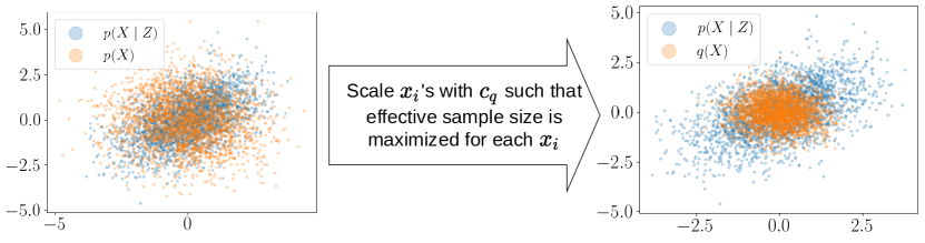
Figure 3: In the left example plot, $p(X)$ has samples where $p(X\,|\,Z)$ has little support. By constructing $q(X)$, samples from $q(X)$ has support where $p(X\,|\,Z)$ has support yield a higher effective sample size.

We describe how to choose an optimal $c_{q}$ for continuous densities in the paragraphs below.

Rule based selection of $c_{q}$

To find an optimal $c_{q}$ for univariate and multivariate $X,Z$, we optimize the effective sample size of $w_{i}=\frac{q(x_{i})}{p(x_{i}\,|\,z_{i})}$. The effective sample size is optimized to make the test-statistic have as much power as possible. Since the marginals of $X,Z$ are generally unknown, we derive a heuristic based on Gaussian distributions.

Proposition 4.

Assuming standard normal marginals for univariate $X,Z$ with correlation $\rho$ we choose the $c_{q}$ such that the effective sample size (ESS)

$$\text{ESS}:=\frac{\left(\sum_{i}w_{i}\right)^{2}}{\sum_{i}w_{i}^{2}}$$

is maximized, where $w_{i}$ is the weight used to re-sample observations. The optimal $c_{q}$ is then given by $c_{q}=\sqrt{1-2\rho^{2}}$.

Proof

See Section C.1.  
Here the optimal $c_{q}$ is found analytically.

Proposition 5.

Assuming $\left(X,Z\right)\sim\mathcal{N}_{p+q}(0,\Sigma)$, where we take $\Sigma=\begin{bmatrix}\Sigma_{xx}&\Sigma_{xz}\\ \Sigma_{zx}&\Sigma_{zz}\end{bmatrix}$ and assume that $\Sigma_{xx}=I_{p}$ and $\Sigma_{zz}=I_{q}$, the optimal new covariance matrix is found by maximizing the quantity

$$\operatorname{det}(D)\operatorname{det}\left(2T^{-1}-\left(I_{p}-\Sigma_{xz}\Sigma_{zx}\right)^{-1}-BD^{-1}B^{\top}\right)$$

with respect to the positive definite matrix $T$, where $B:=\left(I_{p}-\Sigma_{xz}\Sigma_{zx}\right)^{-1}\Sigma_{xz}$ and $D:=I_{q}-\Sigma_{zx}\left(I_{p}-\Sigma_{xz}\Sigma_{zx}\right)^{-1}\Sigma_{xz}$.

Proof

See Section C.2.  
In practice in the multivariate case, we choose $T=I_{p}\cdot c_{q}$, and perform the optimization using gradient descent.

4 Estimation of Weights

Since we will generally never have access to the true weights needed for backdoor adjustment, we need to estimate them from observed data. We denote estimated weights as $\tilde{w}_{i}$. In this section, we describe how to estimate these $\tilde{w}_{i}$ for both categorical and continuous $X$.

4.1 Categorical treatment variable $X$

For categorical $x_{i}$ we estimate $w_{i}$ using the ratio $\frac{q(x_{i})}{p(x_{i}\,|\,z_{i})}$, where we take $q(x)=p(x)$. We first estimate $p(x)$ by simply taking the empirical probabilities for each category using the training data. For $p(x\,|\,z)$, we fit a probabilistic classifier mapping from $z$ to each class of $x$. When $X$ consists of multiple categorical dimensions, i.e. $d_{X}>1$, we consider the $q(x)$ and $p(x\,|\,z)$ over the joint space of $\mathcal{X}_{1}\times\ldots\times\mathcal{X}_{d_{X}}$. In the cases where $d_{X}$ is large ($\geq 8$), we assume each $x_{d}$ to be independent of each other and take $p(x)=\prod_{d=1}^{d_{X}}p(x_{d})$ and $p(x\,|\,z)=\prod_{d=1}^{d_{X}}p(x_{d}\,|\,z)$.

4.2 Continuous treatment variable $X$

In the continuous case, we can no longer estimate $p(x\,|\,z)$ or $q(x)$ using a classifier straightforwardly. This complicates the estimation of the density ratio $w=\frac{q(x)}{p(x\,|\,z)}$, as we could either estimate $q(x)$ and $p(x\,|\,z)$ separately using density estimation or estimate the density ratio directly. We review some existing methods below.

Direct density estimation of $q(x)$ and $p(x\,|\,z)$ allows for a broad range of methods such as Normalizing flows (Rezende and Mohamed, 2015), Generative Adversarial Networks (Goodfellow et al., 2014) and Kernel Density Estimation (Botev et al., 2010) among many. While these methods provide accurate density estimation, they tend to be computationally expensive and hard to train (Mescheder et al., 2018). In this paper, we do not explore them further since densities themselves are not of direct interest.

RuLSIF (Yamada et al., 2011) propose using Kernel Ridge Regression to directly estimate the density ratio $r(x)=\frac{p_{1}(x)}{p_{2}(x)}$ between distributions $p_{1}(x)$ and $p_{2}(x)$. While this method offers an analytical approach to estimating the density ratio, a regression may often not be flexible enough to learn our density ratio of interest in a high dimensional setting. We compare against RuLSIF in the experiment section.

Noise Contrastive Density Estimation (NCE) (Gutmann and Hyvärinen, 2012) considers the problem of estimating an unknown density $p_{\text{true}}(\mathbf{x};\theta)$ with parameters $\theta$ from samples $\mathbf{x}\in\mathbb{R}^{d}$. The key idea of NCE is to convert a density estimation problem to a classification problem by selecting an auxiliary noise contrastive distribution $p_{\text{noise}}(\mathbf{x})$ to compare with samples from $p_{\text{true}}$. This noise contrastive distribution is used to train a density ratio $\hat{p}(\mathbf{x};\theta^{\prime})$ with parametrization $\theta^{\prime}$ of $p_{\text{true}}$ to distinguish between fake samples $\mathbf{z}\sim p_{\text{noise}}$ and observations $\mathbf{x}_{i}\sim p_{\text{true}}$ through binary classification. We can then derive $p_{\text{true}}$ by using this estimated density ratio. NCE has numerous desirable properties, including consistency under mild assumptions. We will propose and use a slightly modified NCE method to estimate our desired density ratio. We detail this method in the next section.

Telescoping Density Ratio (TRE) (Rhodes et al., 2020) considers the problem of estimating the density ratio between distributions $p_{0}$ and $p_{m}$ using samples $\mathbf{x}_{0}\sim p_{0}$ and $\mathbf{x}_{m}\sim p_{m}$. However, these density ratio problems tend to become pathological when $p_{0}$ and $p_{m}$ are too far apart, exhibiting a phenomenon coined density chasm. The main idea of TRE is then to decompose this density ratio into several sub-tasks through a telescoping product

$$\frac{p_{0}(\mathbf{x})}{p_{m}(\mathbf{x})}=\frac{p_{0}(\mathbf{x})}{p_{1}(\mathbf{x})}\frac{p_{1}(\mathbf{x})}{p_{2}(\mathbf{x})}\cdots\frac{p_{m-2}(\mathbf{x})}{p_{m-1}(\mathbf{x})}\frac{p_{m-1}(\mathbf{x})}{p_{m}(\mathbf{x})},$$

and estimate each individual ratio with separate estimators $r_{k}\left(\mathbf{x};\theta_{k}\right)\approx p_{k}(\mathbf{x})/p_{k+1}(\mathbf{x})$ for $k=0,\ldots,m-1$ and compose the original density ratio as

$$r(\mathbf{x};\theta)=\prod_{k=0}^{m-1}r_{k}\left(\mathbf{x};\theta_{k}\right)\approx\prod_{k=0}^{m-1}\frac{p_{k}(\mathbf{x})}{p_{k+1}(\mathbf{x})}=\frac{p_{0}(\mathbf{x})}{p_{m}(\mathbf{x})}.$$

To train each estimator $r_{k}\left(\mathbf{x};\theta_{k}\right)$ we require a gradual transformation of samples between $\mathbf{x}_{0}$ and $\mathbf{x}_{m}$, resulting in intermediate samples $\textbf{x}_{k}\sim p_{k},\quad k=0,\ldots,m-1$. We define these samples as a linear combination of $\textbf{x}_{0}$ and $\textbf{x}_{m}$

$$\mathbf{x}_{k}=\sqrt{1-\alpha_{k}^{2}}\mathbf{x}_{0}+\alpha_{k}\mathbf{x}_{m},\quad k=0,\ldots,m$$

where the $\alpha_{k}$’s form an increasing sequence from 0 to 1. The training objective

$$\mathcal{L}_{\mathrm{TRE}}(\theta) =\frac{1}{m}\sum_{k=0}^{m-1}\mathcal{L}_{k}\left(\theta_{k}\right)$$

$$\mathcal{L}_{k}\left(\theta_{k}\right) =-\mathbb{E}_{\mathbf{x}_{k}\sim p_{k}}\log\left(\frac{r_{k}\left(\mathbf{x}_{k};\theta_{k}\right)}{1+r_{k}\left(\mathbf{x}_{k};\theta_{k}\right)}\right)-\mathbb{E}_{\mathbf{x}_{k+1}\sim p_{k+1}}\log\left(\frac{1}{1+r_{k}\left(\mathbf{x}_{k+1};\theta_{k}\right)}\right)$$

is the average of all $m$ losses of the subtasks.

4.3 NCE for bd-HSIC

In the do-null context, we have access to samples $\left\{(x_{i},y_{i},z_{i})\right\}_{i=1}^{n}\sim p$. To calculate $\|\hat{C}_{q^{*}}\|^{2}$ we need to estimate the density ratio $\tilde{w}_{i}=\frac{q(x_{i})}{p(x_{i}|z_{i})}$ from our observations. Here $q(x)$ is a chosen marginal distribution of $X$. We can express the density ratio as

$$w_{i}=\frac{q(x_{i})}{p(x_{i}|z_{i})}=\frac{q(x_{i})p(z_{i})}{p(x_{i},z_{i})}.$$

If we take $q(x)=p(x)$, the problem translates into finding the density ratios between the product of the marginals and the joint density.

We can make use of the NCE framework by taking taking joint samples $D_{1}=\{(x_{i},z_{i})\}_{i=1}^{n}$ and approximate samples from the product of the marginals $D_{2}=\left\{\left(x_{i},z_{\pi(i)}\right)\right\}_{i=1}^{n}\sim p(x)p(z)$, for a randomly drawn permutation $\pi$. We obtain $D_{1}$ and $D_{2}$ by splitting the dataset to ensure independence between positive samples and negative samples in NCE.

By setting $p_{\text{true}}({x},z)=p(x,z)$ and $p_{\text{noise}}(x,z)=p(x)p(z)$, we can parametrize the noise contrastive classifier as $h(x,z;\theta)=\sigma(\ln{(\frac{1}{\nu}\frac{p(x)p(z)}{p(x,z;\theta)})})=\sigma(\ln{(\frac{1}{\nu}r(x,z;\theta))})$, where $r(x,z;\theta)$ is a classifier parametrized by $\theta$. By using NCE to directly estimate the density ratio between the product of the marginals and the joint density we gain the advantage that we do not need to specify an explicit noise contrastive distribution (and potentially introduce bias), as we can already obtain samples approximately through permutation. The problem is then reduced to a classification problem where we have to discriminate between samples from the product of marginals and the joint distribution. We introduce two modifications which take advantage of using the marginal $q(x)$.

NCE-$q$

Consider any $q(x)\neq p(x)$. We then build a classifier to discriminate between datasets $D_{1}=\left\{\left(x_{i},z_{i}\right)\right\}$ from $D_{2}^{q}=\{(x_{j}^{q},z_{j})\}$ where $\{x_{j}^{q}\}\sim q$ independently of $z_{j}$, so $D_{2}^{q}$ contains samples from $q(x)\,p(z)$. When we pass any new pair $(x,z)$ (i.e. regardless where it comes from, and in particular it can come from $p(x,z)$) to the classifier, it gives us the density ratio

$$\frac{q(x)p(z)}{p(x,z)}=\frac{q(x)}{p(x\,|\,z)},$$

which is then parametrized as

$$h(x,z;\theta)=\sigma\left(\ln{\left\{\frac{1}{\nu}\frac{q(x)p(z)}{p(x,z;\theta)}\right\}}\right)=\sigma\left(\ln{\left\{\frac{1}{\nu}r(x,z;\theta)\right\}}\right).$$

TRE-$q$

We can apply TRE to density ratio estimations between joint samples $\textbf{x}_{0}=\left(x,z\right)$ and product of marginals $\textbf{x}_{m}=\left(x^{q},z\right)$. For our particular context involving a chosen $q(x)$, we generate intermediate samples $\mathbf{x}_{k}=\left(\sqrt{1-\alpha_{k}^{2}}x+\alpha_{k}x^{q},z\right)$ by fixing $z$ for $k=0,\ldots,m$.

4.4 Mixed treatment $X$

When $X$ both contains continuous and categorical treatments, modifications to the continuous method are needed. We observe that if we take $X=x_{\text{cat}}\cup x_{\text{cont}}$ we have

$$w(x_{\text{cat}},x_{\text{cont}})=\frac{p(x_{\text{cat}},x_{\text{cont}})}{p(x_{\text{cat}},x_{\text{cont}}\,|\,z)} = \frac{p(x_{\text{cat}},x_{\text{cont}})}{p(x_{\text{cat}}\,|\,z,x_{\text{cont}})p(x_{\text{cont}}\,|\,z)}$$ (3)

$$= \underbrace{\frac{p(x_{\text{cat}}\,|\,x_{\text{cont}})}{p(x_{\text{cat}}\,|\,z,x_{\text{cont}})}}_{\text{Classifiers}}\cdot\underbrace{\frac{p(x_{\text{cont}})}{p(x_{\text{cont}}\,|\,z)}}_{\text{NCE}}.$$ (4)

We note that we can decompose the density ratio into a product of density ratios estimated using classifiers and density ratio estimation methods. We will use this as the main method for mixed treatment data since this composition allows us to simplify the problem by avoiding estimating density ratios over joint categorical and continuous treatment data which could induce density chasms Rhodes et al. (2020). We compare our proposed method to dimension-wise mixing, proposed in Rhodes et al. (2020). The same techniques can also be applied to NCE-q.

4.5 Algorithmic procedure

We describe the procedures in estimating weights $\tilde{w}$ and our proposed testing procedure.

Training the density ratio estimator

We train our density ratio estimators $r(x,z;\theta)$ through gradient descent. We parameterize all our estimators as Neural Networks (NN), due to their ability to fit almost any function. We summarize the training procedure for categorical data in Algorithm 1 and continuous data in Algorithm 2. We take our validation criteria in Algorithm 2 to be out-of-sample loss.

Input: Data $\mathcal{D}=\{x_{i},z_{i},x^{q}_{i}\}_{i=1}^{n//2}$

Output: Trained estimator $r(x,z;\theta^{\prime})$

Partition data into training and validation $\mathcal{D}=\mathcal{D}_{tr}\cup\mathcal{D}_{val}$

Initialise estimator $r(x,z,\theta^{\prime})$

if $D>8$ then

       for each categorical $x^{d}$ do

             Estimate $p(x^{d})$ using empirical probabilities

             Estimate $p(x^{d}\,|\,z)$ using a classifier with parameters $\theta_{d}$

             Set $r^{d}(x^{d},z;\theta_{d})=\frac{p(x^{d})}{p(x^{d}\,|\,z;\theta_{d})}$

       end for

      Set $r(x,z)=\prod_{d=1}^{n}r^{d}(x^{d},z;\theta_{d})$

end if

else

       Estimate $p(x)$ over joint space

       Estimate $p(x\,|\,z)$ using a classifier $\theta$

       Set $r(x,z)=\frac{p(x^{d})}{p(x^{d}\,|\,z;\theta)}$

end if

Return: Trained estimator $r(x,z)$

Algorithm 1 Training a density ratio estimator for categorical $X$

Input: Data $\mathcal{D}=\{x_{i},z_{i},x^{q}_{i}\}_{i=1}^{n//2}$

Output: Trained estimator $r(x,z;\theta)$

Partition data into training and validation $\mathcal{D}=\mathcal{D}_{tr}\cup\mathcal{D}_{val}$

Initialize estimator $r(x,z,\theta)$

Partition data into joint and product of the margin samples $\mathcal{D}_{tr}=\mathcal{D}_{tr}^{1}\cup\mathcal{D}_{tr}^{2}$, $\mathcal{D}_{val}=\mathcal{D}_{val}^{1}\cup\mathcal{D}_{val}^{2}$

while validation criteria $\nu$ not converged do

       Sample positive and negative samples $\delta_{+}\subset\mathcal{D}_{tr}^{1},\delta_{-}\subset\mathcal{D}_{tr}^{2}$;

       Calculate loss $l=\mathcal{L}(r(\delta_{+}),r(\delta_{-}))$;

       Gradient Descent $\theta=\theta+\frac{\partial l}{\partial\theta}$;

       Calculate validation loss $\mathcal{L}(r(\mathcal{D}_{val}^{1}),r(\mathcal{D}_{val}^{2}))$;

      

end while

Return: Trained estimator $r(x,z)$

Algorithm 2 Training a NCE-based density ratio estimator

Testing procedure

The entire procedure of the test can be summarized in Algorithm 3. It should be noted that when we carry out the permutation test, we permute on $\mathbf{L}$ in equation 7.

Input: Data $\left\{(x_{i},y_{i},z_{i})\right\}_{i=1}^{n}$, Distribution $q(x)$, density ratio estimator $r(\cdot)$

, number of permutations $n_{q}$

Output: p-value for $H_{0}$

Find optimal $c_{q}$ for continuous $X$

Sample $\{x^{q}_{i}\}^{n}_{i=1}\sim q$

Partition data into $\mathcal{D}_{1}=\left\{(x_{i},y_{i},z_{i},x^{q}_{i})\right\}_{i=1}^{\lfloor{n/2}\rfloor+1}$ and $\mathcal{D}_{2}=\left\{(x_{i},y_{i},z_{i},x^{q}_{i})\right\}_{i=\lfloor{n/2}\rfloor+1}^{n}$

Train $r$ on $\mathcal{D}_{1}$

Get weights $\{\tilde{w}_{i}\}_{i=\lfloor{n/2}\rfloor+1}^{n}=r(\left\{(x_{i},z_{i},x^{q}_{i})\right\}_{i=\lfloor{n/2}\rfloor+1}^{n})$

Calculate $\|\hat{C}_{q^{*}}\|^{2}$ using $\mathcal{D}_{2}$

Calculate permuted test-statistics $\Lambda=\{\|\hat{C}_{q^{*}}\|^{2}_{1},\ldots,\|\hat{C}_{q^{*}}\|^{2}_{n_{q}}\}$

Calculate the p-value as $p=2\min\left(1-\frac{1+|\|\hat{C}_{q^{*}}\|^{2}<\Lambda\mid}{1+\mid\Lambda\mid},\frac{1+\mid\|\hat{C}_{q^{*}}\|^{2}<\Lambda\mid}{1+\mid\Lambda\mid}\right)$

Return: $p$

Algorithm 3 Testing $H_{0}:p(y\,|\,\text{\it do}(x))=p(y)$

It should be noted that we partition the data such that the data used for estimation of weights is independent of the data used for the permutation test.

5 Simulations

We run experiments using bd-HSIC in the following contexts of do-null testing:

1. Linear $X,Y$ dependencies under multiple treatments and treatment types, multiple confounders and multiple outcomes

2. Non-linear $X,Y$ dependencies under multiple treatments, multiple confounders and multiple outcomes

To nuance the exposition of bd-HSIC, we contrast against PDS, which serves as a representative benchmark with pathologies (including, but not limited to the g-null paradox) bd-HSIC attempts to amend.

Comparison against parametric methods

Given the above contexts, the coverage of PDS includes linear $X,Y$ dependencies with multiple treatments under multiple confounders.

To make comparisons straightforward, we only compare to PDS in univariate treatment, confounder and outcome cases. We further compare to $\tilde{w}_{i}\sim\text{Uniform}(0,1)$. While this choice of weights is not a very principled approach, it serves as a reference to see whether bd-HSIC actually needs correctly estimated weights to have power.

Studying the calibration under $H_{0}$

When the null hypothesis is true, we would expect the p-value distribution of the test run on several datasets to have the correct size. Here we use level $\alpha=0.05$.

Studying the power under $H_{1}$

Under the alternative, a desired property is high power across all parameters of the data generation. We will conduct experiments to demonstrate when the test has high power and when it does not. We calculate power for level $\alpha=0.05$.

5.1 Results

We divide our experiments into two steps: we first take the true weights and use them in the subsequent permutation test for bd-HSIC. In this initial step, we chose $q=p$. This is intended as a unit test to validate that the parameter selection used for data generation is working. It should be noted that generally the choice of $q$ and estimation of $c_{q}$ must be done cautiously to avoid double use of data.

In the second step we estimate weights from the data, and investigate the effectiveness of our proposed density ratio estimation procedure. We consider following methods for weight estimation: RuLSIF, random uniform, NCE-q and TRE-q as described in Section 4.3 and Section 4.

5.1.1 Binary treatment $X$

We simulate univariate binary data according to Section D.1. We vary the dependence $\beta_{XY}$ between $X$ and $Y$ to be $\{0.0,0.005,0.01,0.02,0.04,0.06,0.08,0.1\}$. We plot the power for the level $\alpha=0.05$ against the dependency between $X$ and $Y$, $\beta_{XY}$, in Figure 5.

$n=1000$

$n=5000$

$n=10000$

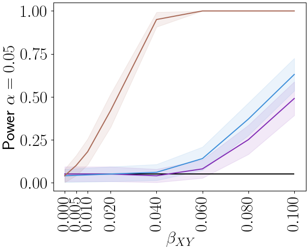
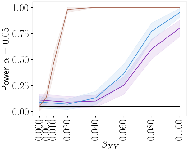
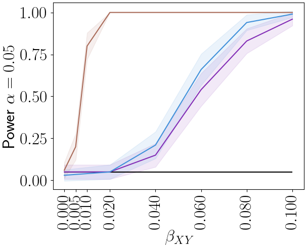
Figure 5: bd-HSIC(NCE-q):     bd-HSIC(true weights):     PDS:
Binary treatment for $n=1000,5000,10000$ using an RBF kernel in bd-HSIC. As the $p(Y|\text{\it do}(X=x))$ is linear, using a non-linear kernel provides less power.

5.1.2 Continuous treatment $X$

Linear dependency between $X$ and $Y$

The data are simulated for $(d_{z},d_{x},d_{y})\in\{(1,1,1),(3,3,3),(15,3,3),(50,3,3)\}$. In our experiments, we found that a strong confounding effect (i.e. large $\beta_{XZ}$) led to a smaller effective sample size, making it harder to obtain a consistent test under $H_{0}$. For $H_{1}$, the difficulty was mostly controlled by the magnitude of $\beta_{XY}$, where small magnitudes often led to a test with little or no power. We have chosen rejection sampling parameters $\theta,\phi,\beta_{XZ},\beta_{YZ}$ such that the tests are non-trivial but not a failure mode, where $\theta,\phi$ control variance of the marginal distribution of the treatment and the variance of proposal distribution respectively. For exact simulation details, we refer to the appendix. We consider $\beta_{XY}\in[0.0,0.05]$, with $\beta_{XY}=0.0$ corresponding to $H_{0}$. We illustrate how the linear dependency looks like in Figure 6. We present results for continuous treatment in Figure 8.

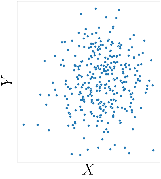
(a) $H_{0}:\beta_{XY}=0.0$

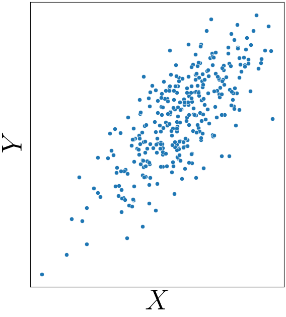
(b) $H_{1}:\beta_{XY}\neq 0.0$

Figure 6: Samples from $p^{*}$ under $H_{0}$ and $H_{1}$. Here the dependency is linear. It should be noted that samples from $p^{*}$ under $H_{0}$ look the same regardless of which dependency we choose.

$d_{Z}=1$

$d_{Z}=3$

$d_{Z}=15$

$d_{Z}=50$

$n=1000$

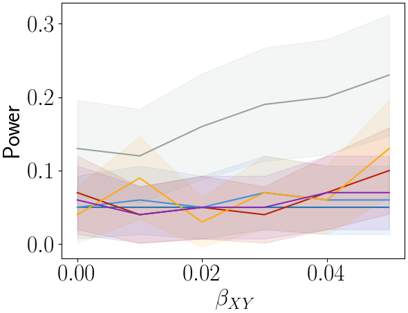
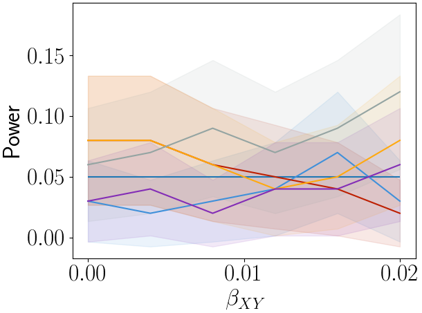
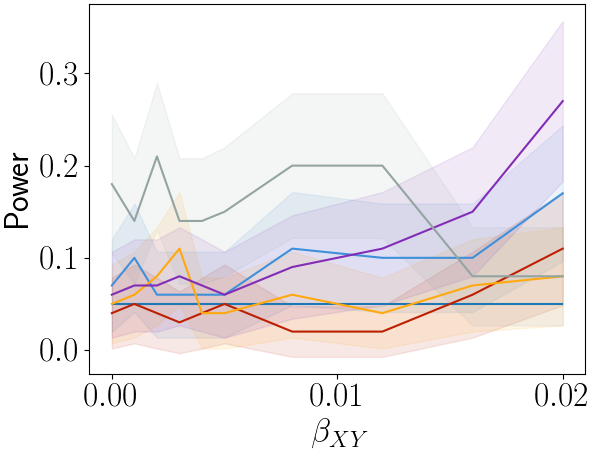
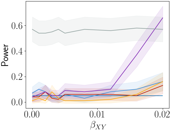
$n=5000$

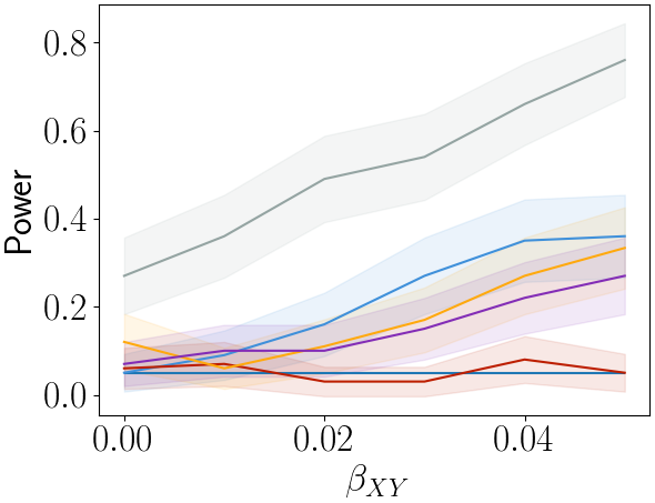
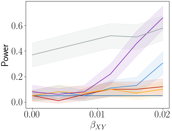
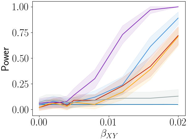
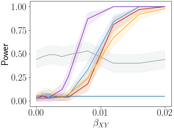
$n=10000$

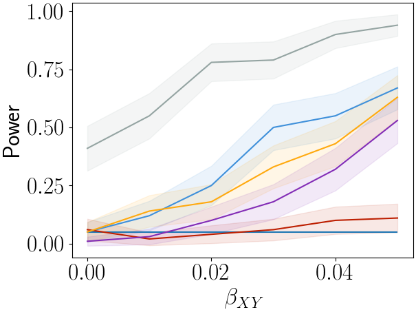
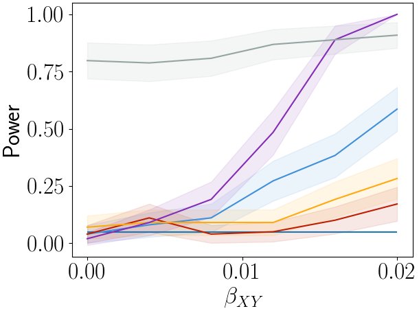
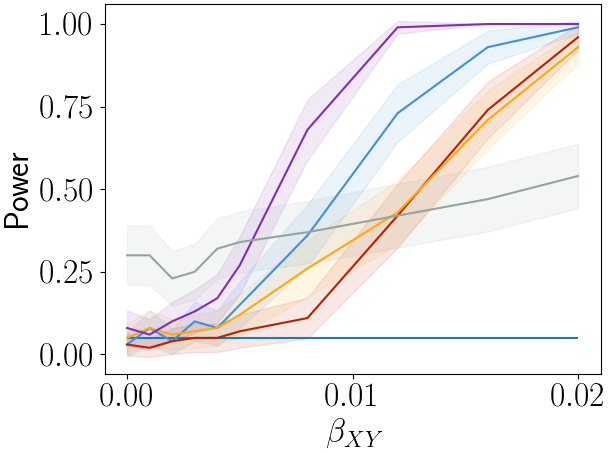
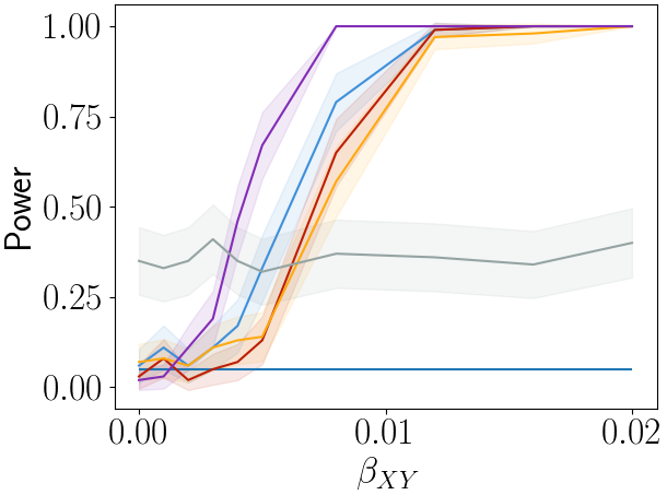
Figure 8: bd-HSIC(NCE-q):     bd-HSIC(TRE-q):     bd-HSIC(random uniform):     bd-HSIC(RuLSIF):     bd-HSIC(true weights):     PDS:
Continuous treatment results. We find that RuLSIF has incorrect size under the null and that uniform weights has less power. NCE-Q seems to have best power while being calibrated under the null. We generally note that random uniform weights have less or no power when compared to “true weights” and estimated weights.

Non-linear dependency between $X$ and $Y$

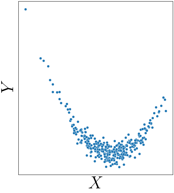
(a) U-shaped dependency, $Y=X^{2}\beta_{XY}$

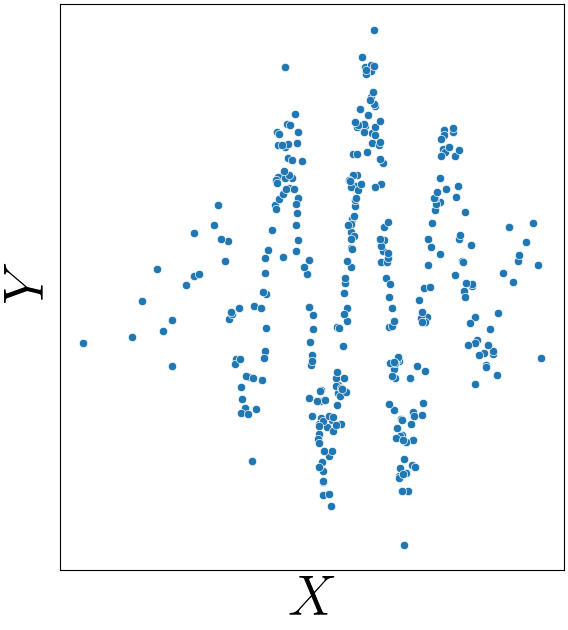
(b) General symmetric non-linear dependency, $Y=\exp(-0.1X^{2})\cos(X\pi)\beta_{XY}$

Figure 9: Samples from $p^{*}$ under $H_{1}$ where the dependency is non-linear.

Here we simulate data for $(d_{z},d_{x},d_{y})\in\{(1,1,1),(50,3,3)\}$ using the same parameters as in the linear case. The only difference now is that we consider a non-linear dependency between $X$ and $Y$ illustrated in Figure 9. Figure 9(a) illustrates a U-shaped dependency between $X$ and $Y$, which can be found in relationships between happiness vs. age (Kostyshak, 2017), and BMI vs. fragility (Watanabe et al., 2020) to name a few. The U-shaped dependency can be generalized to symmetric non-linear relationships between $X$ and $Y$ illustrated in Figure 9(b). We show the results in Figure 11 and Figure 13. We note that PDS has no power against the alternative when the dependency between $X$ and $Y$ is symmetric and non-linear, which is expected due to the linear nature of PDS.

$n=1000$

$n=5000$

$n=10000$

$d_{Z}=1$

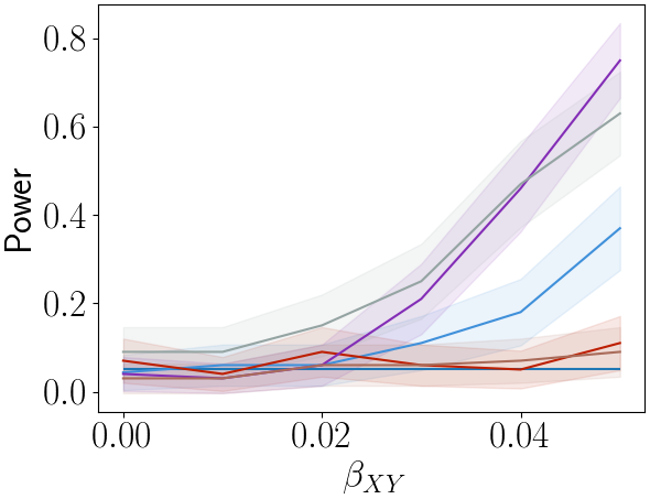
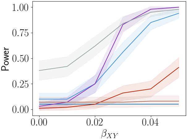
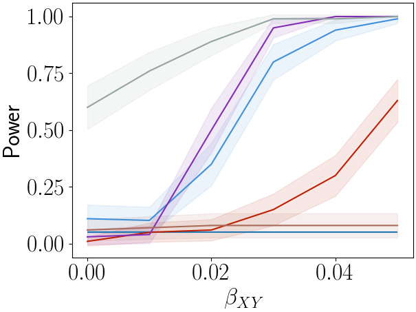
$d_{Z}=50$

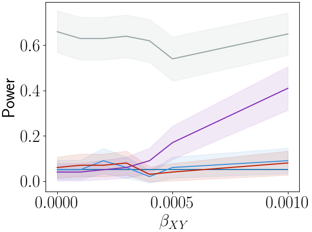
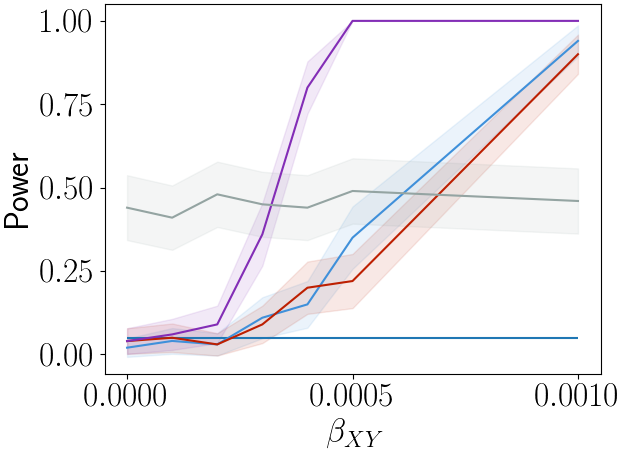
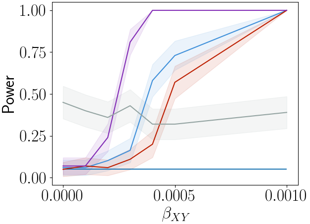
Figure 11: bd-HSIC(NCE-q):     bd-HSIC(random uniform):    bd-HSIC(RuLSIF):    bd-HSIC(true weights):    PDS:

Experiments for U-shaped dependency between $X$ and $Y$.

$n=1000$

$n=5000$

$n=10000$

$d_{Z}=1$

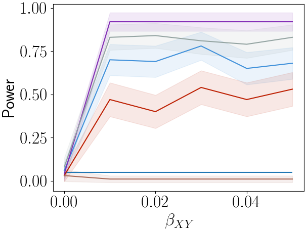
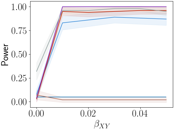
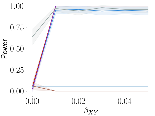
$d_{Z}=50$

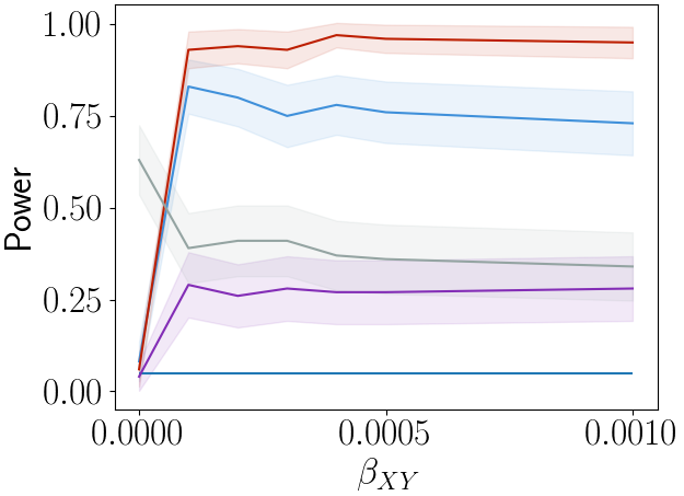
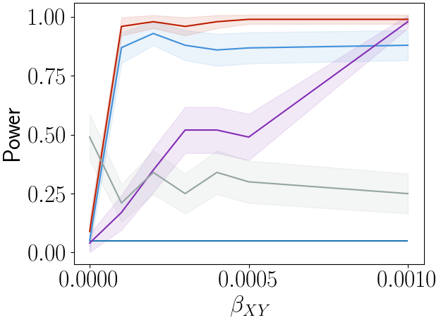
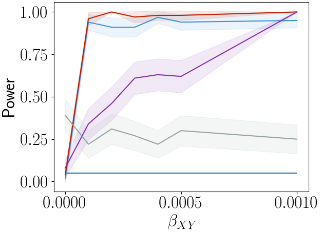
Figure 13: bd-HSIC(NCE-q):     bd-HSIC(random uniform):     bd-HSIC(RuLSIF):     bd-HSIC(true weights):     PDS:

Experiments for general non-linear symmetric dependency between $X$ and $Y$.

5.1.3 Mixed treatment $X$

The data are simulated for $(d_{z},d_{x},d_{y})\in\{(2,2,2),(4,4,3),(15,6,6),(50,8,8)\}$. We simulate the mixed data according to Algorithm D.3. Here we fix half of the $X$’s to be continuous and the other half binary. We consider $\beta_{XY}\in[0.0,0.1]$. We follow the same principles as in the continuous case when selecting $\theta,\phi,\beta_{XZ},\beta_{YZ}$.

In our experiments, we compare against RuLSIF and randomly sampled uniform weights. We also compare between estimating the density ratio of the binary treatments separately (denoted with suffix “prod”) and all treatments simultaneously (no suffix). The “mixed” suffix is a reference to the dimension-wise mixing proposed in Rhodes et al. (2020), which is applied when using TRE-Q. We present the results in Figure 15.

$d_{Z}=2$

$d_{Z}=15$

$d_{Z}=50$

$n=1000$

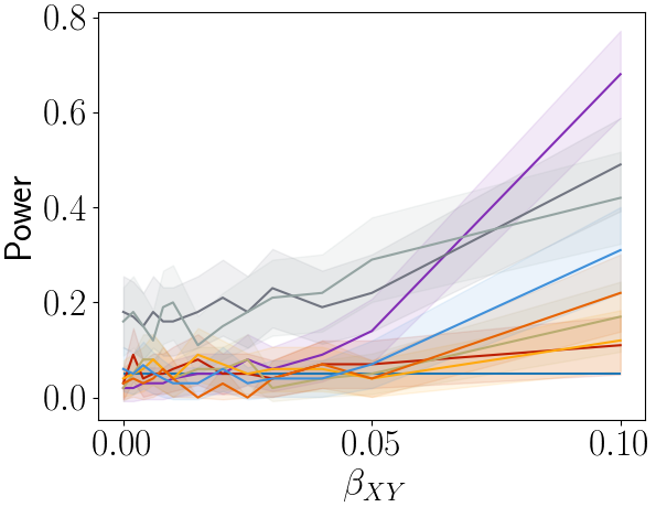
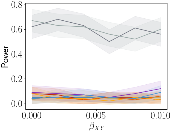
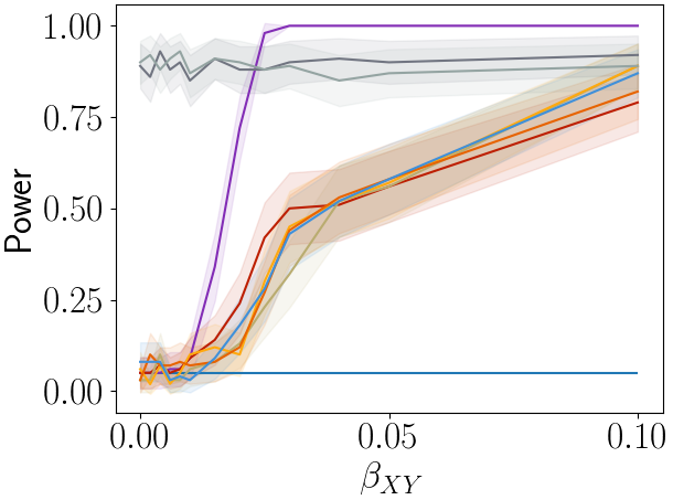
$n=5000$

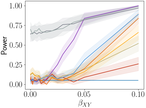
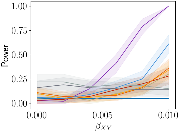
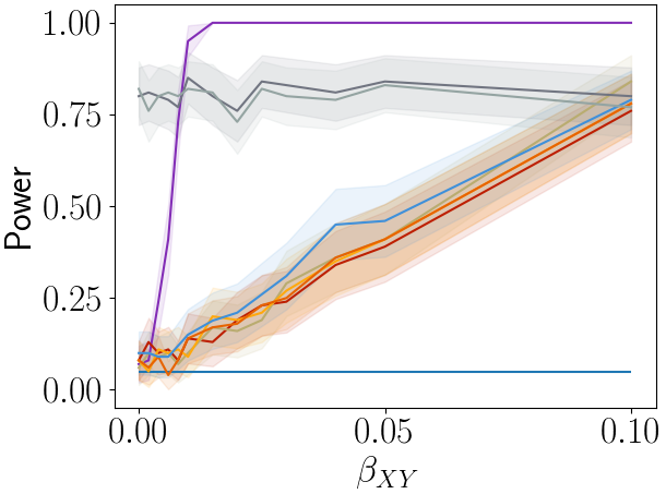
$n=10000$

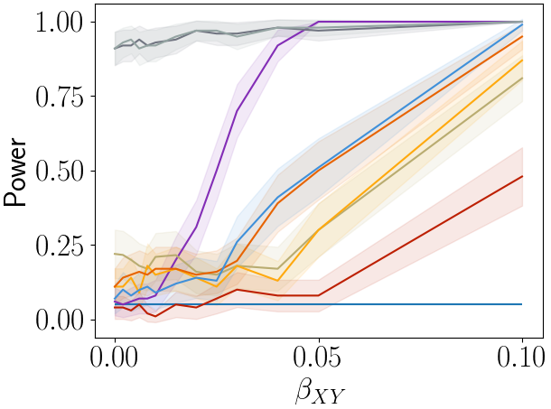
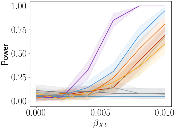
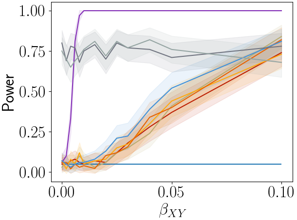
Figure 15: bd-HSIC(NCE-q, mixing):     bd-HSIC(TRE-q, mixing):     bd-HSIC(random uniform):     bd-HSIC(RuLSIF):     bd-HSIC(true weights):     bd-HSIC(NCE-q prod):     bd-HSIC(TRE-q product):     bd-HSIC(RuLSIF product):
Mixed treatment results. We find that RuLSIF has incorrect size under the null. TRE-q prod seems to have best power while being calibrated under the null.

5.2 The do-null is not marginal independence $X\perp Y$

We contrast the do-null against marginal independence $X\perp Y$, by constructing a dataset where the do-null is true, but there is marginal dependence between $X$ and $Y$. To construct such a dataset, we replace the normal marginal distributions for $X,Y,Z$ in Algorithm 4 with exponential distributions instead. For an illustration, see Figure 16(a).

We plot size ($\alpha=0.05$) against sample size when applying HSIC and bd-HSIC (true weights) in Figure 16(b). HSIC is not calibrated under the do-null.

5.3 The do-null is not conditional independence $X\perp Y\mid Z$

We similarly contrast the do-null against conditional independence $X\perp Y\mid Z$. We simulate a dataset such that there is a conditional dependence $X\not\perp Y\mid Z$ while the do-null is true. See Figure 16(c) for an illustration of the dependency between $X$ and $Y$. We apply the “RCIT” method, a kernel-based conditional independence test proposed in Strobl et al. (2019) and demonstrate that it is uncalibrated in relation to the do-null in Figure 16(d).

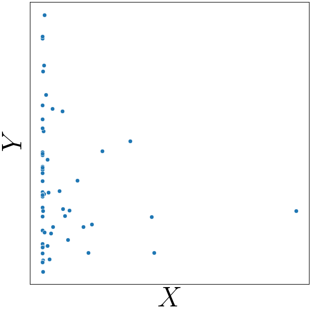
(a) Marginal dependency but true do-null, $Y=\exp(X\beta_{XY})$

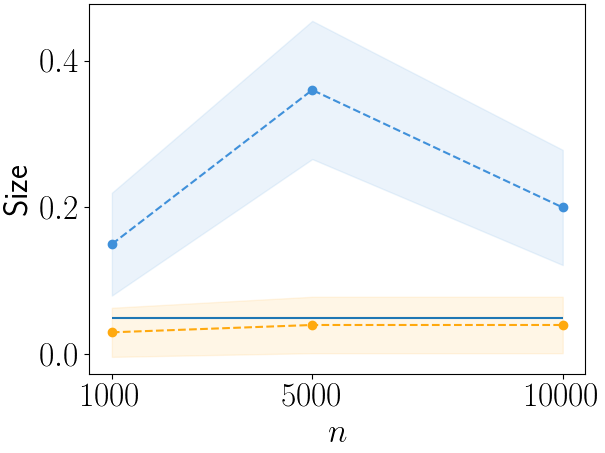
(b) bd-HSIC(true weights): vs HSIC:

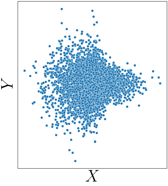
(c) Conditional dependency but true do-null, see code for more details

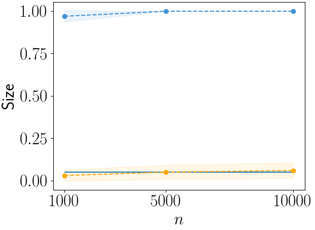
(d) bd-HSIC(true weights): vs RCIT:

5.4 Pitfalls

Choice of kernels, a cautionary tale

To improve the power of bd-HSIC, we could instead use a linear kernel. Figure 18 illustrates that bd-HSIC has comparable power to PDS, when using a linear kernel for testing the do-null when one considers the univariate binary treatment case.

$n=1000$

$n=5000$

$n=10000$

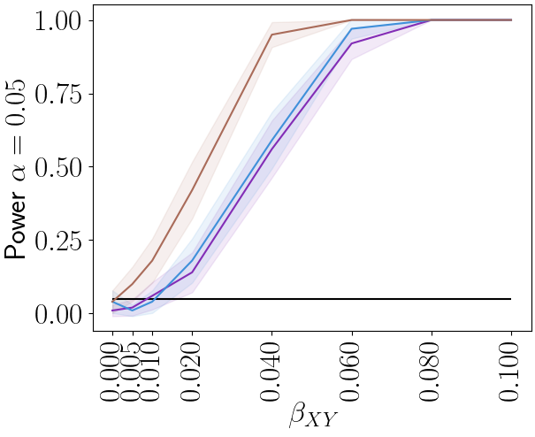
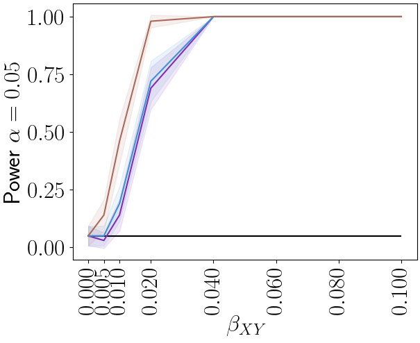
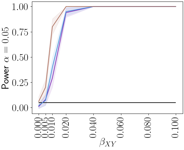
Figure 18: bd-HSIC(NCE-q):    bd-HSIC(true weights):    PDS:
Binary treatment for $n=1000,5000,10000$ using an linear kernel in bd-HSIC. Compared to Figure 5, bd-HSIC now has similar power to PDS.

However, when applying the linear kernel to univariate data for a continuous treatment the test becomes uncalibrated. In fact, the linear kernel makes bd-HSIC much more sensitive to confounding, exhibited in Figure 19(a).

When does bd-HSIC break?

We demonstrate a typical failure mode of bd-HSIC, when the value of $\beta_{XZ}$ is so strong that the density ratio estimation fails. We show that NCE-Q and TRE-Q has incorrect size when $\beta_{XZ}$ becomes large enough in Figure 19(b). Here we generate data under the null for $\beta_{XZ}=[0.0,0.05,0.1,0.15,0.25,0.5,0.75,1.0,1.5]$ for $d_{X}=d_{Y}=d_{Z}=3$.

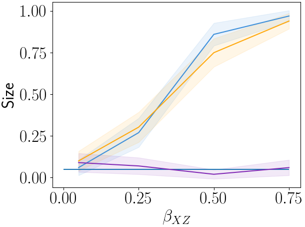
(a) Applying a linear kernel to univariate continuous treatment data. While true weights have the correct size, estimated density ratios do not.

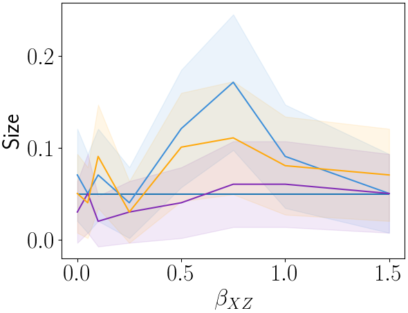
(b) bd-HSIC with estimated density ratios exhibits incorrect size for certain amount of confounding. True weights are consistent.

Figure 19: bd-HSIC(NCE-q):    bd-HSIC(TRE-q):    bd-HSIC(true weights):

5.5 Experiments on real data

Lalonde dataset experiments

The Lalonde dataset comes from a study that looked at the effectiveness of a job training program (the treatment) on the real earnings of an individual, a couple of years after completion of the program (the outcome). Each individual has several descriptive covariates such as age, academic background, etc., which confounds the treatment and the outcome. We compare the power between PDS and bd-HSIC on the Lalonde dataset in Figure 20. This is done by calculating the p-value on 100 bootstrap sampled subsets of the dataset. We further generate a random independent dummy outcome to verify that our tests are calibrated. We note that both PDS and bd-HSIC have the correct type I control for dummy outcome, while their power is comparable for the real earnings outcome.

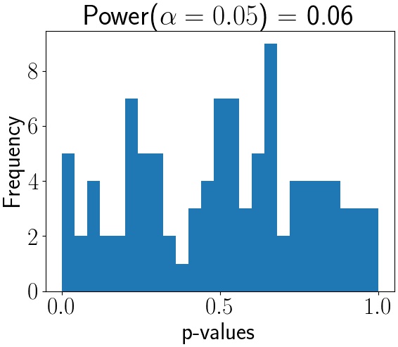
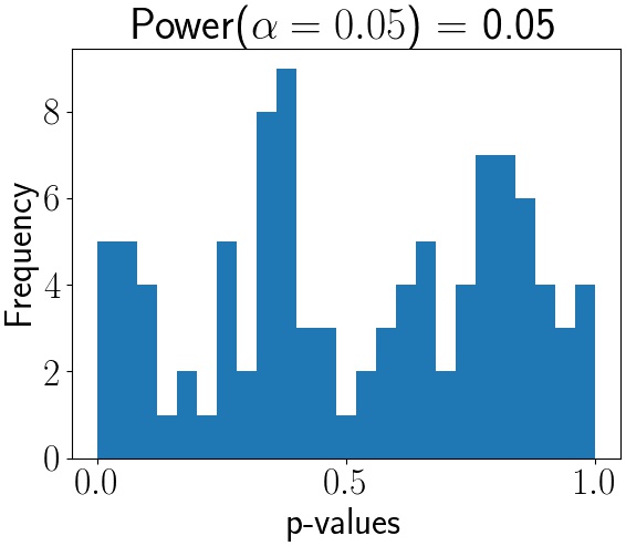
(a) PDS vs bd-HSIC(TRE-Q) on a dummy outcome

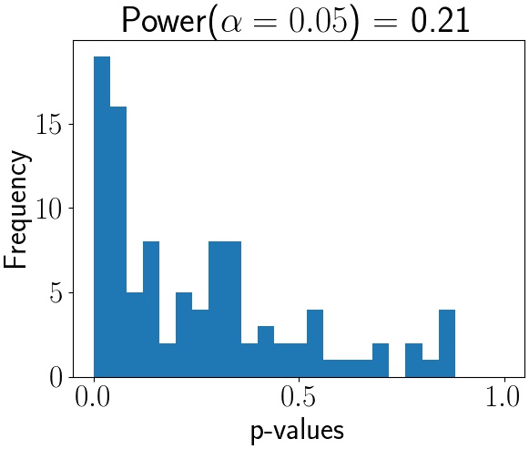
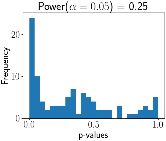
(b) PDS vs bd-HSIC(TRE-Q) on real earnings
 

Figure 20: Both methods are calibrated and provide adequate power

Twins dataset experiments

The twins dataset Louizos et al. (2017) considers data of twin births in the US between 1989–1991. Here the treatment is being born the heavier twin and the outcome is mortality. Besides treatment and outcome, there are also descriptive confounders such as smoking habits of the parents, education level of the parents, and medical risk factors of the children among many. For our experiments, we construct a slight variation of the experiment presented in Louizos et al. (2017), where we instead take the treatment to be $T=\left(\text{Weight}_{\text{heavier twin}},\text{Weight}_{\text{lighter twin}},\text{Weight}_{\text{heavier twin}}-\text{Weight}_{\text{lighter twin}}\right)$ and the outcome to be in the set $\{-1,0,1\}$, where $-1$ indicates that the lighter twin died, 1 that the heavier twin died, and 0 that either, neither or both died; everything else is kept the same. Similar to the Lalonde datasets we calculate the p-value on 100 bootstrap sampled subsets of the dataset and present results in Figure 21. Similar to the Lalonde dataset, we generated a random independent dummy outcome to verify that our tests are calibrated. Both methods suggests there exists a causal association between infant weight and mortality.

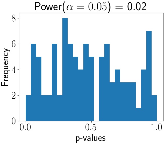
Dummy outcome Infant mortality

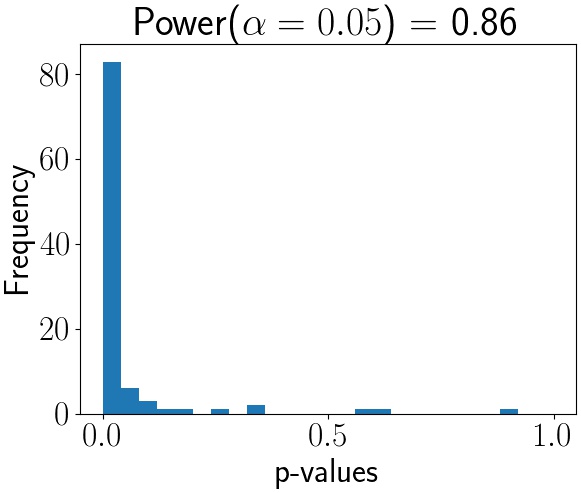
(a) PDS
 

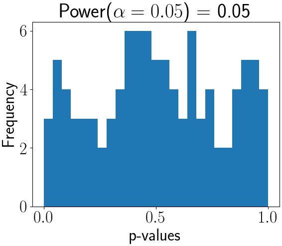
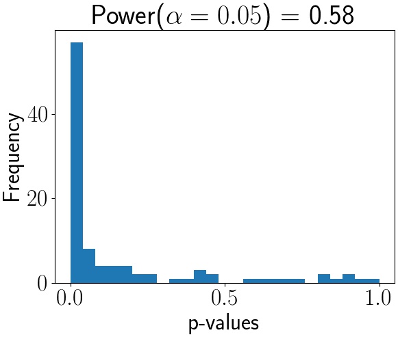
(b) bd-HSIC(TRE-q) – RBF kernel.

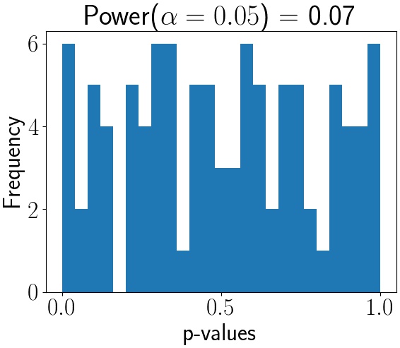
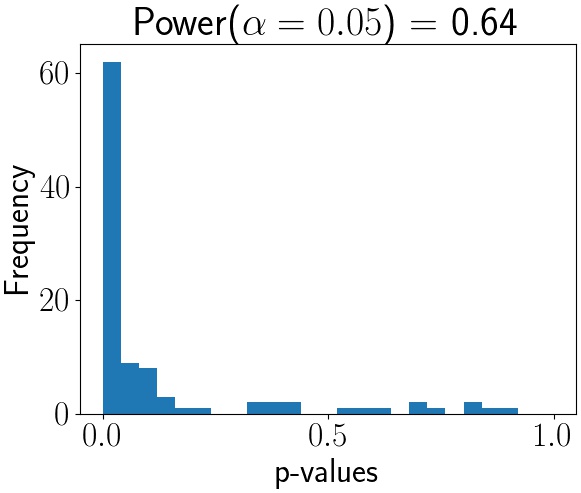
(c) bd-HSIC(TRE-q) – linear kernel.

Figure 21: PDS suggests that there exists a causal association between weight and mortality. This relationship appears to be linear: using a linear kernel slightly improves power.

6 Conclusion

We present a novel non-parametric method termed backdoor-HSIC (bd-HSIC), which is an importance weighted covariance-based statistic to test the causal null hypothesis, or do-null. We first show that our proposed estimator for bd-HSIC is consistent. Experiments on a variety of synthetic datasets, ranging from linear dependencies to non-linear dependencies with different numbers of confounders and treatments, show that bd-HSIC is a flexible method with wider coverage of scenarios compared to parametric methods such as PDS. Finally, we compare bd-HSIC to PDS on two real-world datasets, where bd-HSIC exhibits good power. A major benefit of bd-HSIC is that can serve as a powerful tool in causal inference as it complements parametric methods as PDS. For example, PDS generally has better power when the underlying dependency is linear but fails if the dependency is symmetrically non-linear. In these cases, bd-HSIC can be used as a complementary general test for non-linear causal association, which is of broad interest to all statistically inclined sciences.

By combining with kernel conditional independence tests, this work could be extended to testing for null conditional average treatment effects, as well as to testing more general nested independence constraints (Richardson et al., 2017).

A Consistency proofs

A.1 Proof of Theorem 1

Proof

We first define the kernel mean embeddings used in our proposed estimator:

$$\begin{split}\mathbb{E}[W^{q}k(x,\cdot)l(y,\cdot)]=\mu_{xy}(\cdot)&=\int W^{q}k(x,\cdot)l(y,\cdot)\,d\mathbb{P}_{\mathcal{X}\otimes\mathcal{Y}\otimes\mathcal{X}}(x,y,z)\\ &=\int\frac{q(x)}{p(x\,|\,z)}k(x,\cdot)l(y,\cdot)\,d\mathbb{P}_{\mathcal{X}\otimes\mathcal{Y}\otimes\mathcal{X}}(x,y,z)\end{split}$$

$$\mathbb{E}[k(x^{q},\cdot)]=\mu_{x^{q}}(\cdot)=\int k(x^{q},\cdot)\,d\mathbb{Q}(x)$$

$$\mathbb{E}[W^{q}l(y,\cdot)]=\mu_{y}(\cdot)=\int\frac{q(x)}{p(x\,|\,z)}l(y,\cdot)d\mathbb{P}_{\mathcal{X}\otimes\mathcal{Y}\otimes\mathcal{X}}(x,y,z).$$

Then we write the following for shorthand:

$$C_{q^{*}}=\mu_{xy}(\cdot)-\mu_{x^{q}}(\cdot)\otimes\mu_{y}(\cdot)$$

Thus

$$\mathbb{E}\left[\|C_{q^{*}}-\hat{C}_{q^{*}}\|^{2}_{\mathrm{HS}}\right]$$

Which is

$$\begin{split}&\mathbb{E}\Bigg{[}\Bigg{\|}\mu_{xy}(\cdot)-\mu_{x^{q}}(\cdot)\otimes\mu_{y}(\cdot)-\\ &\bigg{(}\underbrace{\frac{1}{n}\sum_{i=1}^{n}{\frac{q(x_{i})}{p(x_{i}\,|\,z_{i})}}k(\cdot,x_{i})\otimes l(\cdot,y_{i})}_{\hat{\mu}_{xy}}-\underbrace{\left(\frac{1}{n}\sum_{j=1}^{n}k\left(\cdot,x_{j}^{q}\right)\right)}_{\hat{\mu}_{x^{q}}}\otimes\underbrace{\left(\frac{1}{n}\sum_{i=1}^{n}{\frac{q(x_{i})}{p(x_{i}\,|\,z_{i})}}l\left(\cdot,y_{i}\right)\right)}_{\hat{\mu}_{y}}\bigg{)}\Bigg{\|}^{2}\Bigg{]}.\end{split}$$

Note that $w_{i}=\frac{q(x_{i})}{p(x_{i}|z_{i})}$, and for now we consider we have access to the true weights. Rearranging terms we get

$$\mathbb{E}\left[\left\|\underbrace{\mu_{xy}(\cdot)-\hat{\mu}_{xy}(\cdot)}_{A}+\underbrace{(\hat{\mu}_{x^{q}}(\cdot)\otimes\hat{\mu}_{y}(\cdot)-\mu_{x^{q}}(\cdot)\otimes\mu_{y}(\cdot))}_{B}\right\|^{2}\right]=\mathbb{E}\left[\langle A,A\rangle+2\langle A,B\rangle+\langle B,B\rangle\right].$$

The proof strategy is to obtain convergence rates for each term. First term $\langle A,A\rangle$:

$$\begin{split}\mathbb{E}\left[\langle A,A\rangle\right]&=\mathbb{E}\left[\langle\mu_{xy}(\cdot),\mu_{xy}(\cdot)\rangle\right]-2\mathbb{E}\left[\langle\mu_{xy}(\cdot),\hat{\mu}_{xy}(\cdot)\rangle\right]+\mathbb{E}\left[\langle\hat{\mu}_{xy}(\cdot),\hat{\mu}_{xy}(\cdot)\rangle\right]\end{split}$$

Let $x^{\prime},y^{\prime},z^{\prime}\sim p$ be an independent copy of $x,y,z\sim p$. The first term is then

$$\begin{split}\mathbb{E}\left[\langle\mu_{xy}(\cdot),\mu_{x^{\prime}y^{\prime}}(\cdot)\rangle\right]=\mathbb{E}_{x,y,z,x^{\prime},y^{\prime},z^{\prime}}\left[{\frac{q(x)}{p(x\,|\,z)}}{\frac{q(x^{\prime})}{p(x^{\prime}\,|\,z^{\prime})}}k(x,x^{\prime})l(y,y^{\prime})\right],\end{split}$$

the second one:

$$\mathbb{E}\left[\langle\mu_{xy}(\cdot),\hat{\mu}_{xy}(\cdot)\rangle\right] =\mathbb{E}\left[\frac{1}{n}\sum_{i=1}^{n}{\frac{q(x_{i})}{p(x_{i}\,|\,z_{i})}}\mathbb{E}_{x,y,z}\left[{\frac{q(x)}{p(x\,|\,z)}}k(x,x_{i})l(y,y_{i})\right]\right]$$

$$=\mathbb{E}_{x^{\prime},y^{\prime},z^{\prime}}\left[{\frac{q(x^{\prime})}{p(x^{\prime}\,|\,z^{\prime})}}\mathbb{E}_{x,y,z}[{\frac{q(x)}{p(x\,|\,z)}}k(x,x^{\prime})l(y,y^{\prime})]\right]$$

$$=\mathbb{E}_{x,y,z,x^{\prime},y^{\prime},z^{\prime}}\left[{\frac{q(x)}{p(x\,|\,z)}}{\frac{q(x^{\prime})}{p(x^{\prime}\,|\,z^{\prime})}}k(x,x^{\prime})l(y,y^{\prime})\right],$$

and the final one:

$$\mathbb{E}\left[\frac{1}{n^{2}}\sum_{i,j}w_{i}w_{j}k(x_{i},x_{j})l(y_{i},y_{j})\right]=\underbrace{\mathbb{E}\left[\frac{1}{n^{2}}\sum_{i\neq j}w_{i}w_{j}k(x_{i},x_{j})l(y_{i},y_{j})\right]}_{(a)}+\underbrace{\mathbb{E}\left[\frac{1}{n^{2}}\sum_{i}w_{i}^{2}k(x_{i},x_{i})l(y_{i},y_{i})\right]}_{(b)}.$$

Then $(a)$ is

$$(a)=\frac{(n-1)}{n}\mathbb{E}_{x,y,z,x^{\prime},y^{\prime},z^{\prime}}\left[{\frac{q(x)}{p(x\,|\,z)}}{\frac{q(x^{\prime})}{p(x^{\prime}\,|\,z^{\prime})}}k(x,x^{\prime})l(y,y^{\prime})\right].$$

(b):

$$\begin{split}(b)&=\frac{1}{n}\mathbb{E}\left[\left({\frac{q(x)}{p(x\,|\,z)}}\right)^{2}k(x,x)l(y,y)\right]\\ &\leq\frac{1}{n}\underbrace{\sup_{x\in X}k(x,x)\sup_{y\in Y}k(y,y)}_{\text{Assumed to be bounded by }C}\underbrace{\mathbb{E}\left[{\left({\frac{q(x)}{p(x\,|\,z)}}\right)}^{2}\right]}_{\text{finite variance of density ratio, i.e. bounded by some constant $D$}}\\ &=\frac{1}{n}CD\end{split}$$

So for $\langle A,A\rangle$ the convergence rate is $\mathcal{O}(\frac{1}{n})$. $\langle A,B\rangle$:

$$\langle A,B\rangle=\underbrace{\langle\mu_{xy}(\cdot),\hat{\mu}_{x^{q}}(\cdot)\otimes\hat{\mu}_{y}(\cdot)\rangle}_{(1)}+\underbrace{\langle\hat{\mu}_{xy}(\cdot),\mu_{x^{q}}(\cdot)\otimes\mu_{y}(\cdot)\rangle}_{(2)}-\underbrace{\langle\hat{\mu}_{xy}(\cdot),\hat{\mu}_{x^{q}}(\cdot)\otimes\hat{\mu}_{y}(\cdot)\rangle}_{(3)}-\underbrace{\langle\mu_{xy}(\cdot),\mu_{x^{q}}(\cdot)\otimes\mu_{y^{\prime}}(\cdot)\rangle}_{(4)}$$

Thus

$$\begin{split}(1)&=\mathbb{E}\left[\frac{1}{n^{2}}\sum_{i,j}{\frac{q(x_{j})}{p(x_{j}\,|\,z_{j})}}\mathbb{E}_{x,y,z}\left[{\frac{q(x)}{p(x\,|\,z)}}k(x,x_{i}^{q})l(y,y_{j})\right]\right]\\ &=\mathbb{E}_{x^{\prime},y^{\prime},z^{\prime}}\left[{\frac{q(x^{\prime})}{p(x^{\prime}\,|\,z^{\prime})}}\mathbb{E}_{x,y,z}\left[{\frac{q(x)}{p(x\,|\,z)}}k(x,x_{i}^{q})l(y,y_{j})\right]\right]\end{split}$$

$$\begin{split}(2)&=\mathbb{E}\left[\frac{1}{n}\sum_{i}^{n}{\frac{q(x_{i})}{p(x_{i}\,|\,z_{i})}}\mathbb{E}_{x_{q}}[k(x_{i},x^{q})]\mathbb{E}_{x,y,z}\left[{\frac{q(x)}{p(x\,|\,z)}}l(y,y_{i})\right]\right]\\ &=\mathbb{E}_{x^{\prime},y^{\prime},z^{\prime}}\left[{\frac{q(x^{\prime})}{p(x^{\prime}\,|\,z^{\prime})}}\mathbb{E}_{x_{q}}[k(x^{\prime},x^{q})]\mathbb{E}_{x,y,z}\left[{\frac{q(x)}{p(x\,|\,z)}}l(y,y^{\prime})\right]\right]\end{split}$$

$$\begin{split}(3)&=\mathbb{E}\left[\frac{1}{n^{3}}\sum_{i,k,j}{\frac{q(x_{i})}{p(x_{i}\,|\,z_{i})}}{\frac{q(x_{j})}{p(x_{j}\,|\,z_{j})}}k(x_{i},x^{q}_{k})l(y_{i},y_{j})\right]\\ &=\mathbb{E}\left[\frac{1}{n^{3}}\sum_{k,i\neq j}{\frac{q(x_{i})}{p(x_{i}\,|\,z_{i})}}{\frac{q(x_{j})}{p(x_{j}\,|\,z_{j})}}k(x_{i},x^{q}_{k})l(y_{i},y_{j})\right]+\mathbb{E}\left[\frac{1}{n^{3}}\sum_{k,i=j}\left({\frac{q(x_{i})}{p(x_{i}\,|\,z_{i})}}\right)^{2}k(x_{i},x^{q}_{k})l(y_{i},y_{i})\right]\\ &=\frac{(n-1)}{n}\mathbb{E}_{x^{\prime},y^{\prime},z^{\prime}}\left[{\frac{q(x^{\prime})}{p(x^{\prime}\,|\,z^{\prime})}}\mathbb{E}_{x,y,z}[{\frac{q(x)}{p(x\,|\,z)}}\mathbb{E}_{x^{q}}[k(x,x^{q})]l(y,y^{\prime})]\right]+\frac{1}{n}\mathbb{E}_{x^{q},x,y,z}\left[\left({\frac{q(x)}{p(x\,|\,z)}}\right)^{2}k(x,x^{q})l(y,y)\right]\end{split}$$

$$\begin{split}(4)&=\mathbb{E}_{x,y,z}\left[{\frac{q(x)}{p(x\,|\,z)}}\mathbb{E}_{x_{q}}[k(x,x^{q})]\mathbb{E}_{x^{\prime},y^{\prime},z^{\prime}}\left[{\frac{q(x^{\prime})}{p(x^{\prime}\,|\,z^{\prime})}}l(y,y^{\prime})\right]\right]\end{split}$$

We can use the same argument as in $\langle A,A\rangle$, consequently $\langle A,B\rangle\propto\mathcal{O}(\frac{1}{n})$ Let ${x^{q}}^{{}^{\prime}},x^{\prime},y^{\prime},z^{\prime}$ be independent copies of $x^{q},x,y,z$. Then

$$\langle B,B\rangle=\underbrace{\langle\hat{\mu}_{x^{q}}(\cdot)\otimes\hat{\mu}_{y}(\cdot),\hat{\mu}_{x^{q}}(\cdot)\otimes\hat{\mu}_{y}(\cdot)\rangle}_{(1)}-\underbrace{2\langle\hat{\mu}_{x^{q}}(\cdot)\otimes\hat{\mu}_{y}(\cdot),\mu_{x^{q}}(\cdot)\otimes\mu_{y}(\cdot)\rangle}_{(2)}+\underbrace{\langle\mu_{{x^{q}}^{{}^{\prime}}}(\cdot)\otimes\mu_{y^{\prime}}(\cdot),\mu_{x^{q}}(\cdot)\otimes\mu_{y}(\cdot)\rangle}_{(3)}$$

Where

$$\begin{split}&(1)\\ &=\mathbb{E}\left[\frac{1}{n^{2}}\sum_{u,v}{k(x^{q}_{u},x^{q}_{v})}\frac{1}{n^{2}}\sum_{i,j}{\frac{q(x_{i})}{p(x_{i}\,|\,z_{i})}}{\frac{q(x_{j})}{p(x_{j}\,|\,z_{j})}}l(y_{i},y_{j})\right]\\ &=\mathbb{E}\left[\frac{1}{n^{2}}\left(\sum_{u\neq v}{k(x^{q}_{u},x^{q}_{v})}+\sum_{u=v}k(x^{q}_{u},x^{q}_{u})\right)\frac{1}{n^{2}}\left(\sum_{i\neq j}{\frac{q(x_{i})}{p(x_{i}\,|\,z_{i})}}{\frac{q(x_{j})}{p(x_{j}\,|\,z_{j})}}l(y_{i},y_{j})+\sum_{i=j}\left({\frac{q(x_{i})}{p(x_{i}\,|\,z_{i})}}\right)^{2}l(y_{i},y_{i})\right)\right]\\ &=\underbrace{\mathbb{E}\left[\frac{1}{n^{4}}\sum_{u\neq v}{k(x^{q}_{u},x^{q}_{v})}\sum_{i\neq j}{\frac{q(x_{i})}{p(x_{i}\,|\,z_{i})}}{\frac{q(x_{j})}{p(x_{j}\,|\,z_{j})}}l(y_{i},y_{j})\right]}_{a}+\underbrace{\mathbb{E}\left[\frac{1}{n^{4}}\sum_{u=v}k(x^{q}_{u},x^{q}_{u})\sum_{i=j}\left({\frac{q(x_{i})}{p(x_{i}\,|\,z_{i})}}\right)^{2}l(y_{i},y_{i})\right]}_{b}\\ &+\underbrace{\mathbb{E}\left[\frac{1}{n^{4}}\sum_{u\neq v}{k(x^{q}_{u},x^{q}_{v})}\sum_{i=j}\left({\frac{q(x_{i})}{p(x_{i}\,|\,z_{i})}}\right)^{2}l(y_{i},y_{i})\right]}_{c}+\underbrace{\mathbb{E}\left[\frac{1}{n^{4}}\sum_{u=v}k(x^{q}_{u},x^{q}_{u})\sum_{i\neq j}{\frac{q(x_{i})}{p(x_{i}\,|\,z_{i})}}{\frac{q(x_{j})}{p(x_{j}\,|\,z_{j})}}l(y_{i},y_{j})\right]}_{d}\end{split}$$

Each term is then:

$$\begin{split}&a=\mathbb{E}\left[\frac{1}{n^{4}}\sum_{u\neq v}{k(x^{q}_{u},x^{q}_{v})}\sum_{i\neq j}{\frac{q(x_{i})}{p(x_{i}\,|\,z_{i})}}{\frac{q(x_{j})}{p(x_{j}\,|\,z_{j})}}l(y_{i},y_{j})\right]\\ &=\frac{(n-1)^{2}}{n^{2}}\mathbb{E}_{x^{q},{x^{q}}^{{}^{\prime}}}\left[k(x^{q},{x^{q}}^{{}^{\prime}})\right]\mathbb{E}_{x,y,z,x^{\prime},y^{\prime},z^{\prime}}\left[{\frac{q(x^{\prime})}{p(x^{\prime}\,|\,z^{\prime})}}{\frac{q(x)}{p(x\,|\,z)}}l(y,y^{\prime})\right]\\ &b=\mathbb{E}\left[\frac{1}{n^{4}}\sum_{u=v}k(x^{q}_{u},x^{q}_{u})\sum_{i=j}\left({\frac{q(x_{i})}{p(x_{i}\,|\,z_{i})}}\right)^{2}l(y_{i},y_{i})\right]=\frac{1}{n^{2}}\mathbb{E}_{x^{q}}\left[k(x^{q},{x^{q}})\right]\mathbb{E}_{x,y,z}\left[\left({\frac{q(x)}{p(x\,|\,z)}}\right)^{2}l(y,y)\right]\\ &c=\mathbb{E}\left[\frac{1}{n^{4}}\sum_{u\neq v}{k(x^{q}_{u},x^{q}_{v})}\sum_{i=j}\left({\frac{q(x_{i})}{p(x_{i}\,|\,z_{i})}}\right)^{2}l(y_{i},y_{i})\right]=\frac{n-1}{n^{2}}\mathbb{E}_{x^{q},{x^{q}}^{{}^{\prime}}}\left[k(x^{q},{x^{q}}^{{}^{\prime}})\right]\mathbb{E}_{x,y,z}\left[\left({\frac{q(x)}{p(x\,|\,z)}}\right)^{2}l(y,y)\right]\\ &d=\mathbb{E}\left[\frac{1}{n^{4}}\sum_{u=v}k(x^{q}_{u},x^{q}_{u})\sum_{i\neq j}{\frac{q(x_{i})}{p(x_{i}\,|\,z_{i})}}{\frac{q(x_{j})}{p(x_{j}\,|\,z_{j})}}l(y_{i},y_{j})\right]\\ &=\frac{n-1}{n^{2}}\mathbb{E}_{x^{q}}\left[k(x^{q},{x^{q}})\right]\mathbb{E}_{x,y,z,x^{\prime},y^{\prime},z^{\prime}}\left[{\frac{q(x^{\prime})}{p(x^{\prime}\,|\,z^{\prime})}}{\frac{q(x)}{p(x\,|\,z)}}l(y,y^{\prime})\right]\end{split}$$

$$\begin{split}(2)&=\mathbb{E}\left[\frac{1}{n}\sum_{i}\mathbb{E}_{x^{q}}[k(x^{q},x^{q}_{i})]\frac{1}{n}\sum_{j}{\frac{q(x_{j})}{p(x_{j}\,|\,z_{j})}}\mathbb{E}_{x,y,z}[{\frac{q(x)}{p(x\,|\,z)}}l(y,y_{j})]\right]\\ &=\mathbb{E}_{x^{q},{x^{q}}^{{}^{\prime}}}\left[k(x^{q},{x^{q}}^{{}^{\prime}})\right]\mathbb{E}_{x,y,z,x^{\prime},y^{\prime},z^{\prime}}\left[{\frac{q(x)}{p(x\,|\,z)}}{\frac{q(x^{\prime})}{p(x^{\prime}\,|\,z^{\prime})}}l(y,y^{\prime})\right]\end{split}$$

$$\begin{split}(3)&=\mathbb{E}_{x^{q},{x^{q}}^{{}^{\prime}}}\left[k(x^{q},{x^{q}}^{{}^{\prime}})\right]\mathbb{E}_{x,y,z,x^{\prime},y^{\prime},z^{\prime}}\left[{\frac{q(x)}{p(x\,|\,z)}}{\frac{q(x^{\prime})}{p(x^{\prime}\,|\,z^{\prime})}}l(y,y^{\prime})\right]\end{split}$$

We note that the $\mathbb{E}_{x^{q},{x^{q}}^{{}^{\prime}}}\left[k(x^{q},{x^{q}}^{{}^{\prime}})\right]\mathbb{E}_{x,y,z,x^{\prime},y^{\prime},z^{\prime}}\left[{\frac{q(x)}{p(x\,|\,z)}}{\frac{q(x^{\prime})}{p(x^{\prime}\,|\,z^{\prime})}}l(y,y^{\prime})\right]$-terms collapse for $(1),(2),(3)$. Thus:

$$\begin{split}&\langle B,B\rangle=\left(\frac{-2}{n}+\frac{1}{n^{2}}\right)\mathbb{E}_{x^{q},{x^{q}}^{{}^{\prime}}}\left[k(x^{q},{x^{q}}^{{}^{\prime}})\right]\mathbb{E}_{x,y,z,x^{\prime},y^{\prime},z^{\prime}}\left[{\frac{q(x)}{p(x\,|\,z)}}{\frac{q(x^{\prime})}{p(x^{\prime}\,|\,z^{\prime})}}l(y,y^{\prime})\right]\\ &+\frac{1}{n^{2}}\mathbb{E}_{x^{q}}\left[k(x^{q},{x^{q}})\right]\mathbb{E}_{x,y,z}\left[\left({\frac{q(x)}{p(x\,|\,z)}}\right)^{2}l(y,y)\right]+\frac{n-1}{n^{2}}\mathbb{E}_{x^{q},{x^{q}}^{{}^{\prime}}}\left[k(x^{q},{x^{q}}^{{}^{\prime}})\right]\mathbb{E}_{x,y,z}\left[\left({\frac{q(x)}{p(x\,|\,z)}}\right)^{2}l(y,y)\right]\\ &+\frac{n-1}{n^{2}}\mathbb{E}_{x^{q}}\left[k(x^{q},{x^{q}})\right]\mathbb{E}_{x,y,z,x^{\prime},y^{\prime},z^{\prime}}\left[{\frac{q(x^{\prime})}{p(x^{\prime}\,|\,z^{\prime})}}{\frac{q(x)}{p(x\,|\,z)}}l(y,y^{\prime})\right]\end{split}$$

It suffices now to upper bound all the remaining expectations. First note that $\mathbb{E}_{x^{q},{x^{q}}^{{}^{\prime}}}\left[k(x^{q},{x^{q}}^{{}^{\prime}})\right]\leq\sup_{x^{q},{x^{q}}^{{}^{\prime}}}k(x^{q},{x^{q}}^{{}^{\prime}})\propto C_{1}$ and $\mathbb{E}_{x^{q}}\left[k(x^{q},{x^{q}})\right]\leq\sup_{x^{q}}k(x^{q},{x^{q}})\propto C_{2}$.

Further $\mathbb{E}_{x,y,z,x^{\prime},y^{\prime},z^{\prime}}\left[{\frac{q(x^{\prime})}{p(x^{\prime}\,|\,z^{\prime})}}{\frac{q(x)}{p(x\,|\,z)}}l(y,y^{\prime})\right]\leq\mathbb{E}_{x^{\prime},y^{\prime},z^{\prime}}\left[{\frac{q(x^{\prime})}{p(x^{\prime}\,|\,z^{\prime})}}\right]\mathbb{E}_{x,y,z}\left[{\frac{q(x)}{p(x\,|\,z)}}\right]\sup_{y,y^{\prime}}l(y,y^{\prime})=\sup_{y,y^{\prime}}\propto C_{3}$. Finally $\mathbb{E}_{x,y,z}\left[\left({\frac{q(x)}{p(x\,|\,z)}}\right)^{2}l(y,y)\right]\leq C_{4}$ using the same arguments as before (finite variance of the density ratio). Then

$$\begin{split}&\langle B,B\rangle=\left(\frac{-2}{n}+\frac{1}{n^{2}}\right)\mathbb{E}_{x^{q},{x^{q}}^{{}^{\prime}}}\left[k(x^{q},{x^{q}}^{{}^{\prime}})\right]\mathbb{E}_{x,y,z,x^{\prime},y^{\prime},z^{\prime}}\left[{\frac{q(x)}{p(x\,|\,z)}}{\frac{q(x^{\prime})}{p(x^{\prime}\,|\,z^{\prime})}}l(y,y^{\prime})\right]\\ &+\frac{1}{n^{2}}\mathbb{E}_{x^{q}}\left[k(x^{q},{x^{q}})\right]\mathbb{E}_{x,y,z}\left[\left({\frac{q(x)}{p(x\,|\,z)}}\right)^{2}l(y,y)\right]+\frac{n-1}{n^{2}}\mathbb{E}_{x^{q},{x^{q}}^{{}^{\prime}}}\left[k(x^{q},{x^{q}}^{{}^{\prime}})\right]\mathbb{E}_{x,y,z}\left[\left({\frac{q(x)}{p(x\,|\,z)}}\right)^{2}l(y,y)\right]\\ &+\frac{n-1}{n^{2}}\mathbb{E}_{x^{q}}\left[k(x^{q},{x^{q}})\right]\mathbb{E}_{x,y,z,x^{\prime},y^{\prime},z^{\prime}}\left[{\frac{q(x^{\prime})}{p(x^{\prime}\,|\,z^{\prime})}}{\frac{q(x)}{p(x\,|\,z)}}l(y,y^{\prime})\right]\\ &\leq\left(\frac{-2}{n}+\frac{1}{n^{2}}\right)C_{1}C_{3}+\frac{1}{n^{2}}C_{2}C_{4}+\frac{n-1}{n^{2}}C_{1}C_{4}+\frac{n-1}{n^{2}}C_{2}C_{3}\propto\mathcal{O}(\frac{1}{n})\end{split}$$

As $\hat{C}_{q^{*}}$ is asymptotically unbiased in $L^{2}$ norm, it follows from Chebyshev’s inequality that it is a consistent estimator.  

A.2 Proof for Theorem 2

Proof

Again consider:

$$\mathbb{E}\left[\|C_{q^{*}}-\hat{C}_{q^{*}}\|^{2}_{\mathrm{HS}}\right]$$

However we take the estimator to be:

$$\hat{C}_{q^{*}}=\frac{1}{n}\sum_{i=1}^{n}\hat{h}_{n}(x_{i},z_{i})k(\cdot,x_{i})\otimes l(\cdot,y_{i})-\left(\frac{1}{n}\sum_{j=1}^{n}k\left(\cdot,x_{j}^{q}\right)\right)\otimes\left(\frac{1}{n}\sum_{i=1}^{n}\hat{h}_{n}(x_{i},z_{i})l(\cdot,y_{i})\right).$$

Then we have

$$\begin{split}&\mathbb{E}\Bigg{[}\Bigg{\|}\mu_{xy}(\cdot)-\mu_{x^{q}}(\cdot)\otimes\mu_{y}(\cdot)-\\ &\bigg{(}\underbrace{\frac{1}{n}\sum_{i=1}^{n}\hat{h}_{n}(x_{i},z_{i})k(\cdot,x_{i})\otimes l(\cdot,y_{i})}_{\hat{\mu}_{xy}}-\underbrace{\left(\frac{1}{n}\sum_{j=1}^{n}k\left(\cdot,x_{j}^{q}\right)\right)}_{\hat{\mu}_{x^{q}}}\otimes\underbrace{\left(\frac{1}{n}\sum_{i=1}^{n}\hat{h}_{n}(x_{i},z_{i})l(\cdot,y_{i})\right)}_{\hat{\mu}_{y}}\bigg{)}\Bigg{\|}^{2}\Bigg{]}\end{split}$$

We follow the same steps as in Theorem 1.

$$\mathbb{E}\left[\left\|\underbrace{\mu_{xy}(\cdot)-\hat{\mu}_{xy}(\cdot)}_{A}+\underbrace{(\hat{\mu}_{x^{q}}(\cdot)\otimes\hat{\mu}_{y}(\cdot)-\mu_{x^{q}}(\cdot)\otimes\mu_{y}(\cdot))}_{B}\right\|^{2}\right]=\mathbb{E}\left[\langle A,A\rangle+2\langle A,B\rangle+\langle B,B\rangle\right]$$

First term $\langle A,A\rangle$:

$$\begin{split}\mathbb{E}\left[\langle A,A\rangle\right]&=\mathbb{E}\left[\langle\mu_{xy}(\cdot),\mu_{xy}(\cdot)\rangle\right]-2\mathbb{E}\left[\langle\mu_{xy}(\cdot),\hat{\mu}_{xy}(\cdot)\rangle\right]+\mathbb{E}\left[\langle\hat{\mu}_{xy}(\cdot),\hat{\mu}_{xy}(\cdot)\rangle\right]\end{split}$$

Let $(x^{\prime},y^{\prime},z^{\prime})\sim p$ be an independent copy of $(x,y,z)\sim p$. Then the first term above is:

$$\begin{split}\mathbb{E}\left[\langle\mu_{xy}(\cdot),\mu_{x^{\prime}y^{\prime}}(\cdot)\rangle\right]=\mathbb{E}_{x,y,z,x^{\prime},y^{\prime},z^{\prime}}\left[{\frac{q(x)}{p(x\,|\,z)}}{\frac{q(x^{\prime})}{p(x^{\prime}\,|\,z^{\prime})}}k(x,x^{\prime})l(y,y^{\prime})\right];\end{split}$$

the second one is:

$$\begin{split}\mathbb{E}\left[\langle\mu_{xy}(\cdot),\hat{\mu}_{xy}(\cdot)\rangle\right]&=\mathbb{E}\left[\frac{1}{n}\sum_{i=1}^{n}{\hat{h}_{n}(x_{i},z_{i})}\mathbb{E}_{x,y,z}\left[{\frac{q(x)}{p(x\,|\,z)}}k(x,x_{i})l(y,y_{i})\right]\right]\\ &=\mathbb{E}_{x,y,z,x^{\prime},y^{\prime},z^{\prime}}\left[{\hat{h}_{n}(x,z)}{\frac{q(x^{\prime})}{p(x^{\prime}\,|\,z^{\prime})}}k(x,x^{\prime})l(y,y^{\prime})\right]\\ &=(1+\mathcal{O}(\frac{1}{n^{\alpha}}))\mathbb{E}_{x,y,z,x^{\prime},y^{\prime},z^{\prime}}\left[{\frac{q(x)}{p(x\,|\,z)}}{\frac{q(x^{\prime})}{p(x^{\prime}\,|\,z^{\prime})}}k(x,x^{\prime})l(y,y^{\prime})\right];\end{split}$$

and the last term is:

$$\begin{split}\@ADDCLASS{ltx_eqn_lefteqn}$\displaystyle\mathbb{E}\left[\frac{1}{n^{2}}\sum_{i,j}{\hat{h}_{n}(x_{i},z_{i})}{\hat{h}_{n}(x_{j},z_{j})}k(x_{i},x_{j})l(y_{i},y_{j})\right]$\mbox{}\hfil\\ &=\underbrace{\mathbb{E}\left[\frac{1}{n^{2}}\sum_{i\neq j}{\hat{h}_{n}(x_{i},z_{i})}{\hat{h}_{n}(x_{j},z_{j})}k(x_{i},x_{j})l(y_{i},y_{j})\right]}_{(a)}+\underbrace{\mathbb{E}\left[\frac{1}{n^{2}}\sum_{i}{\hat{h}_{n}(x_{i},z_{i})}^{2}k(x_{i},x_{i})l(y_{i},y_{i})\right]}_{(b)}.\end{split}$$

We bound $(a)$:

$$\begin{split}&(a)=\frac{(n-1)}{n}\mathbb{E}_{x,y,z,x^{\prime},y^{\prime},z^{\prime}}\left[{\hat{h}_{n}(x,z)}{\hat{h}_{n}(x^{\prime},z^{\prime})}k(x,x^{\prime})l(y,y^{\prime})\right]\\ &=\frac{(n-1)}{n}\mathbb{E}_{x,y,z,x^{\prime},y^{\prime},z^{\prime}}\left[{\frac{q(x)}{p(x\,|\,z)}}{\frac{q(x^{\prime})}{p(x^{\prime}\,|\,z^{\prime})}}k(x,x^{\prime})l(y,y^{\prime})\right]\left(1+2\mathcal{O}(\frac{1}{n^{\alpha}})+\mathcal{O}\left(\frac{1}{n^{2\alpha}}\right)\right)\end{split}$$

then $(b)$

$$\begin{split}(b)&=\frac{1}{n}\mathbb{E}\left[\left({\hat{h}_{n}(x,z)}\right)^{2}k(x,x)l(y,y)\right]\\ &\leq\frac{1}{n}\underbrace{\sup_{x\in X}k(x,x)\sup_{y\in Y}k(y,y)}_{\text{Assumed to be bounded by }C}\underbrace{\mathbb{E}\left[{\left({\hat{h}_{n}(x,z)}\right)}^{2}\right]}_{\text{finite variance of density ratio, i.e.~{}bounded by some $D$}}\\ &=\frac{CD}{n}\left(1+2\mathcal{O}(\frac{1}{n^{\alpha}})+\mathcal{O}\left(\frac{1}{n^{2\alpha}}\right)\right)\end{split}$$

So for $\langle A,A\rangle$ the convergence rate is $\mathcal{O}\left(\frac{1}{n^{\min(1,\alpha)}}\right)$, since that is the slowest decaying term. For the $\langle A,B\rangle$ part we have:

$$\langle A,B\rangle=\underbrace{\langle\mu_{xy}(\cdot),\hat{\mu}_{x^{q}}(\cdot)\otimes\hat{\mu}_{y}(\cdot)\rangle}_{(1)}+\underbrace{\langle\hat{\mu}_{xy}(\cdot),\mu_{x^{q}}(\cdot)\otimes\mu_{y}(\cdot)\rangle}_{(2)}-\underbrace{\langle\hat{\mu}_{xy}(\cdot),\hat{\mu}_{x^{q}}(\cdot)\otimes\hat{\mu}_{y}(\cdot)\rangle}_{(3)}-\underbrace{\langle\mu_{xy}(\cdot),\mu_{x^{q}}(\cdot)\otimes\mu_{y^{\prime}}(\cdot)\rangle}_{(4)}$$

Each part can then be written:

$$\begin{split}(1)&=\mathbb{E}\left[\frac{1}{n^{2}}\sum_{i,j}{\hat{h}_{n}(x_{j},z_{j})}\mathbb{E}_{x,y,z}\left[{\frac{q(x)}{p(x\,|\,z)}}k(x,x_{i}^{q})l(y,y_{j})\right]\right]\\ &=\mathbb{E}_{x^{\prime},y^{\prime},z^{\prime}}\left[{\hat{h}_{n}(x^{\prime},z^{\prime})}\mathbb{E}_{x,y,z}\left[{\frac{q(x)}{p(x\,|\,z)}}k(x,x_{i}^{q})l(y,y_{j})\right]\right]\\ &=\mathbb{E}_{x^{\prime},y^{\prime},z^{\prime}}\left[{\frac{q(x^{\prime})}{p(x^{\prime}\,|\,z^{\prime})}}\mathbb{E}_{x,y,z}\left[{\frac{q(x)}{p(x\,|\,z)}}k(x,x_{i}^{q})l(y,y_{j})\right]\right]\left(1+{\mathcal{O}\left(\frac{1}{n^{\alpha}}\right)}\right)\end{split}$$

$$\begin{split}(2)&=\mathbb{E}\left[\frac{1}{n}\sum_{i}^{n}{\hat{h}_{n}(x_{i},z_{i})}\mathbb{E}_{x_{q}}[k(x_{i},x^{q})]\mathbb{E}_{x,y,z}\left[{\frac{q(x)}{p(x\,|\,z)}}l(y,y_{i})\right]\right]\\ &=\mathbb{E}_{x^{\prime},y^{\prime},z^{\prime}}\left[{\hat{h}_{n}(x^{\prime},z^{\prime})}\mathbb{E}_{x_{q}}[k(x^{\prime},x^{q})]\mathbb{E}_{x,y,z}\left[{\frac{q(x)}{p(x\,|\,z)}}l(y,y^{\prime})\right]\right]\\ &=\mathbb{E}_{x^{\prime},y^{\prime},z^{\prime}}\left[{\frac{q(x^{\prime})}{p(x^{\prime}\,|\,z^{\prime})}}\mathbb{E}_{x_{q}}[k(x^{\prime},x^{q})]\mathbb{E}_{x,y,z}\left[{\frac{q(x)}{p(x\,|\,z)}}l(y,y^{\prime})\right]\right]\left(1+{\mathcal{O}\left(\frac{1}{n^{\alpha}}\right)}\right)\end{split}$$

$$\begin{split}(3)&=\mathbb{E}\left[\frac{1}{n^{3}}\sum_{i,k,j}{\hat{h}_{n}(x_{i},z_{i})}{\hat{h}_{n}(x_{j},z_{j})}k(x_{i},x^{q}_{k})l(y_{i},y_{j})\right]\\ &=\mathbb{E}\left[\frac{1}{n^{3}}\sum_{k,i\neq j}{\hat{h}_{n}(x_{i},z_{i})}{\hat{h}_{n}(x_{j},z_{j})}k(x_{i},x^{q}_{k})l(y_{i},y_{j})\right]+\mathbb{E}\left[\frac{1}{n^{3}}\sum_{k,i=j}{\hat{h}_{n}(x_{i},z_{i})}^{2}k(x_{i},x^{q}_{k})l(y_{i},y_{i})\right]\\ &=\left(1+2{\mathcal{O}\left(\frac{1}{n^{\alpha}}\right)}+{\mathcal{O}\left(\frac{1}{n^{2\alpha}}\right)}\right)\frac{(n-1)}{n}\mathbb{E}_{x^{\prime},y^{\prime},z^{\prime}}\left[{\frac{q(x^{\prime})}{p(x^{\prime}\,|\,z^{\prime})}}\mathbb{E}_{x,y,z}\left[{\frac{q(x)}{p(x\,|\,z)}}\mathbb{E}_{x^{q}}[k(x,x^{q})]l(y,y^{\prime})\right]\right]\\ &+\left(1+2\mathcal{O}(\frac{1}{n^{\alpha}})+\mathcal{O}\left(\frac{1}{n^{2\alpha}}\right)\right)\frac{1}{n}\mathbb{E}_{x^{q},x,y,z}\left[\left({\frac{q(x)}{p(x\,|\,z)}}\right)^{2}k(x,x^{q})l(y,y)\right].\end{split}$$

$$\begin{split}(4)&=\mathbb{E}_{x,y,z}\left[{\frac{q(x)}{p(x\,|\,z)}}\mathbb{E}_{x_{q}}[k(x,x^{q})]\mathbb{E}_{x^{\prime},y^{\prime},z^{\prime}}\left[{\frac{q(x^{\prime})}{p(x^{\prime}\,|\,z^{\prime})}}l(y,y^{\prime})\right]\right]\end{split}$$

We can use the same arguments as in $\langle A,A\rangle$, consequently $\langle A,B\rangle=\mathcal{O}\left(\frac{1}{n^{\min(1,\alpha)}}\right)$. The final term $\langle B,B\rangle$ is

$$\langle B,B\rangle=\underbrace{\langle\hat{\mu}_{x^{q}}(\cdot)\otimes\hat{\mu}_{y}(\cdot),\hat{\mu}_{x^{q}}(\cdot)\otimes\hat{\mu}_{y}(\cdot)\rangle}_{(1)}-\underbrace{2\langle\hat{\mu}_{x^{q}}(\cdot)\otimes\hat{\mu}_{y}(\cdot),\mu_{x^{q}}(\cdot)\otimes\mu_{y}(\cdot)\rangle}_{(2)}+\underbrace{\langle\mu_{{x^{q}}^{{}^{\prime}}}(\cdot)\otimes\mu_{y^{\prime}}(\cdot),\mu_{x^{q}}(\cdot)\otimes\mu_{y}(\cdot)\rangle}_{(3)},$$

and we have

$$\begin{split}&(1)=\\ &\mathbb{E}\left[\frac{1}{n^{2}}\sum_{u,v}{k(x^{q}_{u},x^{q}_{v})}\frac{1}{n^{2}}\sum_{i,j}{\hat{h}_{n}(x_{i},z_{i})}{\hat{h}_{n}(x_{j},z_{j})}l(y_{i},y_{j})\right]\\ &=\mathbb{E}\left[\frac{1}{n^{2}}\left(\sum_{u\neq v}{k(x^{q}_{u},x^{q}_{v})}+\sum_{u=v}k(x^{q}_{u},x^{q}_{u})\right)\frac{1}{n^{2}}\left(\sum_{i\neq j}{\hat{h}_{n}(x_{i},z_{i})}{\hat{h}_{n}(x_{j},z_{j})}l(y_{i},y_{j})+\sum_{i=j}{\hat{h}_{n}(x_{i},z_{i})}^{2}l(y_{i},y_{i})\right)\right]\\ &=\underbrace{\mathbb{E}\left[\frac{1}{n^{4}}\sum_{u\neq v}{k(x^{q}_{u},x^{q}_{v})}\sum_{i\neq j}{\hat{h}_{n}(x_{i},z_{i})}{\hat{h}_{n}(x_{j},z_{j})}l(y_{i},y_{j})\right]}_{(a)}+\underbrace{\mathbb{E}\left[\frac{1}{n^{4}}\sum_{u=v}k(x^{q}_{u},x^{q}_{u})\sum_{i=j}{\hat{h}_{n}(x_{i},z_{i})}^{2}l(y_{i},y_{i})\right]}_{(b)}\\ &+\underbrace{\mathbb{E}\left[\frac{1}{n^{4}}\sum_{u\neq v}{k(x^{q}_{u},x^{q}_{v})}\sum_{i=j}{\hat{h}_{n}(x_{i},z_{i})}^{2}l(y_{i},y_{i})\right]}_{(c)}+\underbrace{\mathbb{E}\left[\frac{1}{n^{4}}\sum_{u=v}k(x^{q}_{u},x^{q}_{u})\sum_{i\neq j}{\hat{h}_{n}(x_{i},z_{i})}{\hat{h}_{n}(x_{j},z_{j})}l(y_{i},y_{j})\right]}_{(d)}\end{split}$$

Each of these terms is:

$$\begin{split}(a)&=\mathbb{E}\left[\frac{1}{n^{4}}\sum_{u\neq v}{k(x^{q}_{u},x^{q}_{v})}\sum_{i\neq j}{\hat{h}_{n}(x_{i},z_{i})}{\hat{h}_{n}(x_{j},z_{j})}l(y_{i},y_{j})\right]\\ &=\frac{(n-1)^{2}}{n^{2}}\mathbb{E}_{x^{q},{x^{q}}^{{}^{\prime}}}\left[k(x^{q},{x^{q}}^{{}^{\prime}})\right]\mathbb{E}_{x,y,z,x^{\prime},y^{\prime},z^{\prime}}\left[{\frac{q(x^{\prime})}{p(x^{\prime}\,|\,z^{\prime})}}{\frac{q(x)}{p(x\,|\,z)}}l(y,y^{\prime})\right]\left(1+2{\mathcal{O}\left(\frac{1}{n^{\alpha}}\right)}+{\mathcal{O}\left(\frac{1}{n^{2\alpha}}\right)}\right)\\ (b)&=\mathbb{E}\left[\frac{1}{n^{4}}\sum_{u=v}k(x^{q}_{u},x^{q}_{u})\sum_{i=j}{\hat{h}_{n}(x_{i},z_{i})}^{2}l(y_{i},y_{i})\right]\\ &=\frac{1}{n^{2}}\mathbb{E}_{x^{q}}\left[k(x^{q},{x^{q}})\right]\mathbb{E}_{x,y,z}\left[\left({\frac{q(x)}{p(x\,|\,z)}}\right)^{2}l(y,y)\right]\left(1+2\mathcal{O}(\frac{1}{n^{\alpha}})+\mathcal{O}\left(\frac{1}{n^{2\alpha}}\right)\right)\\ (c)&=\mathbb{E}\left[\frac{1}{n^{4}}\sum_{u\neq v}{k(x^{q}_{u},x^{q}_{v})}\sum_{i=j}{\hat{h}_{n}(x_{i},z_{i})}^{2}l(y_{i},y_{i})\right]\\ &=\frac{n-1}{n^{2}}\mathbb{E}_{x^{q},{x^{q}}^{{}^{\prime}}}\left[k(x^{q},{x^{q}}^{{}^{\prime}})\right]\mathbb{E}_{x,y,z}\left[\left({\frac{q(x)}{p(x\,|\,z)}}\right)^{2}l(y,y)\right]\left(1+2\mathcal{O}(\frac{1}{n^{\alpha}})+\mathcal{O}\left(\frac{1}{n^{2\alpha}}\right)\right)\\ (d)&=\mathbb{E}\left[\frac{1}{n^{4}}\sum_{u=v}k(x^{q}_{u},x^{q}_{u})\sum_{i\neq j}{\hat{h}_{n}(x_{i},z_{i})}{\hat{h}_{n}(x_{j},z_{j})}l(y_{i},y_{j})\right]\\ &=\frac{n-1}{n^{2}}\mathbb{E}_{x^{q}}\left[k(x^{q},{x^{q}})\right]\mathbb{E}_{x,y,z,x^{\prime},y^{\prime},z^{\prime}}\left[{\frac{q(x^{\prime})}{p(x^{\prime}\,|\,z^{\prime})}}{\frac{q(x)}{p(x\,|\,z)}}l(y,y^{\prime})\right]\left(1+2{\mathcal{O}\left(\frac{1}{n^{\alpha}}\right)}+{\mathcal{O}\left(\frac{1}{n^{2\alpha}}\right)}\right).\end{split}$$

Returning to the expression for $\langle B,B\rangle$:

$$\begin{split}(2)&=\mathbb{E}\left[\frac{1}{n}\sum_{i}\mathbb{E}_{x^{q}}[k(x^{q},x^{q}_{i})]\frac{1}{n}\sum_{j}{\hat{h}_{n}(x_{j},z_{j})}\mathbb{E}_{x,y,z}[{\frac{q(x)}{p(x\,|\,z)}}l(y,y_{j})]\right]\\ &=\mathbb{E}_{x^{q},{x^{q}}^{{}^{\prime}}}\left[k(x^{q},{x^{q}}^{{}^{\prime}})\right]\mathbb{E}_{x,y,z,x^{\prime},y^{\prime},z^{\prime}}\left[{\frac{q(x)}{p(x\,|\,z)}}{\frac{q(x^{\prime})}{p(x^{\prime}\,|\,z^{\prime})}}l(y,y^{\prime})\right]\left(1+{\mathcal{O}\left(\frac{1}{n^{\alpha}}\right)}\right),\end{split}$$

and

$$\begin{split}(3)&=\mathbb{E}_{x^{q},{x^{q}}^{{}^{\prime}}}\left[k(x^{q},{x^{q}}^{{}^{\prime}})\right]\mathbb{E}_{x,y,z,x^{\prime},y^{\prime},z^{\prime}}\left[{\frac{q(x)}{p(x\,|\,z)}}{\frac{q(x^{\prime})}{p(x^{\prime}\,|\,z^{\prime})}}l(y,y^{\prime})\right].\end{split}$$

We use the same arguments as in Theorem 1. We note that the the sums collapse similarly in (1) with some added negligible terms converging faster than $\mathcal{O}(\frac{1}{n})$. What remains is then the slowest converging term

$$\mathbb{E}_{x^{q},{x^{q}}^{{}^{\prime}}}\left[k(x^{q},{x^{q}}^{{}^{\prime}})\right]\mathbb{E}_{x,y,z,x^{\prime},y^{\prime},z^{\prime}}\left[{\frac{q(x)}{p(x\,|\,z)}}{\frac{q(x^{\prime})}{p(x^{\prime}\,|\,z^{\prime})}}l(y,y^{\prime})\right]{\mathcal{O}\left(\frac{1}{n^{\alpha}}\right)}={\mathcal{O}\left(\frac{1}{n^{\alpha}}\right)}$$

compared to $\mathcal{O}(\frac{1}{n})$. Hence $\langle B,B\rangle=\mathcal{O}\left(n^{-\min(1,\alpha)}\right)$. As $\langle A,A\rangle,\langle A,B\rangle,\langle B,B\rangle$ all have the same convergence rate of their bias terms, we conclude that $\mathbb{E}\left[\|C_{q^{*}}-\hat{C}_{q^{*}}\|^{2}_{\mathrm{HS}}\right]=\mathcal{O}\left(\frac{1}{n^{\min(1,\alpha)}}\right)$.  

B Proof of Proposition 3

We first establish some “RKHS calculus” before we proceed with the calculations.

Mean

Some rules following Riesz representation theorem and RKHS spaces.

1. $\langle\mu_{x},f\rangle_{\mathcal{F}}=\mathbf{E}_{x}[\langle\phi(x),f\rangle_{\mathcal{F}}]=\mathbf{E}_{x}[f(x)]$

2. $\langle\mu_{y},g\rangle_{\mathcal{G}}=\mathbf{E}_{y}[\langle\psi(y),g\rangle_{\mathcal{G}}]=\mathbf{E}_{y}[g(x)]$

3. $\|\mu_{x}\|^{2}_{\mathcal{F}}=\mathbf{E}_{x,x^{\prime}}[\langle\phi(x),\phi(x^{\prime})\rangle_{\mathcal{F}}]=\mathbf{E}_{x,x^{\prime}}[k(x,x^{\prime})]=\frac{1}{n^{2}}\sum_{i,j}k(x_{i},x_{j})$

Tensor operator $\otimes$

We may employ any $f\in\mathcal{F}$ and $g\in\mathcal{G}$ to define a tensor product operator $f\otimes g:\mathcal{G}\rightarrow\mathcal{F}$ as follows: $(f\otimes g)h:=f\langle g,h\rangle_{\mathcal{G}}\quad$ for all $h\in\mathcal{G}$

Lemma 1.

For any $f_{1},f_{2}\in\mathcal{F}$ and $g_{1},g_{2}\in\mathcal{G}$ the following equation holds: $\left\langle f_{1}\otimes g_{1},f_{2}\otimes g_{2}\right\rangle_{\mathrm{HS}}=\left\langle f_{1},f_{2}\right\rangle_{F}\left\langle g_{1},g_{2}\right\rangle_{G}$

Using this lemma, one can simply show the norm of $f\otimes g$ equals $\|f\otimes g\|_{\mathrm{HS}}^{2}=\|f\|_{\mathcal{F}}^{2}\|g\|_{\mathcal{G}}^{2}$

Let $\hat{\mu}_{P_{x}}=\frac{1}{n}\sum_{i=1}^{n}k(\mathbf{x}_{i},\cdot)$ and $\hat{\mu}_{P_{y}}=\frac{1}{n}\sum_{i=1}^{n}l(\mathbf{y}_{i},\cdot)$. We are now ready to proceed with the derivation.

Proof

For

$$\hat{C}_{q^{*}}=\frac{1}{n}\sum_{i=1}^{n}\tilde{w}_{i}k(\cdot,x_{i})\otimes l(\cdot,y_{i})-\left(\frac{1}{m_{x}}\sum_{j=1}^{m_{x}}k\left(\cdot,x_{j}^{q}\right)\right)\otimes\left(\frac{1}{n}\sum_{i=1}^{n}\tilde{w}_{i}l\left(\cdot,y_{i}\right)\right).$$

we have that:

$$\|\hat{C}_{q^{*}}\|^{2}=a_{1}+a_{2}-2a_{3}$$

where

$$a_{1}=\frac{1}{n^{2}}\sum_{i=1}^{n}\sum_{j=1}^{n}\tilde{w}_{i}\tilde{w}_{j}\left\langle k(\cdot,x_{i})\otimes l(\cdot,y_{i}),k(\cdot,x_{j})\otimes l(\cdot,y_{j})\right\rangle=\tilde{w}^{\top}\left(K\circ L\right)\tilde{w}=tr\left(D_{\tilde{w}}KD_{\tilde{w}}L\right),$$

$$a_{2}=\frac{1}{m_{x}^{2}n^{2}}\left\|\sum_{i=1}^{n}k\left(\cdot,x_{i}^{q}\right)\right\|^{2}\left\|\sum_{i=1}^{n}\tilde{w}_{i}l\left(\cdot,y_{i}\right)\right\|^{2}=\frac{1}{m_{x}^{2}n^{2}}(\mathbf{K}^{q})_{++}(\mathbf{L}\circ\tilde{W})_{++}$$

$$a_{3} = \frac{1}{n^{2}m_{x}}\left\langle\sum_{i=1}^{n}\tilde{w}_{i}k(\cdot,x_{i})\otimes l(\cdot,y_{i}),\left(\sum_{j=1}^{m_{x}}k\left(\cdot,x_{j}^{q}\right)\right)\otimes\left(\sum_{j=1}^{n}\tilde{w}_{j}l\left(\cdot,y_{j}\right)\right)\right\rangle$$

$$= \frac{1}{n^{2}m_{x}}\sum_{i=1}^{n}\tilde{w}_{i}\left(\sum_{j=1}^{m_{x}}k\left(x_{i},x_{j}^{q}\right)\right)\left(\sum_{r=1}^{n}\tilde{w}_{r}l\left(y_{i},y_{r}\right)\right)=\tilde{w}^{\top}\left(K^{q}1_{m_{x}}\circ L\tilde{w}\right)=tr\left(D_{\tilde{w}}K^{q}1_{m_{x}}\tilde{w}^{\top}L\right),$$

It should be noted that we can choose the number of samples $m_{x}$ for $x_{i}^{q}\sim q$ to use. For practical purposes we set $m_{x}=n$.  

C Optimal $c_{q}$ Choice

C.1 Derivation of univariate $c_{q}$

Suppose that we wish to choose an ’optimal’ $c_{q}$ value for rescaling the distribution. One criterion for optimality is to maximize the effective sample size

$$\text{ESS}:=\frac{\left(\sum_{i}w_{i}\right)^{2}}{\sum_{i}w_{i}^{2}}$$

where $w_{i}=q\left(x;\phi^{*}\right)/p_{X|Z}(x;\phi)$ is the weight used to resample observations. This is essentially equivalent to minimizing the variance of the individual weights:

$$\arg\min_{\phi\cdot}\operatorname{Var}w\left(X_{i},Z_{i};\phi^{*}\right).$$

Note that

$$\mathbb{E}w\left(X_{i},Z_{i};\phi^{*}\right) =\int\frac{q\left(x,z,\phi^{*}\right)}{p_{X|Z}(x,z,\phi)}p_{X|Z}(x,z,\phi)dxdz$$

$$=\int q\left(x,z,\phi^{*}\right)dxdz$$

$$=1$$

so this is equvalent to minimizing the squared expectation of $w()$. If we assume that everything is Gaussian, and that $X,Z$ have standard normal marginal distributions with correlation $\rho$, this becomes equivalent to minimizing

$$\frac{1}{\tau^{2}}\mathbb{E}\left[\frac{\phi\left(\frac{X}{\tau}\right)}{\phi\left(\frac{X-\rho Z}{\sqrt{1-\rho^{2}}}\right)}\right]^{2}$$

with respect to $\tau$. We can rewrite this expression as:

$$f(\tau) =\frac{1}{2\pi\sqrt{1-\rho^{2}\tau^{2}}}\iint_{-\infty}^{\infty}\exp\left\{-\frac{1}{2}\left(\begin{array}[]{l}x\\ z\end{array}\right)^{T}\left(\begin{array}[]{cc}\frac{2}{\tau^{2}}-\frac{1}{1-\rho^{2}}&\frac{\rho}{1-\rho^{2}}\\ \frac{\rho}{1-\rho^{2}}&\frac{1-2\rho^{2}}{1-\rho^{2}}\end{array}\right)\left(\begin{array}[]{l}x\\ z\end{array}\right)\right\}dxdz$$

$$=\frac{1}{\sqrt{1-\rho^{2}\tau^{2}}}\left|\begin{array}[]{cc}\frac{2}{\tau^{2}}-\frac{1}{1-\rho^{2}}&\frac{\rho}{1-\rho^{2}}\\ \frac{\rho}{1-\rho^{2}}&\frac{1-2\rho^{2}}{1-\rho^{2}}\end{array}\right|^{-1/2}$$

$$=\frac{1}{\tau^{2}}\left|\begin{array}[]{cc}\frac{2\left(1-\rho^{2}\right)}{\tau^{2}}-1&\rho\\ \rho&1-2\rho^{2}\end{array}\right|^{-1/2}$$

Note that minimizing $f$ is the same as maximizing $1/f^{2}$, so we need to maximize

$$1/f(\tau)^{2} =\tau^{4}\left|\begin{array}[]{cc}\frac{2\left(1-\rho^{2}\right)}{\tau^{2}}-1&\rho\\ \rho&1-2\rho^{2}\end{array}\right|$$

$$\left.=\tau^{4}\left(\left(2\frac{1-\rho^{2}}{\tau^{2}}-1\right)\left(1-2\rho^{2}\right)-\rho^{2}\right)\right)$$

$$=\tau^{2}2\left(1-\rho^{2}\right)\left(1-2\rho^{2}\right)-\left(1-\rho^{2}\right)\tau^{4}.$$

This is maximized at $\tau^{2}=1-2\rho^{2}$, or $\tau=\sqrt{1-2\rho^{2}}$.

C.2 Derivation of multivariate $c_{q}$

Now suppose that $(X,Z)\sim N_{p+q}(0,\Sigma)$ where we take $\Sigma=\begin{bmatrix}\Sigma_{xx}&\Sigma_{xz}\\ \Sigma_{zx}&\Sigma_{zz}\end{bmatrix}$ and assume that $\Sigma_{xx}=I_{p}$ and $\Sigma_{zz}=I_{q}$ (again, this can be achieved by rescaling). By the same reasoning as above, we want to minimize the squared expectation of the weights, which amounts to minimizing

$$f(\tau)=$$

$$\frac{1}{|T|}\iint_{-\infty}^{\infty}\exp\left\{-\frac{1}{2}\left(\begin{array}[]{l}x\\ z\end{array}\right)^{T}\left(\begin{array}[]{cc}2T^{-1}-\left(I_{p}-\Sigma_{xz}\Sigma_{zx}\right)^{-1}&\left(I_{p}-\Sigma_{xz}\Sigma_{zx}\right)^{-1}\sum_{xz}\\ \Sigma_{zx}\left(I_{p}-\Sigma_{xz}\Sigma_{zx}\right)^{-1}&I_{q}-\Sigma_{zx}\left(I_{p}-\Sigma_{xz}\Sigma_{zx}\right)^{-1}\Sigma_{xz}\end{array}\right)\left(\begin{array}[]{l}x\\ z\end{array}\right)\right\}dxdz$$

$$\propto\frac{1}{|T|}\left|\begin{array}[]{cc}2T^{-1}-\left(I_{p}-\Sigma_{xz}\Sigma_{zx}\right)^{-1}&\left(I_{p}-\Sigma_{xz}\Sigma_{zx}\right)^{-1}\Sigma_{xz}\\ \Sigma_{zx}\left(I_{p}-\Sigma_{xz}\Sigma_{zx}\right)^{-1}&I_{q}-\Sigma_{zx}\left(I_{p}-\Sigma_{xz}\Sigma_{zx}\right)^{-1}\Sigma_{xz}\end{array}\right|^{-1/2}$$

or maximizing

$$|T|^{2}\left|\begin{array}[]{cc}2T^{-1}-\left(I_{p}-\Sigma_{xz}\Sigma_{zx}\right)^{-1}&\left(I_{p}-\Sigma_{xz}\Sigma_{zx}\right)^{-1}\Sigma_{xz}\\ \sum_{zx}\left(I_{p}-\Sigma_{xz}\Sigma_{zx}\right)^{-1}&I_{q}-\Sigma_{zx}\left(I_{p}-\Sigma_{xz}\Sigma_{zx}\right)^{-1}\Sigma_{xz}\end{array}\right|$$

Note that in this case we will choose a whole matrix $T$, rather than just a scaling constant, but we could simplify to assume that $T=c_{q}I_{p}$ for some scalar $c_{q}$.

We take $A:=2T^{-1}-\left(I_{p}-\Sigma_{xz}\Sigma_{zx}\right)^{-1}$, $B:=\left(I_{p}-\Sigma_{xz}\Sigma_{zx}\right)^{-1}\Sigma_{xz}$, $D:=I_{q}-\Sigma_{zx}\left(I_{p}-\Sigma_{xz}\Sigma_{zx}\right)^{-1}\Sigma_{xz}$. The block matrix is then

$$M:=\left|\begin{array}[]{cc}A&B\\ B^{\top}&D\end{array}\right|$$

Assuming $D$ is invertible, we can use the Schur complement

$$\operatorname{det}(M)=\operatorname{det}(D)\operatorname{det}\left(A-BD^{-1}B^{\top}\right)$$

Then

$$\operatorname{det}(A-BD^{-1}B^{\top})=\operatorname{det}(2T^{-1}-\left(I_{p}-\Sigma_{xz}\Sigma_{zx}\right)^{-1}-BD^{-1}B^{\top}).$$

which can easily be optimized with gradient descent with respect to $T=c_{q}I_{p}$.

D Simulation algorithms

D.1 Binary Treatment

Fix $\beta_{XY}>0$, and $\tau^{2}>0$. $H_{0}$ case:

$$Z_{i} \sim \mathcal{N}\left(0,1\right),$$

$$X_{i}|Z_{i} \sim \text{Bernoulli}\left(\frac{1}{1+e^{-Z_{i}}}\right),$$

$$Y_{i}|Z_{i} \sim \mathcal{N}\left(\beta_{XY}Z_{i},\tau^{2}\right).$$

$H_{1}$ case:

$$Z_{i} \sim \mathcal{N}\left(0,1\right),$$

$$X_{i}|Z_{i} \sim \text{Bernoulli}\left(\frac{1}{1+e^{-Z_{i}}}\right),$$

$$Y_{i}|Z_{i} \sim \mathcal{N}\left(\beta_{XY}\left(2X_{i}-1\right)\left|Z_{i}\right|,\tau^{2}\right).$$

Note that in the alternative case, $X_{i}$ directly modulates the sign of the mean of $Y_{i}$. However, $2X_{i}-1$ will be strongly positively correlated with the sign of $Z_{i}$ implying that there is only a slight change in the dependence structure of $\left(X_{i},Y_{i},Z_{i}\right)$. In addition, it is clear that all the marginals are the same.

D.2 Continuous treatment

We simulate data from the do-null and the alternative using rejection sampling (Evans and Didelez, 2021), described in Algorithm 4.

Input: Number of samples $n$, dependencies $\beta_{XY}$, $\beta_{XZ}$, $\beta_{YZ}$, variance parameters $\theta,\phi\in\mathbb{R}^{+}$, dimensions $d_{x},d_{y},d_{z}$

Initialize data container $\mathcal{D}=\{\}$

Set $\mathbold{\beta}_{XZ}=[\underbrace{\beta_{XZ}}_{1:3},\underbrace{0}_{4:d_{Z}}]$

while $\#$ of samples $<n$ do

       Set $p_{X}=\mathcal{N}(\textbf{0},\theta\cdot\phi\cdot\textbf{I}_{d_{x}})$ Sample $\{x_{i}\}_{i=1}^{N}\sim p_{X}$

       Sample $\{y_{i},z_{i}\}_{i=1}^{N}\sim\mathcal{N}(\textbf{0},\Sigma_{d_{y}+d_{z}})$

       Transform $\{y_{i}^{\prime}\}_{i=1}^{N}=\text{CDF}_{\mathcal{N}(0,1)}(\{y_{i}\}_{i=1}^{N})$

       Define $p_{Y|X}=\mathcal{N}(X\beta_{Y},1)$

       Set $\{y_{i}\}_{i=1}^{N}=\text{ICDF}_{p_{Y\mid X}}(\{y_{i}^{\prime}\}_{i=1}^{N})$

       Set $\mu_{X|Z}=Z\cdot\mathbold{\beta}_{XZ}$

       Define $p_{X|Z}=\mathcal{N}(\mu_{X|Z},\phi)$

       Calculate $\omega_{i}=\frac{p_{X|Z}(x_{i})}{p_{X}(x_{i})}$

       Run rejection sampling using $\omega_{i}$ and obtain $\mathcal{D}^{\prime}=\{x_{i},y_{i},z_{i}\}_{i=1}^{N^{\prime}}\sim p^{*}$

       Append data $\mathcal{D}=\mathcal{D}\cup\mathcal{D}^{\prime}$

end while

Return: $\mathcal{D}$

Algorithm 4 Generating continuous data for $H_{0}$ and $H_{1}$

D.2.1 Parameter explanation

There are several parameters used in the data generation algorithm primarily used to control for the difficulty of the problem and the ground truth hypothesis.

1. $\beta_{XY}$: Controls the dependency between $X$ and $Y$. A $\beta_{XY}>0$ implies $H_{1}$ ground truth and $\beta_{XY}=0$ implies $H_{0}$ ground truth

2. $\beta_{XZ}$: Controls the dependency between $X$ and $Z$. A high $\beta_{XZ}$ implies a stronger dependency on $Z$ for $X$, implying a harder problem.

3. $\beta_{YZ}$: Controls the dependency between $Y$ and $Z$. Fixed at a high value to ensure $Y$ is being confounded by $Z$.

4. $\theta,\phi$: Controls the variance of $p_{X}$ and $p_{X|Z}$. $\theta>\phi$ ensures a higher Effective Sample Size for true weights.

5. $d_{x},d_{y},d_{z}$: Dimensionality of $X,Y,Z$. Higher dimensions imply a harder problem.

6. $\Sigma_{d_{y}+d_{z}}$: The covariance matrix that links $Z$ and $Y$. It should be noted that this covariance matrix is a function of $X$.

D.3 Mixed treatment

Input: Number of samples $n$, dependencies $\beta_{XY}$, $\beta_{XZ}$, $\beta_{YZ}$, variance parameters $\theta,\phi\in\mathbb{R}^{+}$, dimensions $d_{x},d_{y},d_{z}$

Initialize data container $\mathcal{D}=\{\}$

Set $\mathbold{\beta}_{XZ}=[\underbrace{\beta_{XZ}}_{1:3},\underbrace{0}_{4:d_{Z}}]$

while $\#$ of samples $<n$ do

       Set $p_{X}=\mathcal{N}(\textbf{0},\theta\cdot\phi\cdot\textbf{I}_{d_{x}})$

       Set $p_{X}^{\text{bin}}=\text{Bin}(p=0.5)$

       Sample $\{x_{i}^{\text{cont}}\}_{i=1}^{N}\sim p_{X}$

       Sample $\{x_{i}^{\text{bin}}\}_{i=1}^{N}\sim\text{Bin}(p=0.5)$

       Concatenate $X=X_{\text{cont}}\cup X_{\text{bin}}$

       Sample $\{y_{i},z_{i}\}_{i=1}^{N}\sim\mathcal{N}(\textbf{0},\Sigma_{d_{y}+d_{z}})$

       Transform $\{y_{i}^{\prime}\}_{i=1}^{N}=\text{CDF}_{\mathcal{N}(0,1)}(\{y_{i}\}_{i=1}^{N})$

       Define $p_{Y|X}=\mathcal{N}(X\beta_{Y},1)$

       Set $\{y_{i}\}_{i=1}^{N}=\text{ICDF}_{p_{Y|X}}(\{y_{i}^{\prime}\}_{i=1}^{N})$

       Set $\mu_{X|Z}=Z\cdot\mathbold{\beta}_{XZ}$

       Set $\nu_{X|Z}=\frac{1}{1+e^{-\mu_{X|Z}}}$

       Define $p_{X|Z}=\mathcal{N}(\mu_{X|Z},\phi)$

       Define $p_{X|Z}^{\text{bin}}=\text{Bin}(p=\nu_{X|Z})$

       Calculate $\omega_{i}=\frac{p_{X|Z}(x_{i}^{\text{cont}})}{p_{X}(x_{i}^{\text{cont}})}\cdot\frac{p_{X|Z}^{\text{bin}}(x_{i}^{\text{bin}})}{p_{X}^{\text{bin}}(x_{i}^{\text{bin}})}$

       Run rejection sampling using $\omega_{i}$ and obtain $\mathcal{D}^{\prime}=\{x_{i},y_{i},z_{i}\}_{i=1}^{N^{\prime}}\sim p^{*}$

       Append data $\mathcal{D}=\mathcal{D}\cup\mathcal{D}^{\prime}$

end while

Return: $\mathcal{D}$

Algorithm 5 Generating mixed data for $H_{0}$ and $H_{1}$

E Parameters for data generation

We provide parameters used in the data generation procedure for each type of treatment. Exact details can be found in the code base.

Binary treatment

1. Dependency $\beta_{XY}$: $[0.0,0.02,0.04,0.06,0.08,0.1]$

2. Variance $\tau$: $1.0$

Continuous treatment

1. $\beta_{XY}$: $[0.0,0.001,0.002,0.003,0.004,0.005,0.008,0.012,0.016,0.02]$

2. $\beta_{XZ}$: $d_{Z}=1:0.75,d_{Z}=3,15,50:0.25$

3. $\beta_{YZ}$: $[0.5,0.0]$

4. $\theta,\phi$: $d_{Z}=1:(2,2)$, $d_{Z}=3:(4,2)$, $d_{Z}=15:(8,2)$, $d_{Z}=50:(16,2)$

5. $\Sigma_{d_{y}+d_{z}}$: See code base for details

Mixed treatment

1. $\beta_{XY}$: $[0.0,0.002,0.004,0.006,0.008,0.01,0.015,0.02,0.025,0.03,0.04,0.05,0.1]$

2. $\beta_{XZ}$: $0.05$

3. $\beta_{YZ}$: $[0.5,0.0]$

4. $\theta,\phi$: $d_{Z}=2:(2,2)$, $d_{Z}=15:(16,2)$, $d_{Z}=50:(16,2)$

5. $\Sigma_{d_{y}+d_{z}}$: See code base for details

$X\not\perp Y$ data

1. $\beta_{XY}$: $[0.0]$

2. $\beta_{XZ}$: $1.0$

3. $\beta_{YZ}$: $[0.5,0.0]$

4. $\theta,\phi$: $d_{Z}=1:(0.1,1.5)$

5. $\Sigma_{d_{y}+d_{z}}$: See code base for details

$X\not\perp Y\mid Z$ data

1. $\beta_{XY}$: $[0.0]$

2. $\beta_{XZ}$: $0.0$.

3. $\beta_{YZ}$: $[-0.5,4.0]$

4. $\theta,\phi$: $d_{Z}=1:(1.0,2.0)$

5. $\Sigma_{d_{y}+d_{z}}$: See code base for details

References

- Belloni et al. (2014) Alexandre Belloni, Victor Chernozhukov, and Christian Hansen. Inference on Treatment Effects after Selection among High-Dimensional Controls. The Review of Economic Studies, 81(2):608–650, 04 2014. ISSN 0034-6527. doi: 10.1093/restud/rdt044. URL https://doi.org/10.1093/restud/rdt044.
- Botev et al. (2010) Z. I. Botev, J. F. Grotowski, and D. P. Kroese. Kernel density estimation via diffusion. The Annals of Statistics, 38(5):2916 – 2957, 2010. doi: 10.1214/10-AOS799. URL https://doi.org/10.1214/10-AOS799.
- Castro et al. (2020) Daniel C. Castro, Ian Walker, and Ben Glocker. Causality matters in medical imaging. Nature Communications, 11(1), Jul 2020. ISSN 2041-1723. doi: 10.1038/s41467-020-17478-w. URL http://dx.doi.org/10.1038/s41467-020-17478-w.
- Daniel et al. (2013) Rhian M Daniel, SN Cousens, BL De Stavola, Michael G Kenward, and JAC Sterne. Methods for dealing with time-dependent confounding. Statistics in medicine, 32(9):1584–1618, 2013.
- Dawen Liang and Blei (2020) Laurent Charlin Dawen Liang and David M. Blei. Causal inference for recommendation. In RecSys ’20: Fourteenth ACM Conference on Recommender Systems, New York, NY, USA, 2020. Association for Computing Machinery. ISBN 9781450375832.
- Ensor et al. (2010) Tim Ensor, Stephanie L. Cooper, Lisa Davidson, Ann E. Fitzmaurice, and Wendy Jane Graham. The impact of economic recession on maternal and infant mortality: lessons from history. BMC Public Health, 10:727 – 727, 2010.
- Evans and Didelez (2021) Robin J Evans and Vanessa Didelez. Parameterizing and simulating from causal models, 2021. arXiv preprint arXiv:2109.03694.
- Goodfellow et al. (2014) Ian Goodfellow, Jean Pouget-Abadie, Mehdi Mirza, Bing Xu, David Warde-Farley, Sherjil Ozair, Aaron Courville, and Yoshua Bengio. Generative adversarial nets. In Z. Ghahramani, M. Welling, C. Cortes, N. Lawrence, and K. Q. Weinberger, editors, Advances in Neural Information Processing Systems, volume 27. Curran Associates, Inc., 2014. URL https://proceedings.neurips.cc/paper/2014/file/5ca3e9b122f61f8f06494c97b1afccf3-Paper.pdf.
- Gretton et al. (2005) Arthur Gretton, Olivier Bousquet, Alex Smola, and Bernhard Schölkopf. Measuring statistical dependence with Hilbert-Schmidt norms. In Proceedings of the 16th International Conference on Algorithmic Learning Theory, ALT’05, page 63–77, Berlin, Heidelberg, 2005. Springer-Verlag. ISBN 354029242X. doi: 10.1007/11564089˙7. URL https://doi.org/10.1007/11564089_7.
- Gutmann and Hyvärinen (2012) Michael U. Gutmann and Aapo Hyvärinen. Noise-contrastive estimation of unnormalized statistical models, with applications to natural image statistics. Journal of Machine Learning Research, 13(11):307–361, 2012. URL http://jmlr.org/papers/v13/gutmann12a.html.
- Keil et al. (2020) Alexander P Keil, Jessie P Buckley, Katie M O’Brien, Kelly K Ferguson, Shanshan Zhao, and Alexandra J White. A quantile-based g-computation approach to addressing the effects of exposure mixtures. Environmental health perspectives, 128(4):047004, 2020.
- Kostyshak (2017) Scott Kostyshak. Non-parametric testing of U-shaped relationships. Econometrics: Econometric & Statistical Methods - General eJournal, 2017.
- Louizos et al. (2017) Christos Louizos, Uri Shalit, Joris M Mooij, David Sontag, Richard Zemel, and Max Welling. Causal effect inference with deep latent-variable models. In I. Guyon, U. V. Luxburg, S. Bengio, H. Wallach, R. Fergus, S. Vishwanathan, and R. Garnett, editors, Advances in Neural Information Processing Systems, volume 30. Curran Associates, Inc., 2017. URL https://proceedings.neurips.cc/paper/2017/file/94b5bde6de888ddf9cde6748ad2523d1-Paper.pdf.
- McGrath et al. (2021) S McGrath, J G Young, and MA Hernán. Revisiting the g-null paradox. Epidemiology, 2021.
- Mescheder et al. (2018) Lars Mescheder, Andreas Geiger, and Sebastian Nowozin. Which training methods for gans do actually converge? In International conference on machine learning, pages 3481–3490. PMLR, 2018.
- Moriyama and Kuwano (2021) Taku Moriyama and Masashi Kuwano. Causal inference for contemporaneous effects and its application to tourism product sales data. Journal of Marketing Analytics, 08 2021. doi: 10.1057/s41270-021-00130-x.
- Muandet et al. (2017) Krikamol Muandet, Kenji Fukumizu, Bharath Sriperumbudur, and Bernhard Schölkopf. Kernel mean embedding of distributions: A review and beyond. Foundations and Trends® in Machine Learning, 10(1-2):1–141, 2017. ISSN 1935-8245. doi: 10.1561/2200000060. URL http://dx.doi.org/10.1561/2200000060.
- Pearl (2009) Judea Pearl. Causality. Cambridge University Press, 2 edition, 2009. doi: 10.1017/CBO9780511803161.
- Rezende and Mohamed (2015) Danilo Rezende and Shakir Mohamed. Variational inference with normalizing flows. In Francis Bach and David Blei, editors, Proceedings of the 32nd International Conference on Machine Learning, volume 37 of Proceedings of Machine Learning Research, pages 1530–1538, Lille, France, 07–09 Jul 2015. PMLR. URL http://proceedings.mlr.press/v37/rezende15.html.
- Rhodes et al. (2020) Benjamin Rhodes, Kai Xu, and Michael U. Gutmann. Telescoping density-ratio estimation. In H. Larochelle, M. Ranzato, R. Hadsell, M. F. Balcan, and H. Lin, editors, Advances in Neural Information Processing Systems, volume 33, pages 4905–4916. Curran Associates, Inc., 2020. URL https://proceedings.neurips.cc/paper/2020/file/33d3b157ddc0896addfb22fa2a519097-Paper.pdf.
- Richardson et al. (2017) Thomas S Richardson, Robin J Evans, James M Robins, and Ilya Shpitser. Nested Markov properties for acyclic directed mixed graphs. arXiv preprint arXiv:1701.06686, 2017.
- Rindt et al. (2020) David Rindt, Dino Sejdinovic, and David Steinsaltz. A kernel- and optimal transport- based test of independence between covariates and right-censored lifetimes. The International Journal of Biostatistics, page 20200022, 2020. doi: doi:10.1515/ijb-2020-0022. URL https://doi.org/10.1515/ijb-2020-0022.
- Robins (1986) James M. Robins. A new approach to causal inference in mortality studies with a sustained exposure period—application to control of the healthy worker survivor effect. Mathematical Modelling, 7(9-12):1393–1512, 1986.
- Robins and Wasserman (1997) James M Robins and Larry A Wasserman. Estimation of effects of sequential treatments by reparameterizing directed acyclic graphs. In Proceedings of the 13th Conference on Uncertainty in Artificial Intelligence, 1997.
- Rothman and Greenland (2005) Kenneth J. Rothman and Sander Greenland. Causation and causal inference in epidemiology. American Journal of Public Health, 95(S1):S144–S150, 2005. doi: 10.2105/AJPH.2004.059204. URL https://doi.org/10.2105/AJPH.2004.059204. PMID: 16030331.
- Scholköpf and Smola (2001) Bernhard Scholköpf and Alexander J. Smola. Learning with Kernels: Support Vector Machines, Regularization, Optimization, and Beyond. MIT Press, Cambridge, MA, USA, 2001. ISBN 0262194759.
- Song et al. (2007) Le Song, Alex Smola, Arthur Gretton, Karsten M. Borgwardt, and Justin Bedo. Supervised feature selection via dependence estimation. In Proceedings of the 24th International Conference on Machine Learning, ICML ’07, page 823–830, New York, NY, USA, 2007. Association for Computing Machinery. ISBN 9781595937933. doi: 10.1145/1273496.1273600. URL https://doi.org/10.1145/1273496.1273600.
- Sriperumbudur et al. (2011) Bharath K. Sriperumbudur, Kenji Fukumizu, and Gert R.G. Lanckriet. Universality, characteristic kernels and RKHS embedding of measures. Journal of Machine Learning Research, 12(70):2389–2410, 2011. URL http://jmlr.org/papers/v12/sriperumbudur11a.html.
- Strobl et al. (2019) Eric V. Strobl, Kun Zhang, and Shyam Visweswaran. Approximate kernel-based conditional independence tests for fast non-parametric causal discovery. Journal of Causal Inference, 7(1):20180017, 2019. doi: doi:10.1515/jci-2018-0017. URL https://doi.org/10.1515/jci-2018-0017.
- Watanabe et al. (2020) Daiki Watanabe, Tsukasa Yoshida, Yuya Watanabe, Yosuke Yamada, and Misaka Kimura. A U-shaped relationship between the prevalence of frailty and body mass index in community-dwelling japanese older adults: The kyoto–kameoka study. Journal of Clinical Medicine, 9, 2020.
- Yamada et al. (2011) Makoto Yamada, Taiji Suzuki, Takafumi Kanamori, Hirotaka Hachiya, and Masashi Sugiyama. Relative density-ratio estimation for robust distribution comparison. In J. Shawe-Taylor, R. Zemel, P. Bartlett, F. Pereira, and K. Q. Weinberger, editors, Advances in Neural Information Processing Systems, volume 24. Curran Associates, Inc., 2011. URL https://proceedings.neurips.cc/paper/2011/file/d1f255a373a3cef72e03aa9d980c7eca-Paper.pdf.
- Zhang et al. (2017) Qinyi Zhang, Sarah Filippi, Arthur Gretton, and Dino Sejdinovic. Large-scale kernel methods for independence testing. Statistics and Computing, 28(1):113–130, Jan 2017. ISSN 1573-1375. doi: 10.1007/s11222-016-9721-7. URL http://dx.doi.org/10.1007/s11222-016-9721-7.