Information Bottleneck-Based Hebbian Learning Rule Naturally Ties Working Memory and Synaptic Updates

Abstract

While deep feedforward neural networks are effective models for a wide array of problems, back-propagation, which makes training such networks possible, is biologically implausible. Neuroscientists are uncertain about how the brain would propagate a precise error signal backward through a network of neurons. Recent progress (Lillicrap et al., 2014, 2020) addresses part of this question, e.g., the weight transport problem, but a complete solution remains intangible. In contrast, novel learning rules (Ma, Lewis, and Kleijn, 2019; Pogodin and Latham, 2020) based on the information bottleneck (IB) train each layer of a network independently, circumventing the need to propagate errors across layers. Instead, propagation is implicit due the layers’ feedforward connectivity. These rules take the form of a three-factor Hebbian update — a global error signal modulates local synaptic updates within each layer. Unfortunately, the global signal for a given layer requires processing multiple samples concurrently, and the brain only sees a single sample at a time. Prior work limits the rule to an approximated two-point update to preserve biological plausibility. Our findings show that this restriction negatively impacts the IB estimate and convergence. Instead, we propose a new three-factor update rule where the global signal correctly captures information across samples via an auxiliary reservoir network. The auxiliary network can be trained a priori independently of the dataset being used with the primary network. We demonstrate comparable performance to baselines on image classification tasks. Interestingly, unlike back-propagation-like schemes where there is no link between learning and memory, our rule presents a direct connection between working memory and synaptic updates. To the best of our knowledge, this is the first rule to make this link explicit. We explore these implications in initial experiments examining the effect of memory capacity on learning performance. Moving forward, this work suggests an alternate view of learning where each layer balances memory-informed compression against task performance. This view naturally encompasses several key aspects of neural computation, including memory, efficiency, and locality.

1 Introduction

The success of deep learning demonstrates the usefulness of large feedforward networks for solving a variety of tasks. Bringing the same results to spiking neural networks is challenging, since the driving factor behind deep learning’s success — back-propagation — is not considered to be biologically plausible (Lillicrap et al., 2020). Specifically, it is unclear how neurons might propagate a precise error signal within a forward/backward pass framework like back-propagation. A large body of work has been devoted to establishing plausible alternatives or approximations for this error propagation scheme (Akrout et al., 2019; Balduzzi, Vanchinathan, and Buhmann, 2015; Scellier and Bengio, 2017; Lillicrap et al., 2020). While these approaches do address some of the issues with back-propagation, implausible elements, like separate inference and learning phases, still persist.

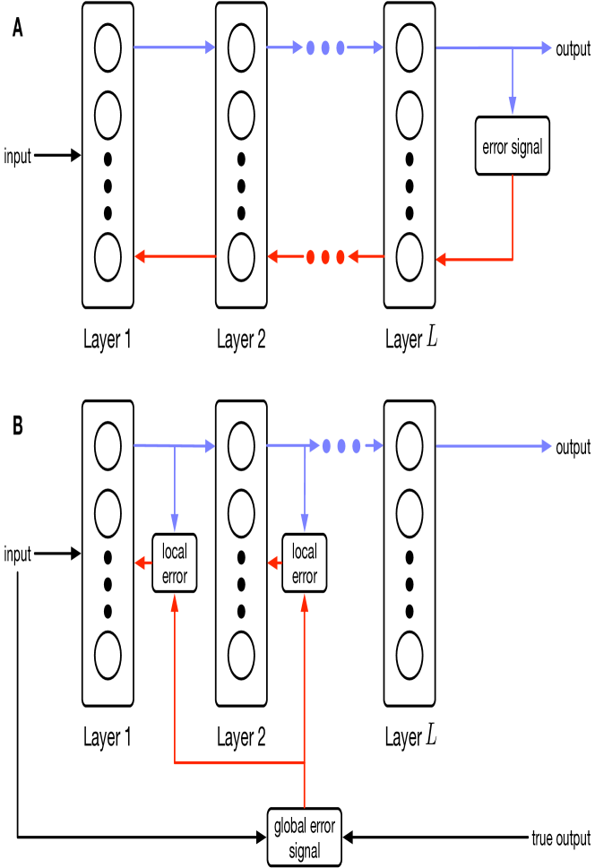
Figure 1: A. Sequential (explicit) error propagation requires precise information transfer backwards between layers. B. Parallel (implicit) error propagation uses only local information in combination with a global modulating signal. Biological rules of this form are known as three-factor learning rules (Frémaux and Gerstner, 2016).

In this work, we rely on recent advances in deep learning that train feedforward networks by balancing the information bottleneck (Ma, Lewis, and Kleijn, 2019). Unlike back-propagation, where an error signal computed at the end of the network is propagated to the front (see Fig. 1A), this method, called the Hilbert-Schmidt Independence Criterion (HSIC) bottleneck, applies the information bottleneck to each layer in the network independently. Layer-wise optimization is biologically plausible as shown in Fig. 1B.

Our contributions include:

1. We show that optimizing the HSIC bottleneck via gradient descent emits a three-factor learning rule (Frémaux and Gerstner, 2016) composed of a local Hebbian component and a global layer-wise modulating signal.

2. The HSIC bottleneck depends on a batch of samples, and this is reflected in our update rule. Unfortunately, the brain only sees a single sample at a time. We show that the local component only requires the current sample, and that the global component can be accurately computed by an auxiliary reservoir network. The reservoir acts as a working memory, and the effective “batch size” corresponds to its capacity.

3. We demonstrate the empirical performance of our update rule by comparing it against baselines on synthetic datasets as well as MNIST (LeCun, Cortes, and Burges, 1998).

4. To the best of our knowledge, our rule is the first to make a direct connection between working memory and synaptic updates. We explore this connection in some initial experiments on memory size and learning performance.

2 Related work

Several works have presented approximations to back-propagation. Variants of feedback alignment (Akrout et al., 2019; Liao, Leibo, and Poggio, 2016; Lillicrap et al., 2014) address the weight transport problem. Target propagation (Ahmad, van Gerven, and Ambrogioni, 2020) and equilibrium propagation (Scellier and Bengio, 2017) propose alternative mechanisms for propagating error. Yet, all these methods require separate inference (forward) and learning (backward) phases.

Layer-wise objectives (Belilovsky, Eickenberg, and Oyallon, 2019; Nøkland and Eidnes, 2019), like the one used in this work, offer an alternative that avoids the weight transport problem entirely. Moreover, our objective emits a biologically plausible three-factor learning rule which can be applied concurrently with inference. Pogodin and Latham (2020) draw similar intuition in their work on the plausible HSIC (pHSIC) learning rule. But in order to make experiments with the pHSIC computationally feasible, the authors used an approximation where the network “sees” 256 samples at once. In contrast, their proposed rule only receives information from two samples — the current one and the previous one. As shown in Fig. 2, we find this limited memory capacity reduces the effectiveness of weight updates. This motivates our work, in which we derive an alternate rule where only the global component depends on past samples (the local component only requires the current pre- and post-synaptic activity). Furthermore, we show that this global component can be computed using a reservoir network. This allows us to achieve performance much closer to back-propagation without compromising the biological plausibility of the rule.

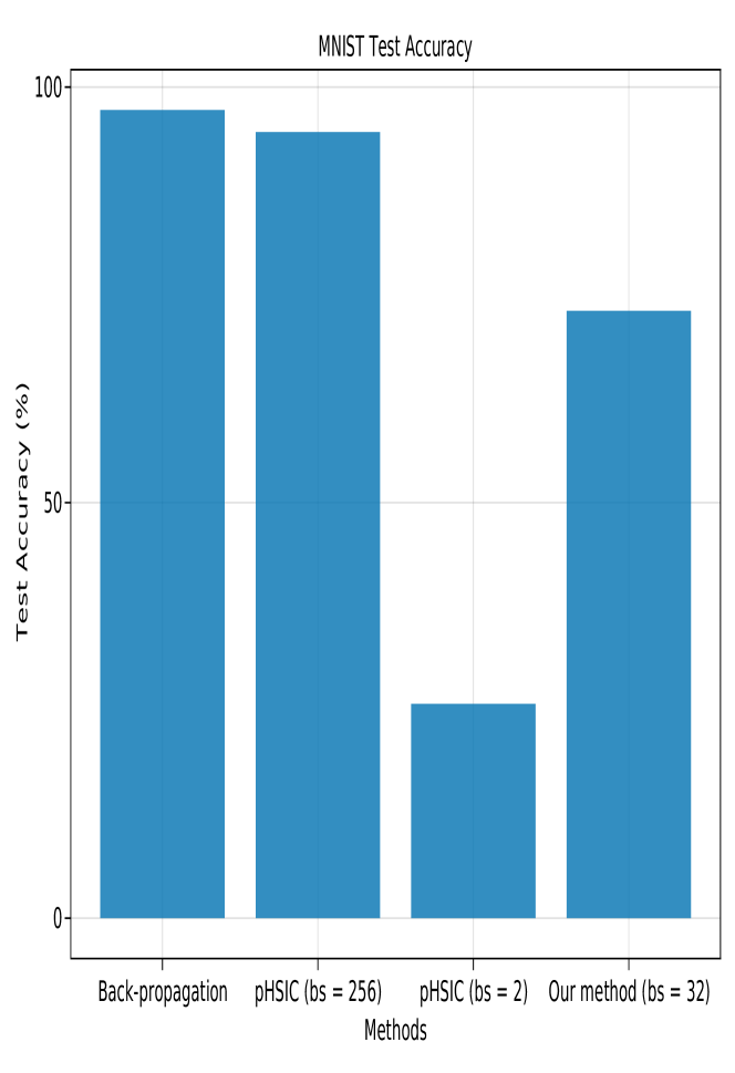
Figure 2: Final test accuracies on MNIST for various learning rules. pHSIC (plausible HSIC) is proposed in Pogodin and Latham (2020). “pHSIC (bs = 256)” is the accuracy reported in that work, and “pHSIC (bs = 2)” is the accuracy we obtain when applying the same rule with a reduced batch size. The degradation in performance is our motivation for deriving an alternate rule that effectively captures the batch size crucial to the HSIC bottleneck.

3 Notation

First, we will introduce the notation used in the paper.

• Vectors are indicated in bold and lower-case (e.g. $\mathbf{x}$).

• Matrices are indicated in bold and upper-case (e.g. $\mathbf{W}$).

• Superscripts refer to different layers of a feedforward network (e.g. $\mathbf{z}^{\ell}$ is the $\ell$-th layer).

• Subscripts refer to individual samples (e.g. $\mathbf{x}_{i}$ is the $i$-th sample).

• Brackets refer to elements within a matrix or vector (e.g. $[\mathbf{x}]_{i}$ is the $i$-th element of $\mathbf{x}$).

4 The information bottleneck

Given an input random variable, $X$, an output label random variable, $Y$, and hidden representation, $T$, the information bottleneck (IB) principle is described by

$$\min_{P_{T\mid X}}I(X;T)-\gamma I(T;Y)$$ (1)

where $I(X;Y)$ is the mutual information between two random variables. Intuitively, this expression adjusts $T$ to achieve a balance between information compression and output preservation.

Though computing the mutual information of two random variables requires knowledge of their distributions, Ma, Lewis, and Kleijn (2019) propose using the Hilbert-Schmidt Independence Criterion (HSIC) as a proxy for mutual information. Given a finite number of samples, $N$, a statistical estimator for the HSIC (Gretton et al., 2005) is

$$\mathrm{HSIC}(X,Y) =(N-1)^{-2}\mathrm{tr}(\mathbf{K_{X}}\mathbf{H}\mathbf{K_{Y}}\mathbf{H})$$ (2)

$$=\frac{1}{(N-1)^{2}}\sum_{p=1}^{N}\sum_{q=1}^{N}\bar{k}(\mathbf{x}_{p},\mathbf{x}_{q})\bar{k}(\mathbf{y}_{q},\mathbf{y}_{p})$$

$$[\mathbf{K_{X}}\mathbf{H}]_{pq} =\bar{k}(\mathbf{x}_{p},\mathbf{x}_{q})$$ (3)

$$=k(\mathbf{x}_{p},\mathbf{x}_{q})-\frac{1}{N}\sum_{n=1}^{N}k(\mathbf{x}_{p},\mathbf{x}_{n})$$

$$[\mathbf{K_{X}}]_{pq}=k(\mathbf{x}_{p},\mathbf{x}_{q})=\exp\left(-\frac{\|\mathbf{x}_{p}-\mathbf{x}_{q}\|^{2}}{\sigma^{2}}\right)$$ (4)

where Eq. 3 and 4 define the centered and uncentered kernel matrices, respectively.

Using these definitions Ma, Lewis, and Kleijn (2019) define the HSIC objective — a loss function for training feedforward neural networks by balancing the IB at each layer. Consider a feedforward neural network with $L$ layers where the output of layer $\ell$ is

$$\mathbf{z}^{\ell}=f(\mathbf{W}^{\ell}\mathbf{z}^{\ell-1})$$

We train the network to minimize

$$\mathcal{L}_{\mathrm{HSIC}}(X,Y,Z^{\ell}) =\mathrm{HSIC}(X,Z^{\ell})-\gamma\mathrm{HSIC}(Y,Z^{\ell})$$ (5)

$$\qquad\forall\ell\in\{1,\ldots,L\}$$

where $Z=\{Z^{\ell}\}_{\ell=1}^{L}$ are the output distributions at each hidden layer. Note that there is a separate objective for each layer. As a result, there is no explicit error propagation across layers, and the error propagation is implicit due to forward connectivity as shown in Fig. 1.

5 Deriving a biologically-plausible rule for the HSIC bottleneck

In this work, we seek to optimize Eq. 5 for a feedforward network of leaky integrate-and-fire (LIF) neurons. Given the membrane potentials, $\mathbf{u}^{\ell}$, for layer $\ell$, the dynamics are governed by

$$\tau_{\mathrm{ff}}\frac{\mathrm{d}\mathbf{u}^{\ell}}{\mathrm{d}t} =-\mathbf{u}+\mathbf{W^{\ell}}\mathbf{z}^{\ell-1}$$ (6)

$$\mathbf{z}^{\ell} =\tanh(\mathbf{u}^{\ell})+\zeta$$

where $\mathbf{z}^{\ell}$ is the output activity (firing rate) and $\zeta\sim\mathrm{Unif}(-0.05,0.05)$ emulates the firing rate noise.

We optimize $\mathcal{L}_{\mathrm{HSIC}}$ by taking the gradient with respect to $\mathbf{W}^{\ell}$ and applying gradient descent. Doing this, we obtain the following update rule:

$$\Delta[\mathbf{W}^{\ell}]_{ij} \propto\sum_{p,q=0}^{-(N-1)}\left[\bar{k}(\mathbf{x}_{p},\mathbf{x}_{q})-\gamma\bar{k}(\mathbf{y}_{p},\mathbf{y}_{q})\right]\bar{\alpha}_{ij}(\mathbf{z}_{p}^{\ell},\mathbf{z}_{q}^{\ell})$$ (7)

$$\bar{\alpha}_{ij}(\mathbf{z}_{p}^{\ell},\mathbf{z}_{q}^{\ell}) =\alpha_{ij}(\mathbf{z}_{p}^{\ell},\mathbf{z}_{q}^{\ell})-\frac{1}{N}\sum_{n=0}^{-(N-1)}\alpha_{ij}(\mathbf{z}_{p}^{\ell},\mathbf{z}_{n}^{\ell})$$

$$\alpha_{ij}(\mathbf{z}_{p}^{\ell},\mathbf{z}_{q}^{\ell}) =-\frac{k(\mathbf{z}_{p}^{\ell},\mathbf{z}_{q}^{\ell})}{\sigma^{2}}([\mathbf{z}_{p}^{\ell}]_{i}-[\mathbf{z}_{q}^{\ell}]_{i})$$

$$\qquad\left(\frac{\partial\mathbf{z}_{p}^{\ell}}{\partial[\mathbf{W}^{\ell}]_{ij}}-\frac{\partial\mathbf{z}_{q}^{\ell}}{\partial[\mathbf{W}^{\ell}]_{ij}}\right)$$

where $\alpha_{ij}$ is a Hebbian-like term between pre-synaptic neuron $j$ and post-synaptic neuron $i$. Note that the indices, $p$ and $q$, are from zero to $-(N-1)$ to indicate samples at previous time steps (i.e. $\mathbf{z}_{0}^{\ell}$ corresponds to the layer output now, $\mathbf{z}_{-1}^{\ell}$ corresponds to the layer output from the previously seen sample, etc.). We call $N$, the batch size in the deep learning, the effective batch size in our work. A full derivation of Eq. 7 can be found in the appendix. This rule is similar to the basic rule in Pogodin and Latham (2020), except that they replace $\bar{k}(\mathbf{x}_{p},\mathbf{x}_{q})$ with $\bar{k}(\mathbf{z}_{p},\mathbf{z}_{q})$ and do not use a centered kernel matrix.

Without modifications, Eq. 7 is not biologically plausible. $\alpha_{ij}(\mathbf{z}_{p}^{\ell},\mathbf{z}_{q}^{\ell})$ cannot be called Hebbian when $p$ and $q$ are not equal to zero, since it depends on non-local information from the past. We solve this by making a simplifying approximation. We assume that $\partial\mathbf{z}_{p}^{\ell}/\partial[\mathbf{W}^{\ell}]_{ij}=0$ when $p\neq 0$. In other words, the weights at the current time step do not affect past outputs. With this assumption, we find that $\alpha_{ij}(\mathbf{z}_{p}^{\ell},\mathbf{z}_{q}^{\ell})\neq 0$ if and only if $(p=0,q\neq 0)$ or $(p\neq 0,q=0)$. This gives us our final update rule:

$$\Delta[\mathbf{W}^{\ell}]_{ij} \propto\beta_{ij}\xi_{i}$$ (8)

$$\beta_{ij} =(1-([\mathbf{z}_{0}^{\ell}]_{i})^{2})[\mathbf{z}_{0}^{\ell-1}]_{j}$$

$$\xi_{i} =\sum_{p=0}^{-(N-1)}\left[\bar{k}(\mathbf{x}_{0},\mathbf{x}_{p})-\gamma\bar{k}(\mathbf{y}_{0},\mathbf{y}_{p})\right]\bar{\alpha}_{i}(\mathbf{z}_{p}^{\ell})$$

$$\bar{\alpha}_{i}(\mathbf{z}_{p}^{\ell}) =\alpha_{i}(\mathbf{z}_{p}^{\ell})-\frac{1}{N}\sum_{n=0}^{-(N-1)}\alpha_{i}(\mathbf{z}_{n}^{\ell})$$

$$\alpha_{i}(\mathbf{z}_{p}^{\ell}) =-\frac{2k(\mathbf{z}_{0}^{\ell},\mathbf{z}_{p}^{\ell})}{\sigma^{2}}(\mathbf{z}_{0}^{\ell}-\mathbf{z}_{p}^{\ell})$$

Details for deriving Eq. 8 from Eq. 7 are found in the appendix. Note that $\beta_{ij}$ is now a Hebbian term that only depends on the current pre- and post-synaptic activity. $\xi_{i}$ is a modulating term that adjusts the synaptic update layer-wise. This establishes a three-factor learning rule for Eq. 5. Yet, it is still not biologically plausible, since the global error, $\xi_{i}$, requires buffering layer activity over many samples. We discuss how to overcome this problem next.

5.1 Computing the modulating signal with a reservoir network

In order to compute $\xi_{i}$ in Eq. 8 biologically, we require a neural circuit capable of storing information for future use. Recurrent networks can provide such functionality, and Hoerzer, Legenstein, and Maass (2014) demonstrate how a reservoir network can be trained to compute complex signals using a binary teaching signal.

For each layer, we construct an auxiliary network of LIF neurons whose dynamics are governed by

$$\tau_{r}\frac{\mathrm{d}\mathbf{u}_{r}}{\mathrm{d}t} =-\mathbf{u}_{r}+\lambda\mathbf{W}_{r}\mathbf{r}+\mathbf{W}_{i}\mathbf{r}_{i}+\mathbf{W}_{\mathrm{fb}}\mathbf{r}_{o}$$ (9)

$$\mathbf{r} =\tanh(\mathbf{u}_{r})+\zeta_{r}$$

$$\mathbf{r}_{o} =\mathbf{W}_{o}\mathbf{u}_{r}+\zeta_{o}$$

where $\mathbf{u}_{r}$ are the recurrent neuron membrane potentials, $\mathbf{r}_{i}$ is the input signal activity, and $\mathbf{r}_{o}$ is the readout activity. $\zeta_{r}$ is the recurrent firing rate noise and $\zeta_{o}$ is the exploratory noise for the readout activity. $\lambda$ is a hyper-parameter that controls the chaos level of the recurrent population.

As stated in Hoerzer, Legenstein, and Maass (2014), we train the auxiliary network using a three-factor Hebbian learning rule shown below,

$$\Delta\mathbf{W}_{o} \propto M(\mathbf{r}_{o}-\bar{\mathbf{r}}_{o})\mathbf{r}^{\top}$$ (10)

$$M =\begin{cases}1&P>\bar{P}\\ 0&P\leq\bar{P}\end{cases}$$

$$P =-\|\mathbf{r}_{o}-\xi\|_{2}^{2}$$

where $\xi$ is the true global error signal in Eq. 8, $P$ is the negative mean-squared error of the current network output vs. the true signal, $M$ is a binary teaching signal derived from $P$, and $\bar{P}$, $\bar{\mathbf{r}}_{o}$ are low-pass filtered versions of $P$, $\mathbf{r}o$, respectively. The low-pass filter averages the signals over a moving window (based on the same function as Hoerzer, Legenstein, and Maass (2014)). Intuitively, this rule uses Hebbian updates to train the readout weights, but it gates the strength of the updates based on whether the network performance is improving or not.

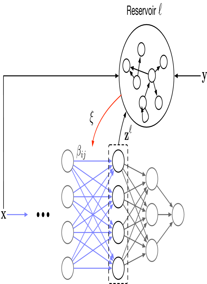
Figure 3: The overall network architecture. Each layer has a corresponding auxiliary reservoir network. The synaptic update, $\beta_{ij}$ in Eq. 8, is modulated by a layer-wise error signal, $\xi$, that is the readout from the reservoir.

Fig. 3 illustrates the full design of the proposed learning scheme. The reservoir serves as a working memory where the capacity of the memory determines the effective batch size. To the best of our knowledge, our rule is the first to modulate the Hebbian updates of a synapse based on past information stored in a working memory. Furthermore, having a controllable effective batch size means we can study the effect of memory capacity on the learning convergence. In particular, we can compare performance against the $N=2$ case which matches the biologically plausible variant of the prior work (Pogodin and Latham, 2020).

6 Experiments

We tested our design through a series of experiments on the reservoir individually and the full network on various synthetic and standard datasets. The code to reproduce each experiment is available at https://github.com/darsnack/biological-hsic along with instructions. Experiments were performed on a single node machine with a AMD Ryzen Threadripper 1950X 16-Core Processor and Nvidia Titan Xp GPU.

All data is normalized to $[0,1]$ to represent rate-encoded signals. Simulations use a time step of $1\text{\,}\mathrm{ms}$.

The learned output of the final layer via Eq. 5 is not necessarily one-hot like the true labels. This is because the HSIC objective only attempts to match the predicted output distribution and the true output distribution based on similarity between representations (this behavior is explained later in Fig. 8). Like Ma, Lewis, and Kleijn (2019), we use a linear readout layer trained for 1000 epochs with gradient descent to map between the HSIC-learned output and the label encoding. This is only required for our experiments. Biological circuitry would not require a specific label encoding.

6.1 Reservoir experiments

First, we verify the ability for the reservoir to reproduce the true signal $\xi$. We use a recurrent population of 2000 neurons with $\tau_{r}=$ $50\text{\,}\mathrm{ms}$ and $\lambda=1.2$ (based on recommendations in Hoerzer, Legenstein, and Maass (2014)). A hundred random input signals, $X\in\mathbb{R}^{100\times 100}$, $Y\in\mathbb{R}^{1\times 100}$, and $Z\in\mathbb{R}^{10\times 100}$, are drawn from $\mathrm{Unif}(0,1)$. We train the reservoir for $500\text{\,}\mathrm{s}$ to learn $\xi$ based on $X,Y,Z$, then stop the weight updates and test it for $100\text{\,}\mathrm{s}$. The following learning rate decay schedule is used

$$\eta(t)=\frac{\eta_{0}}{1+\frac{t}{\tau_{\text{decay}}}}$$

A complete list of parameters is in Table 1.

Parameter Name	Symbol	Value
LPF Time Constant	$\tau_{\mathrm{lpf}}$	$5\text{\,}\mathrm{ms}$
Sample Time Constant	$\Delta t_{\text{sample}}$	$50\text{\,}\mathrm{ms}$
Hidden Firing Noise	$\zeta_{r}$	$5\text{\times}{10}^{-6}$
Readout Firing Noise	$\zeta_{o}$	$1\text{\times}{10}^{-2}$
Effective Batch Size	$N$	$6$
HSIC Balance Parameter	$\gamma$	$2$
Learning Rate	$\eta_{0}$	$1\text{\times}{10}^{-4}$
Learning Rate Decay	$\tau_{\text{decay}}$	$20\text{\,}\mathrm{s}$

Table 1: Reservoir experiment parameters.

The results can be seen in Fig. 4 which shows the reservoir output for the first element of the output signal. Prior to training, the output is pure noise, but it begins to match the true signal quickly after training begins. Even when the training is stopped, the reservoir continues to produce the correct output for the full testing period.

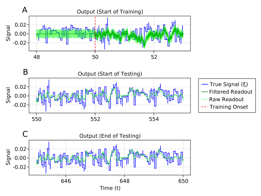
Figure 4: The reservoir output when learning $\xi$ in Eq. 8. A. The output at the right before and after the start of training. When the training begins, the readout quickly begins to match the true signal. B. The output at the start of testing. Even without the feedback from the learning rule, the output matches the true signal. C. The output at the end of testing ($100\text{\,}\mathrm{s}$ later) continues to maintain the correct behavior.

6.2 Small dataset experiments

In order to demonstrate that a reservoir readout can effectively modulate learning for a complete network, we perform a series of small-scale experiments. These experiments use simple synthetic datasets through which we can gain an intuitive understanding of the learning behavior. In addition to the parameters listed in Table 1, Table 2 contains shared parameters for all small-scale experiments.

Parameter Name	Symbol	Value
Network LIF Time Constant	$\tau_{\mathrm{ff}}$	$5\text{\,}\mathrm{ms}$
Reservoir Chaos Level	$\lambda$	$1.7$
Hidden Firing Noise	$\zeta_{r}$	$5\text{\times}{10}^{-2}$
Readout Firing Noise	$\zeta_{o}$	$2.5\text{\times}{10}^{-1}$
# of Hidden Neurons	$N_{\text{hidden}}$	$1000$
Effective Batch Size	$N$	$10$
Network Learning Rate	$\eta_{0}$	$5\text{\times}{10}^{-3}$
Network Learning Rate Decay	$\tau_{\text{decay}}$	$50\text{\,}\mathrm{s}$

Table 2: Small-scale experiment parameters.

First, we test a single layer perceptron on a linear binary classification task. We separated 100 uniformly sampled points from $[-1,1]\times[-1,1]$ using a line as shown in Fig. 5A. We pre-train the reservoir network for $550\text{\,}\mathrm{s}$ with $\gamma=5$, then we perform 50 epochs of training on the dataset. The network reached a final classification accuracy of 94%. Furthermore, the ratio of the learned weights converges towards the ratio of the true coefficients of the linear boundary.

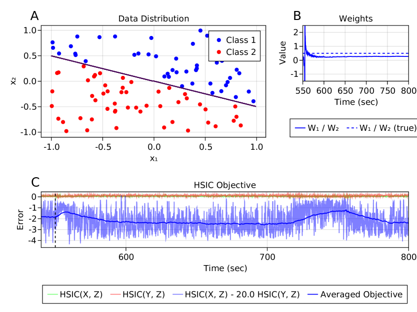
Figure 5: The results from training a single layer perceptron on a linear binary classification task. A. An example sample set from the synthetic distribution. B. The ratio of the two weights in the model converges the true ratio. C. The HSIC objective converges due to the learning rule. The final test accuracy is 94%.

Next, we test a multilayer perceptron (MLP) network with an auxiliary reservoir in place for each layer. A synthetic 2D binary classification dataset is generated by sampling 100 random points in $[-1,1]\times[-1,1]$ uniformly, then separating the points by the decision boundary $x_{2}=\tanh(3x_{1})$. An example generated dataset is shown in Fig. 6A. The MLP architecture is two layers of size two and one, respectively. We warm-up and pre-train the reservoir network for $550\text{\,}\mathrm{s}$ with $\gamma=20$, then we run 50 epochs of training with our rule. On testing, the network achieves 98% accuracy.

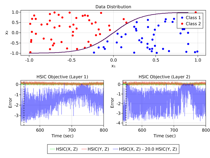
Figure 6: The results from training a two-layer MLP on a synthetic binary classification dataset. A. An example sample set from the synthetic distribution. B. The HSIC objective (Eq. 5) for each layer. The plain objective value is very noisy due to the noise in the neuron firing rate. Despite this noise, the network converges and reaches 98% accuracy.

In both small experiments, there is a noticeable oscillation in the objective value during training. We attribute this instability to the output of the reservoir falling out of phase with the true signal before returning in-phase. This behavior was noted in Hoerzer, Legenstein, and Maass (2014), and it is periodic. In our experiments, we disable weight updates to the reservoir to demonstrate the ability for the full framework to learn even with an imperfect modulating signal. In practice, the reservoir can be continuously updated, which will eliminate the phase shift (Hoerzer, Legenstein, and Maass, 2014).

6.3 Large dataset experiments

Finally, we test our rule on MNIST with an MLP against a back-propagation baseline. The architecture used for all learning frameworks is a $784\Rightarrow 64\Rightarrow 32\Rightarrow 10\Rightarrow 10$ network. The back-propagation baseline uses ReLU activation and artificial neurons like those typically used in deep learning. Our method uses LIF neurons as described in Sec. 5.

Since our learning rule is designed to process single samples at a time, we must iterate and train on MNIST a single sample at a time. This becomes computationally infeasible due to the large dataset size. In order to make the experiments tractable, we do not simulate the reservoir neurons. Having already established their ability to capture the global signal, $\xi$, correctly, we compute the signal analytically. Furthermore, we obtain a subset of MNIST by sampling 50% of the points in the training data via stratified sampling. We retain the complete test data for reporting final accuracy. The back-propagation network is trained with a batch size of 32, and our rule uses an effective batch size of 32. The networks are all trained for 75 epochs, and each sample is presented for $20\text{\,}\mathrm{ms}$. The HSIC balance parameter, $\gamma$, is set to 50, 100, 200, and 500, for each layer, respectively. We use a momentum optimizer (with momentum, $\rho=0.9$) purely to speed up convergence and make the experiment tractable. The learning rate starts at $5\text{\times}{10}^{-2}$ for 20 epochs, drops to $5\text{\times}{10}^{-3}$ for 30 epochs, and finally $1\text{\times}{10}^{-3}$ for the remaining training time. The remaining parameters match the previous experiments.

We performed four trials to account for random seeds and show the average test accuracy across trials in Fig. 7. Despite failing to match the same accuracy as back-propagation, our method is able to improve and learn the dataset. After 75 epochs, our objective value continued to decrease but at a diminished rate. We expect that the gap between our method and back-propagation would be smaller with more epochs of training; however, our goal is not to establish a state-of-the-art method for training. Instead, we are demonstrating a biologically-plausible rule that can scale up to larger datasets.

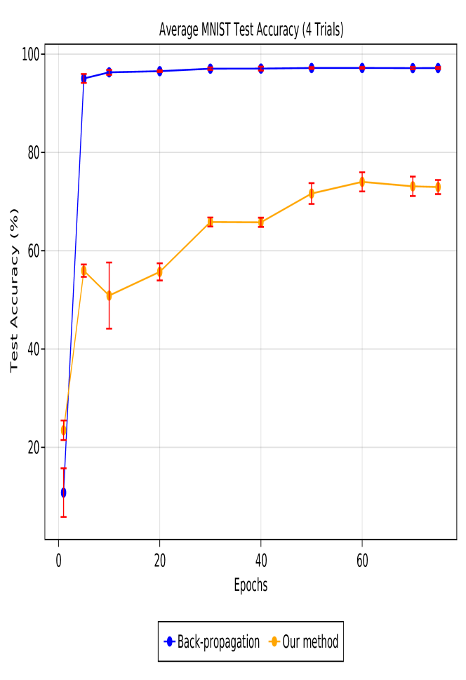
Figure 7: Average test accuracy over four independent trials on MNIST for back-propagation and our method. The red error bars indicate the standard deviation across trials. Our method improves in accuracy as training proceeds, but convergence quickly slows down. We expect the gap in performance to close with more epochs but running for many epochs was computationally intractable for this work.

In addition to examining the test accuracy, we show the average predicted output per class from one the trials in Fig. 8. We see that the predictions do not match a one-hot vector, but each label is assigned a unique binary “code word.”

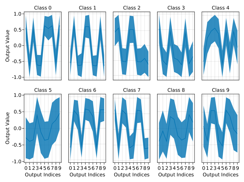
Figure 8: The average predicted output across all test samples on MNIST separated by true label (the shaded region indicates the standard deviation across test samples). Each subplot corresponds to a single true label, and the solid line is the mean output for the final HSIC-trained layer. As expected, the output is not one-hot, but the network does tend to learn a unique binary “code word” for each class.

Note that we repeat these experiments with pHSIC (batch size = 2) and LIF neurons to produce the result in Fig. 2.

In order to demonstrate that our rule can scale up to larger datasets with sufficient iterations, we create a subset of MNIST by only selecting samples for the digits 0, 1, 2, and 4. We repeat our experiment on this subset of data. The results are shown in Fig. 9. With a slightly smaller, but still complex dataset, our method achieves comparable performance to back-propagation.

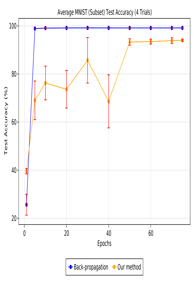
Figure 9: The average test accuracy across 4 trials on a subset of MNIST (only digits 0, 1, 2, and 4). Our method (94% accuracy) achieves comparable performance to back-propagation.

6.4 Effects of memory capacity

One of the novel features of our rule is the ability to control the memory capacity of the update. To explore this parameter, we repeat the same MNIST experiments as before for various effective batch sizes and number of epochs of training. The results are shown in Fig. 10. The normalized final test accuracy is much lower for small batch sizes independent of the number of training epochs. This is because for a given random variable, $X\in\mathbb{R}^{n}$, the kernel matrix, $\mathbf{K}_{X}$, is the basis for an estimate of how samples of $X$ are distributed in $\mathbb{R}^{n}$. When the effective batch size is small, this estimate is poor and provides an erroneous signal for modulating the weight updates. In particular, note that $\alpha_{i}(\mathbf{z}_{p}^{\ell})$ in Eq. 8 has an anti-Hebbian behavior — it tends to drive $\mathbf{z}_{0}^{\ell}$ and $\mathbf{z}_{p}^{\ell}$ (the latent representation for layer $\ell$) apart. This signal is flipped whenever $\bar{k}(\mathbf{y}_{0},\mathbf{y}_{p})$ is large. In other words, if $\mathbf{y}_{0}$ is more similar to $\mathbf{y}_{p}$ than it is to other samples, the latent representations are driven towards each other. When the batch size is small, $\mathbf{K}_{Y}$ rarely contains samples of the same label, so the rule tends to over-drive the latent representations apart.

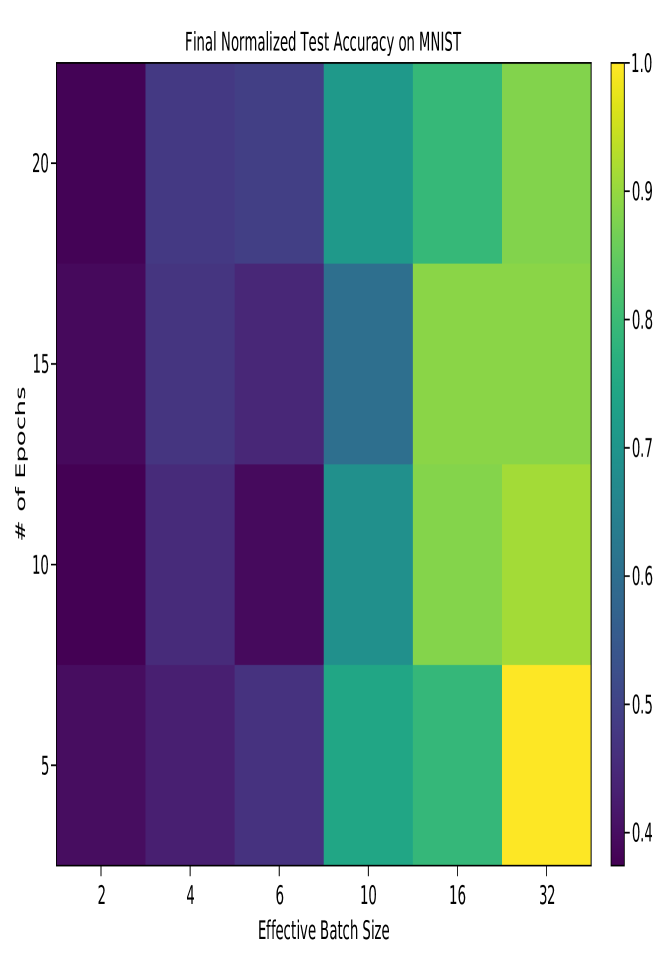
Figure 10: The final normalized test accuracy on MNIST for varying number of epochs and effective batch sizes. We see that the accuracy is degraded for small batch sizes independent of the number of epochs.

7 Discussion

In this work, we proposed a three-factor learning rule for training feedforward networks based on the information bottleneck principle. The rule is biologically plausible, and we are able to scale up to reasonable performance on MNIST without compromise. We do this by factoring our weight update into a local component and global component. The local component depends only on the current synaptic activity, so it can be implemented via Hebbian learning. In contrast to prior work, our global component uses information across many samples seen over time. We show that this content can be stored in an auxiliary reservoir network, and the readout of the reservoir can be used to modulate the local weight updates. To the best of our knowledge, this is the first biological learning rule to tightly couple the synaptic updates with a working memory capacity. We verified the efficacy of our rule on synthetic datasets and MNIST, and we explored the effect of the size of the working memory capacity on the learning performance.

Even though our rule does perform reasonably well, there is room for improvement. The rule performs best when it is able to distinguish between different high dimensional inputs. The resolution at which it separates inputs is controlled by the parameter, $\sigma$, in the kernel function (Eq. 4). The use of a fixed $\sigma$ is partly responsible for the slow down in convergence in Fig. 7. In Ma, Lewis, and Kleijn (2019), the authors propose using multiple networks trained with the different values of $\sigma$ and averaging the output across networks. This allows the overall network to separate the data at different resolutions. Future work can consider a population of networks with varying $\sigma$ to achieve the same effect. Alternatively, the lower hierarchies of the visual cortex have built-in pre-processing at varying spatial resolutions (e.g. Gabor filters). We could consider adding a series of filters before the network and pass the concatenated output to the network. Addressing the resolution issue will be important for improving the speed and scalability of the learning method.

Additionally, our rule is strongly supervised. While the mechanism for synaptic updates is biologically plausible, the overall learning paradigm is not. Note that the purpose of the label information in the global signal is to indicate whether the output for the current sample should be the same or different from previous samples. In other words, it might be possible to replace the term $\bar{k}(\mathbf{y}_{0},\mathbf{y}_{p})$ in Eq. 8 with a binary teaching signal. This would allow the rule to operate under weak supervision.

Most importantly, while our rule is certainly biologically plausible, it remains to be seen if it is an accurate model for circuitry in the brain. Since rules based on the information bottleneck are relatively new, the corresponding experimental evidence must still be obtained. Yet, we note that our auxiliary reservoir serves a similar role to the “blackboard” circuit proposed in Mumford (1991). This circuit, present in the thalamus, receives projected connections from the visual cortex, similar to how each layer projects its output onto the reservoir. Furthermore, Mumford suggests that this circuit acts as a temporal buffer and sends signals that capture information over longer timescales back to the cortex like our reservoir.

So, while it is uncertain whether our exact rule and memory circuit are present in biology, we suggest that an in-depth exploration of memory-modulated learning rules is necessary. We hope this work will be an important step in that direction.

Appendix A Derivation of learning rule

Below is a complete derivation of our update rule. First, we find the derivative of $\mathcal{L}_{\mathrm{HSIC}}$ (Eq. 5) with respect to the layer weight, $\mathbf{W}^{\ell}$. Then, we show the assumptions necessary to make this update biologically plausible.

First, we re-index the summation in Eq. 2 such that samples $\{1,2,\ldots,N\}$ are now samples $\{0,-1,\ldots,-(N-1)\}$ over time.

$$\mathrm{HSIC}(X,Y)=\frac{1}{(N-1)^{2}}\sum_{p,q=0}^{-(N-1)}\bar{k}(\mathbf{x}_{p},\mathbf{x}_{q})\bar{k}(\mathbf{y}_{q},\mathbf{y}_{p})$$ (11)

In other words, the first sample in the batch is the current sample, and the last sample in the batch is the one presented $N-1$ samples ago. Now, taking the derivative of Eq. 5 with respect to $[\mathbf{W}]_{ij}^{\ell}$:

$$\>\quad\frac{\partial\mathcal{L}_{\mathrm{HSIC}}(X,Y,Z^{\ell})}{\partial[\mathbf{W}]_{ij}^{\ell}}$$ (12)

$$=\frac{\partial}{\partial[\mathbf{W}]_{ij}^{\ell}}\Big{[}\mathrm{HSIC}(X,Z^{\ell})-\lambda\mathrm{HSIC}(Y,Z^{\ell})\Big{]}$$

$$=\frac{\partial}{\partial[\mathbf{W}]_{ij}^{\ell}}\left[\frac{1}{(N-1)^{2}}\sum_{p,q=0}^{-(N-1)}\bar{k}(\mathbf{z}_{p}^{\ell},\mathbf{z}_{q}^{\ell})\bar{k}(\mathbf{x}_{q},\mathbf{x}_{p})\right.$$

$$\qquad\qquad\qquad\qquad\qquad\qquad-\gamma\bar{k}(\mathbf{z}_{p}^{\ell},\mathbf{z}_{q}^{\ell})\bar{k}(\mathbf{y}_{q},\mathbf{y}_{p})\Bigg{]}$$

$$=\frac{1}{(N-1)^{2}}\sum_{p,q=0}^{-(N-1)}\Big{[}\bar{k}(\mathbf{x}_{q},\mathbf{x}_{p})-\gamma\bar{k}(\mathbf{y}_{q},\mathbf{y}_{p})\Big{]}\frac{\partial\bar{k}(\mathbf{z}_{p}^{\ell},\mathbf{z}_{q}^{\ell})}{\partial[\mathbf{W}]_{ij}^{\ell}}$$

Focusing on the derivative of $\bar{k}(\mathbf{z}_{p}^{\ell},\mathbf{z}_{q}^{\ell})$,

$$\frac{\partial\bar{k}(\mathbf{z}_{p}^{\ell},\mathbf{z}_{q}^{\ell})}{\partial[\mathbf{W}]_{ij}^{\ell}} =\frac{\partial}{\partial[\mathbf{W}]_{ij}^{\ell}}\left[k(\mathbf{z}_{p}^{\ell},\mathbf{z}_{q}^{\ell})-\frac{1}{N}\sum_{n=0}^{-(N-1)}k(\mathbf{z}_{p}^{\ell},\mathbf{z}_{n}^{\ell})\right]$$

$$=\frac{\partial k(\mathbf{z}_{p}^{\ell},\mathbf{z}_{q}^{\ell})}{\partial[\mathbf{W}]_{ij}^{\ell}}-\frac{1}{N}\sum_{n=0}^{-(N-1)}\frac{\partial k(\mathbf{z}_{p}^{\ell},\mathbf{z}_{n}^{\ell})}{\partial[\mathbf{W}]_{ij}^{\ell}}$$

And finally,

$$\frac{\partial k(\mathbf{z}_{p}^{\ell},\mathbf{z}_{q}^{\ell})}{\partial[\mathbf{W}]_{ij}^{\ell}} =\frac{\partial}{\partial[\mathbf{W}]_{ij}^{\ell}}\left[\exp\left(-\frac{\|\mathbf{z}_{p}^{\ell}-\mathbf{z}_{q}^{\ell}\|^{2}}{2\sigma^{2}}\right)\right]$$

$$=-\frac{k(\mathbf{z}_{p}^{\ell},\mathbf{z}_{q}^{\ell})}{2\sigma^{2}}\left(\frac{\partial\|\mathbf{z}_{p}^{\ell}-\mathbf{z}_{q}^{\ell}\|^{2}}{\partial[\mathbf{W}]_{ij}^{\ell}}\right)$$

$$=-\frac{k(\mathbf{z}_{p}^{\ell},\mathbf{z}_{q}^{\ell})([\mathbf{z}_{p}]_{i}^{\ell}-[\mathbf{z}_{q}]_{i}^{\ell})}{\sigma^{2}}$$

$$\quad\left(\frac{\partial\mathbf{z}_{p}^{\ell}}{\partial[\mathbf{W}]_{ij}^{\ell}}-\frac{\partial\mathbf{z}_{q}^{\ell}}{\partial[\mathbf{W}]_{ij}^{\ell}}\right)$$

This gives us the update rule form in Eq. 7. The term $\frac{\partial\mathbf{z}_{p}^{\ell}}{\partial[\mathbf{W}]_{ij}^{\ell}}-\frac{\partial\mathbf{z}_{q}^{\ell}}{\partial[\mathbf{W}]_{ij}^{\ell}}$ is the local component, while the rest can be globally computer per layer. But this rule is not biologically plausible, since the local indices $p$ and $q$ sample neuron firing rates from past time steps.

We make the assumption that $\frac{\partial\mathbf{z}_{p}^{\ell}}{\partial[\mathbf{W}]{ij}^{\ell}}=0$ when $p\neq 0$ (similarly when $q\neq 0$). In other words, the past output does not depend on the current weights. With this assumption, we note that

$$\frac{\partial\mathbf{z}_{p}^{\ell}}{\partial[\mathbf{W}]_{ij}^{\ell}}\begin{cases}(1-[\mathbf{z}_{0}^{\ell}]_{i})^{2}[\mathbf{z}_{0}^{\ell-1}]_{j}&p=0\\ 0&p\neq 0\end{cases}$$

Additionally, when both $(p=0,q=0)$,

$$\frac{\partial\mathbf{z}_{p}^{\ell}}{\partial[\mathbf{W}]_{ij}^{\ell}}-\frac{\partial\mathbf{z}_{q}^{\ell}}{\partial[\mathbf{W}]_{ij}^{\ell}}=0$$

Thus, we find that each term in the summation in Eq. 12 is non-zero only when $(p\neq 0,q=0)$ and $(p=0,q\neq 0)$. Furthermore, due to the symmetry of the terms, we can reduce the double-summation into twice times a single-summation. This gives us our final form

$$\Delta[\mathbf{W}^{\ell}]_{ij} \propto\beta_{ij}\xi_{i}$$

$$\beta_{ij} =(1-([\mathbf{z}_{0}^{\ell}]_{i})^{2})[\mathbf{z}_{0}^{\ell-1}]_{j}$$

$$\xi_{i} =\sum_{p=0}^{-(N-1)}\left[\bar{k}(\mathbf{x}_{0},\mathbf{x}_{p})-\gamma\bar{k}(\mathbf{y}_{0},\mathbf{y}_{p})\right]\bar{\alpha}_{i}(\mathbf{z}_{p}^{\ell})$$

$$\bar{\alpha}_{i}(\mathbf{z}_{p}^{\ell}) =\alpha_{i}(\mathbf{z}_{p}^{\ell})-\frac{1}{N}\sum_{n=0}^{-(N-1)}\alpha_{i}(\mathbf{z}_{n}^{\ell})$$

$$\alpha_{i}(\mathbf{z}_{p}^{\ell}) =-\frac{2k(\mathbf{z}_{0}^{\ell},\mathbf{z}_{p}^{\ell})}{\sigma^{2}}(\mathbf{z}_{0}^{\ell}-\mathbf{z}_{p}^{\ell})$$

where $\beta_{ij}=\frac{\partial\mathbf{z}_{0}^{\ell}}{\partial[\mathbf{W}]_{ij}^{\ell}}$ is factored out of the summation since it no longer depends on $p$. This results in a local component, $\beta_{ij}$, that can be computed using only the current pre- and post-synaptic activity. The global component, $\xi$, requires memory, so we use an auxiliary network to compute it.

Appendix B Reservoir network details

Here we explain the low-pass filtering (LPF) details not covered by the behavior described in Sec. 5, Eq. 9. As part of the learning rule in Eq. 10, the readout and error signals are low-pass filtered according to

$$\bar{f}(t)=\left(1-\frac{\Delta t}{\tau_{\mathrm{lpf}}}\right)\bar{f}(t-\Delta t)+\frac{\Delta t}{\tau_{\mathrm{lpf}}}f(t)$$ (13)

where $\Delta t$ is the simulation time step. This is the same filtering technique presented in Hoerzer, Legenstein, and Maass (2014).

References

- Ahmad, van Gerven, and Ambrogioni (2020) Ahmad, N.; van Gerven, M.; and Ambrogioni, L. 2020. GAIT-Prop: A Biologically Plausible Learning Rule Derived from Backpropagation of Error. In Advances in Neural Information Processing Systems, volume 33, 10913–10923. Curran Associates, Inc.
- Akrout et al. (2019) Akrout, M.; Wilson, C.; Humphreys, P.; Lillicrap, T.; and Tweed, D. B. 2019. Deep Learning without Weight Transport. In Advances in Neural Information Processing Systems, volume 31, 9. Curran Associates, Inc.
- Balduzzi, Vanchinathan, and Buhmann (2015) Balduzzi, D.; Vanchinathan, H.; and Buhmann, J. 2015. Kickback Cuts Backprop’s Red-Tape: Biologically Plausible Credit Assignment in Neural Networks. In Proceedings of the Twenty-Ninth AAAI Conference on Artificial Intelligence, 7.
- Belilovsky, Eickenberg, and Oyallon (2019) Belilovsky, E.; Eickenberg, M.; and Oyallon, E. 2019. Greedy Layerwise Learning Can Scale to ImageNet. In Proceedings of Machine Learning Research, volume 97, 583–593. PMLR.
- Frémaux and Gerstner (2016) Frémaux, N.; and Gerstner, W. 2016. Neuromodulated Spike-Timing-Dependent Plasticity, and Theory of Three-Factor Learning Rules. Frontiers in Neural Circuits, 9.
- Gretton et al. (2005) Gretton, A.; Bousquet, O.; Smola, A.; and Schölkopf, B. 2005. Measuring Statistical Dependence with Hilbert-Schmidt Norms. In Hutchison, D.; Kanade, T.; Kittler, J.; Kleinberg, J. M.; Mattern, F.; Mitchell, J. C.; Naor, M.; Nierstrasz, O.; Pandu Rangan, C.; Steffen, B.; Sudan, M.; Terzopoulos, D.; Tygar, D.; Vardi, M. Y.; Weikum, G.; Jain, S.; Simon, H. U.; and Tomita, E., eds., Algorithmic Learning Theory, volume 3734, 63–77. Berlin, Heidelberg: Springer Berlin Heidelberg. ISBN 978-3-540-29242-5 978-3-540-31696-1.
- Hoerzer, Legenstein, and Maass (2014) Hoerzer, G. M.; Legenstein, R.; and Maass, W. 2014. Emergence of Complex Computational Structures From Chaotic Neural Networks Through Reward-Modulated Hebbian Learning. Cerebral Cortex, 24(3): 677–690.
- LeCun, Cortes, and Burges (1998) LeCun, Y.; Cortes, C.; and Burges, C. J. 1998. MNIST Handwritten Digit Database.
- Liao, Leibo, and Poggio (2016) Liao, Q.; Leibo, J. Z.; and Poggio, T. 2016. How Important Is Weight Symmetry in Backpropagation? In Proceedings of the Thirtieth AAAI Conference on Artificial Intelligence, 8. North America.
- Lillicrap et al. (2014) Lillicrap, T. P.; Cownden, D.; Tweed, D. B.; and Akerman, C. J. 2014. Random Feedback Weights Support Learning in Deep Neural Networks. arXiv:1411.0247 [cs, q-bio].
- Lillicrap et al. (2020) Lillicrap, T. P.; Santoro, A.; Marris, L.; Akerman, C. J.; and Hinton, G. 2020. Backpropagation and the Brain. Nature Reviews Neuroscience, 21(6): 335–346.
- Ma, Lewis, and Kleijn (2019) Ma, W.-D. K.; Lewis, J. P.; and Kleijn, W. B. 2019. The HSIC Bottleneck: Deep Learning without Back-Propagation. arXiv:1908.01580 [cs, stat].
- Mumford (1991) Mumford, D. 1991. On the Computational Architecture of the Neocortex: I. The Role of the Thalamo-Cortical Loop. Biological Cybernetics, 65(2): 135–145.
- Nøkland and Eidnes (2019) Nøkland, A.; and Eidnes, L. H. 2019. Training Neural Networks with Local Error Signals. In Proceedings of Machine Learning Research, volume 97, 4839–4850. PMLR.
- Pogodin and Latham (2020) Pogodin, R.; and Latham, P. E. 2020. Kernelized Information Bottleneck Leads to Biologically Plausible 3-Factor Hebbian Learning in Deep Networks. In Advances in Neural Information Processing Systems, volume 33, 12. Curran Associates, Inc.
- Scellier and Bengio (2017) Scellier, B.; and Bengio, Y. 2017. Equilibrium Propagation: Bridging the Gap between Energy-Based Models and Backpropagation. Frontiers in Computational Neuroscience, 11: 24.