An efficient IMEX-DG solver for the compressible Navier-Stokes equations for non-ideal gases

Giuseppe Orlando(1)
Paolo Francesco Barbante(1), Luca Bonaventura(1)
Abstract

We propose an efficient, accurate and robust IMEX solver for the compressible Navier-Stokes equation describing non-ideal gases with general equations of state. The method, which is based on an hlimit-fromh-adaptive Discontinuos Galerkin spatial discretization and on an Additive Runge Kutta IMEX method for time discretization, is tailored for low Mach number applications and allows to simulate low Mach regimes at a significantly reduced computational cost, while maintaining full second order accuracy also for higher Mach number regimes. The method has been implemented in the framework of the deal.II numerical library, whose adaptive mesh refinement capabilities are employed to enhance efficiency. Refinement indicators appropriate for real gas phenomena have been introduced. A number of numerical experiments on classical benchmarks for compressible flows and their extension to real gases demonstrate the properties of the proposed method.

(1) MOX, Dipartimento di Matematica, Politecnico di Milano
Piazza Leonardo da Vinci 32, 20133 Milano, Italy
giuseppe.orlando@polimi.it, luca.bonaventura@polimi.it, paolo.barbante@polimi.it

Keywords: Navier-Stokes equations, compressible flows, Discontinuous Galerkin methods, implicit methods, ESDIRK methods.

AMS Subject Classification: 65M12, 65M50, 65M60, 65Y05, 76N06

1 Introduction

The efficient numerical solution of the compressible Navier-Stokes equations poses several major computational challenges. In particular, for flow regimes characterized by low Mach number and moderate Reynolds number values, severe time step restrictions may be required by standard explicit time discretization methods. The use of implicit and semi-implicit methods has a long tradition in low Mach number flows, see for example the seminal papers [12, 13, 45], as well as many other contributions in the literature on numerical weather prediction, see e.g. [6, 21, 23, 24, 33, 44, 46, 52] and the reviews in [49, 8]. Other contributions have been proposed in the literature on more classical computational fluid dynamics, see e.g. [5, 4, 10, 11, 14, 38, 51]. Many of these contributions focus exclusively on the equations of motion of an ideal gas and their extension to real gases is not necessarily straightforward. Stability concerns are even more critical in these particular regimes for spatial discretizations based on the Discontinuous Galerkin (DG) method (see e.g. [22, 30] for a general presentation of this method), which is the spatial discretization used in many of the above referenced papers.

In this work, we seek to combine an accurate and flexible discontinuous DG space discretization with a second order implicit-explicit (IMEX) time discretization, see e.g. [31, 42, 9], to obtain an efficient method for compressible flow of real gases at low to moderate Mach numbers. Our goal is to derive a method that can then be easily extended to handle multiphase compressible flows, where a number of coupling and forcing terms arise that cannot be dealt with efficiently by straightforward application of conventional solvers. We extend to second order in time the approach of [12, 14], coupling implicitly the energy equation to the momentum equation, while treating the continuity equation in an explicit fashion. Our treatment also provides an outline of how a generic IMEX method based on a Diagonally Implicit Runge Kutta can be extended along the same lines. Notice that, with respect to the IMEX approach proposed for the Euler equations in [54], the technique presented here does not require to introduce reference solutions, does not introduce inconsistencies in the splitting with respect to a reference solution and only requires the solution of linear system of a size equal to that of the number of discrete degrees of freedom needed to describe a scalar variable, as in [14]. A conceptually similar approach has been used in [33, 46] for the discretization employed in the IFS-FVM atmospheric model. In order to obtain a formulation that is efficient also in presence of non negligible viscous terms, we resort to an operator splitting approach, see e.g. [36]. More specifically, as commonly done in numerical models for atmospheric physics, we split the hyperbolic part of the problem, which is treated by an IMEX extension of the method proposed in [14], from the diffusive terms, which are treated implicitly. Second order accuracy can then be obtained by the Strang splitting approach [36, 50].

For the spatial discretization, we rely on the DG approach implemented in the numerical library deal.II [2], which is a very convenient environment to develop a reliable and easily accessible tool for large scale industrial applications. This software also provides hlimit-fromh-refinement capabilities that are exploited by the proposed method. For the specific case of real gases, physically based refinement criteria have been proposed and tested, which allow to track accurately convection phenomena also for more general equations of state. The numerical experiments reported below show the ability of the proposed scheme and of its adaptive implementation to perform accurate simulations in a range of different settings appropriate to describe non-ideal gas dynamics.

The model equations and their non-dimensional formulation are reviewed in Section 2. The time discretization approach is outlined and discussed in Section 4. The spatial discretization is presented in Section 5. Some implementation issues are described in Section 6, while the validation of the proposed method and its application to a number of significant benchmarks is reported in Section 7. Some conclusions and perspectives for future work are presented in Section 8.

2 The compressible Navier-Stokes equations

Let Ωd,2d3formulae-sequenceΩsuperscript𝑑2𝑑3\Omega\subset\mathbb{R}^{d},2\leq d\leq 3 be a connected open bounded set with a sufficiently smooth boundary ΩΩ\partial\Omega and denote by 𝐱𝐱\mathbf{x} the spatial coordinates and by t𝑡t the temporal coordinate. We consider the classical unsteady compressible Navier-Stokes equations, written in flux form as:

ρt+(ρ𝐮)\displaystyle\frac{\partial\rho}{\partial t}+\operatorname{\nabla\cdot}\left(\rho\mathbf{u}\right) =\displaystyle= 00\displaystyle 0
(ρ𝐮)t+(ρ𝐮𝐮)+p\displaystyle\frac{\partial(\rho\mathbf{u})}{\partial t}+\operatorname{\nabla\cdot}\left(\rho\mathbf{u}\otimes\mathbf{u}\right)+\nabla p =\displaystyle= 𝝉+ρ𝐟\displaystyle\operatorname{\nabla\cdot}\boldsymbol{\tau}+\rho\mathbf{f} (1)
(ρE)t+[(ρE+p)𝐮]\displaystyle\frac{\partial(\rho E)}{\partial t}+\operatorname{\nabla\cdot}\left[(\rho E+p)\mathbf{u}\right] =\displaystyle= (𝝉𝐮𝐪)+ρ𝐟𝐮\displaystyle\operatorname{\nabla\cdot}(\boldsymbol{\tau}\mathbf{u}-\mathbf{q})+\rho\mathbf{f}\cdot\mathbf{u}

for 𝐱Ω,𝐱Ω\mathbf{x}\in\Omega, t[0,Tf],𝑡0subscript𝑇𝑓t\in[0,T_{f}], along with suitable initial and boundary conditions to be discussed later. Here Tfsubscript𝑇𝑓T_{f} is the final time, ρ𝜌\rho is the density, 𝐮𝐮\mathbf{u} is the fluid velocity, p𝑝p is the pressure, 𝐪𝐪\mathbf{q} denotes the heat flux and 𝐟𝐟\mathbf{f} represents volumetric forces. ρE𝜌𝐸\rho E is the total energy, which can be rewritten as ρE=ρe+ρk,𝜌𝐸𝜌𝑒𝜌𝑘\rho E=\rho e+\rho k, where e𝑒e is the internal energy and k=𝐮2/2𝑘superscriptnorm𝐮22k=\|\mathbf{u}\|^{2}/2 is the kinetic energy. At this stage, no more specific assumptions are made on the fluid and the choices of equations of state will be specified in the following. We also introduce the specific enthalpy h=e+p/ρ𝑒𝑝𝜌h=e+{p}/{\rho} and remark that one can also rewrite the energy flux as

(ρE+p)𝐮=(e+k+pρ)ρ𝐮=(h+k)ρ𝐮.𝜌𝐸𝑝𝐮𝑒𝑘𝑝𝜌𝜌𝐮𝑘𝜌𝐮\left(\rho E+p\right)\mathbf{u}=\left(e+k+\frac{p}{\rho}\right)\rho\mathbf{u}=\left(h+k\right)\rho\mathbf{u}.

We assume that 𝐪=κT,𝐪𝜅𝑇\mathbf{q}=-\kappa\nabla T, where T𝑇T denotes the absolute temperature and κ𝜅\kappa the thermal conductivity. Furthermore, we assume that the linear stress constitutive equation holds and we neglect the bulk viscosity and we denote the shear viscosity as μ,𝜇\mu, so that

𝝉=μ(𝐮+𝐮T)2μ3(𝐮)𝐈.𝝉𝜇𝐮superscript𝐮𝑇2𝜇3𝐮𝐈\boldsymbol{\tau}=\mu\left(\nabla\mathbf{u}+\nabla\mathbf{u}^{T}\right)-\frac{2\mu}{3}(\nabla\cdot\mathbf{u})\mathbf{I}.

For the sake of simplicity, we also assume constant values for both μ𝜇\mu and κ𝜅\kappa. This choice can be justified by considering that we aim to simulate regimes with limited variations of temperature and density and, moreover, we are mainly interested in time scales where diffusive effects play a less relevant role. The equations can then be rewritten as

ρt+(ρ𝐮)\displaystyle\frac{\partial\rho}{\partial t}+\operatorname{\nabla\cdot}\left(\rho\mathbf{u}\right) =\displaystyle= 00\displaystyle 0
(ρ𝐮)t+(ρ𝐮𝐮)+p\displaystyle\frac{\partial(\rho\mathbf{u})}{\partial t}+\operatorname{\nabla\cdot}\left(\rho\mathbf{u}\otimes\mathbf{u}\right)+\nabla p =\displaystyle= μ[(𝐮+𝐮T)23(𝐮)𝐈]\displaystyle\mu\operatorname{\nabla\cdot}\left[\left(\nabla\mathbf{u}+\nabla\mathbf{u}^{T}\right)-\frac{2}{3}(\nabla\cdot\mathbf{u})\mathbf{I}\right] (2)
+\displaystyle+ ρ𝐟𝜌𝐟\displaystyle\rho\mathbf{f}
(ρE)t+[(h+k)ρ𝐮]\displaystyle\frac{\partial(\rho E)}{\partial t}+\operatorname{\nabla\cdot}\left[(h+k)\rho\mathbf{u}\right] =\displaystyle= μ[(𝐮+𝐮T)𝐮23(𝐮)𝐮]\displaystyle\mu\operatorname{\nabla\cdot}\left[\left(\nabla\mathbf{u}+\nabla\mathbf{u}^{T}\right)\mathbf{u}-\frac{2}{3}(\nabla\cdot\mathbf{u})\mathbf{u}\right]
+\displaystyle+ κΔT+ρ𝐟𝐮.𝜅Δ𝑇𝜌𝐟𝐮\displaystyle\kappa\Delta T+\rho\mathbf{f}\cdot\mathbf{u}.

We now introduce reference scaling values ,𝒯,𝒰𝒯𝒰{\mathcal{L}},{\mathcal{T}},{\mathcal{U}} for the length, time and velocity, respectively, as well as reference values 𝒫,,𝒯𝒯,,𝒫𝒯𝒯{\mathcal{P}},{\mathcal{R}},{\mathcal{T}\mathcal{T}},{\mathcal{E}},{\mathcal{I}} for pressure, density, temperature, total energy and internal energy, respectively. We assume unit Strouhal number St=/𝒰𝒯1𝑆𝑡𝒰𝒯1St={\mathcal{L}}/{{\mathcal{U}}{\mathcal{T}}}\approx 1, that the enthalpy scales like +𝒫/𝒫{\mathcal{I}}+{\mathcal{P}}/{\mathcal{R}} and that

𝒫=+𝒰2.formulae-sequence𝒫superscript𝒰2{\mathcal{I}}\approx\frac{\mathcal{P}}{\mathcal{R}}\qquad{\mathcal{E}}={\mathcal{I}}+{\mathcal{U}}^{2}.

The model equations can then be written in non-dimensional form as

ρt+(ρ𝐮)\displaystyle\frac{\partial\rho}{\partial t}+\operatorname{\nabla\cdot}\left(\rho\mathbf{u}\right) =\displaystyle= 00\displaystyle 0
ρ𝐮t+(ρ𝐮𝐮)+𝒫𝒰2p\displaystyle\frac{\partial\rho\mathbf{u}}{\partial t}+\operatorname{\nabla\cdot}\left(\rho\mathbf{u}\otimes\mathbf{u}\right)+\frac{\mathcal{P}}{{\mathcal{R}}{\mathcal{U}}^{2}}\nabla p =\displaystyle= μ𝒰[(𝐮+𝐮T)23(𝐮)𝐈]\displaystyle\frac{\mu}{{\mathcal{R}}{\mathcal{U}}{\mathcal{L}}}\operatorname{\nabla\cdot}\left[\left(\nabla\mathbf{u}+\nabla\mathbf{u}^{T}\right)-\frac{2}{3}(\nabla\cdot\mathbf{u})\mathbf{I}\right] (3)
+\displaystyle+ 𝒯𝒰ρ𝐟𝒯𝒰𝜌𝐟\displaystyle\frac{\mathcal{T}}{{\mathcal{U}}}\rho\mathbf{f}
ρEt+[(h+𝒫/+k𝒰2)ρ𝐮]\displaystyle\frac{\partial\rho E}{\partial t}+\operatorname{\nabla\cdot}\left[\left(h\frac{{\mathcal{I}}+{\mathcal{P}}/{\mathcal{R}}}{\mathcal{E}}+k\frac{\mathcal{U}^{2}}{\mathcal{E}}\right)\rho\mathbf{u}\right] =\displaystyle= μ𝒰[(𝐮+𝐮T)𝐮23(𝐮)𝐮]\displaystyle\frac{\mu{\mathcal{U}}}{{\mathcal{R}}{\mathcal{E}}{\mathcal{L}}}\operatorname{\nabla\cdot}\left[\left(\nabla\mathbf{u}+\nabla\mathbf{u}^{T}\right)\mathbf{u}-\frac{2}{3}(\nabla\cdot\mathbf{u})\mathbf{u}\right]
+\displaystyle+ κ𝒯𝒯𝒰ΔT+ρ𝐟𝐮.𝜅𝒯𝒯𝒰Δ𝑇𝜌𝐟𝐮\displaystyle\frac{\kappa{\mathcal{T}\mathcal{T}}}{{\mathcal{R}}{\mathcal{E}}{\mathcal{U}}{\mathcal{L}}}\Delta T+\frac{\mathcal{L}}{{\mathcal{E}}}\rho\mathbf{f}\cdot\mathbf{u}.

Notice that, with a slight abuse of notation, we have kept the same notation for the non-dimensional variables. We then define the Reynolds, Prandtl and Mach numbers as

Re=𝒰μκ=cpμPrM2=𝒰2𝒫,formulae-sequence𝑅𝑒𝒰𝜇formulae-sequence𝜅subscript𝑐𝑝𝜇𝑃𝑟superscript𝑀2superscript𝒰2𝒫Re=\frac{{\mathcal{R}}{\mathcal{U}}{\mathcal{L}}}{\mu}\ \ \ \kappa=\frac{c_{p}\mu}{Pr}\ \ \ M^{2}=\frac{{\mathcal{R}}{\mathcal{U}}^{2}}{\mathcal{P}},

where cpsubscript𝑐𝑝c_{p} denotes the specific heat at constant pressure, so that, for low and moderate Mach numbers,

𝒰2superscript𝒰2\displaystyle\frac{{\mathcal{U}}^{2}}{\mathcal{E}} =\displaystyle= 1𝒰2+1=O(M2)1superscript𝒰21𝑂superscript𝑀2\displaystyle\frac{1}{\frac{\mathcal{I}}{{\mathcal{U}}^{2}}+1}=O(M^{2})
+𝒫/𝒫\displaystyle\frac{{\mathcal{I}}+{\mathcal{P}}/{\mathcal{R}}}{\mathcal{E}} =\displaystyle= 𝒰2+1M2𝒰2+1=O(1).superscript𝒰21superscript𝑀2superscript𝒰21𝑂1\displaystyle\frac{\frac{\mathcal{I}}{{\mathcal{U}}^{2}}+\frac{1}{M^{2}}}{\frac{\mathcal{I}}{{\mathcal{U}}^{2}}+1}=O(1). (4)

This justifies, in the above mentioned regimes, methods in which an implicit coupling between the pressure gradient and the energy flux is enforced. This strategy has been proposed in the seminal paper [12] and in the more recent works [14, 38]. We finally assume that the only acting volumetric force is gravity, so that 𝐟=g𝐤,𝐟𝑔𝐤\mathbf{f}=-g\mathbf{k}, where g𝑔g denotes the acceleration of gravity and 𝐤𝐤\mathbf{k} the upward pointing unit vector in the standard Cartesian reference frame. It follows that

𝒯𝒰ρg𝒯𝒰𝜌𝑔\displaystyle\frac{\mathcal{T}}{{\mathcal{U}}}\rho g =\displaystyle= g𝒯𝒰𝒰2ρ=g𝒰2ρ=ρFr2Fr2=𝒰2gformulae-sequence𝑔𝒯𝒰superscript𝒰2𝜌𝑔superscript𝒰2𝜌𝜌𝐹superscript𝑟2𝐹superscript𝑟2superscript𝒰2𝑔\displaystyle\frac{g{\mathcal{T}}{\mathcal{U}}}{{\mathcal{U}}^{2}}\rho=\frac{g{\mathcal{L}}}{{\mathcal{U}}^{2}}\rho=\frac{\rho}{Fr^{2}}\ \ \ \ Fr^{2}=\frac{{\mathcal{U}}^{2}}{g{\mathcal{L}}}
ρg𝜌𝑔\displaystyle\frac{\mathcal{L}}{{\mathcal{E}}}\rho g =\displaystyle= gρ+𝒫+𝒰2=gρ𝒰21𝒰2+1+1M2=ρFr2O(M2).𝑔𝜌𝒫superscript𝒰2𝑔𝜌superscript𝒰21superscript𝒰211superscript𝑀2𝜌𝐹superscript𝑟2𝑂superscript𝑀2\displaystyle\frac{g\rho{\mathcal{L}}}{{\mathcal{I}}+\frac{\mathcal{P}}{\mathcal{R}}+{\mathcal{U}}^{2}}=\frac{g\rho{\mathcal{L}}}{{\mathcal{U}}^{2}}\frac{1}{\frac{\mathcal{I}}{\mathcal{U}}^{2}+1+\frac{1}{M^{2}}}=\frac{\rho}{Fr^{2}}O(M^{2}). (5)

As a result, we will consider the non-dimensional model equations

ρt+(ρ𝐮)\displaystyle\frac{\partial\rho}{\partial t}+\operatorname{\nabla\cdot}\left(\rho\mathbf{u}\right) =\displaystyle= 00\displaystyle 0
ρ𝐮t+(ρ𝐮𝐮)+1M2p\displaystyle\frac{\partial\rho\mathbf{u}}{\partial t}+\operatorname{\nabla\cdot}\left(\rho\mathbf{u}\otimes\mathbf{u}\right)+\frac{1}{M^{2}}\nabla p =\displaystyle= 1Re[(𝐮+𝐮T)23(𝐮)𝐈]\displaystyle\frac{1}{Re}\operatorname{\nabla\cdot}\left[\left(\nabla\mathbf{u}+\nabla\mathbf{u}^{T}\right)-\frac{2}{3}(\nabla\cdot\mathbf{u})\mathbf{I}\right] (6)
\displaystyle- ρFr2𝐤𝜌𝐹superscript𝑟2𝐤\displaystyle\frac{\rho}{Fr^{2}}\mathbf{k}
ρEt+[(h+kM2)ρ𝐮]\displaystyle\frac{\partial\rho E}{\partial t}+\operatorname{\nabla\cdot}\left[\left(h+kM^{2}\right)\rho\mathbf{u}\right] =\displaystyle= M2Re[(𝐮+𝐮T)𝐮23(𝐮)𝐮]\displaystyle\frac{M^{2}}{Re}\operatorname{\nabla\cdot}\left[\left(\nabla\mathbf{u}+\nabla\mathbf{u}^{T}\right)\mathbf{u}-\frac{2}{3}(\nabla\cdot\mathbf{u})\mathbf{u}\right]
+\displaystyle+ 1PrReΔTρM2Fr2𝐤𝐮,1𝑃𝑟𝑅𝑒Δ𝑇𝜌superscript𝑀2𝐹superscript𝑟2𝐤𝐮\displaystyle\frac{1}{PrRe}\Delta T-\rho\frac{M^{2}}{Fr^{2}}\mathbf{k}\cdot\mathbf{u},

where we have taken cp𝒯𝒯/1subscript𝑐𝑝𝒯𝒯1c_{p}{\mathcal{T}\mathcal{T}}/{\mathcal{E}}\approx 1, which can be justified at moderate values of the Mach number. Notice that these non-dimensional equations are very similar to those derived in [38].

3 The equation of state

The above equations must be complemented by an equation of state (EOS) for the compressible fluid. A classical choice is that of an ideal gas; in the non-dimensional variables introduced above the equation that links together pressure, density and internal energy is given by

p=(γ1)(ρE12M2ρ𝐮𝐮),𝑝𝛾1𝜌𝐸12superscript𝑀2𝜌𝐮𝐮p=\left(\gamma-1\right)\left(\rho E-\frac{1}{2}M^{2}\rho\mathbf{u}\cdot\mathbf{u}\right), (7)

with γ𝛾\gamma denoting the specific heats ratio. The above relation is valid only in case of constant γ𝛾\gamma [53]. An example of non-ideal gas equation of state is given by the general cubic equation of state, whose equation linking together internal energy, density and temperature, according to [53], is given in dimensional form by:

e=e#(T)+a(T)TdadTbU(ρ,b,r1,r2),𝑒superscript𝑒#𝑇𝑎𝑇𝑇𝑑𝑎𝑑𝑇𝑏𝑈𝜌𝑏subscript𝑟1subscript𝑟2e=e^{\#}\left(T\right)+\frac{a(T)-T\frac{da}{dT}}{b}U\left(\rho,b,r_{1},r_{2}\right), (8)

where e#superscript𝑒#e^{\#} denotes the internal energy of an ideal gas at temperature T𝑇T. In case cv=de#dTsubscript𝑐𝑣𝑑superscript𝑒#𝑑𝑇c_{v}=\frac{de^{\#}}{dT} is constant, we can write

e=cvT+a(T)TdadTbU(ρ,b,r1,r2).𝑒subscript𝑐𝑣𝑇𝑎𝑇𝑇𝑑𝑎𝑑𝑇𝑏𝑈𝜌𝑏subscript𝑟1subscript𝑟2e=c_{v}T+\frac{a(T)-T\frac{da}{dT}}{b}U\left(\rho,b,r_{1},r_{2}\right). (9)

In case the previous hypothesis does not hold, we analogously define cv¯(T)=e#(T)T¯subscript𝑐𝑣𝑇superscript𝑒#𝑇𝑇\overline{c_{v}}(T)=\frac{e^{\#}(T)}{T}, so that (8) reads as follows

e=cv¯(T)T+a(T)TdadTbU(ρ,b,r1,r2).𝑒¯subscript𝑐𝑣𝑇𝑇𝑎𝑇𝑇𝑑𝑎𝑑𝑇𝑏𝑈𝜌𝑏subscript𝑟1subscript𝑟2e=\overline{c_{v}}(T)T+\frac{a(T)-T\frac{da}{dT}}{b}U\left(\rho,b,r_{1},r_{2}\right). (10)

The quantity cv¯(T)¯subscript𝑐𝑣𝑇\overline{c_{v}}(T) should not be understood as a real specific heat, but only as a convenient way of writing the above EOS. The function U𝑈U and the constants r1subscript𝑟1r_{1} and r2subscript𝑟2r_{2} depend on the specific equation of state, whereas a𝑎a and b𝑏b are suitable parameters that characterize the gas behaviour. In this work, we consider the van der Waals EOS, for which r1=r2=0subscript𝑟1subscript𝑟20r_{1}=r_{2}=0 and

U=bρ𝑈𝑏𝜌U=-b\rho (11)

and the Peng-Robinson EOS, for which r1=12subscript𝑟112r_{1}=-1-\sqrt{2}, r2=1+2subscript𝑟212r_{2}=-1+\sqrt{2} and

U=1r1r2log(1ρbr11ρbr2).𝑈1subscript𝑟1subscript𝑟21𝜌𝑏subscript𝑟11𝜌𝑏subscript𝑟2U=\frac{1}{r_{1}-r_{2}}\log\left(\frac{1-\rho br_{1}}{1-\rho br_{2}}\right). (12)

The link between pressure, density and temperature for the general cubic EOS in dimensional form can be expressed as follows:

p=ρRgT1ρbaρ2(1ρbr1)(1ρbr2),𝑝𝜌subscript𝑅𝑔𝑇1𝜌𝑏𝑎superscript𝜌21𝜌𝑏subscript𝑟11𝜌𝑏subscript𝑟2p=\frac{\rho R_{g}T}{1-\rho b}-\frac{a\rho^{2}}{\left(1-\rho br_{1}\right)\left(1-\rho br_{2}\right)}, (13)

with Rgsubscript𝑅𝑔R_{g} denoting the specific gas constant. Notice that for a=b=0𝑎𝑏0a=b=0, the expression for the pressure of an ideal gas is retrieved. For the sake of clarity, we introduce the following non-dimensional variables

R~g=𝒯𝒯𝒫Rga~=a2𝒫b~=b,formulae-sequencesubscript~𝑅𝑔𝒯𝒯𝒫subscript𝑅𝑔formulae-sequence~𝑎𝑎superscript2𝒫~𝑏𝑏\tilde{R}_{g}=\frac{\mathcal{R}\mathcal{T}\mathcal{T}}{\mathcal{P}}R_{g}\qquad\tilde{a}=a\frac{{\mathcal{R}}^{2}}{\mathcal{P}}\qquad\tilde{b}={\mathcal{R}}b, (14)

so that (13) can be rewritten in non-dimensional form as:

p=ρR~gT1ρb~a~ρ2(1ρb~r1)(1ρb~r2).𝑝𝜌subscript~𝑅𝑔𝑇1𝜌~𝑏~𝑎superscript𝜌21𝜌~𝑏subscript𝑟11𝜌~𝑏subscript𝑟2p=\frac{\rho\tilde{R}_{g}T}{1-\rho\tilde{b}}-\frac{\tilde{a}\rho^{2}}{\left(1-\rho\tilde{b}r_{1}\right)\left(1-\rho\tilde{b}r_{2}\right)}. (15)

Finally, we define c~v(T)=cv¯𝒯𝒯𝒫subscript~𝑐𝑣𝑇¯subscript𝑐𝑣𝒯𝒯𝒫\tilde{c}_{v}\left(T\right)=\overline{c_{v}}\frac{\mathcal{R}\mathcal{T}\mathcal{T}}{\mathcal{P}}, so that the non-dimensional version of (10) reads as follows:

e=c~v(T)T+a~(T)Tda~dTb~U(ρ,b~,r1,r2).𝑒subscript~𝑐𝑣𝑇𝑇~𝑎𝑇𝑇𝑑~𝑎𝑑𝑇~𝑏𝑈𝜌~𝑏subscript𝑟1subscript𝑟2e=\tilde{c}_{v}(T)T+\frac{\tilde{a}(T)-T\frac{d\tilde{a}}{dT}}{\tilde{b}}U\left(\rho,\tilde{b},r_{1},r_{2}\right). (16)

The last example of non-ideal gas considered is represented by the Stiffened Gas equation of state (SG-EOS) [34], which is interesting for its convexity property and is given in dimensional variables by:

p=(γ1)(ρE12ρ𝐮𝐮ρq)γπ,𝑝𝛾1𝜌𝐸12𝜌𝐮𝐮𝜌𝑞𝛾𝜋p=\left(\gamma-1\right)\left(\rho E-\frac{1}{2}\rho\mathbf{u}\cdot\mathbf{u}-\rho q\right)-\gamma\pi, (17)

where q𝑞q and π𝜋\pi are parameters that determine the gas characteristics. Notice that, for this equation of state, the parameters have to be taken constant [34]. We define

q~=𝒫qπ~=π𝒫,formulae-sequence~𝑞𝒫𝑞~𝜋𝜋𝒫\tilde{q}=\frac{\mathcal{R}}{\mathcal{P}}q\qquad\tilde{\pi}=\frac{\pi}{\mathcal{P}}, (18)

so that (17) reads in terms of non-dimensional variables as follows:

p=(γ1)(ρE12M2ρ𝐮𝐮ρq~)γπ~.𝑝𝛾1𝜌𝐸12superscript𝑀2𝜌𝐮𝐮𝜌~𝑞𝛾~𝜋p=\left(\gamma-1\right)\left(\rho E-\frac{1}{2}M^{2}\rho\mathbf{u}\cdot\mathbf{u}-\rho\tilde{q}\right)-\gamma\tilde{\pi}. (19)

Finally, the link between pressure, density and temperature for the SG-EOS can be written as:

T=p+πρ(γ1)cv.𝑇𝑝𝜋𝜌𝛾1subscript𝑐𝑣T=\frac{p+\pi}{\rho\left(\gamma-1\right)c_{v}}. (20)

We define c~v=cv𝒯𝒯𝒫subscript~𝑐𝑣subscript𝑐𝑣𝒯𝒯𝒫\tilde{c}_{v}=c_{v}\frac{\mathcal{R}\mathcal{T}\mathcal{T}}{\mathcal{P}}, so that the non-dimensional version of (20) is given by:

T=p+π~ρ(γ1)c~v.𝑇𝑝~𝜋𝜌𝛾1subscript~𝑐𝑣T=\frac{p+\tilde{\pi}}{\rho\left(\gamma-1\right)\tilde{c}_{v}}. (21)

More accurate and general equations of state are available in literature [48],[35], but the above choices, in particular the cubic EOS, are suitable for the regimes of interest, involve non trivial non-linearities and provide a sufficient level of complexity for the validation of the proposed numerical scheme.

An important parameter to determine the regime in which real gas effects are relevant is the so-called compressibility factor. In terms of dimensional variables, it is given by

z=pρRgT.𝑧𝑝𝜌subscript𝑅𝑔𝑇z=\frac{p}{\rho R_{g}T}. (22)

When z1𝑧1z\approx 1, the gas can be treated as an ideal one, while the ideal gas law is no longer valid for values of z𝑧z very different from 111.

We also recall here the definition of the potential temperature θ𝜃\theta for an ideal gas, which is commonly used in applications to atmospheric flows

θ=TΠ,𝜃𝑇Π\theta=\frac{T}{\Pi}, (23)

with Π=(pp0)γ1γΠsuperscript𝑝subscript𝑝0𝛾1𝛾\Pi=\left(\frac{p}{p_{0}}\right)^{\frac{\gamma-1}{\gamma}} denoting the so-called Exner pressure. Here, p0subscript𝑝0p_{0} denotes a reference pressure value and, in this work, we consider p0=105 Pasubscript𝑝0superscript105timesabsentpascalp_{0}=10^{5}$\text{\,}\mathrm{Pa}$. For isentropic processes, the initial condition is typically given as a perturbation with respect to a constant background potential temperature. Therefore, as discussed in Section 7, the gradient of the potential temperature is a good candidate to drive the mesh adaptation procedure.

Our goal is to employ adaptive mesh refinement also in the case of real gases, so as to enhance the computational efficiency, but for non-ideal gases the definition of a potential temperature or of quantities with similar properties is not trivial. We propose here a quantity with a simple definition, stemming from the analysis of isentropic processes, that is valid for the general cubic equation of state in the case dadT=0𝑑𝑎𝑑𝑇0\frac{da}{dT}=0 and de#dT=cv=const𝑑superscript𝑒#𝑑𝑇subscript𝑐𝑣𝑐𝑜𝑛𝑠𝑡\frac{de^{\#}}{dT}=c_{v}=const. For the sake of simplicity, in order to avoid the influence of reference quantities, we report the computations using dimensional variables. Let us recall the first law of thermodynamics

de=Tdspdv=Tds+pρ2dρ,𝑑𝑒𝑇𝑑𝑠𝑝𝑑𝑣𝑇𝑑𝑠𝑝superscript𝜌2𝑑𝜌de=Tds-pdv=Tds+\frac{p}{\rho^{2}}d\rho, (24)

where s𝑠s denotes the specific entropy. Dividing both sides in the previous equation by T𝑇T we obtain

1Tde=ds+pρ2Tdρ1𝑇𝑑𝑒𝑑𝑠𝑝superscript𝜌2𝑇𝑑𝜌\frac{1}{T}de=ds+\frac{p}{\rho^{2}T}d\rho (25)

which in an isentropic process reduces to

1Tdepρ2Tdρ=0.1𝑇𝑑𝑒𝑝superscript𝜌2𝑇𝑑𝜌0\frac{1}{T}de-\frac{p}{\rho^{2}T}d\rho=0. (26)
cvTdT+ab1TUρdρ=0.subscript𝑐𝑣𝑇𝑑𝑇𝑎𝑏1𝑇𝑈𝜌𝑑𝜌0\frac{c_{v}}{T}dT+\frac{a}{b}\frac{1}{T}\frac{\partial U}{\partial\rho}d\rho=0. (27)

The EOS can be rewritten in the following form [53]

T=[p+aρ2(1ρbr1)(1ρbr2)](1ρb)ρRg.𝑇delimited-[]𝑝𝑎superscript𝜌21𝜌𝑏subscript𝑟11𝜌𝑏subscript𝑟21𝜌𝑏𝜌subscript𝑅𝑔T=\left[p+\frac{a\rho^{2}}{\left(1-\rho br_{1}\right)\left(1-\rho br_{2}\right)}\right]\frac{\left(1-\rho b\right)}{\rho R_{g}}. (28)

If we substitute (28) into (27), we obtain

cvTdT+limit-fromsubscript𝑐𝑣𝑇𝑑𝑇\displaystyle\frac{c_{v}}{T}dT+
(abUρρpρ)Rρ(1ρb)(1ρbr1)(1ρbr2)p(1ρbr1)(1ρbr2)+aρ2dρ=0.𝑎𝑏𝑈𝜌𝜌𝑝𝜌𝑅𝜌1𝜌𝑏1𝜌𝑏subscript𝑟11𝜌𝑏subscript𝑟2𝑝1𝜌𝑏subscript𝑟11𝜌𝑏subscript𝑟2𝑎superscript𝜌2𝑑𝜌0\displaystyle\left(\frac{a}{b}\frac{\partial U}{\partial\rho}\rho-\frac{p}{\rho}\right)\frac{R}{\rho\left(1-\rho b\right)}\frac{\left(1-\rho br_{1}\right)\left(1-\rho br_{2}\right)}{p\left(1-\rho br_{1}\right)\left(1-\rho br_{2}\right)+a\rho^{2}}d\rho=0. (29)

In the case of van der Waals EOS, U=bρ𝑈𝑏𝜌U=-b\rho and Uρ=b𝑈𝜌𝑏\frac{\partial U}{\partial\rho}=-b, whereas in the case of Peng-Robinson EOS one has

U=1r1r2log(1ρbr11ρbr2)Uρ=b(1ρbr1)(1ρbr2).formulae-sequence𝑈1subscript𝑟1subscript𝑟21𝜌𝑏subscript𝑟11𝜌𝑏subscript𝑟2𝑈𝜌𝑏1𝜌𝑏subscript𝑟11𝜌𝑏subscript𝑟2U=\frac{1}{r_{1}-r_{2}}\log\left(\frac{1-\rho br_{1}}{1-\rho br_{2}}\right)\ \ \ \frac{\partial U}{\partial\rho}=-\frac{b}{\left(1-\rho br_{1}\right)\left(1-\rho br_{2}\right)}.

Since, for van der Waals EOS r1=r2=0subscript𝑟1subscript𝑟20r_{1}=r_{2}=0, the expression

Uρ=b(1ρbr1)(1ρbr2)𝑈𝜌𝑏1𝜌𝑏subscript𝑟11𝜌𝑏subscript𝑟2\frac{\partial U}{\partial\rho}=-\frac{b}{\left(1-\rho br_{1}\right)\left(1-\rho br_{2}\right)} (30)

can be applied for both van der Waals and Peng-Robinson EOS. Hence, (3) reduces to

cvTdTRgρ(1ρb)dρ=0,subscript𝑐𝑣𝑇𝑑𝑇subscript𝑅𝑔𝜌1𝜌𝑏𝑑𝜌0\frac{c_{v}}{T}dT-\frac{R_{g}}{\rho\left(1-\rho b\right)}d\rho=0, (31)

which can then be integrated to yield

cvlog(T)2Rgatanh(2ρb1)=constsubscript𝑐𝑣𝑇2subscript𝑅𝑔atanh2𝜌𝑏1𝑐𝑜𝑛𝑠𝑡c_{v}\log(T)-2R_{g}\operatorname{atanh}\left(2\rho b-1\right)=const (32)

or, equivalently,

log(T)2Rgcvatanh(2ρb1)=const.𝑇2subscript𝑅𝑔subscript𝑐𝑣atanh2𝜌𝑏1𝑐𝑜𝑛𝑠𝑡\log(T)-2\frac{R_{g}}{c_{v}}\operatorname{atanh}\left(2\rho b-1\right)=const. (33)

From (31), it is immediate to verify that, in the non-dimensional case, we obtain

log(T)2R~gc~vatanh(2ρb~1)=const,superscript𝑇2subscript~𝑅𝑔subscript~𝑐𝑣atanh2superscript𝜌~𝑏1𝑐𝑜𝑛𝑠𝑡\log(T^{*})-2\frac{\tilde{R}_{g}}{\tilde{c}_{v}}\operatorname{atanh}\left(2\rho^{*}\tilde{b}-1\right)=const, (34)

where the symbol * denotes non-dimensional variables. In the more general case dadT0𝑑𝑎𝑑𝑇0\frac{da}{dT}\neq 0, it can be shown that [39]

pργpρ=const,𝑝superscript𝜌subscript𝛾𝑝𝜌𝑐𝑜𝑛𝑠𝑡\frac{p}{\rho^{\gamma_{p\rho}}}=const, (35)

where

γpρ=c2M2ρp.subscript𝛾𝑝𝜌superscript𝑐2superscript𝑀2𝜌𝑝\gamma_{p\rho}=\frac{c^{2}}{M^{2}}\frac{\rho}{p}. (36)

The evaluation of this quantity is less straightforward than that of (34), since it involves the computation of non trivial derivatives, see the discussions in Appendix B and [39]. Both the conserved quantities will be employed in Section 7 for adaptive simulations.

4 The time discretization strategy

In the low Mach number limit, terms proportional to 1/M21superscript𝑀21/M^{2} in (2) yield stiff components of the resulting semidiscretized ODE system. Therefore, following as remarked above [12, 14], it is appropriate to couple implicitly the energy equation to the momentum equation, while the continuity equation can be discretized in a fully explicit fashion. While this would be sufficient to yield an efficient time discretization approach for the purely hyperbolic system associated to (2) in absence of gravity, in regimes for which

PrO(1),Fr<<1formulae-sequence𝑃𝑟𝑂1much-less-than𝐹𝑟1Pr\approx O(1),\ \ \ Fr<<1

thermal diffusivity and gravity terms would also have to be treated implicitly for the time discretization methods to be efficient. Straightforward application of any monolithic solver would then yield large algebraic systems with multiple couplings between discrete DOF associated to different physical variables. To avoid this, we resort to an operator splitting approach, see e.g. [36], as commonly done in numerical models for atmospheric physics. More specifically, after spatial discretization, all diffusive terms on the right hand side of (2) are split from the hyperbolic part on the left hand side. The hyperbolic part is treated in a similar fashion to what outlined in [14], while the diffusive terms are treated implicitly. For simplicity, the gravity terms will be treated explictly in this first attempt and only a basic, first order splitting will be described, which can be easily improved to second order accuracy by the Strang splitting approach [36, 50].

For the time discretization, an IMplicit EXplicit (IMEX) Additive Runge Kutta method (ARK) [31] method will be used. These methods are useful for time dependent problems that can be formulated as 𝐲=𝐟S(𝐲,t)+𝐟NS(𝐲,t)superscript𝐲subscript𝐟𝑆𝐲𝑡subscript𝐟𝑁𝑆𝐲𝑡\mathbf{y}^{\prime}=\mathbf{f}_{S}(\mathbf{y},t)+\mathbf{f}_{NS}(\mathbf{y},t), where the S𝑆S and NS𝑁𝑆NS subscripts denote the stiff and non-stiff components of the system, to which the implicit and explicit companion methods are applied, respectively. If 𝐯ny(tn),superscript𝐯𝑛𝑦superscript𝑡𝑛\mathbf{v}^{n}\approx y(t^{n}), the generic slimit-from𝑠s- stage IMEX-ARK method can be defined as

𝐯(n,l)=𝐯n+Δtm=1s1(alm𝐟NS(𝐯(n,m),t+cmΔt)+a~lm𝐟S(𝐯(n,m),t+cmΔt))+Δta~ll𝐟S(𝐯(n,l),t+clΔt),\begin{array}[]{rcl}\mathbf{v}^{(n,l)}=\mathbf{v}^{n}&+&\Delta t\sum\limits_{m=1}^{s-1}\bigg{(}a_{lm}\mathbf{f}_{NS}(\mathbf{v}^{(n,m)},t+c_{m}\Delta t)\\[11.38109pt] &+&\tilde{a}_{lm}\mathbf{f}_{S}(\mathbf{v}^{(n,m)},t+c_{m}\Delta t)\bigg{)}+\Delta t\,\tilde{a}_{ll}\,\mathbf{f}_{S}(\mathbf{v}^{(n,l)},t+c_{l}\Delta t),\end{array}

where l=1,,s𝑙1𝑠l=1,\dots,s. After computation of the intermediate stages, 𝐯n+1superscript𝐯𝑛1\mathbf{v}^{n+1} is computed as

𝐯n+1=𝐯n+Δtl=1sbl[𝐟NS(𝐯(n,l),t+clΔt)+𝐟S(𝐯(n,l),t+clΔt)].superscript𝐯𝑛1superscript𝐯𝑛Δ𝑡superscriptsubscript𝑙1𝑠subscript𝑏𝑙delimited-[]subscript𝐟𝑁𝑆superscript𝐯𝑛𝑙𝑡subscript𝑐𝑙Δ𝑡subscript𝐟𝑆superscript𝐯𝑛𝑙𝑡subscript𝑐𝑙Δ𝑡\mathbf{v}^{n+1}=\mathbf{v}^{n}+\Delta t\sum_{l=1}^{s}b_{l}\left[\mathbf{f}_{NS}(\mathbf{v}^{(n,l)},t+c_{l}\Delta t)+\mathbf{f}_{S}(\mathbf{v}^{(n,l)},t+c_{l}\Delta t)\right].

Coefficients alm,a~lm,clsubscript𝑎𝑙𝑚subscript~𝑎𝑙𝑚subscript𝑐𝑙a_{lm},\tilde{a}_{lm},c_{l} and blsubscript𝑏𝑙b_{l} are determined so that the method is consistent of a given order. In particular, in addition to the order conditions specific to each sub-method, the coefficients should respect coupling conditions. Here, we consider a variant of the IMEX method proposed in [23], whose coefficients are presented in the Butcher tableaux reported in Tables 1 and 2 for the explicit and implicit method, respectively, where γ=22.𝛾22\gamma=2-\sqrt{2}. The coefficients of the explicit method were proposed in [23], while the implicit method, also employed in the same paper, coincides indeed for the above choice of γ𝛾\gamma with the TR-BDF2 method proposed in [3, 28] and applied to the Euler equations in [52]. Notice that the implicit method was also employed in [41] to provide a robust time discretization for the incompressible Navier-Stokes equations, which further guarantees the robustness of the proposed approach in the low Mach number limit.

Finally, even though we focus here on this specific second order method, the same strategy we outline is applicable to a generic DIRK method. In particular, higher order methods could be considered for coupling to high order spatial discretization, even though the effective overall accuracy would be limited by the splitting procedure if gravity and viscous terms are present.

0 0
γ𝛾\gamma γ𝛾\gamma 0
1 1α1𝛼1-\alpha α𝛼\alpha 0
12γ412𝛾4\frac{1}{2}-\frac{\gamma}{4} 12γ412𝛾4\frac{1}{2}-\frac{\gamma}{4} γ2𝛾2\frac{\gamma}{2}
Table 1: Butcher tableaux of the explicit ARK2 method
0 0
γ𝛾\gamma γ2𝛾2\frac{\gamma}{2} γ2𝛾2\frac{\gamma}{2}
1 122122\frac{1}{2\sqrt{2}} 122122\frac{1}{2\sqrt{2}} 1121121-\frac{1}{\sqrt{2}}
12γ412𝛾4\frac{1}{2}-\frac{\gamma}{4} 12γ412𝛾4\frac{1}{2}-\frac{\gamma}{4} γ2𝛾2\frac{\gamma}{2}
Table 2: Butcher tableaux of the implicit ARK2 method

Notice that, as discussed in [23], the choice of the coefficients

α=72γ6 1α=2γ16𝛼72𝛾61𝛼2𝛾16\alpha=\frac{7-2\gamma}{6}\ \ \ \ 1-\alpha=\frac{2\gamma-1}{6}

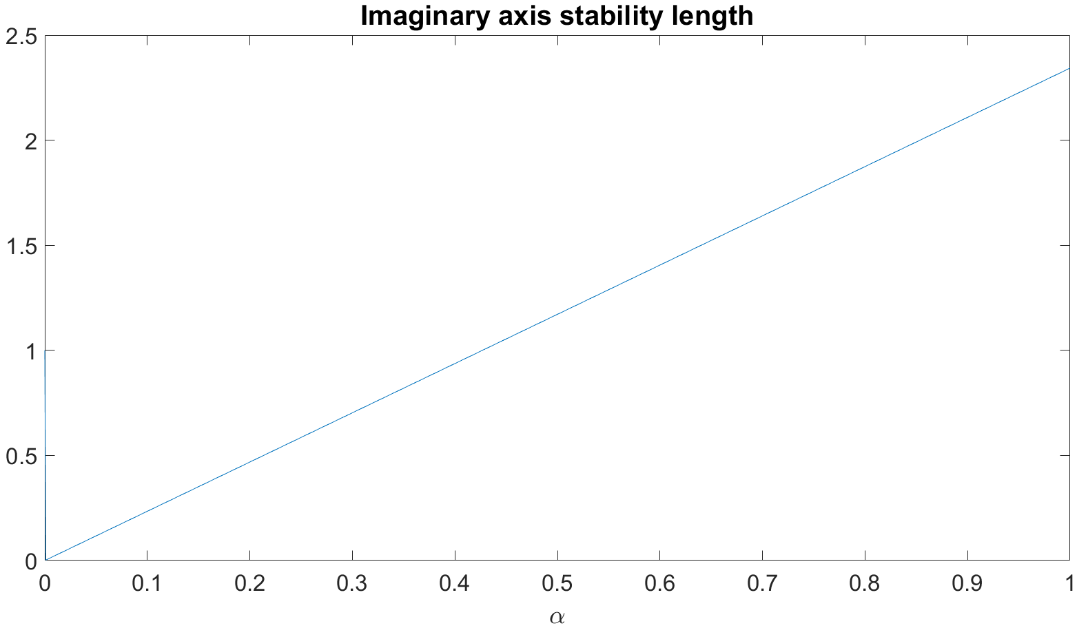
in the third stage of the explicit part of the method is arbitrary. In [23], the above value of α𝛼\alpha was chosen with the aim of maximizing the stability region of the method. However, if a stability and absolute monotonicity analysis is carried out, as discussed in detail in Appendix A, it can be seen that different choices might be more advantageous, in order to improve the monotonicity of the method without compromising its stability. In particular, the value of α=1/2𝛼12\alpha=1/2 appears to be a more appropriate choice, as also demonstrated by the numerical experiments reported in Section 7.

We now describe the application of this IMEX method and of the splitting approach outlined above to equations (2). Notice that, for simplicity, we first present the time semi-discretization only, while maintaining the continuous form of (2) with respect to the spatial variables. The detailed description of the algebraic problems resulting from the full space and time discretization according to the method outlined here will be presented in Section 5.

For each time step, we first consider the discretization of the hyperbolic and forcing terms. For the first stage of the method, one simply has

ρ(n,1)=ρn𝐮(n,1)=𝐮nE(n,1)=En.formulae-sequencesuperscript𝜌𝑛1superscript𝜌𝑛formulae-sequencesuperscript𝐮𝑛1superscript𝐮𝑛superscript𝐸𝑛1superscript𝐸𝑛\rho^{(n,1)}=\rho^{n}\ \ \ \ \mathbf{u}^{(n,1)}=\mathbf{u}^{n}\ \ \ \ E^{(n,1)}=E^{n}.

For the second stage, we can write formally

ρ(n,2)superscript𝜌𝑛2\displaystyle\rho^{(n,2)} =\displaystyle= ρna21Δt(ρn𝐮n)\displaystyle\rho^{n}-a_{21}\Delta t\operatorname{\nabla\cdot}\left(\rho^{n}\mathbf{u}^{n}\right)
ρ(n,2)𝐮(n,2)superscript𝜌𝑛2superscript𝐮𝑛2\displaystyle\rho^{(n,2)}\mathbf{u}^{(n,2)} +\displaystyle+ a~22ΔtM2p(n,2)=𝐦(n,2)subscript~𝑎22Δ𝑡superscript𝑀2superscript𝑝𝑛2superscript𝐦𝑛2\displaystyle\tilde{a}_{22}\frac{\Delta t}{M^{2}}\nabla p^{(n,2)}=\mathbf{m}^{(n,2)} (37)
ρ(n,2)E(n,2)superscript𝜌𝑛2superscript𝐸𝑛2\displaystyle\rho^{(n,2)}E^{(n,2)} +\displaystyle+ a~22Δt(h(n,2)ρ(n,2)𝐮(n,2))=e^(n,2),\displaystyle\tilde{a}_{22}\Delta t\operatorname{\nabla\cdot}\left(h^{(n,2)}\rho^{(n,2)}\mathbf{u}^{(n,2)}\right)=\hat{e}^{(n,2)},

where we have set

𝐦(n,2)superscript𝐦𝑛2\displaystyle\mathbf{m}^{(n,2)} =\displaystyle= ρn𝐮nsuperscript𝜌𝑛superscript𝐮𝑛\displaystyle\rho^{n}\mathbf{u}^{n} (38)
\displaystyle- a21Δt(ρn𝐮n𝐮n)a~21ΔtM2pna21ΔtFr2ρn𝐤\displaystyle a_{21}\Delta t\operatorname{\nabla\cdot}\left(\rho^{n}\mathbf{u}^{n}\otimes\mathbf{u}^{n}\right)-\tilde{a}_{21}\frac{\Delta t}{M^{2}}\nabla p^{n}-a_{21}\frac{\Delta t}{Fr^{2}}\rho^{n}\mathbf{k}
e^(n,2)superscript^𝑒𝑛2\displaystyle\hat{e}^{(n,2)} =\displaystyle= ρnEna~21Δt(hnρn𝐮n)a21ΔtM2(knρn𝐮n)\displaystyle\rho^{n}E^{n}-\tilde{a}_{21}\Delta t\operatorname{\nabla\cdot}\left(h^{n}\rho^{n}\mathbf{u}^{n}\right)-a_{21}\Delta tM^{2}\operatorname{\nabla\cdot}\left(k^{n}\rho^{n}\mathbf{u}^{n}\right)
\displaystyle- a21ΔtM2Fr2ρn𝐤𝐮n.subscript𝑎21Δ𝑡superscript𝑀2𝐹superscript𝑟2superscript𝜌𝑛𝐤superscript𝐮𝑛\displaystyle a_{21}\frac{\Delta tM^{2}}{Fr^{2}}\rho^{n}\mathbf{k}\cdot\mathbf{u}^{n}.

Notice that, substituting formally ρ(n,2)𝐮(n,2)superscript𝜌𝑛2superscript𝐮𝑛2\rho^{(n,2)}\mathbf{u}^{(n,2)} into the energy equation and taking into account the definitions ρE=ρe+ρk𝜌𝐸𝜌𝑒𝜌𝑘\rho E=\rho e+\rho k and h=e+p/ρ,𝑒𝑝𝜌h=e+p/\rho, the above system can be solved by computing the solution of

ρ(n,2)[e(p(n,2),ρ(n,2))+k(n,2)]superscript𝜌𝑛2delimited-[]𝑒superscript𝑝𝑛2superscript𝜌𝑛2superscript𝑘𝑛2\displaystyle\hskip 17.07182pt\rho^{(n,2)}[e(p^{(n,2)},\rho^{(n,2)})+k^{(n,2)}]
a~222Δt2M2[(e(p(n,2),ρ(n,2))+p(n,2)ρ(n,2))p(n,2)]\displaystyle-\hskip 5.69046pt\tilde{a}^{2}_{22}\frac{\Delta t^{2}}{M^{2}}\operatorname{\nabla\cdot}\left[\left(e(p^{(n,2)},\rho^{(n,2)})+\frac{p^{(n,2)}}{\rho^{(n,2)}}\right)\nabla p^{(n,2)}\right] (39)
+a~22Δt[(e(p(n,2),ρ(n,2))+p(n,2)ρ(n,2))𝐦(n,2)]=e^(n,2)\displaystyle+\hskip 5.69046pt\tilde{a}_{22}\Delta t\operatorname{\nabla\cdot}\left[\left(e(p^{(n,2)},\rho^{(n,2)})+\frac{p^{(n,2)}}{\rho^{(n,2)}}\right)\mathbf{m}^{(n,2)}\right]=\hat{e}^{(n,2)}

in terms of p(n,2)superscript𝑝𝑛2p^{(n,2)} according to the fixed point procedure described in [14]. More specifically, setting ξ(0)=p(n,2),k(n,2,0)=k(n,1),formulae-sequencesuperscript𝜉0superscript𝑝𝑛2superscript𝑘𝑛20superscript𝑘𝑛1\xi^{(0)}=p^{(n,2)},k^{(n,2,0)}=k^{(n,1)}, one solves for l=1,,L𝑙1𝐿l=1,\dots,L the equation

ρ(n,2)e(ξ(l+1),ρ(n,2))superscript𝜌𝑛2𝑒superscript𝜉𝑙1superscript𝜌𝑛2\displaystyle\rho^{(n,2)}e(\xi^{(l+1)},\rho^{(n,2)}) \displaystyle- a~222Δt2M2[(e(ξ(l),ρ(n,2))+ξ(l)ρ(n,2))ξ(l+1)]\displaystyle\tilde{a}^{2}_{22}\frac{\Delta t^{2}}{M^{2}}\operatorname{\nabla\cdot}\left[\left(e(\xi^{(l)},\rho^{(n,2)})+\frac{\xi^{(l)}}{\rho^{(n,2)}}\right)\nabla\xi^{(l+1)}\right]
=\displaystyle= e^(n,2)ρ(n,2)k(n,2,l)superscript^𝑒𝑛2superscript𝜌𝑛2superscript𝑘𝑛2𝑙\displaystyle\hat{e}^{(n,2)}-\rho^{(n,2)}k^{(n,2,l)}
\displaystyle- a~22Δt[(e(ξ(l),ρ(n,2))+ξ(l)ρ(n,2))𝐦(n,2)]\displaystyle\tilde{a}_{22}\Delta t\operatorname{\nabla\cdot}\left[\left(e(\xi^{(l)},\rho^{(n,2)})+\frac{\xi^{(l)}}{\rho^{(n,2)}}\right)\mathbf{m}^{(n,2)}\right]

and updates the velocity as

𝐮(n,2,l+1)+a~22Δtρ(n,2)M2ξ(l+1)=𝐦(n,2).superscript𝐮𝑛2𝑙1subscript~𝑎22Δ𝑡superscript𝜌𝑛2superscript𝑀2superscript𝜉𝑙1superscript𝐦𝑛2\mathbf{u}^{(n,2,l+1)}+\frac{\tilde{a}_{22}\Delta t}{\rho^{(n,2)}M^{2}}\nabla\xi^{(l+1)}=\mathbf{m}^{(n,2)}.

In the case of SG-EOS, ρ(n,2)e(ξ(l+1),ρ(n,2))superscript𝜌𝑛2𝑒superscript𝜉𝑙1superscript𝜌𝑛2\rho^{(n,2)}e\left(\xi^{(l+1)},\rho^{(n,2)}\right) contains a term that only depends on the density, as evident from Equation (17) and, therefore, it has to be properly considered in the right-hand side of (4). On the other hand, the general cubic EOS (10) contains products of quantities depending on temperature and on density. For the sake of simplicity, in order to avoid the solution of a nonlinear equation for each quadrature node, in these cases we keep the temperature at the value in the previous iteration of the fixed point procedure, so as to obtain:

c~v(T(ξ(l),ρ(n,2)))R~gξ(l+1)(1ρ(n,2)b~)subscript~𝑐𝑣𝑇superscript𝜉𝑙superscript𝜌𝑛2subscript~𝑅𝑔superscript𝜉𝑙11superscript𝜌𝑛2~𝑏\displaystyle\frac{\tilde{c}_{v}\left(T\left(\xi^{(l)},\rho^{(n,2)}\right)\right)}{\tilde{R}_{g}}\xi^{(l+1)}\left(1-\rho^{(n,2)}\tilde{b}\right) \displaystyle-
a~222Δt2M2[(e(ξ(l),ρ(n,2))+ξ(l)ρ(n,2))ξ(l+1)]\displaystyle\tilde{a}^{2}_{22}\frac{\Delta t^{2}}{M^{2}}\operatorname{\nabla\cdot}\left[\left(e\left(\xi^{(l)},\rho^{(n,2)}\right)+\frac{\xi^{(l)}}{\rho^{(n,2)}}\right)\nabla\xi^{(l+1)}\right] =\displaystyle=
e^(n,2)ρ(n,2)k(n,2,l)superscript^𝑒𝑛2superscript𝜌𝑛2superscript𝑘𝑛2𝑙\displaystyle\hat{e}^{(n,2)}-\rho^{(n,2)}k^{(n,2,l)} \displaystyle-
c~v(T(ξ(l),ρ(n,2)))R~ga~(T(ξ(l),ρ(n,2)))(ρ(n,2))2(1ρ(n,2)b~r1)(1ρ(n,2)b~r2)(1ρ(n,2)b~)subscript~𝑐𝑣𝑇superscript𝜉𝑙superscript𝜌𝑛2subscript~𝑅𝑔~𝑎𝑇superscript𝜉𝑙superscript𝜌𝑛2superscriptsuperscript𝜌𝑛221superscript𝜌𝑛2~𝑏subscript𝑟11superscript𝜌𝑛2~𝑏subscript𝑟21superscript𝜌𝑛2~𝑏\displaystyle\frac{\tilde{c}_{v}(T\left(\xi^{(l)},\rho^{(n,2)}\right))}{\tilde{R}_{g}}\frac{\tilde{a}\left(T\left(\xi^{(l)},\rho^{(n,2)}\right)\right)\left(\rho^{(n,2)}\right)^{2}}{\left(1-\rho^{(n,2)}\tilde{b}r_{1}\right)\left(1-\rho^{(n,2)}\tilde{b}r_{2}\right)}\left(1-\rho^{(n,2)}\tilde{b}\right) \displaystyle-
ρ(n,2)b~[a~(T(ξ(l),ρ(n,2)))T(ξ(l),ρ(n,2))da~dT(ξ(l),ρ(n,2))]U(ρ(n,2))superscript𝜌𝑛2~𝑏delimited-[]~𝑎𝑇superscript𝜉𝑙superscript𝜌𝑛2𝑇superscript𝜉𝑙superscript𝜌𝑛2𝑑~𝑎𝑑𝑇superscript𝜉𝑙superscript𝜌𝑛2𝑈superscript𝜌𝑛2\displaystyle\frac{\rho^{(n,2)}}{\tilde{b}}\left[\tilde{a}\left(T\left(\xi^{(l)},\rho^{(n,2)}\right)\right)-T\left(\xi^{(l)},\rho^{(n,2)}\right)\frac{d\tilde{a}}{dT}\left(\xi^{(l)},\rho^{(n,2)}\right)\right]U\left(\rho^{(n,2)}\right) \displaystyle-
a~22Δt[(e(ξ(l),ρ(n,2))+ξ(l)ρ(n,2))𝐦(n,2)].\displaystyle\tilde{a}_{22}\Delta t\operatorname{\nabla\cdot}\left[\left(e\left(\xi^{(l)},\rho^{(n,2)}\right)+\frac{\xi^{(l)}}{\rho^{(n,2)}}\right)\mathbf{m}^{(n,2)}\right]. (41)

The same considerations as in [14] apply concerning the favourable properties of the weakly nonlinear system resulting from the discrete form of (4). Once the iterations have been completed, one sets 𝐮(n,2)=𝐮(n,2,L+1)superscript𝐮𝑛2superscript𝐮𝑛2𝐿1\mathbf{u}^{(n,2)}=\mathbf{u}^{(n,2,L+1)} and E(n,2)superscript𝐸𝑛2E^{(n,2)} accordingly. For the third stage, one can write formally

ρ(n,3)superscript𝜌𝑛3\displaystyle\rho^{(n,3)} =\displaystyle= ρna31Δt(ρn𝐮n)a32Δt(ρ(n,2)𝐮(n,2))\displaystyle\rho^{n}-a_{31}\Delta t\operatorname{\nabla\cdot}\left(\rho^{n}\mathbf{u}^{n}\right)-a_{32}\Delta t\operatorname{\nabla\cdot}\left(\rho^{(n,2)}\mathbf{u}^{(n,2)}\right)
ρ(n,3)𝐮(n,3)superscript𝜌𝑛3superscript𝐮𝑛3\displaystyle\rho^{(n,3)}\mathbf{u}^{(n,3)} +\displaystyle+ a~33ΔtM2p(n,3)=𝐦(n,3)subscript~𝑎33Δ𝑡superscript𝑀2superscript𝑝𝑛3superscript𝐦𝑛3\displaystyle\tilde{a}_{33}\frac{\Delta t}{M^{2}}\nabla p^{(n,3)}=\mathbf{m}^{(n,3)} (42)
ρ(n,3)E(n,3)superscript𝜌𝑛3superscript𝐸𝑛3\displaystyle\rho^{(n,3)}E^{(n,3)} +\displaystyle+ a~33Δt(h(n,3)ρ(n,3)𝐮(n,3))=e^(n,3),\displaystyle\tilde{a}_{33}\Delta t\operatorname{\nabla\cdot}\left(h^{(n,3)}\rho^{(n,3)}\mathbf{u}^{(n,3)}\right)=\hat{e}^{(n,3)},

where the right hand sides are defined as

𝐦(n,3)superscript𝐦𝑛3\displaystyle\mathbf{m}^{(n,3)} =\displaystyle= ρn𝐮nsuperscript𝜌𝑛superscript𝐮𝑛\displaystyle\rho^{n}\mathbf{u}^{n}
\displaystyle- a31Δt(ρn𝐮n𝐮n)a~31ΔtM2pna31ΔtFr2ρn𝐤\displaystyle a_{31}\Delta t\operatorname{\nabla\cdot}\left(\rho^{n}\mathbf{u}^{n}\otimes\mathbf{u}^{n}\right)-\tilde{a}_{31}\frac{\Delta t}{M^{2}}\nabla p^{n}-a_{31}\frac{\Delta t}{Fr^{2}}\rho^{n}\mathbf{k}
\displaystyle- a32Δt(ρ(n,2)𝐮(n,2)𝐮(n,2))a~32ΔtM2p(n,2)a32ΔtFr2ρ(n,2)𝐤\displaystyle a_{32}\Delta t\operatorname{\nabla\cdot}\left(\rho^{(n,2)}\mathbf{u}^{(n,2)}\otimes\mathbf{u}^{(n,2)}\right)-\tilde{a}_{32}\frac{\Delta t}{M^{2}}\nabla p^{(n,2)}-a_{32}\frac{\Delta t}{Fr^{2}}\rho^{(n,2)}\mathbf{k}
e^(n,3)superscript^𝑒𝑛3\displaystyle\hat{e}^{(n,3)} =\displaystyle= ρnEna~31Δt(hnρn𝐮n)a31ΔtM2(knρn𝐮n)\displaystyle\rho^{n}E^{n}-\tilde{a}_{31}\Delta t\operatorname{\nabla\cdot}\left(h^{n}\rho^{n}\mathbf{u}^{n}\right)-a_{31}\Delta tM^{2}\operatorname{\nabla\cdot}\left(k^{n}\rho^{n}\mathbf{u}^{n}\right)
\displaystyle- a31ΔtM2Fr2ρn𝐤𝐮nsubscript𝑎31Δ𝑡superscript𝑀2𝐹superscript𝑟2superscript𝜌𝑛𝐤superscript𝐮𝑛\displaystyle a_{31}\Delta t\frac{M^{2}}{Fr^{2}}\rho^{n}\mathbf{k}\cdot\mathbf{u}^{n}
\displaystyle- a~32Δt(h(n,2)ρ(n,2)𝐮(n,2))a32ΔtM2(k(n,2)ρ(n,2)𝐮(n,2))\displaystyle\tilde{a}_{32}\Delta t\operatorname{\nabla\cdot}\left(h^{(n,2)}\rho^{(n,2)}\mathbf{u}^{(n,2)}\right)-a_{32}\Delta tM^{2}\operatorname{\nabla\cdot}\left(k^{(n,2)}\rho^{(n,2)}\mathbf{u}^{(n,2)}\right)
\displaystyle- a32ΔtM2Fr2ρ(n,2)𝐤𝐮(n,2).subscript𝑎32Δ𝑡superscript𝑀2𝐹superscript𝑟2superscript𝜌𝑛2𝐤superscript𝐮𝑛2\displaystyle a_{32}\Delta t\frac{M^{2}}{Fr^{2}}\rho^{(n,2)}\mathbf{k}\cdot\mathbf{u}^{(n,2)}.

Again, the solution of this stage is computed by substituting formally ρ(n,3)𝐮(n,3)superscript𝜌𝑛3superscript𝐮𝑛3\rho^{(n,3)}\mathbf{u}^{(n,3)} into the energy equation and computing the solution of

ρ(n,3)[e(p(n,3),ρ(n,3))+k(n,3)]superscript𝜌𝑛3delimited-[]𝑒superscript𝑝𝑛3superscript𝜌𝑛3superscript𝑘𝑛3\displaystyle\hskip 17.07182pt\rho^{(n,3)}[e\left(p^{(n,3)},\rho^{(n,3)}\right)+k^{(n,3)}] (44)
a~332Δt2M2[(e(p(n,3),ρ(n,3))+p(n,3)ρ(n,3))p(n,3)]\displaystyle-\hskip 5.69046pt\tilde{a}^{2}_{33}\frac{\Delta t^{2}}{M^{2}}\operatorname{\nabla\cdot}\left[\left(e\left(p^{(n,3)},\rho^{(n,3)}\right)+\frac{p^{(n,3)}}{\rho^{(n,3)}}\right)\nabla p^{(n,3)}\right]
+a~33Δt[(e(p(n,3),ρ(n,3))+p(n,3)ρ(n,3))𝐦(n,3)]=e^(n,3).\displaystyle+\hskip 5.69046pt\tilde{a}_{33}\Delta t\operatorname{\nabla\cdot}\left[\left(e\left(p^{(n,3)},\rho^{(n,3)}\right)+\frac{p^{(n,3)}}{\rho^{(n,3)}}\right)\mathbf{m}^{(n,3)}\right]=\hat{e}^{(n,3)}.

More specifically, setting ξ(0)=p(n,3),k(n,3,0)=k(n,2),formulae-sequencesuperscript𝜉0superscript𝑝𝑛3superscript𝑘𝑛30superscript𝑘𝑛2\xi^{(0)}=p^{(n,3)},k^{(n,3,0)}=k^{(n,2)}, one solves for l=1,,L𝑙1𝐿l=1,\dots,L the equation

ρ(n,3)e(ξ(l+1),ρ(n,3))superscript𝜌𝑛3𝑒superscript𝜉𝑙1superscript𝜌𝑛3\displaystyle\rho^{(n,3)}e\left(\xi^{(l+1)},\rho^{(n,3)}\right) \displaystyle- a~332Δt2M2[(e(ξ(l),ρ(n,3))+ξ(l)ρ(n,3))ξ(l+1)]\displaystyle\frac{\tilde{a}^{2}_{33}\Delta t^{2}}{M^{2}}\operatorname{\nabla\cdot}\left[\left(e(\xi^{(l)},\rho^{(n,3)})+\frac{\xi^{(l)}}{\rho^{(n,3)}}\right)\nabla\xi^{(l+1)}\right]
=\displaystyle= e^(n,3)ρ(n,3)k(n,3,l)superscript^𝑒𝑛3superscript𝜌𝑛3superscript𝑘𝑛3𝑙\displaystyle\hat{e}^{(n,3)}-\rho^{(n,3)}k^{(n,3,l)}
\displaystyle- a~33Δt[(e(ξ(l),ρ(n,3))+ξ(l)ρ(n,3))𝐦(n,3)]\displaystyle\tilde{a}_{33}\Delta t\operatorname{\nabla\cdot}\left[\left(e\left(\xi^{(l)},\rho^{(n,3)}\right)+\frac{\xi^{(l)}}{\rho^{(n,3)}}\right)\mathbf{m}^{(n,3)}\right]

and updates the velocity as

𝐮(n,3,l+1)+a~33Δtρ(n,3)M2ξ(l+1)=𝐦(n,3).superscript𝐮𝑛3𝑙1subscript~𝑎33Δ𝑡superscript𝜌𝑛3superscript𝑀2superscript𝜉𝑙1superscript𝐦𝑛3\mathbf{u}^{(n,3,l+1)}+\tilde{a}_{33}\frac{\Delta t}{\rho^{(n,3)}M^{2}}\nabla\xi^{(l+1)}=\mathbf{m}^{(n,3)}.

Once again, in case of a non-ideal gas equation of state, the expression of ρ(n,3)e(ξ(l+1),ρ(n,3))superscript𝜌𝑛3𝑒superscript𝜉𝑙1superscript𝜌𝑛3\rho^{(n,3)}e\left(\xi^{(l+1)},\rho^{(n,3)}\right) is slightly different. For the sake of clarity, we report also for this stage the fixed point equation for the general cubic EOS:

c~v(T(ξ(l),ρ(n,3)))R~gξ(l+1)(1ρ(n,3)b~)subscript~𝑐𝑣𝑇superscript𝜉𝑙superscript𝜌𝑛3subscript~𝑅𝑔superscript𝜉𝑙11superscript𝜌𝑛3~𝑏\displaystyle\frac{\tilde{c}_{v}\left(T\left(\xi^{(l)},\rho^{(n,3)}\right)\right)}{\tilde{R}_{g}}\xi^{(l+1)}\left(1-\rho^{(n,3)}\tilde{b}\right) \displaystyle-
a~332Δt2M2[(e(ξ(l),ρ(n,3))+ξ(l)ρ(n,3))ξ(l+1)]\displaystyle\tilde{a}^{2}_{33}\frac{\Delta t^{2}}{M^{2}}\operatorname{\nabla\cdot}\left[\left(e\left(\xi^{(l)},\rho^{(n,3)}\right)+\frac{\xi^{(l)}}{\rho^{(n,3)}}\right)\nabla\xi^{(l+1)}\right] =\displaystyle=
e^(n,3)ρ(n,3)k(n,3,l)superscript^𝑒𝑛3superscript𝜌𝑛3superscript𝑘𝑛3𝑙\displaystyle\hat{e}^{(n,3)}-\rho^{(n,3)}k^{(n,3,l)} \displaystyle-
c~v(T(ξ(l),ρ(n,3)))R~ga~(T(ξ(l),ρ(n,3)))(ρ(n,3))2(1ρ(n,3)b~r1)(1ρ(n,3)b~r2)(1ρ(n,3)b~)subscript~𝑐𝑣𝑇superscript𝜉𝑙superscript𝜌𝑛3subscript~𝑅𝑔~𝑎𝑇superscript𝜉𝑙superscript𝜌𝑛3superscriptsuperscript𝜌𝑛321superscript𝜌𝑛3~𝑏subscript𝑟11superscript𝜌𝑛3~𝑏subscript𝑟21superscript𝜌𝑛3~𝑏\displaystyle\frac{\tilde{c}_{v}\left(T\left(\xi^{(l)},\rho^{(n,3)}\right)\right)}{\tilde{R}_{g}}\frac{\tilde{a}\left(T\left(\xi^{(l)},\rho^{(n,3)}\right)\right)\left(\rho^{(n,3)}\right)^{2}}{\left(1-\rho^{(n,3)}\tilde{b}r_{1}\right)\left(1-\rho^{(n,3)}\tilde{b}r_{2}\right)}\left(1-\rho^{(n,3)}\tilde{b}\right) \displaystyle-
ρ(n,3)b~[a~(T(ξ(l),ρ(n,3)))T(ξ(l),ρ(n,3))da~dT(ξ(l),ρ(n,3))]U(ρ(n,3))superscript𝜌𝑛3~𝑏delimited-[]~𝑎𝑇superscript𝜉𝑙superscript𝜌𝑛3𝑇superscript𝜉𝑙superscript𝜌𝑛3𝑑~𝑎𝑑𝑇superscript𝜉𝑙superscript𝜌𝑛3𝑈superscript𝜌𝑛3\displaystyle\frac{\rho^{(n,3)}}{\tilde{b}}\left[\tilde{a}\left(T\left(\xi^{(l)},\rho^{(n,3)}\right)\right)-T\left(\xi^{(l)},\rho^{(n,3)}\right)\frac{d\tilde{a}}{dT}\left(\xi^{(l)},\rho^{(n,3)}\right)\right]U\left(\rho^{(n,3)}\right) \displaystyle-
a~33Δt[(e(ξ(l),ρ(n,3))+ξ(l)ρ(n,3))𝐦(n,3)].\displaystyle\tilde{a}_{33}\Delta t\operatorname{\nabla\cdot}\left[\left(e\left(\xi^{(l)},\rho^{(n,3)}\right)+\frac{\xi^{(l)}}{\rho^{(n,3)}}\right)\mathbf{m}^{(n,3)}\right]. (46)

Let us consider now the diffusive part of the Navier-Stokes equations that, as already mentioned in Section 1, will be treated with an operator splitting technique. For the sake of clarity, we denote with similar-to\sim the quantities computed in this part of the scheme; hence, we define

𝐮~(n,1)=𝐮(n,3)E~(n,1)=E(n,3)formulae-sequencesuperscript~𝐮𝑛1superscript𝐮𝑛3superscript~𝐸𝑛1superscript𝐸𝑛3\mathbf{\tilde{u}}^{(n,1)}=\mathbf{u}^{(n,3)}\qquad{\tilde{E}}^{(n,1)}=E^{(n,3)}

and we proceed to the discretization of the viscous terms, which is carried out by the implicit part of the IMEX method previously described:

ρn+1𝐮~(n,2)superscript𝜌𝑛1superscript~𝐮𝑛2\displaystyle\rho^{n+1}\mathbf{\tilde{u}}^{(n,2)} \displaystyle- a~22ΔtRe[(𝐮~+𝐮~T)23(𝐮~)𝐈](n,2)=𝐦~(n,2)\displaystyle\tilde{a}_{22}\frac{\Delta t}{Re}\operatorname{\nabla\cdot}\left[\left(\nabla\mathbf{\tilde{u}}+\nabla\mathbf{\tilde{u}}^{T}\right)-\frac{2}{3}(\nabla\cdot\mathbf{\tilde{u}})\mathbf{I}\right]^{(n,2)}=\mathbf{\tilde{m}}^{(n,2)} (47)
ρn+1E~(n,2)superscript𝜌𝑛1superscript~𝐸𝑛2\displaystyle\rho^{n+1}\tilde{E}^{(n,2)} \displaystyle- a~22ΔtM2Re[(𝐮~+𝐮~T)𝐮~23(𝐮~)𝐮~](n,2)\displaystyle\tilde{a}_{22}\frac{\Delta tM^{2}}{Re}\operatorname{\nabla\cdot}\left[\left(\nabla\mathbf{\tilde{u}}+\nabla\mathbf{\tilde{u}}^{T}\right)\mathbf{\tilde{u}}-\frac{2}{3}(\nabla\cdot\mathbf{\tilde{u}})\mathbf{\tilde{u}}\right]^{(n,2)}
\displaystyle- a~22ΔtPrReΔT~(n,2)=e~(n,2),subscript~𝑎22Δ𝑡𝑃𝑟𝑅𝑒Δsuperscript~𝑇𝑛2superscript~𝑒𝑛2\displaystyle\tilde{a}_{22}\frac{\Delta t}{PrRe}\Delta\tilde{T}^{(n,2)}={\tilde{e}}^{(n,2)},

where we have set

𝐦~(n,2)superscript~𝐦𝑛2\displaystyle\mathbf{\tilde{m}}^{(n,2)} =\displaystyle= ρn+1𝐮~(n,1)+a~21ΔtRe[(𝐮~+𝐮~T)23(𝐮~)𝐈](n,1)\displaystyle\rho^{n+1}\mathbf{\tilde{u}}^{(n,1)}+\tilde{a}_{21}\frac{\Delta t}{Re}\operatorname{\nabla\cdot}\left[\left(\nabla\mathbf{\tilde{u}}+\nabla\mathbf{\tilde{u}}^{T}\right)-\frac{2}{3}(\nabla\cdot\mathbf{\tilde{u}})\mathbf{I}\right]^{(n,1)}
e~(n,2)superscript~𝑒𝑛2\displaystyle{\tilde{e}}^{(n,2)} =\displaystyle= ρn+1E~(n,1)superscript𝜌𝑛1superscript~𝐸𝑛1\displaystyle\rho^{n+1}\tilde{E}^{(n,1)}
+\displaystyle+ a~21ΔtM2Re[(𝐮+𝐮T)𝐮23(𝐮)𝐮](n,1)\displaystyle\tilde{a}_{21}\frac{\Delta tM^{2}}{Re}\operatorname{\nabla\cdot}\left[\left(\nabla\mathbf{u}+\nabla\mathbf{u}^{T}\right)\mathbf{u}-\frac{2}{3}(\nabla\cdot\mathbf{u})\mathbf{u}\right]^{(n,1)}
+\displaystyle+ a~21ΔtPrReΔT~(n,1).subscript~𝑎21Δ𝑡𝑃𝑟𝑅𝑒Δsuperscript~𝑇𝑛1\displaystyle\tilde{a}_{21}\frac{\Delta t}{PrRe}\Delta\tilde{T}^{(n,1)}.

Notice that the momentum equation in (47) is decoupled from the energy equation and can be solved independently, so that in a subsequent step the equation for E~(n,2)superscript~𝐸𝑛2\tilde{E}^{(n,2)} can be solved using temperature as an unknown. It is worth to mention that, in case dadT0𝑑𝑎𝑑𝑇0\frac{da}{dT}\neq 0 or dcvdT0𝑑subscript𝑐𝑣𝑑𝑇0\frac{dc_{v}}{dT}\neq 0, for the cubic EOS, we end up with a non-linear equation. The following fixed point procedure is considered: setting ξ(0)=T~(n,1),superscript𝜉0superscript~𝑇𝑛1\xi^{(0)}=\tilde{T}^{(n,1)}, one solves for l=1,,L𝑙1𝐿l=1,\dots,L

c~v(ξ(l))ξ(l+1)+a~(ξ(l))ξ(l+1)da~dT(ξ(l))bsubscript~𝑐𝑣superscript𝜉𝑙superscript𝜉𝑙1~𝑎superscript𝜉𝑙superscript𝜉𝑙1𝑑~𝑎𝑑𝑇superscript𝜉𝑙𝑏\displaystyle\tilde{c}_{v}\left(\xi^{(l)}\right)\xi^{(l+1)}+\frac{\tilde{a}\left(\xi^{(l)}\right)-\xi^{(l+1)}\frac{d\tilde{a}}{dT}\left(\xi^{(l)}\right)}{b}
a~22ΔtM2Re[(𝐮~+𝐮~T)𝐮~23(𝐮~)𝐮~](n,2)\displaystyle-\tilde{a}_{22}\frac{\Delta tM^{2}}{Re}\operatorname{\nabla\cdot}\left[\left(\nabla\mathbf{\tilde{u}}+\nabla\mathbf{\tilde{u}}^{T}\right)\mathbf{\tilde{u}}-\frac{2}{3}(\nabla\cdot\mathbf{\tilde{u}})\mathbf{\tilde{u}}\right]^{(n,2)}
a~22ΔtPrReΔξ(l+1)=e~(n,2).subscript~𝑎22Δ𝑡𝑃𝑟𝑅𝑒Δsuperscript𝜉𝑙1superscript~𝑒𝑛2\displaystyle-\tilde{a}_{22}\frac{\Delta t}{PrRe}\Delta\xi^{(l+1)}={\tilde{e}}^{(n,2)}. (48)

For the third stage, one can write formally

ρn+1𝐮~(n,3)superscript𝜌𝑛1superscript~𝐮𝑛3\displaystyle\rho^{n+1}\mathbf{\tilde{u}}^{(n,3)} \displaystyle- a~33ΔtRe[(𝐮~+𝐮~T)23(𝐮~)𝐈](n,3)=𝐦~(n,3)\displaystyle\tilde{a}_{33}\frac{\Delta t}{Re}\operatorname{\nabla\cdot}\left[\left(\nabla\mathbf{\tilde{u}}+\nabla\mathbf{\tilde{u}}^{T}\right)-\frac{2}{3}(\nabla\cdot\mathbf{\tilde{u}})\mathbf{I}\right]^{(n,3)}=\mathbf{\tilde{m}}^{(n,3)}
ρn+1E~(n,3)superscript𝜌𝑛1superscript~𝐸𝑛3\displaystyle\rho^{n+1}\tilde{E}^{(n,3)} \displaystyle- a~33ΔtM2Re[(𝐮~+𝐮~T)𝐮~23(𝐮~)𝐮~](n,3)\displaystyle\tilde{a}_{33}\frac{\Delta tM^{2}}{Re}\operatorname{\nabla\cdot}\left[\left(\nabla\mathbf{\tilde{u}}+\nabla\mathbf{\tilde{u}}^{T}\right)\mathbf{\tilde{u}}-\frac{2}{3}(\nabla\cdot\mathbf{\tilde{u}})\mathbf{\tilde{u}}\right]^{(n,3)}
\displaystyle- a~33ΔtPrReΔT~(n,3)=𝐞~(n,3),subscript~𝑎33Δ𝑡𝑃𝑟𝑅𝑒Δsuperscript~𝑇𝑛3superscript~𝐞𝑛3\displaystyle\tilde{a}_{33}\frac{\Delta t}{PrRe}\Delta\tilde{T}^{(n,3)}=\mathbf{\tilde{e}}^{(n,3)},

where the right hand sides are defined as

𝐦~(n,3)superscript~𝐦𝑛3\displaystyle\mathbf{\tilde{m}}^{(n,3)} =\displaystyle= ρn+1𝐮~(n,1)+a~31ΔtRe[(𝐮~+𝐮~T)23(𝐮~)𝐈](n,1)\displaystyle\rho^{n+1}\mathbf{\tilde{u}}^{(n,1)}+\tilde{a}_{31}\frac{\Delta t}{Re}\operatorname{\nabla\cdot}\left[\left(\nabla\mathbf{\tilde{u}}+\nabla\mathbf{\tilde{u}}^{T}\right)-\frac{2}{3}(\nabla\cdot\mathbf{\tilde{u}})\mathbf{I}\right]^{(n,1)} (49)
+\displaystyle+ a~32ΔtRe[(𝐮~+𝐮~T)23(𝐮~)𝐈](n,2)\displaystyle\tilde{a}_{32}\frac{\Delta t}{Re}\operatorname{\nabla\cdot}\left[\left(\nabla\mathbf{\tilde{u}}+\nabla\mathbf{\tilde{u}}^{T}\right)-\frac{2}{3}(\nabla\cdot\mathbf{\tilde{u}})\mathbf{I}\right]^{(n,2)}
𝐞~(n,3)superscript~𝐞𝑛3\displaystyle\mathbf{\tilde{e}}^{(n,3)} =\displaystyle= ρn+1E~(n,1)superscript𝜌𝑛1superscript~𝐸𝑛1\displaystyle\rho^{n+1}\tilde{E}^{(n,1)}
+\displaystyle+ a~31ΔtM2Re[(𝐮~+𝐮~T)𝐮~23(𝐮~)𝐮~](n,1)\displaystyle\tilde{a}_{31}\frac{\Delta tM^{2}}{Re}\operatorname{\nabla\cdot}\left[\left(\nabla\mathbf{\tilde{u}}+\nabla\mathbf{\tilde{u}}^{T}\right)\mathbf{\tilde{u}}-\frac{2}{3}(\nabla\cdot\mathbf{\tilde{u}})\mathbf{\tilde{u}}\right]^{(n,1)}
+\displaystyle+ a~32ΔtM2Re[(𝐮~+𝐮~T)𝐮~23(𝐮~)𝐮~](n,2)\displaystyle\tilde{a}_{32}\frac{\Delta tM^{2}}{Re}\operatorname{\nabla\cdot}\left[\left(\nabla\mathbf{\tilde{u}}+\nabla\mathbf{\tilde{u}}^{T}\right)\mathbf{\tilde{u}}-\frac{2}{3}(\nabla\cdot\mathbf{\tilde{u}})\mathbf{\tilde{u}}\right]^{(n,2)}
+\displaystyle+ a~31ΔtPrReΔT~(n,1)+a~32ΔtPrReΔT~(n,2).subscript~𝑎31Δ𝑡𝑃𝑟𝑅𝑒Δsuperscript~𝑇𝑛1subscript~𝑎32Δ𝑡𝑃𝑟𝑅𝑒Δsuperscript~𝑇𝑛2\displaystyle\tilde{a}_{31}\frac{\Delta t}{PrRe}\Delta\tilde{T}^{(n,1)}+\tilde{a}_{32}\frac{\Delta t}{PrRe}\Delta\tilde{T}^{(n,2)}.

Again, the momentum equation in (4) is decoupled from the energy equation and can be solved independently, so that in a subsequent step the equation for E(n,3)superscript𝐸𝑛3E^{(n,3)} can be solved using temperature as an unkown. Finally, one sets

𝐮n+1=𝐮~(n,3)En+1=E~(n,3)formulae-sequencesuperscript𝐮𝑛1superscript~𝐮𝑛3superscript𝐸𝑛1superscript~𝐸𝑛3\mathbf{u}^{n+1}=\mathbf{\tilde{u}}^{(n,3)}\ \ \ \ E^{n+1}=\tilde{E}^{(n,3)}

and the computation of the nlimit-from𝑛n-th time step is completed.

5 The spatial discretization strategy

We consider a decomposition of the domain ΩΩ\Omega into a family of hexahedra 𝒯hsubscript𝒯\mathcal{T}_{h} (quadrilaterals in the two-dimensional case) and denote each element by K𝐾K. The skeleton \mathcal{E} denotes the set of all element faces and =IBsuperscript𝐼superscript𝐵\mathcal{E}=\mathcal{E}^{I}\cup\mathcal{E}^{B}, where Isuperscript𝐼\mathcal{E}^{I} is the subset of interior faces and Bsuperscript𝐵\mathcal{E}^{B} is the subset of boundary faces. Suitable jump and average operators can then be defined as customary for finite element discretizations. A face ΓIΓsuperscript𝐼\Gamma\in\mathcal{E}^{I} shares two elements that we denote by K+superscript𝐾K^{+} with outward unit normal 𝐧+superscript𝐧\mathbf{n}^{+} and Ksuperscript𝐾K^{-} with outward unit normal 𝐧superscript𝐧\mathbf{n}^{-}, whereas for a face ΓBΓsuperscript𝐵\Gamma\in\mathcal{E}^{B} we denote by 𝐧𝐧\mathbf{n} the outward unit normal. For a scalar function φ𝜑\varphi the jump is defined as

[[φ]]=φ+𝐧++φ𝐧if ΓI[[φ]]=φ𝐧if ΓB.formulae-sequencedelimited-[]delimited-[]𝜑superscript𝜑superscript𝐧superscript𝜑superscript𝐧formulae-sequenceif Γsuperscript𝐼formulae-sequencedelimited-[]delimited-[]𝜑𝜑𝐧if Γsuperscript𝐵\left[\left[\varphi\right]\right]=\varphi^{+}\mathbf{n}^{+}+\varphi^{-}\mathbf{n}^{-}\quad\text{if }\Gamma\in\mathcal{E}^{I}\qquad\left[\left[\varphi\right]\right]=\varphi\mathbf{n}\quad\text{if }\Gamma\in\mathcal{E}^{B}.

The average is defined as

{{φ}}=12(φ++φ)if ΓI{{φ}}=φif ΓB.formulae-sequence𝜑12superscript𝜑superscript𝜑formulae-sequenceif Γsuperscript𝐼formulae-sequence𝜑𝜑if Γsuperscript𝐵\left\{\left\{\varphi\right\}\right\}=\frac{1}{2}\left(\varphi^{+}+\varphi^{-}\right)\quad\text{if }\Gamma\in\mathcal{E}^{I}\qquad\left\{\left\{\varphi\right\}\right\}=\varphi\quad\text{if }\Gamma\in\mathcal{E}^{B}.

Similar definitions apply for a vector function 𝝋𝝋\boldsymbol{\varphi}:

[[𝝋]]=𝝋+𝐧++𝝋𝐧if ΓI[[𝝋]]=𝝋𝐧if ΓBformulae-sequencedelimited-[]delimited-[]𝝋superscript𝝋superscript𝐧superscript𝝋superscript𝐧formulae-sequenceif Γsuperscript𝐼formulae-sequencedelimited-[]delimited-[]𝝋𝝋𝐧if Γsuperscript𝐵\displaystyle\left[\left[\boldsymbol{\varphi}\right]\right]=\boldsymbol{\varphi}^{+}\cdot\mathbf{n}^{+}+\boldsymbol{\varphi}^{-}\cdot\mathbf{n}^{-}\quad\text{if }\Gamma\in\mathcal{E}^{I}\qquad\left[\left[\boldsymbol{\varphi}\right]\right]=\boldsymbol{\varphi}\cdot\mathbf{n}\quad\text{if }\Gamma\in\mathcal{E}^{B}
{{𝝋}}=12(𝝋++𝝋)if ΓI{{𝝋}}=𝝋if ΓB.formulae-sequence𝝋12superscript𝝋superscript𝝋formulae-sequenceif Γsuperscript𝐼formulae-sequence𝝋𝝋if Γsuperscript𝐵\displaystyle\left\{\left\{\boldsymbol{\varphi}\right\}\right\}=\frac{1}{2}\left(\boldsymbol{\varphi}^{+}+\boldsymbol{\varphi}^{-}\right)\quad\text{if }\Gamma\in\mathcal{E}^{I}\qquad\left\{\left\{\boldsymbol{\varphi}\right\}\right\}=\boldsymbol{\varphi}\quad\text{if }\Gamma\in\mathcal{E}^{B}.

For vector functions, it is also useful to define a tensor jump as:

𝝋=𝝋+𝐧++𝝋𝐧if ΓI𝝋=𝝋𝐧if ΓB.formulae-sequencedelimited-⟨⟩delimited-⟨⟩𝝋tensor-productsuperscript𝝋superscript𝐧tensor-productsuperscript𝝋superscript𝐧formulae-sequenceif Γsuperscript𝐼formulae-sequencedelimited-⟨⟩delimited-⟨⟩𝝋tensor-product𝝋𝐧if Γsuperscript𝐵\left<\left<\boldsymbol{\varphi}\right>\right>=\boldsymbol{\varphi}^{+}\otimes\mathbf{n}^{+}+\boldsymbol{\varphi}^{-}\otimes\mathbf{n}^{-}\quad\text{if }\Gamma\in\mathcal{E}^{I}\qquad\left<\left<\boldsymbol{\varphi}\right>\right>=\boldsymbol{\varphi}\otimes\mathbf{n}\quad\text{if }\Gamma\in\mathcal{E}^{B}.

We also introduce the following finite element spaces

Qr={vL2(Ω):v|KrK𝒯h}𝐕r=[Qr]d,Q_{r}=\left\{v\in L^{2}(\Omega):v\rvert_{K}\in\mathbb{Q}_{r}\quad\forall K\in\mathcal{T}_{h}\right\}\ \ \ \mathbf{V}_{r}=\left[Q_{r}\right]^{d},

where rsubscript𝑟\mathbb{Q}_{r} is the space of polynomials of degree r𝑟r in each coordinate direction. We then denote by 𝝋i(𝐱)subscript𝝋𝑖𝐱\boldsymbol{\varphi}_{i}(\mathbf{x}) the basis functions for the space 𝐕rsubscript𝐕𝑟\mathbf{V}_{r} and by ψi(𝐱)subscript𝜓𝑖𝐱\psi_{i}(\mathbf{x}) the basis functions for the space Qrsubscript𝑄𝑟Q_{r}, the finite element spaces chosen for the discretization of the velocity and of the pressure (as well as the density), respectively.

𝐮j=1dim(𝐕r)uj(t)𝝋j(𝐱)pj=1dim(Qr)pj(t)ψj(𝐱).formulae-sequence𝐮superscriptsubscript𝑗1dimsubscript𝐕𝑟subscript𝑢𝑗𝑡subscript𝝋𝑗𝐱𝑝superscriptsubscript𝑗1dimsubscript𝑄𝑟subscript𝑝𝑗𝑡subscript𝜓𝑗𝐱\mathbf{u}\approx\sum_{j=1}^{\text{dim}(\mathbf{V}_{r})}u_{j}(t)\boldsymbol{\varphi}_{j}(\mathbf{x})\qquad p\approx\sum_{j=1}^{\text{dim}(Q_{r})}p_{j}(t)\psi_{j}(\mathbf{x}).

Given these definitions, the weak formulation for the momentum equation of the second stage (4) reads as follows:

KKρ(n,2)𝐮(n,2)𝐯𝑑Ωsubscript𝐾subscript𝐾superscript𝜌𝑛2superscript𝐮𝑛2𝐯differential-dΩ\displaystyle\qquad\sum_{K}\int_{K}\rho^{(n,2)}\mathbf{u}^{(n,2)}\cdot\mathbf{v}d\Omega
KKa~22ΔtM2p(n,2)𝐯𝑑Ω+ΓΓa~22ΔtM2{{p(n,2)}}[[𝐯]]𝑑Σsubscript𝐾subscript𝐾subscript~𝑎22Δ𝑡superscript𝑀2superscript𝑝𝑛2𝐯differential-dΩsubscriptΓsubscriptΓsubscript~𝑎22Δ𝑡superscript𝑀2superscript𝑝𝑛2delimited-[]delimited-[]𝐯differential-dΣ\displaystyle-\quad\sum_{K}\int_{K}\tilde{a}_{22}\frac{\Delta t}{M^{2}}p^{(n,2)}\nabla\cdot\mathbf{v}d\Omega+\sum_{\Gamma\in\mathcal{E}}\int_{\Gamma}\tilde{a}_{22}\frac{\Delta t}{M^{2}}\left\{\left\{p^{(n,2)}\right\}\right\}\left[\left[\mathbf{v}\right]\right]d\Sigma
=KKρn𝐮n𝐯𝑑ΩKKa21ΔtFr2ρn𝐤𝐯𝑑Ωsubscript𝐾subscript𝐾superscript𝜌𝑛superscript𝐮𝑛𝐯differential-dΩsubscript𝐾subscript𝐾subscript𝑎21Δ𝑡𝐹superscript𝑟2superscript𝜌𝑛𝐤𝐯differential-dΩ\displaystyle=\quad\sum_{K}\int_{K}\rho^{n}\mathbf{u}^{n}\cdot\mathbf{v}d\Omega-\sum_{K}\int_{K}a_{21}\frac{\Delta t}{Fr^{2}}\rho^{n}\mathbf{k}\cdot\mathbf{v}d\Omega
+KKa21Δt(ρn𝐮n𝐮n):𝐯dΩ+KKa~21ΔtM2pn𝐯𝑑Ω:subscript𝐾subscript𝐾subscript𝑎21Δ𝑡tensor-productsuperscript𝜌𝑛superscript𝐮𝑛superscript𝐮𝑛𝐯𝑑Ωsubscript𝐾subscript𝐾subscript~𝑎21Δ𝑡superscript𝑀2superscript𝑝𝑛𝐯differential-dΩ\displaystyle+\quad\sum_{K}\int_{K}a_{21}\Delta t\left(\rho^{n}\mathbf{u}^{n}\otimes\mathbf{u}^{n}\right):\nabla\mathbf{v}d\Omega+\sum_{K}\int_{K}\tilde{a}_{21}\frac{\Delta t}{M^{2}}p^{n}\nabla\cdot\mathbf{v}d\Omega
ΓΓa21Δt{{ρn𝐮n𝐮n}}:𝐯dΣ:subscriptΓsubscriptΓsubscript𝑎21Δ𝑡tensor-productsuperscript𝜌𝑛superscript𝐮𝑛superscript𝐮𝑛delimited-⟨⟩delimited-⟨⟩𝐯𝑑Σ\displaystyle-\quad\sum_{\Gamma\in\mathcal{E}}\int_{\Gamma}a_{21}\Delta t\left\{\left\{\rho^{n}\mathbf{u}^{n}\otimes\mathbf{u}^{n}\right\}\right\}:\left<\left<\mathbf{v}\right>\right>d\Sigma
ΓΓa~21ΔtM2{{pn}}[[𝐯]]𝑑ΣsubscriptΓsubscriptΓsubscript~𝑎21Δ𝑡superscript𝑀2superscript𝑝𝑛delimited-[]delimited-[]𝐯differential-dΣ\displaystyle-\quad\sum_{\Gamma\in\mathcal{E}}\int_{\Gamma}\tilde{a}_{21}\frac{\Delta t}{M^{2}}\left\{\left\{p^{n}\right\}\right\}\left[\left[\mathbf{v}\right]\right]d\Sigma
ΓΓa21Δtλ(n,1)2ρn𝐮n:𝐯dΣ,:subscriptΓsubscriptΓsubscript𝑎21Δ𝑡superscript𝜆𝑛12delimited-⟨⟩delimited-⟨⟩superscript𝜌𝑛superscript𝐮𝑛delimited-⟨⟩delimited-⟨⟩𝐯𝑑Σ\displaystyle-\quad\sum_{\Gamma\in\mathcal{E}}\int_{\Gamma}a_{21}\Delta t\frac{\lambda^{(n,1)}}{2}\left<\left<\rho^{n}\mathbf{u}^{n}\right>\right>:\left<\left<\mathbf{v}\right>\right>d\Sigma, (51)

where

λ(n,1)=max(|𝐮n+𝐧+|,|𝐮n𝐧|).superscript𝜆𝑛1superscript𝐮superscript𝑛superscript𝐧superscript𝐮superscript𝑛superscript𝐧\lambda^{(n,1)}=\max\left(\left|\mathbf{u}^{n^{+}}\cdot\mathbf{n}^{+}\right|,\left|\mathbf{u}^{n^{-}}\cdot\mathbf{n}^{-}\right|\right).

One can notice that centered flux has been employed as numerical flux for the quantities defined implicitly, whereas an upwind flux has been used for the quantities computed explicitly. In view of the implicit coupling between the momentum and the energy equations, we need to derive the algebraic formulation of (5) in order to formally substitute the degrees of freedom of the velocity into the algebraic formulation of the energy equation. We take 𝐯=𝝋i𝐯subscript𝝋𝑖\mathbf{v}=\boldsymbol{\varphi}_{i}, i=1dim(𝐕r)𝑖1dimsubscript𝐕𝑟i=1...\text{dim}(\mathbf{V}_{r}) and we exploit the representation introduced above to obtain

KKρ(n,2)j=1dim(𝐕r)uj(n,2)𝝋j𝝋idΩKKa~22ΔtM2j=1dim(Qr)pj(n,2)ψj𝝋idΩsubscript𝐾subscript𝐾superscript𝜌𝑛2superscriptsubscript𝑗1dimsubscript𝐕𝑟superscriptsubscript𝑢𝑗𝑛2subscript𝝋𝑗subscript𝝋𝑖𝑑Ωsubscript𝐾subscript𝐾subscript~𝑎22Δ𝑡superscript𝑀2superscriptsubscript𝑗1dimsubscript𝑄𝑟superscriptsubscript𝑝𝑗𝑛2subscript𝜓𝑗subscript𝝋𝑖𝑑Ω\displaystyle\qquad\sum_{K}\int_{K}\rho^{(n,2)}\sum_{j=1}^{\text{dim}(\mathbf{V}_{r})}u_{j}^{(n,2)}\boldsymbol{\varphi}_{j}\cdot\boldsymbol{\varphi}_{i}d\Omega-\sum_{K}\int_{K}\tilde{a}_{22}\frac{\Delta t}{M^{2}}\sum_{j=1}^{\text{dim}(Q_{r})}p_{j}^{(n,2)}\psi_{j}\nabla\cdot\boldsymbol{\varphi}_{i}d\Omega
+ΓΓa~22ΔtM2j=1dim(Qr)pj(n,2){{ψj}}[[𝝋i]]dΣsubscriptΓsubscriptΓsubscript~𝑎22Δ𝑡superscript𝑀2superscriptsubscript𝑗1dimsubscript𝑄𝑟superscriptsubscript𝑝𝑗𝑛2subscript𝜓𝑗delimited-[]delimited-[]subscript𝝋𝑖𝑑Σ\displaystyle+\quad\sum_{\Gamma\in\mathcal{E}}\int_{\Gamma}\tilde{a}_{22}\frac{\Delta t}{M^{2}}\sum_{j=1}^{\text{dim}(Q_{r})}p_{j}^{(n,2)}\left\{\left\{\psi_{j}\right\}\right\}\left[\left[\boldsymbol{\varphi}_{i}\right]\right]d\Sigma
=KKρn𝐮n𝝋i𝑑ΩKKa21ΔtFr2ρn𝐤𝝋i𝑑Ωsubscript𝐾subscript𝐾superscript𝜌𝑛superscript𝐮𝑛subscript𝝋𝑖differential-dΩsubscript𝐾subscript𝐾subscript𝑎21Δ𝑡𝐹superscript𝑟2superscript𝜌𝑛𝐤subscript𝝋𝑖differential-dΩ\displaystyle=\quad\sum_{K}\int_{K}\rho^{n}\mathbf{u}^{n}\cdot\boldsymbol{\varphi}_{i}d\Omega-\sum_{K}\int_{K}a_{21}\frac{\Delta t}{Fr^{2}}\rho^{n}\mathbf{k}\cdot\boldsymbol{\varphi}_{i}d\Omega
+KKa21Δt(ρn𝐮n𝐮n):𝝋idΩ+KKa~21ΔtM2pn𝝋i𝑑Ω:subscript𝐾subscript𝐾subscript𝑎21Δ𝑡tensor-productsuperscript𝜌𝑛superscript𝐮𝑛superscript𝐮𝑛subscript𝝋𝑖𝑑Ωsubscript𝐾subscript𝐾subscript~𝑎21Δ𝑡superscript𝑀2superscript𝑝𝑛subscript𝝋𝑖differential-dΩ\displaystyle+\quad\sum_{K}\int_{K}a_{21}\Delta t\left(\rho^{n}\mathbf{u}^{n}\otimes\mathbf{u}^{n}\right):\nabla\boldsymbol{\varphi}_{i}d\Omega+\sum_{K}\int_{K}\tilde{a}_{21}\frac{\Delta t}{M^{2}}p^{n}\nabla\cdot\boldsymbol{\varphi}_{i}d\Omega
ΓΓa21Δt{{ρn𝐮n𝐮n}}:𝝋idΣ:subscriptΓsubscriptΓsubscript𝑎21Δ𝑡tensor-productsuperscript𝜌𝑛superscript𝐮𝑛superscript𝐮𝑛delimited-⟨⟩delimited-⟨⟩subscript𝝋𝑖𝑑Σ\displaystyle-\quad\sum_{\Gamma\in\mathcal{E}}\int_{\Gamma}a_{21}\Delta t\left\{\left\{\rho^{n}\mathbf{u}^{n}\otimes\mathbf{u}^{n}\right\}\right\}:\left<\left<\boldsymbol{\varphi}_{i}\right>\right>d\Sigma
ΓΓa~21ΔtM2{{pn}}[[𝝋i]]𝑑ΣsubscriptΓsubscriptΓsubscript~𝑎21Δ𝑡superscript𝑀2superscript𝑝𝑛delimited-[]delimited-[]subscript𝝋𝑖differential-dΣ\displaystyle-\quad\sum_{\Gamma\in\mathcal{E}}\int_{\Gamma}\tilde{a}_{21}\frac{\Delta t}{M^{2}}\left\{\left\{p^{n}\right\}\right\}\left[\left[\boldsymbol{\varphi}_{i}\right]\right]d\Sigma
ΓΓa21Δtλ(n,1)2ρn𝐮n:𝝋idΣ,:subscriptΓsubscriptΓsubscript𝑎21Δ𝑡superscript𝜆𝑛12delimited-⟨⟩delimited-⟨⟩superscript𝜌𝑛superscript𝐮𝑛delimited-⟨⟩delimited-⟨⟩subscript𝝋𝑖𝑑Σ\displaystyle-\quad\sum_{\Gamma\in\mathcal{E}}\int_{\Gamma}a_{21}\Delta t\frac{\lambda^{(n,1)}}{2}\left<\left<\rho^{n}\mathbf{u}^{n}\right>\right>:\left<\left<\boldsymbol{\varphi}_{i}\right>\right>d\Sigma, (52)

which can be written in compact form as

𝐀(n,2)𝐔(n,2)+𝐁(n,2)𝐏(n,2)=𝐅(n,2)superscript𝐀𝑛2superscript𝐔𝑛2superscript𝐁𝑛2superscript𝐏𝑛2superscript𝐅𝑛2\mathbf{A}^{(n,2)}\mathbf{U}^{(n,2)}+\mathbf{B}^{(n,2)}\mathbf{P}^{(n,2)}=\mathbf{F}^{(n,2)} (53)

where we have set

Aij(n,2)superscriptsubscript𝐴𝑖𝑗𝑛2\displaystyle A_{ij}^{(n,2)} =KKρ(n,2)𝝋j𝝋i𝑑Ωabsentsubscript𝐾subscript𝐾superscript𝜌𝑛2subscript𝝋𝑗subscript𝝋𝑖differential-dΩ\displaystyle=\sum_{K}\int_{K}\rho^{(n,2)}\boldsymbol{\varphi}_{j}\cdot\boldsymbol{\varphi}_{i}d\Omega (54)
Bij(n,2)superscriptsubscript𝐵𝑖𝑗𝑛2\displaystyle B_{ij}^{(n,2)} =KKa~22ΔtM2𝝋iψjdΩ+ΓΓa~22ΔtM2{{ψj}}[[𝝋i]]𝑑Σabsentsubscript𝐾subscript𝐾subscript~𝑎22Δ𝑡superscript𝑀2subscript𝝋𝑖subscript𝜓𝑗𝑑ΩsubscriptΓsubscriptΓsubscript~𝑎22Δ𝑡superscript𝑀2subscript𝜓𝑗delimited-[]delimited-[]subscript𝝋𝑖differential-dΣ\displaystyle=\sum_{K}\int_{K}-\tilde{a}_{22}\frac{\Delta t}{M^{2}}\nabla\cdot\boldsymbol{\varphi}_{i}\psi_{j}d\Omega+\sum_{\Gamma\in\mathcal{E}}\int_{\Gamma}\tilde{a}_{22}\frac{\Delta t}{M^{2}}\left\{\left\{\psi_{j}\right\}\right\}\left[\left[\boldsymbol{\varphi}_{i}\right]\right]d\Sigma (55)

with 𝐔(n,2)superscript𝐔𝑛2\mathbf{U}^{(n,2)} denoting the vector of the degrees of freedom associated to the velocity field and 𝐏(n,2)superscript𝐏𝑛2\mathbf{P}^{(n,2)} denoting the vector of the degrees of freedom associated to the pressure. Consider now the weak formulation for the energy equation of the second stage (4)

KKρ(n,2)E(n,2)w𝑑ΩKKa~22Δth(n,2)ρ(n,2)𝐮(n,2)wdΩsubscript𝐾subscript𝐾superscript𝜌𝑛2superscript𝐸𝑛2𝑤differential-dΩsubscript𝐾subscript𝐾subscript~𝑎22Δ𝑡superscript𝑛2superscript𝜌𝑛2superscript𝐮𝑛2𝑤𝑑Ω\displaystyle\qquad\sum_{K}\int_{K}\rho^{(n,2)}E^{(n,2)}wd\Omega-\sum_{K}\int_{K}\tilde{a}_{22}\Delta th^{(n,2)}\rho^{(n,2)}\mathbf{u}^{(n,2)}\cdot\nabla wd\Omega
+ΓΓa~22Δt{{h(n,2)ρ(n,2)𝐮(n,2)}}[[w]]𝑑ΣsubscriptΓsubscriptΓsubscript~𝑎22Δ𝑡superscript𝑛2superscript𝜌𝑛2superscript𝐮𝑛2delimited-[]delimited-[]𝑤differential-dΣ\displaystyle+\quad\sum_{\Gamma\in\mathcal{E}}\int_{\Gamma}\tilde{a}_{22}\Delta t\left\{\left\{h^{(n,2)}\rho^{(n,2)}\mathbf{u}^{(n,2)}\right\}\right\}\cdot\left[\left[w\right]\right]d\Sigma
=KKρnEnw𝑑ΩKKa21ΔtM2Fr2ρn𝐤𝐮nw𝑑Ωsubscript𝐾subscript𝐾superscript𝜌𝑛superscript𝐸𝑛𝑤differential-dΩsubscript𝐾subscript𝐾subscript𝑎21Δ𝑡superscript𝑀2𝐹superscript𝑟2superscript𝜌𝑛𝐤superscript𝐮𝑛𝑤differential-dΩ\displaystyle=\quad\sum_{K}\int_{K}\rho^{n}E^{n}wd\Omega-\sum_{K}\int_{K}a_{21}\frac{\Delta tM^{2}}{Fr^{2}}\rho^{n}\mathbf{k}\cdot\mathbf{u}^{n}wd\Omega
+KKa21ΔtM2(knρn𝐮n)wdΩ+KKa~21Δt(hnρn𝐮n)wdΩsubscript𝐾subscript𝐾subscript𝑎21Δ𝑡superscript𝑀2superscript𝑘𝑛superscript𝜌𝑛superscript𝐮𝑛𝑤𝑑Ωsubscript𝐾subscript𝐾subscript~𝑎21Δ𝑡superscript𝑛superscript𝜌𝑛superscript𝐮𝑛𝑤𝑑Ω\displaystyle+\quad\sum_{K}\int_{K}a_{21}\Delta tM^{2}\left(k^{n}\rho^{n}\mathbf{u}^{n}\right)\cdot\nabla wd\Omega+\sum_{K}\int_{K}\tilde{a}_{21}\Delta t\left(h^{n}\rho^{n}\mathbf{u}^{n}\right)\cdot\nabla wd\Omega
ΓΓa21ΔtM2{{knρn𝐮n}}[[w]]𝑑ΣsubscriptΓsubscriptΓsubscript𝑎21Δ𝑡superscript𝑀2superscript𝑘𝑛superscript𝜌𝑛superscript𝐮𝑛delimited-[]delimited-[]𝑤differential-dΣ\displaystyle-\quad\sum_{\Gamma\in\mathcal{E}}\int_{\Gamma}a_{21}\Delta tM^{2}\left\{\left\{k^{n}\rho^{n}\mathbf{u}^{n}\right\}\right\}\cdot\left[\left[w\right]\right]d\Sigma
ΓIΓa~21Δt{{hnρn𝐮n}}[[w]]𝑑ΣsubscriptΓsuperscript𝐼subscriptΓsubscript~𝑎21Δ𝑡superscript𝑛superscript𝜌𝑛superscript𝐮𝑛delimited-[]delimited-[]𝑤differential-dΣ\displaystyle-\quad\sum_{\Gamma\in\mathcal{E}^{I}}\int_{\Gamma}\tilde{a}_{21}\Delta t\left\{\left\{h^{n}\rho^{n}\mathbf{u}^{n}\right\}\right\}\cdot\left[\left[w\right]\right]d\Sigma
ΓΓa21Δtλ(n,1)2[[ρnEn]][[w]]𝑑Σ.subscriptΓsubscriptΓsubscript𝑎21Δ𝑡superscript𝜆𝑛12delimited-[]delimited-[]superscript𝜌𝑛superscript𝐸𝑛delimited-[]delimited-[]𝑤differential-dΣ\displaystyle-\quad\sum_{\Gamma\in\mathcal{E}}\int_{\Gamma}a_{21}\Delta t\frac{\lambda^{(n,1)}}{2}\left[\left[\rho^{n}E^{n}\right]\right]\cdot\left[\left[w\right]\right]d\Sigma. (56)

Notice that, while the fully discrete formulation is presented here for the case of an ideal gas, in the more general case it has to be modified properly as already shown in (4) for the semi discrete formulation. Take w=ψi𝑤subscript𝜓𝑖w=\psi_{i} and consider the expansion for 𝐮(n,2)superscript𝐮𝑛2\mathbf{u}^{(n,2)} in (56) to get

KKρ(n,2)E(n,2)ψi𝑑ΩKKa~22Δth(n,2)ρ(n,2)j=1dim(𝐕r)uj(n,2)𝝋jψidΩsubscript𝐾subscript𝐾superscript𝜌𝑛2superscript𝐸𝑛2subscript𝜓𝑖differential-dΩsubscript𝐾subscript𝐾subscript~𝑎22Δ𝑡superscript𝑛2superscript𝜌𝑛2superscriptsubscript𝑗1dimsubscript𝐕𝑟superscriptsubscript𝑢𝑗𝑛2subscript𝝋𝑗subscript𝜓𝑖𝑑Ω\displaystyle\qquad\sum_{K}\int_{K}\rho^{(n,2)}E^{(n,2)}\psi_{i}d\Omega-\sum_{K}\int_{K}\tilde{a}_{22}\Delta th^{(n,2)}\rho^{(n,2)}\sum_{j=1}^{\text{dim}(\mathbf{V}_{r})}u_{j}^{(n,2)}\boldsymbol{\varphi}_{j}\cdot\nabla\psi_{i}d\Omega
+ΓΓa~22Δtj=1dim(𝐕r)uj(n,2){{h(n,2)ρ(n,2)𝝋j}}[[ψi]]dΣsubscriptΓsubscriptΓsubscript~𝑎22Δ𝑡superscriptsubscript𝑗1dimsubscript𝐕𝑟superscriptsubscript𝑢𝑗𝑛2superscript𝑛2superscript𝜌𝑛2subscript𝝋𝑗delimited-[]delimited-[]subscript𝜓𝑖𝑑Σ\displaystyle+\quad\sum_{\Gamma\in\mathcal{E}}\int_{\Gamma}\tilde{a}_{22}\Delta t\sum_{j=1}^{\text{dim}(\mathbf{V}_{r})}u_{j}^{(n,2)}\left\{\left\{h^{(n,2)}\rho^{(n,2)}\boldsymbol{\varphi}_{j}\right\}\right\}\cdot\left[\left[\psi_{i}\right]\right]d\Sigma
=KKρnEnψi𝑑ΩKKa21ΔtM2Fr2ρn𝐤𝐮nψi𝑑Ωsubscript𝐾subscript𝐾superscript𝜌𝑛superscript𝐸𝑛subscript𝜓𝑖differential-dΩsubscript𝐾subscript𝐾subscript𝑎21Δ𝑡superscript𝑀2𝐹superscript𝑟2superscript𝜌𝑛𝐤superscript𝐮𝑛subscript𝜓𝑖differential-dΩ\displaystyle=\quad\sum_{K}\int_{K}\rho^{n}E^{n}\psi_{i}d\Omega-\sum_{K}\int_{K}a_{21}\frac{\Delta tM^{2}}{Fr^{2}}\rho^{n}\mathbf{k}\cdot\mathbf{u}^{n}\psi_{i}d\Omega
+KKa21ΔtM2(knρn𝐮n)ψidΩ+KKa~21Δt(hnρn𝐮n)ψidΩsubscript𝐾subscript𝐾subscript𝑎21Δ𝑡superscript𝑀2superscript𝑘𝑛superscript𝜌𝑛superscript𝐮𝑛subscript𝜓𝑖𝑑Ωsubscript𝐾subscript𝐾subscript~𝑎21Δ𝑡superscript𝑛superscript𝜌𝑛superscript𝐮𝑛subscript𝜓𝑖𝑑Ω\displaystyle+\quad\sum_{K}\int_{K}a_{21}\Delta tM^{2}\left(k^{n}\rho^{n}\mathbf{u}^{n}\right)\cdot\nabla\psi_{i}d\Omega+\sum_{K}\int_{K}\tilde{a}_{21}\Delta t\left(h^{n}\rho^{n}\mathbf{u}^{n}\right)\cdot\nabla\psi_{i}d\Omega
ΓΓa21ΔtM2{{knρn𝐮n}}[[ψi]]𝑑ΣsubscriptΓsubscriptΓsubscript𝑎21Δ𝑡superscript𝑀2superscript𝑘𝑛superscript𝜌𝑛superscript𝐮𝑛delimited-[]delimited-[]subscript𝜓𝑖differential-dΣ\displaystyle-\quad\sum_{\Gamma\in\mathcal{E}}\int_{\Gamma}a_{21}\Delta tM^{2}\left\{\left\{k^{n}\rho^{n}\mathbf{u}^{n}\right\}\right\}\cdot\left[\left[\psi_{i}\right]\right]d\Sigma
ΓΓa~21Δt{{hnρn𝐮n}}[[ψi]]𝑑ΣsubscriptΓsubscriptΓsubscript~𝑎21Δ𝑡superscript𝑛superscript𝜌𝑛superscript𝐮𝑛delimited-[]delimited-[]subscript𝜓𝑖differential-dΣ\displaystyle-\quad\sum_{\Gamma\in\mathcal{E}}\int_{\Gamma}\tilde{a}_{21}\Delta t\left\{\left\{h^{n}\rho^{n}\mathbf{u}^{n}\right\}\right\}\cdot\left[\left[\psi_{i}\right]\right]d\Sigma
ΓΓa21Δtλ(n,1)2[[ρnEn]][[ψi]]𝑑Σ,subscriptΓsubscriptΓsubscript𝑎21Δ𝑡superscript𝜆𝑛12delimited-[]delimited-[]superscript𝜌𝑛superscript𝐸𝑛delimited-[]delimited-[]subscript𝜓𝑖differential-dΣ\displaystyle-\quad\sum_{\Gamma\in\mathcal{E}}\int_{\Gamma}a_{21}\Delta t\frac{\lambda^{(n,1)}}{2}\left[\left[\rho^{n}E^{n}\right]\right]\cdot\left[\left[\psi_{i}\right]\right]d\Sigma, (57)

which can be expressed in compact form as

𝐂(n,2)𝐔(n,2)=𝐆(n,2)superscript𝐂𝑛2superscript𝐔𝑛2superscript𝐆𝑛2\mathbf{C}^{(n,2)}\mathbf{U}^{(n,2)}=\mathbf{G}^{(n,2)} (58)

where we have set

Cij(n,2)superscriptsubscript𝐶𝑖𝑗𝑛2\displaystyle C_{ij}^{(n,2)} =KKa~22Δth(n,2)ρ(n,2)𝝋jψidΩabsentsubscript𝐾subscript𝐾subscript~𝑎22Δ𝑡superscript𝑛2superscript𝜌𝑛2subscript𝝋𝑗subscript𝜓𝑖𝑑Ω\displaystyle=\sum_{K}\int_{K}-\tilde{a}_{22}\Delta th^{(n,2)}\rho^{(n,2)}\boldsymbol{\varphi}_{j}\cdot\nabla\psi_{i}d\Omega
+ΓΓa~22Δt{{h(n,2)ρ(n,2)𝝋j}}[[ψi]]𝑑Σ.subscriptΓsubscriptΓsubscript~𝑎22Δ𝑡superscript𝑛2superscript𝜌𝑛2subscript𝝋𝑗delimited-[]delimited-[]subscript𝜓𝑖differential-dΣ\displaystyle+\sum_{\Gamma\in\mathcal{E}}\int_{\Gamma}\tilde{a}_{22}\Delta t\left\{\left\{h^{(n,2)}\rho^{(n,2)}\boldsymbol{\varphi}_{j}\right\}\right\}\cdot\left[\left[\psi_{i}\right]\right]d\Sigma. (59)

Formally we can then derive 𝐔(n,2)=(𝐀(n,2))1(𝐅(n,2)𝐁(n,2)𝐏(n,2))superscript𝐔𝑛2superscriptsuperscript𝐀𝑛21superscript𝐅𝑛2superscript𝐁𝑛2superscript𝐏𝑛2\mathbf{U}^{(n,2)}=(\mathbf{A}^{(n,2)})^{-1}\left(\mathbf{F}^{(n,2)}-\mathbf{B}^{(n,2)}\mathbf{P}^{(n,2)}\right) and obtain the following relation

𝐂(n,2)(𝐀(n,2))1(𝐅(n,2)𝐁(n,2)𝐏(n,2))=𝐆(n,2).superscript𝐂𝑛2superscriptsuperscript𝐀𝑛21superscript𝐅𝑛2superscript𝐁𝑛2superscript𝐏𝑛2superscript𝐆𝑛2\mathbf{C}^{(n,2)}(\mathbf{A}^{(n,2)})^{-1}\left(\mathbf{F}^{(n,2)}-\mathbf{B}^{(n,2)}\mathbf{P}^{(n,2)}\right)=\mathbf{G}^{(n,2)}. (60)

Taking into account that

ρ(n,2)E(n,2)=ρ(n,2)e(n,2)(p(n,2))+M2ρ(n,2)k(n,2),superscript𝜌𝑛2superscript𝐸𝑛2superscript𝜌𝑛2superscript𝑒𝑛2superscript𝑝𝑛2superscript𝑀2superscript𝜌𝑛2superscript𝑘𝑛2\rho^{(n,2)}E^{(n,2)}=\rho^{(n,2)}e^{(n,2)}(p^{(n,2)})+M^{2}\rho^{(n,2)}k^{(n,2)},

we finally obtain

𝐂(n,2)(𝐀(n,2))1(𝐅(n,2)𝐁(n,2)𝐏(n,2))=𝐃(n,2)𝐏(n,2)+𝐆~(n,2)superscript𝐂𝑛2superscriptsuperscript𝐀𝑛21superscript𝐅𝑛2superscript𝐁𝑛2superscript𝐏𝑛2superscript𝐃𝑛2superscript𝐏𝑛2superscript~𝐆𝑛2\mathbf{C}^{(n,2)}(\mathbf{A}^{(n,2)})^{-1}\left(\mathbf{F}^{(n,2)}-\mathbf{B}^{(n,2)}\mathbf{P}^{(n,2)}\right)=-\mathbf{D}^{(n,2)}\mathbf{P}^{(n,2)}+\tilde{\mathbf{G}}^{(n,2)} (61)

where we have set

Dij(n,2)=superscriptsubscript𝐷𝑖𝑗𝑛2absent\displaystyle D_{ij}^{(n,2)}= KKρ(n,2)e(n,2)(ψj)ψi𝑑Ωsubscript𝐾subscript𝐾superscript𝜌𝑛2superscript𝑒𝑛2subscript𝜓𝑗subscript𝜓𝑖differential-dΩ\displaystyle\sum_{K}\int_{K}\rho^{(n,2)}e^{(n,2)}(\psi_{j})\psi_{i}d\Omega (62)

and 𝐆~(n,2)superscript~𝐆𝑛2\tilde{\mathbf{G}}^{(n,2)} takes into account all the other terms (the one at previous stage and the kinetic energy). The above system can be solved in terms of 𝐏(n,2)superscript𝐏𝑛2\mathbf{P}^{(n,2)} according to the fixed point procedure described in [14]. More specifically, setting 𝐏(n,2,0)=𝐏(n,1),k(n,2,0)=k(n,1)formulae-sequencesuperscript𝐏𝑛20superscript𝐏𝑛1superscript𝑘𝑛20superscript𝑘𝑛1\mathbf{P}^{(n,2,0)}=\mathbf{P}^{(n,1)},k^{(n,2,0)}=k^{(n,1)}, for l=1,,M𝑙1𝑀l=1,\dots,M one solves the equation

(𝐃(n,2,l)𝐂(n,2,l)(𝐀(n,2))1𝐁(n,2))𝐏(n,2,l+1)=𝐆~(n,2,l)𝐂(n,2,l)(𝐀(n,2))1𝐅(n,2,l)superscript𝐃𝑛2𝑙superscript𝐂𝑛2𝑙superscriptsuperscript𝐀𝑛21superscript𝐁𝑛2superscript𝐏𝑛2𝑙1superscript~𝐆𝑛2𝑙superscript𝐂𝑛2𝑙superscriptsuperscript𝐀𝑛21superscript𝐅𝑛2𝑙\left(\mathbf{D}^{(n,2,l)}-\mathbf{C}^{(n,2,l)}(\mathbf{A}^{(n,2)})^{-1}\mathbf{B}^{(n,2)}\right)\mathbf{P}^{(n,2,l+1)}=\tilde{\mathbf{G}}^{(n,2,l)}-\mathbf{C}^{(n,2,l)}(\mathbf{A}^{(n,2)})^{-1}\mathbf{F}^{(n,2,l)}

and updates the velocity solving

𝐀(n,2)𝐔(n,2,l+1)=𝐅(n,2,l)𝐁(n,2)𝐏(n,2,l+1).superscript𝐀𝑛2superscript𝐔𝑛2𝑙1superscript𝐅𝑛2𝑙superscript𝐁𝑛2superscript𝐏𝑛2𝑙1\mathbf{A}^{(n,2)}\mathbf{U}^{(n,2,l+1)}=\mathbf{F}^{(n,2,l)}-\mathbf{B}^{(n,2)}\mathbf{P}^{(n,2,l+1)}.

For the third stage, we proceed in a similar manner. We start with the weak formulation of the momentum equation in (4):

KKρ(n,3)𝐮(n,3)𝐯𝑑Ωsubscript𝐾subscript𝐾superscript𝜌𝑛3superscript𝐮𝑛3𝐯differential-dΩ\displaystyle\qquad\sum_{K}\int_{K}\rho^{(n,3)}\mathbf{u}^{(n,3)}\cdot\mathbf{v}d\Omega
KKa~33ΔtM2p(n,3)𝐯𝑑Ω+ΓΓa~33ΔtM2{{p(n,3)}}[[𝐯]]𝑑Σsubscript𝐾subscript𝐾subscript~𝑎33Δ𝑡superscript𝑀2superscript𝑝𝑛3𝐯differential-dΩsubscriptΓsubscriptΓsubscript~𝑎33Δ𝑡superscript𝑀2superscript𝑝𝑛3delimited-[]delimited-[]𝐯differential-dΣ\displaystyle-\quad\sum_{K}\int_{K}\tilde{a}_{33}\frac{\Delta t}{M^{2}}p^{(n,3)}\nabla\cdot\mathbf{v}d\Omega+\sum_{\Gamma\in\mathcal{E}}\int_{\Gamma}\tilde{a}_{33}\frac{\Delta t}{M^{2}}\left\{\left\{p^{(n,3)}\right\}\right\}\left[\left[\mathbf{v}\right]\right]d\Sigma
=KKρn𝐮n𝐯𝑑ΩKKa31ΔtFr2ρn𝐤𝐯𝑑ΩKKa32ΔtFr2ρ(n,2)𝐤𝐯𝑑Ωsubscript𝐾subscript𝐾superscript𝜌𝑛superscript𝐮𝑛𝐯differential-dΩsubscript𝐾subscript𝐾subscript𝑎31Δ𝑡𝐹superscript𝑟2superscript𝜌𝑛𝐤𝐯differential-dΩsubscript𝐾subscript𝐾subscript𝑎32Δ𝑡𝐹superscript𝑟2superscript𝜌𝑛2𝐤𝐯differential-dΩ\displaystyle=\quad\sum_{K}\int_{K}\rho^{n}\mathbf{u}^{n}\cdot\mathbf{v}d\Omega-\sum_{K}\int_{K}a_{31}\frac{\Delta t}{Fr^{2}}\rho^{n}\mathbf{k}\cdot\mathbf{v}d\Omega-\sum_{K}\int_{K}a_{32}\frac{\Delta t}{Fr^{2}}\rho^{(n,2)}\mathbf{k}\cdot\mathbf{v}d\Omega
+KKa31Δt(ρn𝐮n𝐮n):𝐯dΩ+KKa~31ΔtM2pn𝐯𝑑Ω:subscript𝐾subscript𝐾subscript𝑎31Δ𝑡tensor-productsuperscript𝜌𝑛superscript𝐮𝑛superscript𝐮𝑛𝐯𝑑Ωsubscript𝐾subscript𝐾subscript~𝑎31Δ𝑡superscript𝑀2superscript𝑝𝑛𝐯differential-dΩ\displaystyle+\quad\sum_{K}\int_{K}a_{31}\Delta t\left(\rho^{n}\mathbf{u}^{n}\otimes\mathbf{u}^{n}\right):\nabla\mathbf{v}d\Omega+\sum_{K}\int_{K}\tilde{a}_{31}\frac{\Delta t}{M^{2}}p^{n}\nabla\cdot\mathbf{v}d\Omega
+KKa32Δt(ρ(n,2)𝐮(n,2)𝐮(n,2)):𝐯dΩ+KKa~32ΔtM2p(n,2)𝐯𝑑Ω:subscript𝐾subscript𝐾subscript𝑎32Δ𝑡tensor-productsuperscript𝜌𝑛2superscript𝐮𝑛2superscript𝐮𝑛2𝐯𝑑Ωsubscript𝐾subscript𝐾subscript~𝑎32Δ𝑡superscript𝑀2superscript𝑝𝑛2𝐯differential-dΩ\displaystyle+\quad\sum_{K}\int_{K}a_{32}\Delta t\left(\rho^{(n,2)}\mathbf{u}^{(n,2)}\otimes\mathbf{u}^{(n,2)}\right):\nabla\mathbf{v}d\Omega+\sum_{K}\int_{K}\tilde{a}_{32}\frac{\Delta t}{M^{2}}p^{(n,2)}\nabla\cdot\mathbf{v}d\Omega
ΓΓa31Δt{{ρn𝐮n𝐮n}}:𝐯dΣ:subscriptΓsubscriptΓsubscript𝑎31Δ𝑡tensor-productsuperscript𝜌𝑛superscript𝐮𝑛superscript𝐮𝑛delimited-⟨⟩delimited-⟨⟩𝐯𝑑Σ\displaystyle-\quad\sum_{\Gamma\in\mathcal{E}}\int_{\Gamma}a_{31}\Delta t\left\{\left\{\rho^{n}\mathbf{u}^{n}\otimes\mathbf{u}^{n}\right\}\right\}:\left<\left<\mathbf{v}\right>\right>d\Sigma
ΓΓa~31ΔtM2{{pn}}[[𝐯]]𝑑ΣsubscriptΓsubscriptΓsubscript~𝑎31Δ𝑡superscript𝑀2superscript𝑝𝑛delimited-[]delimited-[]𝐯differential-dΣ\displaystyle-\quad\sum_{\Gamma\in\mathcal{E}}\int_{\Gamma}\tilde{a}_{31}\frac{\Delta t}{M^{2}}\left\{\left\{p^{n}\right\}\right\}\left[\left[\mathbf{v}\right]\right]d\Sigma
ΓΓa32Δt{{ρ(n,2)𝐮(n,2)𝐮(n,2)}}:𝐯dΣ:subscriptΓsubscriptΓsubscript𝑎32Δ𝑡tensor-productsuperscript𝜌𝑛2superscript𝐮𝑛2superscript𝐮𝑛2delimited-⟨⟩delimited-⟨⟩𝐯𝑑Σ\displaystyle-\quad\sum_{\Gamma\in\mathcal{E}}\int_{\Gamma}a_{32}\Delta t\left\{\left\{\rho^{(n,2)}\mathbf{u}^{(n,2)}\otimes\mathbf{u}^{(n,2)}\right\}\right\}:\left<\left<\mathbf{v}\right>\right>d\Sigma
ΓΓa~32ΔtM2{{p(n,2)}}[[𝐯]]𝑑ΣsubscriptΓsubscriptΓsubscript~𝑎32Δ𝑡superscript𝑀2superscript𝑝𝑛2delimited-[]delimited-[]𝐯differential-dΣ\displaystyle-\quad\sum_{\Gamma\in\mathcal{E}}\int_{\Gamma}\tilde{a}_{32}\frac{\Delta t}{M^{2}}\left\{\left\{p^{(n,2)}\right\}\right\}\left[\left[\mathbf{v}\right]\right]d\Sigma
ΓΓa31Δtλ(n,1)2ρn𝐮n:𝐯dΣ:subscriptΓsubscriptΓsubscript𝑎31Δ𝑡superscript𝜆𝑛12delimited-⟨⟩delimited-⟨⟩superscript𝜌𝑛superscript𝐮𝑛delimited-⟨⟩delimited-⟨⟩𝐯𝑑Σ\displaystyle-\quad\sum_{\Gamma\in\mathcal{E}}\int_{\Gamma}a_{31}\Delta t\frac{\lambda^{(n,1)}}{2}\left<\left<\rho^{n}\mathbf{u}^{n}\right>\right>:\left<\left<\mathbf{v}\right>\right>d\Sigma
ΓΓa32Δtλ(n,2)2ρ(n,2)𝐮(n,2):𝐯dΣ,:subscriptΓsubscriptΓsubscript𝑎32Δ𝑡superscript𝜆𝑛22delimited-⟨⟩delimited-⟨⟩superscript𝜌𝑛2superscript𝐮𝑛2delimited-⟨⟩delimited-⟨⟩𝐯𝑑Σ\displaystyle-\quad\sum_{\Gamma\in\mathcal{E}}\int_{\Gamma}a_{32}\Delta t\frac{\lambda^{(n,2)}}{2}\left<\left<\rho^{(n,2)}\mathbf{u}^{(n,2)}\right>\right>:\left<\left<\mathbf{v}\right>\right>d\Sigma, (63)

where

λ(n,2)superscript𝜆𝑛2\displaystyle\lambda^{(n,2)} =max(|𝐮(n,2)+𝐧+|,|𝐮(n,2)𝐧|)absentsuperscript𝐮superscript𝑛2superscript𝐧superscript𝐮superscript𝑛2superscript𝐧\displaystyle=\max\left(\left|\mathbf{u}^{(n,2)^{+}}\cdot\mathbf{n}^{+}\right|,\left|\mathbf{u}^{(n,2)^{-}}\cdot\mathbf{n}^{-}\right|\right)

is employed for the upwind flux. Now, taking 𝐯=𝝋i𝐯subscript𝝋𝑖\mathbf{v}=\boldsymbol{\varphi}_{i} and exploiting the representation of 𝐮(n,3)superscript𝐮𝑛3\mathbf{u}^{(n,3)} and p(n,3)superscript𝑝𝑛3p^{(n,3)}, we end up with the following relation

KKρ(n,3)j=1dim(𝐕r)uj(n,3)𝝋j𝝋idΩKKa~33ΔtM2j=1dim(Qr)pj(n,3)ψj𝝋idΩsubscript𝐾subscript𝐾superscript𝜌𝑛3superscriptsubscript𝑗1dimsubscript𝐕𝑟superscriptsubscript𝑢𝑗𝑛3subscript𝝋𝑗subscript𝝋𝑖𝑑Ωsubscript𝐾subscript𝐾subscript~𝑎33Δ𝑡superscript𝑀2superscriptsubscript𝑗1dimsubscript𝑄𝑟superscriptsubscript𝑝𝑗𝑛3subscript𝜓𝑗subscript𝝋𝑖𝑑Ω\displaystyle\qquad\sum_{K}\int_{K}\rho^{(n,3)}\sum_{j=1}^{\text{dim}(\mathbf{V}_{r})}u_{j}^{(n,3)}\boldsymbol{\varphi}_{j}\cdot\boldsymbol{\varphi}_{i}d\Omega-\sum_{K}\int_{K}\tilde{a}_{33}\frac{\Delta t}{M^{2}}\sum_{j=1}^{\text{dim}(Q_{r})}p_{j}^{(n,3)}\psi_{j}\nabla\cdot\boldsymbol{\varphi}_{i}d\Omega
+ΓΓa~33ΔtM2j=1dim(Qr)pj(n,3){{ψj}}[[𝝋i]]dΣsubscriptΓsubscriptΓsubscript~𝑎33Δ𝑡superscript𝑀2superscriptsubscript𝑗1dimsubscript𝑄𝑟superscriptsubscript𝑝𝑗𝑛3subscript𝜓𝑗delimited-[]delimited-[]subscript𝝋𝑖𝑑Σ\displaystyle+\quad\sum_{\Gamma\in\mathcal{E}}\int_{\Gamma}\tilde{a}_{33}\frac{\Delta t}{M^{2}}\sum_{j=1}^{\text{dim}(Q_{r})}p_{j}^{(n,3)}\left\{\left\{\psi_{j}\right\}\right\}\left[\left[\boldsymbol{\varphi}_{i}\right]\right]d\Sigma
=KKρn𝐮n𝝋i𝑑ΩKKa31ΔtFr2ρn𝐤𝝋i𝑑ΩKKa32ΔtFr2ρ(n,2)𝐤𝝋i𝑑Ωsubscript𝐾subscript𝐾superscript𝜌𝑛superscript𝐮𝑛subscript𝝋𝑖differential-dΩsubscript𝐾subscript𝐾subscript𝑎31Δ𝑡𝐹superscript𝑟2superscript𝜌𝑛𝐤subscript𝝋𝑖differential-dΩsubscript𝐾subscript𝐾subscript𝑎32Δ𝑡𝐹superscript𝑟2superscript𝜌𝑛2𝐤subscript𝝋𝑖differential-dΩ\displaystyle=\quad\sum_{K}\int_{K}\rho^{n}\mathbf{u}^{n}\cdot\boldsymbol{\varphi}_{i}d\Omega-\sum_{K}\int_{K}a_{31}\frac{\Delta t}{Fr^{2}}\rho^{n}\mathbf{k}\cdot\boldsymbol{\varphi}_{i}d\Omega-\sum_{K}\int_{K}a_{32}\frac{\Delta t}{Fr^{2}}\rho^{(n,2)}\mathbf{k}\cdot\boldsymbol{\varphi}_{i}d\Omega
+KKa31Δt(ρn𝐮n𝐮n):𝝋idΩ+KKa~31ΔtM2pn𝝋i𝑑Ω:subscript𝐾subscript𝐾subscript𝑎31Δ𝑡tensor-productsuperscript𝜌𝑛superscript𝐮𝑛superscript𝐮𝑛subscript𝝋𝑖𝑑Ωsubscript𝐾subscript𝐾subscript~𝑎31Δ𝑡superscript𝑀2superscript𝑝𝑛subscript𝝋𝑖differential-dΩ\displaystyle+\quad\sum_{K}\int_{K}a_{31}\Delta t\left(\rho^{n}\mathbf{u}^{n}\otimes\mathbf{u}^{n}\right):\nabla\boldsymbol{\varphi}_{i}d\Omega+\sum_{K}\int_{K}\tilde{a}_{31}\frac{\Delta t}{M^{2}}p^{n}\nabla\cdot\boldsymbol{\varphi}_{i}d\Omega
+KKa32Δt(ρ(n,2)𝐮(n,2)𝐮(n,2)):𝝋idΩ+KKa~32ΔtM2p(n,2)𝝋i𝑑Ω:subscript𝐾subscript𝐾subscript𝑎32Δ𝑡tensor-productsuperscript𝜌𝑛2superscript𝐮𝑛2superscript𝐮𝑛2subscript𝝋𝑖𝑑Ωsubscript𝐾subscript𝐾subscript~𝑎32Δ𝑡superscript𝑀2superscript𝑝𝑛2subscript𝝋𝑖differential-dΩ\displaystyle+\quad\sum_{K}\int_{K}a_{32}\Delta t\left(\rho^{(n,2)}\mathbf{u}^{(n,2)}\otimes\mathbf{u}^{(n,2)}\right):\nabla\boldsymbol{\varphi}_{i}d\Omega+\sum_{K}\int_{K}\tilde{a}_{32}\frac{\Delta t}{M^{2}}p^{(n,2)}\nabla\cdot\boldsymbol{\varphi}_{i}d\Omega
ΓΓa31Δt{{ρn𝐮n𝐮n}}:𝝋idΣ:subscriptΓsubscriptΓsubscript𝑎31Δ𝑡tensor-productsuperscript𝜌𝑛superscript𝐮𝑛superscript𝐮𝑛delimited-⟨⟩delimited-⟨⟩subscript𝝋𝑖𝑑Σ\displaystyle-\quad\sum_{\Gamma\in\mathcal{E}}\int_{\Gamma}a_{31}\Delta t\left\{\left\{\rho^{n}\mathbf{u}^{n}\otimes\mathbf{u}^{n}\right\}\right\}:\left<\left<\boldsymbol{\varphi}_{i}\right>\right>d\Sigma
ΓΓa~31ΔtM2{{pn}}[[𝝋i]]𝑑ΣsubscriptΓsubscriptΓsubscript~𝑎31Δ𝑡superscript𝑀2superscript𝑝𝑛delimited-[]delimited-[]subscript𝝋𝑖differential-dΣ\displaystyle-\quad\sum_{\Gamma\in\mathcal{E}}\int_{\Gamma}\tilde{a}_{31}\frac{\Delta t}{M^{2}}\left\{\left\{p^{n}\right\}\right\}\left[\left[\boldsymbol{\varphi}_{i}\right]\right]d\Sigma
ΓΓa32Δt{{ρ(n,2)𝐮(n,2)𝐮(n,2)}}:𝝋idΣ:subscriptΓsubscriptΓsubscript𝑎32Δ𝑡tensor-productsuperscript𝜌𝑛2superscript𝐮𝑛2superscript𝐮𝑛2delimited-⟨⟩delimited-⟨⟩subscript𝝋𝑖𝑑Σ\displaystyle-\quad\sum_{\Gamma\in\mathcal{E}}\int_{\Gamma}a_{32}\Delta t\left\{\left\{\rho^{(n,2)}\mathbf{u}^{(n,2)}\otimes\mathbf{u}^{(n,2)}\right\}\right\}:\left<\left<\boldsymbol{\varphi}_{i}\right>\right>d\Sigma
ΓΓa~32ΔtM2{{p(n,2)}}[[𝝋i]]𝑑ΣsubscriptΓsubscriptΓsubscript~𝑎32Δ𝑡superscript𝑀2superscript𝑝𝑛2delimited-[]delimited-[]subscript𝝋𝑖differential-dΣ\displaystyle-\quad\sum_{\Gamma\in\mathcal{E}}\int_{\Gamma}\tilde{a}_{32}\frac{\Delta t}{M^{2}}\left\{\left\{p^{(n,2)}\right\}\right\}\left[\left[\boldsymbol{\varphi}_{i}\right]\right]d\Sigma
ΓΓa31Δtλ(n,1)2ρn𝐮n:𝝋idΣ:subscriptΓsubscriptΓsubscript𝑎31Δ𝑡superscript𝜆𝑛12delimited-⟨⟩delimited-⟨⟩superscript𝜌𝑛superscript𝐮𝑛delimited-⟨⟩delimited-⟨⟩subscript𝝋𝑖𝑑Σ\displaystyle-\quad\sum_{\Gamma\in\mathcal{E}}\int_{\Gamma}a_{31}\Delta t\frac{\lambda^{(n,1)}}{2}\left<\left<\rho^{n}\mathbf{u}^{n}\right>\right>:\left<\left<\boldsymbol{\varphi}_{i}\right>\right>d\Sigma
ΓΓa32Δtλ(n,2)2ρ(n,2)𝐮(n,2):𝝋idΣ,:subscriptΓsubscriptΓsubscript𝑎32Δ𝑡superscript𝜆𝑛22delimited-⟨⟩delimited-⟨⟩superscript𝜌𝑛2superscript𝐮𝑛2delimited-⟨⟩delimited-⟨⟩subscript𝝋𝑖𝑑Σ\displaystyle-\quad\sum_{\Gamma\in\mathcal{E}}\int_{\Gamma}a_{32}\Delta t\frac{\lambda^{(n,2)}}{2}\left<\left<\rho^{(n,2)}\mathbf{u}^{(n,2)}\right>\right>:\left<\left<\boldsymbol{\varphi}_{i}\right>\right>d\Sigma, (64)

which can be written in compact form as

𝐀(n,3)𝐔(n,3)+𝐁(n,3)𝐏(n,3)=𝐅(n,3),superscript𝐀𝑛3superscript𝐔𝑛3superscript𝐁𝑛3superscript𝐏𝑛3superscript𝐅𝑛3\mathbf{A}^{(n,3)}\mathbf{U}^{(n,3)}+\mathbf{B}^{(n,3)}\mathbf{P}^{(n,3)}=\mathbf{F}^{(n,3)}, (65)

where we have set

Aij(n,3)superscriptsubscript𝐴𝑖𝑗𝑛3\displaystyle A_{ij}^{(n,3)} =KKρ(n,3)𝝋j𝝋i𝑑Ωabsentsubscript𝐾subscript𝐾superscript𝜌𝑛3subscript𝝋𝑗subscript𝝋𝑖differential-dΩ\displaystyle=\sum_{K}\int_{K}\rho^{(n,3)}\boldsymbol{\varphi}_{j}\cdot\boldsymbol{\varphi}_{i}d\Omega (66)
Bij(n,3)superscriptsubscript𝐵𝑖𝑗𝑛3\displaystyle B_{ij}^{(n,3)} =KKa~33ΔtM2𝝋iψjdΩabsentsubscript𝐾subscript𝐾subscript~𝑎33Δ𝑡superscript𝑀2subscript𝝋𝑖subscript𝜓𝑗𝑑Ω\displaystyle=\sum_{K}\int_{K}-\tilde{a}_{33}\frac{\Delta t}{M^{2}}\nabla\cdot\boldsymbol{\varphi}_{i}\psi_{j}d\Omega
+ΓΓa~33ΔtM2{{ψj}}[[𝝋i]]𝑑ΣsubscriptΓsubscriptΓsubscript~𝑎33Δ𝑡superscript𝑀2subscript𝜓𝑗delimited-[]delimited-[]subscript𝝋𝑖differential-dΣ\displaystyle+\sum_{\Gamma\in\mathcal{E}}\int_{\Gamma}\tilde{a}_{33}\frac{\Delta t}{M^{2}}\left\{\left\{\psi_{j}\right\}\right\}\left[\left[\boldsymbol{\varphi}_{i}\right]\right]d\Sigma (67)

and 𝐔(n,3)superscript𝐔𝑛3\mathbf{U}^{(n,3)} denotes the vector of the degrees of freedom associated to the velocity field, whereas 𝐏(n,3)superscript𝐏𝑛3\mathbf{P}^{(n,3)} denotes the vector of the degrees of freedom associated to the pressure. Consider now the weak formulation for the energy equation in (4)

KKρ(n,3)E(n,3)w𝑑ΩKKa~33Δth(n,3)ρ(n,3)𝐮(n,3)wdΩsubscript𝐾subscript𝐾superscript𝜌𝑛3superscript𝐸𝑛3𝑤differential-dΩsubscript𝐾subscript𝐾subscript~𝑎33Δ𝑡superscript𝑛3superscript𝜌𝑛3superscript𝐮𝑛3𝑤𝑑Ω\displaystyle\qquad\sum_{K}\int_{K}\rho^{(n,3)}E^{(n,3)}wd\Omega-\sum_{K}\int_{K}\tilde{a}_{33}\Delta th^{(n,3)}\rho^{(n,3)}\mathbf{u}^{(n,3)}\cdot\nabla wd\Omega
+ΓΓa~33Δt{{h(n,3)ρ(n,3)𝐮(n,3)}}[[w]]𝑑ΣsubscriptΓsubscriptΓsubscript~𝑎33Δ𝑡superscript𝑛3superscript𝜌𝑛3superscript𝐮𝑛3delimited-[]delimited-[]𝑤differential-dΣ\displaystyle+\quad\sum_{\Gamma\in\mathcal{E}}\int_{\Gamma}\tilde{a}_{33}\Delta t\left\{\left\{h^{(n,3)}\rho^{(n,3)}\mathbf{u}^{(n,3)}\right\}\right\}\cdot\left[\left[w\right]\right]d\Sigma
=KKρnEnw𝑑ΩKKa31ΔtM2Fr2ρn𝐤𝐮nw𝑑ΩKKa32ΔtM2Fr2ρ(n,2)𝐤𝐮(n,2)w𝑑Ωsubscript𝐾subscript𝐾superscript𝜌𝑛superscript𝐸𝑛𝑤differential-dΩsubscript𝐾subscript𝐾subscript𝑎31Δ𝑡superscript𝑀2𝐹superscript𝑟2superscript𝜌𝑛𝐤superscript𝐮𝑛𝑤differential-dΩsubscript𝐾subscript𝐾subscript𝑎32Δ𝑡superscript𝑀2𝐹superscript𝑟2superscript𝜌𝑛2𝐤superscript𝐮𝑛2𝑤differential-dΩ\displaystyle=\quad\sum_{K}\int_{K}\rho^{n}E^{n}wd\Omega-\sum_{K}\int_{K}a_{31}\frac{\Delta tM^{2}}{Fr^{2}}\rho^{n}\mathbf{k}\cdot\mathbf{u}^{n}wd\Omega-\sum_{K}\int_{K}a_{32}\frac{\Delta tM^{2}}{Fr^{2}}\rho^{(n,2)}\mathbf{k}\cdot\mathbf{u}^{(n,2)}wd\Omega
+KKa31ΔtM2(knρn𝐮n)wdΩ+KKa~31Δt(hnρn𝐮n)wdΩsubscript𝐾subscript𝐾subscript𝑎31Δ𝑡superscript𝑀2superscript𝑘𝑛superscript𝜌𝑛superscript𝐮𝑛𝑤𝑑Ωsubscript𝐾subscript𝐾subscript~𝑎31Δ𝑡superscript𝑛superscript𝜌𝑛superscript𝐮𝑛𝑤𝑑Ω\displaystyle+\quad\sum_{K}\int_{K}a_{31}\Delta tM^{2}\left(k^{n}\rho^{n}\mathbf{u}^{n}\right)\cdot\nabla wd\Omega+\sum_{K}\int_{K}\tilde{a}_{31}\Delta t\left(h^{n}\rho^{n}\mathbf{u}^{n}\right)\cdot\nabla wd\Omega
+KKa32ΔtM2(k(n,2)ρ(n,2)𝐮(n,2))wdΩ+KKa~32Δt(h(n,2)ρ(n,2)𝐮(n,2))wdΩsubscript𝐾subscript𝐾subscript𝑎32Δ𝑡superscript𝑀2superscript𝑘𝑛2superscript𝜌𝑛2superscript𝐮𝑛2𝑤𝑑Ωsubscript𝐾subscript𝐾subscript~𝑎32Δ𝑡superscript𝑛2superscript𝜌𝑛2superscript𝐮𝑛2𝑤𝑑Ω\displaystyle+\quad\sum_{K}\int_{K}a_{32}\Delta tM^{2}\left(k^{(n,2)}\rho^{(n,2)}\mathbf{u}^{(n,2)}\right)\cdot\nabla wd\Omega+\sum_{K}\int_{K}\tilde{a}_{32}\Delta t\left(h^{(n,2)}\rho^{(n,2)}\mathbf{u}^{(n,2)}\right)\cdot\nabla wd\Omega
ΓΓa31ΔtM2{{knρn𝐮n}}[[w]]𝑑ΣsubscriptΓsubscriptΓsubscript𝑎31Δ𝑡superscript𝑀2superscript𝑘𝑛superscript𝜌𝑛superscript𝐮𝑛delimited-[]delimited-[]𝑤differential-dΣ\displaystyle-\quad\sum_{\Gamma\in\mathcal{E}}\int_{\Gamma}a_{31}\Delta tM^{2}\left\{\left\{k^{n}\rho^{n}\mathbf{u}^{n}\right\}\right\}\cdot\left[\left[w\right]\right]d\Sigma
ΓΓa~31Δt{{hnρn𝐮n}}[[w]]𝑑ΣsubscriptΓsubscriptΓsubscript~𝑎31Δ𝑡superscript𝑛superscript𝜌𝑛superscript𝐮𝑛delimited-[]delimited-[]𝑤differential-dΣ\displaystyle-\quad\sum_{\Gamma\in\mathcal{E}}\int_{\Gamma}\tilde{a}_{31}\Delta t\left\{\left\{h^{n}\rho^{n}\mathbf{u}^{n}\right\}\right\}\cdot\left[\left[w\right]\right]d\Sigma
ΓΓa32ΔtM2{{k(n,2)ρ(n,2)𝐮(n,2)}}[[w]]𝑑ΣsubscriptΓsubscriptΓsubscript𝑎32Δ𝑡superscript𝑀2superscript𝑘𝑛2superscript𝜌𝑛2superscript𝐮𝑛2delimited-[]delimited-[]𝑤differential-dΣ\displaystyle-\quad\sum_{\Gamma\in\mathcal{E}}\int_{\Gamma}a_{32}\Delta tM^{2}\left\{\left\{k^{(n,2)}\rho^{(n,2)}\mathbf{u}^{(n,2)}\right\}\right\}\cdot\left[\left[w\right]\right]d\Sigma
ΓΓa~32Δt{{h(n,2)ρ(n,2)𝐮(n,2)}}[[w]]𝑑ΣsubscriptΓsubscriptΓsubscript~𝑎32Δ𝑡superscript𝑛2superscript𝜌𝑛2superscript𝐮𝑛2delimited-[]delimited-[]𝑤differential-dΣ\displaystyle-\quad\sum_{\Gamma\in\mathcal{E}}\int_{\Gamma}\tilde{a}_{32}\Delta t\left\{\left\{h^{(n,2)}\rho^{(n,2)}\mathbf{u}^{(n,2)}\right\}\right\}\cdot\left[\left[w\right]\right]d\Sigma
\displaystyle- ΓΓa31Δtλ(n,1)2[[ρnEn]][[w]]𝑑ΣsubscriptΓsubscriptΓsubscript𝑎31Δ𝑡superscript𝜆𝑛12delimited-[]delimited-[]superscript𝜌𝑛superscript𝐸𝑛delimited-[]delimited-[]𝑤differential-dΣ\displaystyle\quad\sum_{\Gamma\in\mathcal{E}}\int_{\Gamma}a_{31}\Delta t\frac{\lambda^{(n,1)}}{2}\left[\left[\rho^{n}E^{n}\right]\right]\cdot\left[\left[w\right]\right]d\Sigma
\displaystyle- ΓΓa32Δtλ(n,2)2[[ρ(n,2)E(n,2)]][[w]]𝑑Σ.subscriptΓsubscriptΓsubscript𝑎32Δ𝑡superscript𝜆𝑛22delimited-[]delimited-[]superscript𝜌𝑛2superscript𝐸𝑛2delimited-[]delimited-[]𝑤differential-dΣ\displaystyle\quad\sum_{\Gamma\in\mathcal{E}}\int_{\Gamma}a_{32}\Delta t\frac{\lambda^{(n,2)}}{2}\left[\left[\rho^{(n,2)}E^{(n,2)}\right]\right]\cdot\left[\left[w\right]\right]d\Sigma. (68)

Take now w=ψi𝑤subscript𝜓𝑖w=\psi_{i} and consider the expansion for 𝐮(n,3)superscript𝐮𝑛3\mathbf{u}^{(n,3)}

KKρ(n,3)E(n,3)ψi𝑑ΩKKa~33Δth(n,3)ρ(n,3)j=1dim(𝐕r)uj(n,3)𝝋jψidΩsubscript𝐾subscript𝐾superscript𝜌𝑛3superscript𝐸𝑛3subscript𝜓𝑖differential-dΩsubscript𝐾subscript𝐾subscript~𝑎33Δ𝑡superscript𝑛3superscript𝜌𝑛3superscriptsubscript𝑗1dimsubscript𝐕𝑟superscriptsubscript𝑢𝑗𝑛3subscript𝝋𝑗subscript𝜓𝑖𝑑Ω\displaystyle\qquad\sum_{K}\int_{K}\rho^{(n,3)}E^{(n,3)}\psi_{i}d\Omega-\sum_{K}\int_{K}\tilde{a}_{33}\Delta th^{(n,3)}\rho^{(n,3)}\sum_{j=1}^{\text{dim}(\mathbf{V}_{r})}u_{j}^{(n,3)}\boldsymbol{\varphi}_{j}\cdot\nabla\psi_{i}d\Omega
+ΓIΓa~33Δtj=1dim(𝐕r)uj(n,3){{h(n,3)ρ(n,3)𝝋j}}[[ψi]]dΣsubscriptΓsuperscript𝐼subscriptΓsubscript~𝑎33Δ𝑡superscriptsubscript𝑗1dimsubscript𝐕𝑟superscriptsubscript𝑢𝑗𝑛3superscript𝑛3superscript𝜌𝑛3subscript𝝋𝑗delimited-[]delimited-[]subscript𝜓𝑖𝑑Σ\displaystyle+\quad\sum_{\Gamma\in\mathcal{E}^{I}}\int_{\Gamma}\tilde{a}_{33}\Delta t\sum_{j=1}^{\text{dim}(\mathbf{V}_{r})}u_{j}^{(n,3)}\left\{\left\{h^{(n,3)}\rho^{(n,3)}\boldsymbol{\varphi}_{j}\right\}\right\}\cdot\left[\left[\psi_{i}\right]\right]d\Sigma
=KKρnEnψi𝑑ΩKKa31ΔtM2Fr2ρn𝐤𝐮nψi𝑑ΩKKa32ΔtM2Fr2ρ(n,2)𝐤𝐮(n,2)ψi𝑑Ωsubscript𝐾subscript𝐾superscript𝜌𝑛superscript𝐸𝑛subscript𝜓𝑖differential-dΩsubscript𝐾subscript𝐾subscript𝑎31Δ𝑡superscript𝑀2𝐹superscript𝑟2superscript𝜌𝑛𝐤superscript𝐮𝑛subscript𝜓𝑖differential-dΩsubscript𝐾subscript𝐾subscript𝑎32Δ𝑡superscript𝑀2𝐹superscript𝑟2superscript𝜌𝑛2𝐤superscript𝐮𝑛2subscript𝜓𝑖differential-dΩ\displaystyle=\quad\sum_{K}\int_{K}\rho^{n}E^{n}\psi_{i}d\Omega-\sum_{K}\int_{K}a_{31}\frac{\Delta tM^{2}}{Fr^{2}}\rho^{n}\mathbf{k}\cdot\mathbf{u}^{n}\psi_{i}d\Omega-\sum_{K}\int_{K}a_{32}\frac{\Delta tM^{2}}{Fr^{2}}\rho^{(n,2)}\mathbf{k}\cdot\mathbf{u}^{(n,2)}\psi_{i}d\Omega
+KKa31ΔtM2(knρn𝐮n)ψidΩ+KKa~31Δt(hnρn𝐮n)ψidΩsubscript𝐾subscript𝐾subscript𝑎31Δ𝑡superscript𝑀2superscript𝑘𝑛superscript𝜌𝑛superscript𝐮𝑛subscript𝜓𝑖𝑑Ωsubscript𝐾subscript𝐾subscript~𝑎31Δ𝑡superscript𝑛superscript𝜌𝑛superscript𝐮𝑛subscript𝜓𝑖𝑑Ω\displaystyle+\quad\sum_{K}\int_{K}a_{31}\Delta tM^{2}\left(k^{n}\rho^{n}\mathbf{u}^{n}\right)\cdot\nabla\psi_{i}d\Omega+\sum_{K}\int_{K}\tilde{a}_{31}\Delta t\left(h^{n}\rho^{n}\mathbf{u}^{n}\right)\cdot\nabla\psi_{i}d\Omega
+KKa32ΔtM2(k(n,2)ρ(n,2)𝐮(n,2))ψidΩ+KKa~32Δt(h(n,2)ρ(n,2)𝐮(n,2))ψidΩsubscript𝐾subscript𝐾subscript𝑎32Δ𝑡superscript𝑀2superscript𝑘𝑛2superscript𝜌𝑛2superscript𝐮𝑛2subscript𝜓𝑖𝑑Ωsubscript𝐾subscript𝐾subscript~𝑎32Δ𝑡superscript𝑛2superscript𝜌𝑛2superscript𝐮𝑛2subscript𝜓𝑖𝑑Ω\displaystyle+\quad\sum_{K}\int_{K}a_{32}\Delta tM^{2}\left(k^{(n,2)}\rho^{(n,2)}\mathbf{u}^{(n,2)}\right)\cdot\nabla\psi_{i}d\Omega+\sum_{K}\int_{K}\tilde{a}_{32}\Delta t\left(h^{(n,2)}\rho^{(n,2)}\mathbf{u}^{(n,2)}\right)\cdot\nabla\psi_{i}d\Omega
ΓΓa31ΔtM2{{knρn𝐮n}}[[ψi]]𝑑ΣsubscriptΓsubscriptΓsubscript𝑎31Δ𝑡superscript𝑀2superscript𝑘𝑛superscript𝜌𝑛superscript𝐮𝑛delimited-[]delimited-[]subscript𝜓𝑖differential-dΣ\displaystyle-\quad\sum_{\Gamma\in\mathcal{E}}\int_{\Gamma}a_{31}\Delta tM^{2}\left\{\left\{k^{n}\rho^{n}\mathbf{u}^{n}\right\}\right\}\cdot\left[\left[\psi_{i}\right]\right]d\Sigma
ΓΓa~31Δt{{hnρn𝐮n}}[[ψi]]𝑑ΣsubscriptΓsubscriptΓsubscript~𝑎31Δ𝑡superscript𝑛superscript𝜌𝑛superscript𝐮𝑛delimited-[]delimited-[]subscript𝜓𝑖differential-dΣ\displaystyle-\quad\sum_{\Gamma\in\mathcal{E}}\int_{\Gamma}\tilde{a}_{31}\Delta t\left\{\left\{h^{n}\rho^{n}\mathbf{u}^{n}\right\}\right\}\cdot\left[\left[\psi_{i}\right]\right]d\Sigma
ΓΓa32ΔtM2{{k(n,2)ρ(n,2)𝐮(n,2)}}[[ψi]]𝑑ΣsubscriptΓsubscriptΓsubscript𝑎32Δ𝑡superscript𝑀2superscript𝑘𝑛2superscript𝜌𝑛2superscript𝐮𝑛2delimited-[]delimited-[]subscript𝜓𝑖differential-dΣ\displaystyle-\quad\sum_{\Gamma\in\mathcal{E}}\int_{\Gamma}a_{32}\Delta tM^{2}\left\{\left\{k^{(n,2)}\rho^{(n,2)}\mathbf{u}^{(n,2)}\right\}\right\}\cdot\left[\left[\psi_{i}\right]\right]d\Sigma
ΓΓa~32Δt{{h(n,2)ρ(n,2)𝐮(n,2)}}[[ψi]]𝑑ΣsubscriptΓsubscriptΓsubscript~𝑎32Δ𝑡superscript𝑛2superscript𝜌𝑛2superscript𝐮𝑛2delimited-[]delimited-[]subscript𝜓𝑖differential-dΣ\displaystyle-\quad\sum_{\Gamma\in\mathcal{E}}\int_{\Gamma}\tilde{a}_{32}\Delta t\left\{\left\{h^{(n,2)}\rho^{(n,2)}\mathbf{u}^{(n,2)}\right\}\right\}\cdot\left[\left[\psi_{i}\right]\right]d\Sigma
\displaystyle- ΓΓa31Δtλ(n,1)2[[ρnEn]][[ψi]]𝑑ΣsubscriptΓsubscriptΓsubscript𝑎31Δ𝑡superscript𝜆𝑛12delimited-[]delimited-[]superscript𝜌𝑛superscript𝐸𝑛delimited-[]delimited-[]subscript𝜓𝑖differential-dΣ\displaystyle\quad\sum_{\Gamma\in\mathcal{E}}\int_{\Gamma}a_{31}\Delta t\frac{\lambda^{(n,1)}}{2}\left[\left[\rho^{n}E^{n}\right]\right]\cdot\left[\left[\psi_{i}\right]\right]d\Sigma
\displaystyle- ΓΓa32Δtλ(n,2)2[[ρ(n,2)E(n,2)]][[ψi]]𝑑Σ,subscriptΓsubscriptΓsubscript𝑎32Δ𝑡superscript𝜆𝑛22delimited-[]delimited-[]superscript𝜌𝑛2superscript𝐸𝑛2delimited-[]delimited-[]subscript𝜓𝑖differential-dΣ\displaystyle\quad\sum_{\Gamma\in\mathcal{E}}\int_{\Gamma}a_{32}\Delta t\frac{\lambda^{(n,2)}}{2}\left[\left[\rho^{(n,2)}E^{(n,2)}\right]\right]\cdot\left[\left[\psi_{i}\right]\right]d\Sigma, (69)

which can be expressed in compact form as

𝐂(n,3)𝐔(n,3)=𝐆(n,3),superscript𝐂𝑛3superscript𝐔𝑛3superscript𝐆𝑛3\mathbf{C}^{(n,3)}\mathbf{U}^{(n,3)}=\mathbf{G}^{(n,3)}, (70)

where

Cij(n,3)superscriptsubscript𝐶𝑖𝑗𝑛3\displaystyle C_{ij}^{(n,3)} =KKa~33Δth(n,3)ρ(n,3)𝝋jψidΩabsentsubscript𝐾subscript𝐾subscript~𝑎33Δ𝑡superscript𝑛3superscript𝜌𝑛3subscript𝝋𝑗subscript𝜓𝑖𝑑Ω\displaystyle=\sum_{K}\int_{K}-\tilde{a}_{33}\Delta th^{(n,3)}\rho^{(n,3)}\boldsymbol{\varphi}_{j}\cdot\nabla\psi_{i}d\Omega
+ΓΓa~33Δt{{h(n,3)ρ(n,3)𝝋j}}[[ψi]]𝑑Σ.subscriptΓsubscriptΓsubscript~𝑎33Δ𝑡superscript𝑛3superscript𝜌𝑛3subscript𝝋𝑗delimited-[]delimited-[]subscript𝜓𝑖differential-dΣ\displaystyle+\sum_{\Gamma\in\mathcal{E}}\int_{\Gamma}\tilde{a}_{33}\Delta t\left\{\left\{h^{(n,3)}\rho^{(n,3)}\boldsymbol{\varphi}_{j}\right\}\right\}\cdot\left[\left[\psi_{i}\right]\right]d\Sigma. (71)

Formally, one can derive 𝐔(n,3)=(𝐀(n,3))1(𝐅(n,3)𝐁(n,3)𝐏(n,3))superscript𝐔𝑛3superscriptsuperscript𝐀𝑛31superscript𝐅𝑛3superscript𝐁𝑛3superscript𝐏𝑛3\mathbf{U}^{(n,3)}=(\mathbf{A}^{{(n,3)}})^{-1}\left(\mathbf{F}^{(n,3)}-\mathbf{B}^{(n,3)}\mathbf{P}^{(n,3)}\right) and obtain the following relation

𝐂(n,3)(𝐀(n,3))1(𝐅(n,3)𝐁(n,3)𝐏(n,3))=𝐆(n,3).superscript𝐂𝑛3superscriptsuperscript𝐀𝑛31superscript𝐅𝑛3superscript𝐁𝑛3superscript𝐏𝑛3superscript𝐆𝑛3\mathbf{C}^{(n,3)}(\mathbf{A}^{{(n,3)}})^{-1}\left(\mathbf{F}^{(n,3)}-\mathbf{B}^{(n,3)}\mathbf{P}^{(n,3)}\right)=\mathbf{G}^{(n,3)}. (72)

Taking into account that

ρ(n,3)E(n,3)=ρ(n,3)e(n,3)+M2ρ(n,3)k(n,3),superscript𝜌𝑛3superscript𝐸𝑛3superscript𝜌𝑛3superscript𝑒𝑛3superscript𝑀2superscript𝜌𝑛3superscript𝑘𝑛3\rho^{(n,3)}E^{(n,3)}=\rho^{(n,3)}e^{(n,3)}+M^{2}\rho^{(n,3)}k^{(n,3)},

we obtain

𝐂(n,3)(𝐀(n,3))1(𝐅(n,3)𝐁(n,3)𝐏(n,3))=𝐃(n,3)𝐏(n,3)+𝐆~(n,3),superscript𝐂𝑛3superscriptsuperscript𝐀𝑛31superscript𝐅𝑛3superscript𝐁𝑛3superscript𝐏𝑛3superscript𝐃𝑛3superscript𝐏𝑛3superscript~𝐆𝑛3\mathbf{C}^{(n,3)}(\mathbf{A}^{{(n,3)}})^{-1}\left(\mathbf{F}^{(n,3)}-\mathbf{B}^{(n,3)}\mathbf{P}^{(n,3)}\right)=-\mathbf{D}^{(n,3)}\mathbf{P}^{(n,3)}+\tilde{\mathbf{G}}^{(n,3)}, (73)

where

Dij(n,3)=superscriptsubscript𝐷𝑖𝑗𝑛3absent\displaystyle D_{ij}^{(n,3)}= KKρ(n,3)e(n,3)(ψj)ψi𝑑Ωsubscript𝐾subscript𝐾superscript𝜌𝑛3superscript𝑒𝑛3subscript𝜓𝑗subscript𝜓𝑖differential-dΩ\displaystyle\sum_{K}\int_{K}\rho^{(n,3)}e^{(n,3)}(\psi_{j})\psi_{i}d\Omega (74)

and 𝐆~(n,3)superscript~𝐆𝑛3\tilde{\mathbf{G}}^{(n,3)} takes into account all the other terms (the one at previous stage and the kinetic energy). Again, the above system is solved by a fixed point procedure. More specifically, setting 𝐏(n,3,0)=𝐏(n,3),k(n,3,0)=k(n,2)formulae-sequencesuperscript𝐏𝑛30superscript𝐏𝑛3superscript𝑘𝑛30superscript𝑘𝑛2\mathbf{P}^{(n,3,0)}=\mathbf{P}^{(n,3)},k^{(n,3,0)}=k^{(n,2)} for l=1,,M𝑙1𝑀l=1,\dots,M one solves the equation

(𝐃(n,3,l)𝐂(n,3,l)(𝐀(n,3))1𝐁(n,3))𝐏(n,3,l+1)=𝐆~(n,3,l)𝐂(n,3,l)(𝐀(n,3))1𝐅(n,2,l)superscript𝐃𝑛3𝑙superscript𝐂𝑛3𝑙superscriptsuperscript𝐀𝑛31superscript𝐁𝑛3superscript𝐏𝑛3𝑙1superscript~𝐆𝑛3𝑙superscript𝐂𝑛3𝑙superscriptsuperscript𝐀𝑛31superscript𝐅𝑛2𝑙\left(\mathbf{D}^{(n,3,l)}-\mathbf{C}^{(n,3,l)}(\mathbf{A}^{{(n,3)}})^{-1}\mathbf{B}^{(n,3)}\right)\mathbf{P}^{(n,3,l+1)}=\tilde{\mathbf{G}}^{(n,3,l)}-\mathbf{C}^{(n,3,l)}(\mathbf{A}^{{(n,3)}})^{-1}\mathbf{F}^{(n,2,l)}

and then updates the velocity solving

𝐀(n,3)𝐔(n,3,l+1)=𝐅(n,3,l)𝐁(n,3)𝐏(n,3,l+1).superscript𝐀𝑛3superscript𝐔𝑛3𝑙1superscript𝐅𝑛3𝑙superscript𝐁𝑛3superscript𝐏𝑛3𝑙1\mathbf{A}^{(n,3)}\mathbf{U}^{(n,3,l+1)}=\mathbf{F}^{(n,3,l)}-\mathbf{B}^{(n,3)}\mathbf{P}^{(n,3,l+1)}.

Once the iterations have been completed, one sets 𝐮(n,3)=𝐮(n,3,M+1)superscript𝐮𝑛3superscript𝐮𝑛3𝑀1\mathbf{u}^{(n,3)}=\mathbf{u}^{(n,3,M+1)} and E(n,3)superscript𝐸𝑛3E^{(n,3)} accordingly. One sets then

ρn+1=ρ(n,3)𝐮~(n,1)=𝐮(n,3)E~(n,1)=E(n,3)formulae-sequencesuperscript𝜌𝑛1superscript𝜌𝑛3formulae-sequencesuperscript~𝐮𝑛1superscript𝐮𝑛3superscript~𝐸𝑛1superscript𝐸𝑛3\rho^{n+1}=\rho^{(n,3)}\ \ \ \ \mathbf{\tilde{u}}^{(n,1)}=\mathbf{u}^{(n,3)}\ \ \ \ \tilde{E}^{(n,1)}=E^{(n,3)}

and proceeds to the implicit discretization of the viscous terms, which is carried out by the implicit part of the IMEX method described above. We would like to stress that the method outlined above does not require to introduce reference solutions, does not introduce inconsistencies in the splitting and only requires the solution of linear systems of a size equal to that of the number of discrete degrees of freedom needed to describe a scalar variable, as in [14]. This contrasts with other low Mach approaches based on IMEX methods, such as e.g. the technique proposed for the Euler equations in [54].

6 Implementation issues

As stated in Section 1, the proposed method has been implemented using the numerical library deal.II, which is based on a matrix-free approach. As a consequence, no global sparse matrix is built and only the action of the linear operators defined above on a vector is actually computed. The implementation follows the operator splitting strategy previously described. Therefore, we have built two ad-hoc structures, one for the hyperbolic part and one for the diffusive part. Another feature of the library employed during the numerical simulations is the mesh adaptation capability, as we will see in the presentation of the results. The preconditioned conjugate gradient method implemented in the function SolverCG of the library was employed to solve the linear systems for the density and for the update of the velocity in the fixed point iterations, as well as to solve the linear systems associated to the matrices 𝐀(n,2)superscript𝐀𝑛2\mathbf{A}^{(n,2)} and 𝐀(n,3)superscript𝐀𝑛3\mathbf{A}^{(n,3)}, while the GMRES solver implemented in the function SolverGMRES of the same library was used for the remaining linear systems.

On the other hand, in the diffusive part, a Symmetric Interior Penalty (SIP) approach has been adopted for the space discretization [1, 41]. Moreover, following [16], we set for each face ΓΓ\Gamma of a cell K𝐾K

σΓ,K=(r+1)2diam(Γ)diam(K)subscript𝜎Γ𝐾superscript𝑟12diamΓdiam𝐾\sigma_{\Gamma,K}=\left(r+1\right)^{2}\frac{\text{diam}\left(\Gamma\right)}{\text{diam}\left(K\right)}

and we define the penalization constant of the SIP method as

C¯=12(σΓ,K++σΓ,K)¯𝐶12subscript𝜎Γsuperscript𝐾subscript𝜎Γsuperscript𝐾\overline{C}=\frac{1}{2}\left(\sigma_{\Gamma,K^{+}}+\sigma_{\Gamma,K^{-}}\right)

if ΓIΓsuperscript𝐼\Gamma\in\mathcal{E}^{I} and C¯=σΓ,K¯𝐶subscript𝜎Γ𝐾\overline{C}=\sigma_{\Gamma,K} if ΓBΓsuperscript𝐵\Gamma\in\mathcal{E}^{B}. All the linear systems for this part are solved using the preconditioned conjugated gradient mentioned above. A geometric multigrid preconditioner has been employed for the solution of the symmetric linear systems using the procedure described in [29], whereas a Jacobi preconditioner has been used for the non symmetric ones.

7 Numerical tests

The numerical scheme outlined in the previous Sections has been validated in a number of benchmarks. We set =min{diam(K)|K𝒯h}conditionaldiam𝐾𝐾subscript𝒯\mathcal{H}=\min\{\mathrm{diam}(K)|K\in\mathcal{T}_{h}\} and we define two Courant numbers, one based on the speed of sound denoted by C𝐶C, the so-called acoustic Courant number, and one based on the local velocity of the flow, the so-called advective Courant number, denoted by Cusubscript𝐶𝑢C_{u}:

C=1MrcΔt/,Cu=ruΔt/,formulae-sequence𝐶1𝑀𝑟𝑐Δ𝑡subscript𝐶𝑢𝑟𝑢Δ𝑡C=\frac{1}{M}rc\Delta t/{\mathcal{H}},\ \ \ \ \ C_{u}=ru\Delta t/{\mathcal{H}}, (75)

where c𝑐c is the magnitude of the speed of sound and u𝑢u is the magnitude of the flow velocity. The factor 1M1𝑀\frac{1}{M} is due to the scaling of the speed of sound, as reported in [38], for an ideal gas, and proven in B in the monodimensional case for a general equation of state. For the tests using the ideal gas law, the value γ=1.4𝛾1.4\gamma=1.4 for the specific heat ratio is employed, unless differently stated.

7.1 Isentropic vortex

As a first benchmark, we consider for an ideal gas the two dimensional inviscid isentropic vortex also studied in [51, 54]. For this test, an analytic solution is available, that can be used to assess the convergence properties of the scheme. The initial conditions are given as a perturbation of a reference state

ρ(𝐱,0)=ρ+δρ𝐮(𝐱,0)=𝐮+δ𝐮p(𝐱,0)=p+δpformulae-sequence𝜌𝐱0subscript𝜌𝛿𝜌formulae-sequence𝐮𝐱0subscript𝐮𝛿𝐮𝑝𝐱0subscript𝑝𝛿𝑝\rho(\mathbf{x},0)=\rho_{\infty}+\delta\rho\qquad\mathbf{u}(\mathbf{x},0)=\mathbf{u}_{\infty}+\delta\mathbf{u}\qquad p(\mathbf{x},0)=p_{\infty}+\delta p

and the exact solution is a propagation of the initial condition at the background velocity

ρ(𝐱,t)=ρ(𝐱𝐮t,0)𝐮(𝐱,t)=𝐮(𝐱𝐮t,0)p(𝐱,t)=p(𝐱𝐮t,0).formulae-sequence𝜌𝐱𝑡𝜌𝐱subscript𝐮𝑡0formulae-sequence𝐮𝐱𝑡𝐮𝐱subscript𝐮𝑡0𝑝𝐱𝑡𝑝𝐱subscript𝐮𝑡0\rho(\mathbf{x},t)=\rho(\mathbf{x}-\mathbf{u}_{\infty}t,0)\qquad\mathbf{u}(\mathbf{x},t)=\mathbf{u}(\mathbf{x}-\mathbf{u}_{\infty}t,0)\qquad p(\mathbf{x},t)=p(\mathbf{x}-\mathbf{u}_{\infty}t,0).

The typical perturbation is defined as

δT~=1γ8γπ2β2e1r~2,~𝛿𝑇1𝛾8𝛾superscript𝜋2superscript𝛽2superscript𝑒1superscript~𝑟2\widetilde{\delta T}=\frac{1-\gamma}{8\gamma\pi^{2}}\beta^{2}e^{1-\tilde{r}^{2}}, (76)

with r~2=(xx0)2+(yy0)2superscript~𝑟2superscript𝑥subscript𝑥02superscript𝑦subscript𝑦02\tilde{r}^{2}=\left(x-x_{0}\right)^{2}+\left(y-y_{0}\right)^{2} denoting the radial coordinate and β𝛽\beta being the vortex strength. As explained in [54], however, in order to emphasize the role of the Mach number M𝑀M, we define

δT=1γ8γπ2M2β2e1r~2𝛿𝑇1𝛾8𝛾superscript𝜋2superscript𝑀2superscript𝛽2superscript𝑒1superscript~𝑟2\delta T=\frac{1-\gamma}{8\gamma\pi^{2}}M^{2}\beta^{2}e^{1-\tilde{r}^{2}} (77)

and we set

ρ(𝐱,0)=(1+δT)1γ1p(𝐱,0)=M2(1+δT)γγ1.formulae-sequence𝜌𝐱0superscript1𝛿𝑇1𝛾1𝑝𝐱0superscript𝑀2superscript1𝛿𝑇𝛾𝛾1\rho(\mathbf{x},0)=\left(1+\delta T\right)^{\frac{1}{\gamma-1}}\ \ \ \ p(\mathbf{x},0)=M^{2}\left(1+\delta T\right)^{\frac{\gamma}{\gamma-1}}. (78)

For what concerns the velocity the typical perturbation is defined as

δ𝐮~=β(yx)e12(1r~2)2π~𝛿𝐮𝛽matrix𝑦𝑥superscript𝑒121superscript~𝑟22𝜋\widetilde{\delta\mathbf{u}}=\beta\begin{pmatrix}-y\\ x\end{pmatrix}\frac{e^{\frac{1}{2}\left(1-\tilde{r}^{2}\right)}}{2\pi} (79)

and also in this case we rescale it using M𝑀M

δ𝐮=βM(yx)e12(1r~2)2π.𝛿𝐮𝛽𝑀matrix𝑦𝑥superscript𝑒121superscript~𝑟22𝜋\delta\mathbf{u}=\beta M\begin{pmatrix}-y\\ x\end{pmatrix}\frac{e^{\frac{1}{2}\left(1-\tilde{r}^{2}\right)}}{2\pi}. (80)

We apply the same reasoning also to the background velocity and therefore we define 𝐮=M𝐮~subscript𝐮𝑀subscript~𝐮\mathbf{u}_{\infty}=M\tilde{\mathbf{u}}_{\infty} with 𝐮~=[10,10]Tsubscript~𝐮superscript1010𝑇\tilde{\mathbf{u}}_{\infty}=[10,10]^{T}. To avoid problems related to the definition of boundary conditions, we choose a sufficiently large domain Ω=(10,10)2Ωsuperscript10102\Omega=\left(-10,10\right)^{2} and periodic boundary conditions and we set ρ=1subscript𝜌1\rho_{\infty}=1, p=1subscript𝑝1p_{\infty}=1, x0=y0=0subscript𝑥0subscript𝑦00x_{0}=y_{0}=0, β=10𝛽10\beta=10, the final time Tf=1subscript𝑇𝑓1T_{f}=1 and M=0.1𝑀0.1M=0.1. Notice that we refrain from investigating the properties of the method in the very low Mach number regime for this test, since this entails an almost constant solution. The numerical experiments have been carried out on Cartesian meshes of square elements with Nelsubscript𝑁𝑒𝑙N_{el} elements in each coordinate direction, choosing for each spatial resolution time steps so that the Courant numbers remained constant (hyperbolic scaling).

We first consider the original IMEX-ARK scheme with α=72γ6𝛼72𝛾6\alpha=\frac{7-2\gamma}{6} for the explicit part. In Tables 3-5, the L2superscript𝐿2L^{2} errors for density, velocity and pressure are reported at various resolutions for the r=1𝑟1r=1 case, while the corresponding errors in the r=2𝑟2r=2 case are given in Tables 6-8. We observe that, in general, convergence rates of at least r+12𝑟12r+\frac{1}{2} are observed for r=1𝑟1r=1 while for r=2𝑟2r=2 the convergence rate seem to degrade at the finest resolution as soon as the Courant number grows, due to increasing influence of the dominant second order time discretization error.

Nelsubscript𝑁𝑒𝑙N_{el} L2superscript𝐿2L^{2} rel. error ρ𝜌\rho L2superscript𝐿2L^{2} rate ρ𝜌\rho L2superscript𝐿2L^{2} rel. error 𝐮𝐮\mathbf{u} L2superscript𝐿2L^{2} rate 𝐮𝐮\mathbf{u} L2superscript𝐿2L^{2} rel. error p𝑝p L2superscript𝐿2L^{2} rate p𝑝p
101010 1.991031.99superscript1031.99\cdot 10^{-3} 1.191021.19superscript1021.19\cdot 10^{-2} 2.791032.79superscript1032.79\cdot 10^{-3}
202020 7.871047.87superscript1047.87\cdot 10^{-4} 1.34 3.871033.87superscript1033.87\cdot 10^{-3} 1.62 1.111031.11superscript1031.11\cdot 10^{-3} 1.33
404040 2.561042.56superscript1042.56\cdot 10^{-4} 1.62 1.081031.08superscript1031.08\cdot 10^{-3} 1.84 3.621043.62superscript1043.62\cdot 10^{-4} 1.62
808080 7.221057.22superscript1057.22\cdot 10^{-5} 1.83 2.731042.73superscript1042.73\cdot 10^{-4} 1.98 1.011041.01superscript1041.01\cdot 10^{-4} 1.84
Table 3: Convergence test for the inviscid isentropic vortex at C0.01𝐶0.01C\approx 0.01, Cu0.01subscript𝐶𝑢0.01C_{u}\approx 0.01 with r=1𝑟1r=1 and α=72γ6𝛼72𝛾6\alpha=\frac{7-2\gamma}{6} for the explicit part. Relative errors for the density, the velocity and the pressure in L2superscript𝐿2L^{2} norm. Nelsubscript𝑁𝑒𝑙N_{el} denotes the number of elements along each direction.
Nelsubscript𝑁𝑒𝑙N_{el} L2superscript𝐿2L^{2} rel. error ρ𝜌\rho L2superscript𝐿2L^{2} rate ρ𝜌\rho L2superscript𝐿2L^{2} rel. error 𝐮𝐮\mathbf{u} L2superscript𝐿2L^{2} rate 𝐮𝐮\mathbf{u} L2superscript𝐿2L^{2} rel. error p𝑝p L2superscript𝐿2L^{2} rate p𝑝p
101010 1.991031.99superscript1031.99\cdot 10^{-3} 1.201021.20superscript1021.20\cdot 10^{-2} 2.771032.77superscript1032.77\cdot 10^{-3}
202020 7.931047.93superscript1047.93\cdot 10^{-4} 1.33 3.951033.95superscript1033.95\cdot 10^{-3} 1.61 1.111031.11superscript1031.11\cdot 10^{-3} 1.32
404040 2.611042.61superscript1042.61\cdot 10^{-4} 1.60 1.131031.13superscript1031.13\cdot 10^{-3} 1.81 3.651043.65superscript1043.65\cdot 10^{-4} 1.60
808080 7.501057.50superscript1057.50\cdot 10^{-5} 1.80 2.981042.98superscript1042.98\cdot 10^{-4} 1.92 1.031041.03superscript1041.03\cdot 10^{-4} 1.83
Table 4: Convergence test for the inviscid isentropic vortex at C0.05𝐶0.05C\approx 0.05, Cu0.05subscript𝐶𝑢0.05C_{u}\approx 0.05 with r=1𝑟1r=1 and α=72γ6𝛼72𝛾6\alpha=\frac{7-2\gamma}{6} for the explicit part. Relative errors for the density, the velocity and the pressure in L2superscript𝐿2L^{2} norm. Nelsubscript𝑁𝑒𝑙N_{el} denotes the number of elements along each direction.
Nelsubscript𝑁𝑒𝑙N_{el} L2superscript𝐿2L^{2} rel. error ρ𝜌\rho L2superscript𝐿2L^{2} rate ρ𝜌\rho L2superscript𝐿2L^{2} rel. error 𝐮𝐮\mathbf{u} L2superscript𝐿2L^{2} rate 𝐮𝐮\mathbf{u} L2superscript𝐿2L^{2} rel. error p𝑝p L2superscript𝐿2L^{2} rate p𝑝p
101010 2.111032.11superscript1032.11\cdot 10^{-3} 1.201021.20superscript1021.20\cdot 10^{-2} 2.721032.72superscript1032.72\cdot 10^{-3}
202020 8.011048.01superscript1048.01\cdot 10^{-4} 1.40 4.091034.09superscript1034.09\cdot 10^{-3} 1.56 1.091031.09superscript1031.09\cdot 10^{-3} 1.32
404040 2.671042.67superscript1042.67\cdot 10^{-4} 1.58 1.221031.22superscript1031.22\cdot 10^{-3} 1.75 3.631043.63superscript1043.63\cdot 10^{-4} 1.59
808080 7.991057.99superscript1057.99\cdot 10^{-5} 1.74 3.441043.44superscript1043.44\cdot 10^{-4} 1.83 1.061041.06superscript1041.06\cdot 10^{-4} 1.78
Table 5: Convergence test for the inviscid isentropic vortex at C0.15𝐶0.15C\approx 0.15, Cu0.14subscript𝐶𝑢0.14C_{u}\approx 0.14 with r=1𝑟1r=1 and α=72γ6𝛼72𝛾6\alpha=\frac{7-2\gamma}{6} for the explicit part. Relative errors for the density, the velocity and the pressure in L2superscript𝐿2L^{2} norm. Nelsubscript𝑁𝑒𝑙N_{el} denotes the number of elements along each direction.
Nelsubscript𝑁𝑒𝑙N_{el} L2superscript𝐿2L^{2} rel. error ρ𝜌\rho L2superscript𝐿2L^{2} rate ρ𝜌\rho L2superscript𝐿2L^{2} rel. error 𝐮𝐮\mathbf{u} L2superscript𝐿2L^{2} rate 𝐮𝐮\mathbf{u} L2superscript𝐿2L^{2} rel. error p𝑝p L2superscript𝐿2L^{2} rate p𝑝p
101010 6.371046.37superscript1046.37\cdot 10^{-4} 2.611032.61superscript1032.61\cdot 10^{-3} 9.091049.09superscript1049.09\cdot 10^{-4}
202020 1.181041.18superscript1041.18\cdot 10^{-4} 2.43 3.591043.59superscript1043.59\cdot 10^{-4} 2.86 1.641041.64superscript1041.64\cdot 10^{-4} 2.47
404040 1.831051.83superscript1051.83\cdot 10^{-5} 2.69 4.391054.39superscript1054.39\cdot 10^{-5} 3.03 2.551052.55superscript1052.55\cdot 10^{-5} 2.69
808080 3.081063.08superscript1063.08\cdot 10^{-6} 2.57 6.961066.96superscript1066.96\cdot 10^{-6} 2.66 4.211064.21superscript1064.21\cdot 10^{-6} 2.60
Table 6: Convergence test for the inviscid isentropic vortex at C0.01𝐶0.01C\approx 0.01, Cu0.01subscript𝐶𝑢0.01C_{u}\approx 0.01 with r=2𝑟2r=2 and α=72γ6𝛼72𝛾6\alpha=\frac{7-2\gamma}{6} for the explicit part. Relative errors for the density, the velocity and the pressure in L2superscript𝐿2L^{2} norm. Nelsubscript𝑁𝑒𝑙N_{el} denotes the number of elements along each direction.
Nelsubscript𝑁𝑒𝑙N_{el} L2superscript𝐿2L^{2} rel. error ρ𝜌\rho L2superscript𝐿2L^{2} rate ρ𝜌\rho L2superscript𝐿2L^{2} rel. error 𝐮𝐮\mathbf{u} L2superscript𝐿2L^{2} rate 𝐮𝐮\mathbf{u} L2superscript𝐿2L^{2} rel. error p𝑝p L2superscript𝐿2L^{2} rate p𝑝p
101010 6.331046.33superscript1046.33\cdot 10^{-4} 2.651032.65superscript1032.65\cdot 10^{-3} 9.081049.08superscript1049.08\cdot 10^{-4}
202020 1.191041.19superscript1041.19\cdot 10^{-4} 2.41 3.891043.89superscript1043.89\cdot 10^{-4} 2.77 1.651041.65superscript1041.65\cdot 10^{-4} 2.46
404040 2.001052.00superscript1052.00\cdot 10^{-5} 2.57 6.451056.45superscript1056.45\cdot 10^{-5} 2.59 2.671052.67superscript1052.67\cdot 10^{-5} 2.63
808080 4.871064.87superscript1064.87\cdot 10^{-6} 2.04 2.221052.22superscript1052.22\cdot 10^{-5} 1.54 5.481065.48superscript1065.48\cdot 10^{-6} 2.28
Table 7: Convergence test for the inviscid isentropic vortex at C0.05𝐶0.05C\approx 0.05, Cu0.05subscript𝐶𝑢0.05C_{u}\approx 0.05 with r=2𝑟2r=2 and α=72γ6𝛼72𝛾6\alpha=\frac{7-2\gamma}{6} for the explicit part. Relative errors for the density, the velocity and the pressure in L2superscript𝐿2L^{2} norm. Nelsubscript𝑁𝑒𝑙N_{el} denotes the number of elements along each direction.
Nelsubscript𝑁𝑒𝑙N_{el} L2superscript𝐿2L^{2} rel. error ρ𝜌\rho L2superscript𝐿2L^{2} rate ρ𝜌\rho L2superscript𝐿2L^{2} rel. error 𝐮𝐮\mathbf{u} L2superscript𝐿2L^{2} rate 𝐮𝐮\mathbf{u} L2superscript𝐿2L^{2} rel. error p𝑝p L2superscript𝐿2L^{2} rate p𝑝p
101010 6.241046.24superscript1046.24\cdot 10^{-4} 2.751032.75superscript1032.75\cdot 10^{-3} 8.961048.96superscript1048.96\cdot 10^{-4}
202020 1.241041.24superscript1041.24\cdot 10^{-4} 2.33 4.721044.72superscript1044.72\cdot 10^{-4} 2.44 1.651041.65superscript1041.65\cdot 10^{-4} 2.44
404040 2.601052.60superscript1052.60\cdot 10^{-5} 2.25 1.221041.22superscript1041.22\cdot 10^{-4} 1.95 3.071053.07superscript1053.07\cdot 10^{-5} 2.43
808080 9.711069.71superscript1069.71\cdot 10^{-6} 1.42 5.371055.37superscript1055.37\cdot 10^{-5} 1.18 9.421069.42superscript1069.42\cdot 10^{-6} 1.70
Table 8: Convergence test for the inviscid isentropic vortex at C0.15𝐶0.15C\approx 0.15, Cu0.14subscript𝐶𝑢0.14C_{u}\approx 0.14 with r=2𝑟2r=2 and α=72γ6𝛼72𝛾6\alpha=\frac{7-2\gamma}{6} for the explicit part. Relative errors for the density, the velocity and the pressure in L2superscript𝐿2L^{2} norm. Nelsubscript𝑁𝑒𝑙N_{el} denotes the number of elements along each direction.

Analogous results are shown in Tables 9-14 for the modified scheme with α=0.5𝛼0.5\alpha=0.5, chosen, as discussed in Appendix A, in order to increase the region of absolute monotonicity without affecting too much stability. It can be seen that, for r=1,𝑟1r=1, slightly lower errors are obtained, especially for the density, while the behaviour for r=2𝑟2r=2 is similar to that of the original scheme.

Nelsubscript𝑁𝑒𝑙N_{el} L2superscript𝐿2L^{2} rel. error ρ𝜌\rho L2superscript𝐿2L^{2} rate ρ𝜌\rho L2superscript𝐿2L^{2} rel. error 𝐮𝐮\mathbf{u} L2superscript𝐿2L^{2} rate 𝐮𝐮\mathbf{u} L2superscript𝐿2L^{2} rel. error p𝑝p L2superscript𝐿2L^{2} rate p𝑝p
101010 2.021032.02superscript1032.02\cdot 10^{-3} 1.191021.19superscript1021.19\cdot 10^{-2} 2.801032.80superscript1032.80\cdot 10^{-3}
202020 7.821047.82superscript1047.82\cdot 10^{-4} 1.37 3.811033.81superscript1033.81\cdot 10^{-3} 1.64 1.111031.11superscript1031.11\cdot 10^{-3} 1.33
404040 2.511042.51superscript1042.51\cdot 10^{-4} 1.64 1.041031.04superscript1031.04\cdot 10^{-3} 1.87 3.581043.58superscript1043.58\cdot 10^{-4} 1.63
808080 6.961056.96superscript1056.96\cdot 10^{-5} 1.85 2.501042.50superscript1042.50\cdot 10^{-4} 2.06 9.891059.89superscript1059.89\cdot 10^{-5} 1.86
Table 9: Convergence test for the inviscid isentropic vortex at C0.01𝐶0.01C\approx 0.01, Cu0.01subscript𝐶𝑢0.01C_{u}\approx 0.01 with r=1𝑟1r=1 and α=0.5𝛼0.5\alpha=0.5 for the explicit part. Relative errors for the density, the velocity and the pressure in L2superscript𝐿2L^{2} norm. Nelsubscript𝑁𝑒𝑙N_{el} denotes the number of elements along each direction.
Nelsubscript𝑁𝑒𝑙N_{el} L2superscript𝐿2L^{2} rel. error ρ𝜌\rho L2superscript𝐿2L^{2} rate ρ𝜌\rho L2superscript𝐿2L^{2} rel. error 𝐮𝐮\mathbf{u} L2superscript𝐿2L^{2} rate 𝐮𝐮\mathbf{u} L2superscript𝐿2L^{2} rel. error p𝑝p L2superscript𝐿2L^{2} rate p𝑝p
101010 2.111032.11superscript1032.11\cdot 10^{-3} 1.191021.19superscript1021.19\cdot 10^{-2} 2.821032.82superscript1032.82\cdot 10^{-3}
202020 7.661047.66superscript1047.66\cdot 10^{-4} 1.46 3.611033.61superscript1033.61\cdot 10^{-3} 1.72 1.101031.10superscript1031.10\cdot 10^{-3} 1.36
404040 2.381042.38superscript1042.38\cdot 10^{-4} 1.69 9.161049.16superscript1049.16\cdot 10^{-4} 1.98 3.461043.46superscript1043.46\cdot 10^{-4} 1.67
808080 6.431056.43superscript1056.43\cdot 10^{-5} 1.89 1.981041.98superscript1041.98\cdot 10^{-4} 2.21 9.341059.34superscript1059.34\cdot 10^{-5} 1.89
Table 10: Convergence test for the inviscid isentropic vortex at C0.05𝐶0.05C\approx 0.05, Cu0.05subscript𝐶𝑢0.05C_{u}\approx 0.05 with r=1𝑟1r=1 and α=0.5𝛼0.5\alpha=0.5 for the explicit part. Relative errors for the density, the velocity and the pressure in L2superscript𝐿2L^{2} norm. Nelsubscript𝑁𝑒𝑙N_{el} denotes the number of elements along each direction.
Nelsubscript𝑁𝑒𝑙N_{el} L2superscript𝐿2L^{2} rel. error ρ𝜌\rho L2superscript𝐿2L^{2} rate ρ𝜌\rho L2superscript𝐿2L^{2} rel. error 𝐮𝐮\mathbf{u} L2superscript𝐿2L^{2} rate 𝐮𝐮\mathbf{u} L2superscript𝐿2L^{2} rel. error p𝑝p L2superscript𝐿2L^{2} rate p𝑝p
101010 2.381032.38superscript1032.38\cdot 10^{-3} 1.171021.17superscript1021.17\cdot 10^{-2} 2.891032.89superscript1032.89\cdot 10^{-3}
202020 7.491047.49superscript1047.49\cdot 10^{-4} 1.67 3.251033.25superscript1033.25\cdot 10^{-3} 1.85 1.091031.09superscript1031.09\cdot 10^{-3} 1.41
404040 2.261042.26superscript1042.26\cdot 10^{-4} 1.73 7.601047.60superscript1047.60\cdot 10^{-4} 2.10 3.311043.31superscript1043.31\cdot 10^{-4} 1.72
808080 6.851056.85superscript1056.85\cdot 10^{-5} 1.72 2.261042.26superscript1042.26\cdot 10^{-4} 1.75 9.121059.12superscript1059.12\cdot 10^{-5} 1.86
Table 11: Convergence test for the inviscid isentropic vortex at C0.15𝐶0.15C\approx 0.15, Cu0.14subscript𝐶𝑢0.14C_{u}\approx 0.14 with r=1𝑟1r=1 and α=0.5𝛼0.5\alpha=0.5 for the explicit part. Relative errors for the density, the velocity and the pressure in L2superscript𝐿2L^{2} norm. Nelsubscript𝑁𝑒𝑙N_{el} denotes the number of elements along each direction.
Nelsubscript𝑁𝑒𝑙N_{el} L2superscript𝐿2L^{2} rel. error ρ𝜌\rho L2superscript𝐿2L^{2} rate ρ𝜌\rho L2superscript𝐿2L^{2} rel. error 𝐮𝐮\mathbf{u} L2superscript𝐿2L^{2} rate 𝐮𝐮\mathbf{u} L2superscript𝐿2L^{2} rel. error p𝑝p L2superscript𝐿2L^{2} rate p𝑝p
101010 6.411046.41superscript1046.41\cdot 10^{-4} 2.591032.59superscript1032.59\cdot 10^{-3} 9.071049.07superscript1049.07\cdot 10^{-4}
202020 1.181041.18superscript1041.18\cdot 10^{-4} 2.44 3.411043.41superscript1043.41\cdot 10^{-4} 2.93 1.651041.65superscript1041.65\cdot 10^{-4} 2.43
404040 1.841051.84superscript1051.84\cdot 10^{-5} 2.68 4.461054.46superscript1054.46\cdot 10^{-5} 2.94 2.541052.54superscript1052.54\cdot 10^{-5} 2.50
808080 3.721063.72superscript1063.72\cdot 10^{-6} 2.31 1.331051.33superscript1051.33\cdot 10^{-5} 1.75 4.611064.61superscript1064.61\cdot 10^{-6} 2.46
Table 12: Convergence test for the inviscid isentropic vortex at C0.01𝐶0.01C\approx 0.01, Cu0.01subscript𝐶𝑢0.01C_{u}\approx 0.01 with r=2𝑟2r=2 and α=0.5𝛼0.5\alpha=0.5 for the explicit part. Relative errors for the density, the velocity and the pressure in L2superscript𝐿2L^{2} norm. Nelsubscript𝑁𝑒𝑙N_{el} denotes the number of elements along each direction.
Nelsubscript𝑁𝑒𝑙N_{el} L2superscript𝐿2L^{2} rel. error ρ𝜌\rho L2superscript𝐿2L^{2} rate ρ𝜌\rho L2superscript𝐿2L^{2} rel. error 𝐮𝐮\mathbf{u} L2superscript𝐿2L^{2} rate 𝐮𝐮\mathbf{u} L2superscript𝐿2L^{2} rel. error p𝑝p L2superscript𝐿2L^{2} rate p𝑝p
101010 6.591046.59superscript1046.59\cdot 10^{-4} 2.551032.55superscript1032.55\cdot 10^{-3} 9.051049.05superscript1049.05\cdot 10^{-4}
202020 1.271041.27superscript1041.27\cdot 10^{-4} 2.38 3.661043.66superscript1043.66\cdot 10^{-4} 2.80 1.701041.70superscript1041.70\cdot 10^{-4} 2.41
404040 2.881052.88superscript1052.88\cdot 10^{-5} 2.14 1.271041.27superscript1041.27\cdot 10^{-4} 1.53 3.221053.22superscript1053.22\cdot 10^{-5} 2.40
808080 1.201051.20superscript1051.20\cdot 10^{-5} 1.26 6.351056.35superscript1056.35\cdot 10^{-5} 1.00 1.151051.15superscript1051.15\cdot 10^{-5} 1.49
Table 13: Convergence test for the inviscid isentropic vortex at C0.05𝐶0.05C\approx 0.05, Cu0.05subscript𝐶𝑢0.05C_{u}\approx 0.05 with r=2𝑟2r=2 and α=0.5𝛼0.5\alpha=0.5 for the explicit part. Relative errors for the density, the velocity and the pressure in L2superscript𝐿2L^{2} norm. Nelsubscript𝑁𝑒𝑙N_{el} denotes the number of elements along each direction.
Nelsubscript𝑁𝑒𝑙N_{el} L2superscript𝐿2L^{2} rel. error ρ𝜌\rho L2superscript𝐿2L^{2} rate ρ𝜌\rho L2superscript𝐿2L^{2} rel. error 𝐮𝐮\mathbf{u} L2superscript𝐿2L^{2} rate 𝐮𝐮\mathbf{u} L2superscript𝐿2L^{2} rel. error p𝑝p L2superscript𝐿2L^{2} rate p𝑝p
101010 7.181047.18superscript1047.18\cdot 10^{-4} 2.631032.63superscript1032.63\cdot 10^{-3} 9.171049.17superscript1049.17\cdot 10^{-4}
202020 1.731041.73superscript1041.73\cdot 10^{-4} 2.05 6.401046.40superscript1046.40\cdot 10^{-4} 2.04 2.011042.01superscript1042.01\cdot 10^{-4} 2.19
404040 6.171056.17superscript1056.17\cdot 10^{-5} 1.49 3.191043.19superscript1043.19\cdot 10^{-4} 1.00 5.981055.98superscript1055.98\cdot 10^{-5} 1.75
808080 2.971052.97superscript1052.97\cdot 10^{-5} 1.05 1.601041.60superscript1041.60\cdot 10^{-4} 1.00 2.771052.77superscript1052.77\cdot 10^{-5} 1.11
Table 14: Convergence test for the inviscid isentropic vortex at C0.15𝐶0.15C\approx 0.15, Cu0.14subscript𝐶𝑢0.14C_{u}\approx 0.14 with r=2𝑟2r=2 and α=0.5𝛼0.5\alpha=0.5 for the explicit part. Relative errors for the density, the velocity and the pressure in L2superscript𝐿2L^{2} norm. Nelsubscript𝑁𝑒𝑙N_{el} denotes the number of elements along each direction.

In further numerical experiments, we have observed that the lack of absolute monotonicity strongly affects the computation of density and, as a consequence, the stability of the whole numerical scheme. For Courant number around C0.2𝐶0.2C\approx 0.2 the original method becomes unstable, while the modified scheme with α=0.5𝛼0.5\alpha=0.5 is still able to recover the expected convergence rates at least in the r=1𝑟1r=1 case, as evident from Table 15, while again in the r=2𝑟2r=2 reported in Table 16 we observe a degradation of the convergence rates. In order to be able to run at slightly longer time steps we have then chosen to use the α=0.5𝛼0.5\alpha=0.5 value for the IMEX scheme for the rest of the numerical simulations carried out in this paper. We notice also that, for both schemes, the results compare well with the analogous results presented in [51] and with those obtained in [54] with a higher order IMEX method.

Nelsubscript𝑁𝑒𝑙N_{el} L2superscript𝐿2L^{2} rel. error ρ𝜌\rho L2superscript𝐿2L^{2} rate ρ𝜌\rho L2superscript𝐿2L^{2} rel. error 𝐮𝐮\mathbf{u} L2superscript𝐿2L^{2} rate 𝐮𝐮\mathbf{u} L2superscript𝐿2L^{2} rel. error p𝑝p L2superscript𝐿2L^{2} rate p𝑝p
101010 2.711032.71superscript1032.71\cdot 10^{-3} 1.161021.16superscript1021.16\cdot 10^{-2} 2.961032.96superscript1032.96\cdot 10^{-3}
202020 7.741047.74superscript1047.74\cdot 10^{-4} 1.81 2.951032.95superscript1032.95\cdot 10^{-3} 1.98 1.091031.09superscript1031.09\cdot 10^{-3} 1.44
404040 2.341042.34superscript1042.34\cdot 10^{-4} 1.73 7.711047.71superscript1047.71\cdot 10^{-4} 1.94 3.281043.28superscript1043.28\cdot 10^{-4} 1.73
808080 8.911058.91superscript1058.91\cdot 10^{-5} 1.39 3.741043.74superscript1043.74\cdot 10^{-4} 1.04 1.011041.01superscript1041.01\cdot 10^{-4} 1.70
Table 15: Convergence test for the inviscid isentropic vortex at C0.2𝐶0.2C\approx 0.2, Cu0.2subscript𝐶𝑢0.2C_{u}\approx 0.2 with r=1𝑟1r=1 and α=0.5𝛼0.5\alpha=0.5 for the explicit part. Relative errors for the density, the velocity and the pressure in L2superscript𝐿2L^{2} norm. Nelsubscript𝑁𝑒𝑙N_{el} denotes the number of elements along each direction.
Nelsubscript𝑁𝑒𝑙N_{el} L2superscript𝐿2L^{2} rel. error ρ𝜌\rho L2superscript𝐿2L^{2} rate ρ𝜌\rho L2superscript𝐿2L^{2} rel. error 𝐮𝐮\mathbf{u} L2superscript𝐿2L^{2} rate 𝐮𝐮\mathbf{u} L2superscript𝐿2L^{2} rel. error p𝑝p L2superscript𝐿2L^{2} rate p𝑝p
101010 8.181048.18superscript1048.18\cdot 10^{-4} 2.921032.92superscript1032.92\cdot 10^{-3} 9.581049.58superscript1049.58\cdot 10^{-4}
202020 2.421042.42superscript1042.42\cdot 10^{-4} 1.76 1.021031.02superscript1031.02\cdot 10^{-3} 1.52 2.571042.57superscript1042.57\cdot 10^{-4} 1.90
404040 9.881059.88superscript1059.88\cdot 10^{-5} 1.29 5.201045.20superscript1045.20\cdot 10^{-4} 0.97 9.361059.36superscript1059.36\cdot 10^{-5} 1.46
808080 4.791054.79superscript1054.79\cdot 10^{-5} 1.04 2.581042.58superscript1042.58\cdot 10^{-4} 1.01 4.471054.47superscript1054.47\cdot 10^{-5} 1.07
Table 16: Convergence test for the inviscid isentropic vortex at C0.2𝐶0.2C\approx 0.2, Cu0.2subscript𝐶𝑢0.2C_{u}\approx 0.2 with r=2𝑟2r=2 and α=0.5𝛼0.5\alpha=0.5 for the explicit part. Relative errors for the density, the velocity and the pressure in L2superscript𝐿2L^{2} norm. Nelsubscript𝑁𝑒𝑙N_{el} denotes the number of elements along each direction.

For validation purposes, we have also tested in this case the hlimit-fromh-adaptive version of the method. The local refinement criterion is based on the gradient of the density. More specifically, we define for each element K𝐾K the quantity

ηK=maxi𝒩K|ρ|isubscript𝜂𝐾subscript𝑖subscript𝒩𝐾subscript𝜌𝑖\eta_{K}=\max_{i\in\mathcal{N}_{K}}\left|\nabla\rho\right|_{i} (81)

that acts as local refinement indicator, where 𝒩Ksubscript𝒩𝐾\mathcal{N}_{K} denotes the set of nodes over the element K𝐾K. Table 17 shows the relative errors for all the quantities on a sequence of adaptive simulations keeping the maximum Courant numbers fixed. Figure 1 shows instead the density and the adapted mesh at t=Tf𝑡subscript𝑇𝑓t=T_{f}, from which it can be seen that the refinement criterion is able to track the vortex correctly.

Nelsubscript𝑁𝑒𝑙N_{el} L2superscript𝐿2L^{2} rel. error ρ𝜌\rho L2superscript𝐿2L^{2} rel. error 𝐮𝐮\mathbf{u} L2superscript𝐿2L^{2} rel. error p𝑝p
271 2.191022.19superscript1022.19\cdot 10^{-2} 1.201021.20superscript1021.20\cdot 10^{-2} 2.971032.97superscript1032.97\cdot 10^{-3}
586 6.391046.39superscript1046.39\cdot 10^{-4} 3.091033.09superscript1033.09\cdot 10^{-3} 9.081049.08superscript1049.08\cdot 10^{-4}
1999 1.801041.80superscript1041.80\cdot 10^{-4} 7.931047.93superscript1047.93\cdot 10^{-4} 2.561042.56superscript1042.56\cdot 10^{-4}
7678 5.161055.16superscript1055.16\cdot 10^{-5} 1.841041.84superscript1041.84\cdot 10^{-4} 7.421057.42superscript1057.42\cdot 10^{-5}
Table 17: Adaptive simulations of the inviscid isentropic vortex at different resolutions with a maximum C0.1𝐶0.1C\approx 0.1, Cu0.1subscript𝐶𝑢0.1C_{u}\approx 0.1, relative errors for the density, the velocity and the pressure in L2superscript𝐿2L^{2} norm with k=1𝑘1k=1.
Refer to caption

a) Refer to caption b)

Figure 1: Adaptive simulation of the inviscid isentropic vortex benchmark: a) computational mesh at t=Tf𝑡subscript𝑇𝑓t=T_{f}, b) contour plot of the density at t=Tf𝑡subscript𝑇𝑓t=T_{f}.

7.2 Sod shock tube problem

Even though the proposed method is particularly well suited for low Mach number flows, we have also tested its behaviour also in a situation in which shock waves occur. For this purpose, we have first considered the classical Sod shock tube problem for an ideal gas proposed in [47] and also discussed in [14]. It consists of a right-moving shock wave, an intermediate contact discontinuity and a left-moving rarefaction fan. In this higher Mach number regime, as done also in [14], for further stabilization in presence of shocks and discontinuities, the numerical flux employed for the quantities computed explicitly in the above weak formulations is the classical Local Lax-Friedrichs flux (LLF), instead of the upwind flux, defined by setting

λ(n,1)superscript𝜆𝑛1\displaystyle\lambda^{(n,1)} =max{𝐮(n,1)++c(n,1)+M,𝐮(n,1)+c(n,1)M}absentnormsuperscript𝐮superscript𝑛1superscript𝑐superscript𝑛1𝑀normsuperscript𝐮superscript𝑛1superscript𝑐superscript𝑛1𝑀\displaystyle=\max\left\{\left\|\mathbf{u}^{(n,1)^{+}}\right\|+\frac{c^{(n,1)^{+}}}{M},\left\|\mathbf{u}^{(n,1)^{-}}\right\|+\frac{c^{(n,1)^{-}}}{M}\right\}
λ(n,2)superscript𝜆𝑛2\displaystyle\lambda^{(n,2)} =max{𝐮(n,2)++c(n,2)+M,𝐮(n,2)+c(n,2)M}.absentnormsuperscript𝐮superscript𝑛2superscript𝑐superscript𝑛2𝑀normsuperscript𝐮superscript𝑛2superscript𝑐superscript𝑛2𝑀\displaystyle=\max\left\{\left\|\mathbf{u}^{(n,2)^{+}}\right\|+\frac{c^{(n,2)^{+}}}{M},\left\|\mathbf{u}^{(n,2)^{-}}\right\|+\frac{c^{(n,2)^{-}}}{M}\right\}.

The presence of discontinuities requires the use of a monotonic scheme to avoid undershoots and overshoots. It is well known that using Q0subscript𝑄0Q_{0} finite elements in combination with LLF and an explicit time integration method that complies with the monotonicity constraints discussed in [18, 27, 26] guarantees the monotonicity of the solution. Hence, a way to obtain monotonic results is to project the numerical solution onto the Q0subscript𝑄0Q_{0} subspace for each element in which a suitable jump indicator exceeds a certain threshold. Similar projections onto low order components of the solution are also used in several monotonization approaches, see e.g. [15]. However, since in the proposed scheme only the density is treated in a full explicit fashion, in order to avoid an excessive complication in the structure of the resulting method we choose to apply this Q0subscript𝑄0Q_{0} projection strategy only for the density variable, without introducing monotonization for the velocity and the pressure. While we are aware that this is not sufficient to guarantee full monotonicity, the derivation of a fully monotonic IMEX scheme goes beyond the scope of this work and we do not investigate this issue further here. Therefore, the results in this Section are to be interpreted merely as a first stress test of the proposed scheme at higher Mach number values. In future work, we plan to investigate the behaviour of the monotonization approach proposed in [40] for full explicit schemes, when applied only to the density. We use a smoothness indicator based on the jump of the density across two faces. More in detail, we define for each element K𝐾K the quantity

ηK=ΓKρ+ρ2,Γ2subscript𝜂𝐾subscriptΓsubscript𝐾superscriptsubscriptnormsuperscript𝜌superscript𝜌2Γ2\eta_{K}=\sum_{\Gamma\in\mathcal{E}_{K}}\left\|\rho^{+}-\rho^{-}\right\|_{2,\Gamma}^{2}

where Ksubscript𝐾\mathcal{E}_{K} denotes the set of all faces belonging to cell K𝐾K and \left\|\cdot\right\| represents the standard L2superscript𝐿2L^{2} norm on ΓΓ\Gamma. The chosen threshold in this case is equal to 106superscript10610^{-6}. Table 18 defines the initial conditions and position of the initial discontinuity. We consider the domain Ω=(0.5,0.5)Ω0.50.5\Omega=\left(-0.5,0.5\right) and a one-dimensional mesh composed by 500500500 elements with a time step Δt=1104Δ𝑡1superscript104\Delta t=1\cdot 10^{-4}, chosen in such a way that the maximum Courant number is C0.07𝐶0.07C\approx 0.07, while the maximum advective Courant number is Cu0.06subscript𝐶𝑢0.06C_{u}\approx 0.06. Figure 2 shows the results for the density, the velocity and the pressure at t=0.2𝑡0.2t=0.2 compared with the exact solution. One can easily notice that the shocks are located at the right position and that the values in the wake of the shocks are correct. The technique applied to guarantee the monotonicity introduces however an excessive amount of numerical diffusion in correspondence of contact wave, which is not sharply resolved, in contrast to what happens for the shock and the rarefaction waves. On the other hand, if one decreases the value of the threshold, an oscillating solution is obtained. While far from optimal, these results highlight however the robustness of the proposed approach also in the higher Mach number case.

ρLsubscript𝜌𝐿\rho_{L} uLsubscript𝑢𝐿u_{L} pLsubscript𝑝𝐿p_{L} ρRsubscript𝜌𝑅\rho_{R} uRsubscript𝑢𝑅u_{R} pRsubscript𝑝𝑅p_{R} xdsubscript𝑥𝑑x_{d}
1 0 1 0.125 0 0.1 0
Table 18: Initial left and right states for Sod shock tube problem. xdsubscript𝑥𝑑x_{d} denotes the position of the initial discontinuity.
Refer to caption

a) Refer to caption b) Refer to caption c)

Figure 2: Sod shock tube problem at t=0.2𝑡0.2t=0.2, comparison with exact solution, a) density, b) velocity, c) pressure.

Following [14], we have also considered the same problem in the case of the van der Waals EOS, taking a~=b~=0.5~𝑎~𝑏0.5\tilde{a}=\tilde{b}=0.5. All the other parameters are the same as in the previous case. Figure 3 shows the results for the density, the velocity and the pressure at t=0.2𝑡0.2t=0.2. With the same limitations discussed before, a good agreement between the numerical results and the exact solution is observed also in this case for all the quantities.
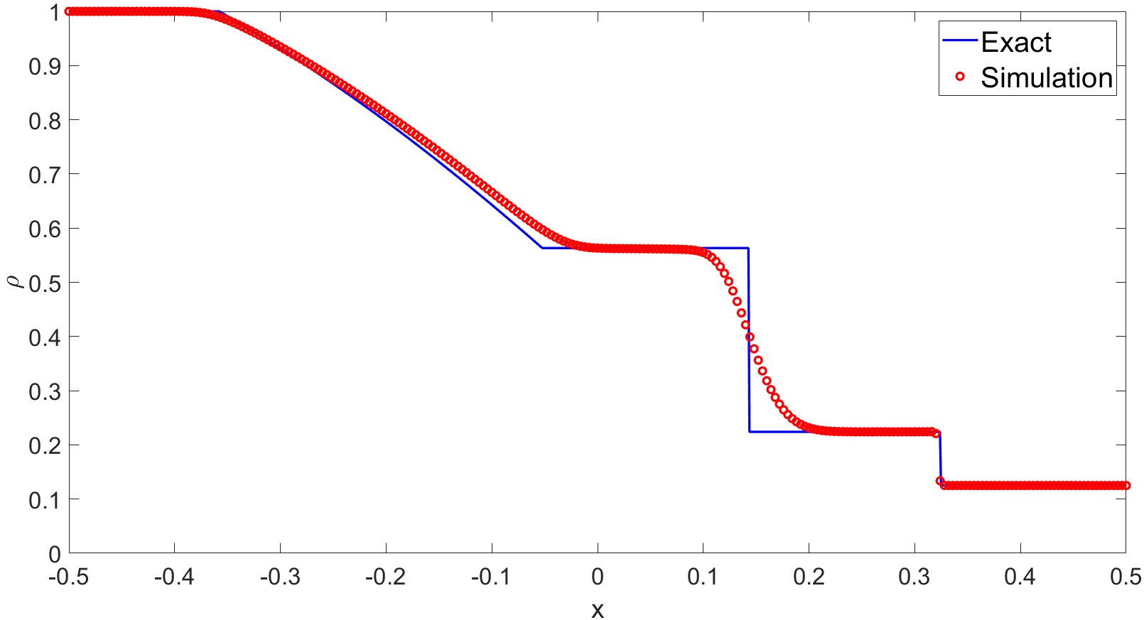
Refer to caption

a) Refer to caption b) Refer to caption c)

Figure 3: Sod shock tube problem with van der Waals EOS at t=0.2𝑡0.2t=0.2, comparison with exact solution, a) density, b) velocity, c) pressure.

Finally, we have analyzed the same test case for the Peng-Robinson EOS with a~=b~=0.5~𝑎~𝑏0.5\tilde{a}=\tilde{b}=0.5. In this case no analytic solution is available and a reference solution is computed using the third order optimal SSP Runge-Kutta method derived in [25] in combination with Q0subscript𝑄0Q_{0} finite elements and LLF as numerical flux on a mesh with 160001600016000 elements. Notice that, in the case of the van der Waals EOS, this procedure was found to provide a solution overlapping with the exact one. The good agreement between our numerical results and the reference ones is established also for this equation of state, as evident from Figure 4, again with significant smoothing of the contact discontinuity.
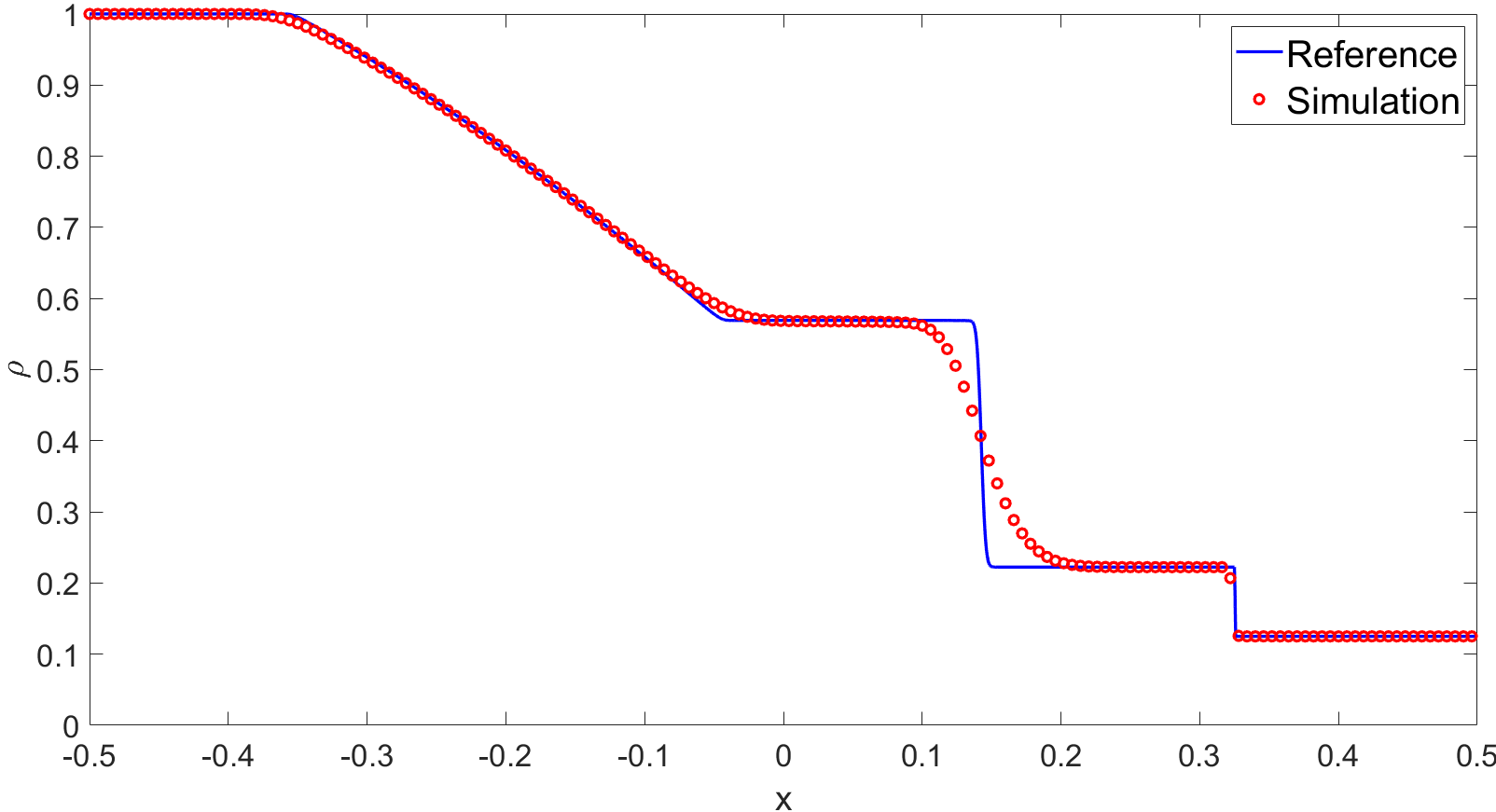
Refer to caption

a) Refer to caption b) Refer to caption c)

Figure 4: Sod shock tube problem with Peng-Robinson EOS at t=0.2𝑡0.2t=0.2, comparison with reference solution, a) density, b) velocity, c) pressure.

7.3 2D Lid-driven cavity

We consider now the classical 2D lid-driven cavity test case. The computational domain is the box Ω=(0,1)×(0,1)Ω0101\Omega=\left(0,1\right)\times\left(0,1\right) which is initialized with a density ρ=1𝜌1\rho=1 and a velocity 𝐮=𝟎𝐮0\mathbf{u}=\mathbf{0}. The flow is driven by the upper boundary, whose velocity is set to 𝐮=(1,0)T𝐮superscript10𝑇\mathbf{u}=\left(1,0\right)^{T}, while on the other three boundaries a no-slip condition is imposed. We set Re=100𝑅𝑒100Re=100 and M2=105superscript𝑀2superscript105M^{2}=10^{-5}. The advantage of the proposed scheme is that the allowed time step is more than 100 times larger than that of a fully explicit scheme. Indeed, the time-step chosen is such that the maximum advective Courant number Cusubscript𝐶𝑢C_{u} is around 0.120.120.12, while the maximum Courant number C𝐶C is around 494949. The streamlines are shown in Figure 5 and highlight the formation of the main recirculation pattern. A comparison of the horizontal component of the velocity along the vertical middle line and of the vertical component of the velocity along the horizontal middle line with the reference solutions in [20, 51] is also presented.
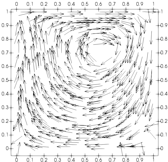
Refer to caption

a) Refer to caption b)

Figure 5: Computational results for the 2D lid-driven cavity, a) streamlines, b) comparison with the solutions in [20] and in [51]. Blue dots denote the results in [20], red crosses the results in [51] and the black line our numerical results.

We note a reasonable agreement between the different solutions, even though there is a still visible discrepancy between our results and the reference ones. Since the solution in [51] is obtained using third degree polynomials, in order to further improve the results, we consider also the case r=2𝑟2r=2. For this higher order approximation we note that our results fit very well both the reference solutions.
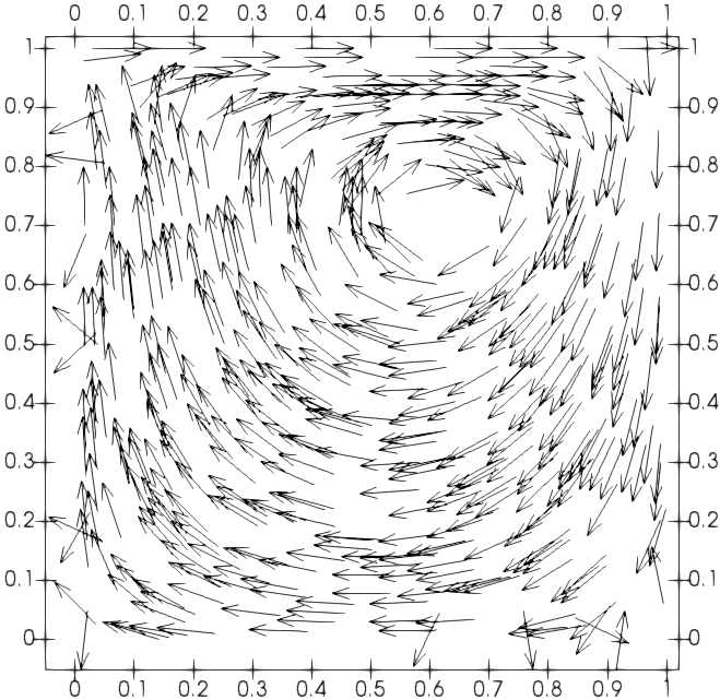
Refer to caption

a) Refer to caption b)

Figure 6: Computational results for the 2D lid-driven cavity with k=2𝑘2k=2, a) streamlines, b) comparison with the solutions in [20] and in [51]. Blue dots denote the results in [20], red crosses the results in [51] and black line our numerical results.

We have also tested the hlimit-fromh-adaptive version of the same algorithm, using a refinement criterion based on the vorticity. More specifically, we define

ηK=diam(K)2×𝐮2,K2subscript𝜂𝐾diamsuperscript𝐾2subscriptsuperscriptnorm𝐮22𝐾\eta_{K}=\text{diam}\left(K\right)^{2}\left\|\nabla\times\mathbf{u}\right\|^{2}_{2,K}

as local indicator. We start from a uniform Cartesian mesh with 161616 elements along each direction. We allowed refinement for 5%percent55\% of the elements with largest indicator values and coarsening for 30%percent3030\% of the elements with the smallest indicator values. The minimum element diameter allowed is =164164\mathcal{H}=\frac{1}{64}, while the maximum element diameter is =116116\mathcal{H}=\frac{1}{16}. Figure 7 reports the computational mesh at steady state and the computed streamlines. One can easily notice that the local refinement criterion is able to enhance automatically the resolution in the zones where vortices appear, as well as along the top boundary of the domain. For a more quantitative view, in Figure 8 we compare again the components of the velocity along the middle lines. Moreover, the absolute difference between the velocities of the fixed mesh and those of adaptive simulations is plotted over the whole domain, showing that no substantial loss of accuracy has occurred with a reduction of around 25% of the required computational time.
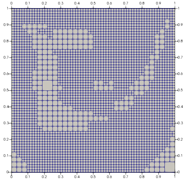
Refer to caption

a) Refer to caption b)

Figure 7: Adaptive simulation for the 2D lid-driven cavity, a) mesh at steady state, b) streamlines.
Refer to caption

a) Refer to caption b)

Figure 8: Adaptive simulation for the 2D lid-driven cavity, a) comparison with the solutions in [20] and in [51]. Blue dots denote the results in [20], red crosses the results in [51] and black line our numerical results, b) difference for velocity magnitude between the fixed grid simulation and the adaptive simulation (interpolated to the fixed grid).

7.4 Cold bubble

In this Section, we consider a test case proposed in [43, 44] for an ideal gas in which the gravity force is active. The computational domain is the rectangle (0,1000)×(0,2000)0100002000\left(0,1000\right)\times\left(0,2000\right) and the initial condition is represented by a thermal anomaly introduced in an isentropic background atmosphere with constant potential temperature θ0=303subscript𝜃0303\theta_{0}=303. The perturbation of potential temperature θsuperscript𝜃\theta^{{}^{\prime}} defines the initial datum and it is given by

θ={Aif r~r0Aexp((r~r0)2σ2)if r~>r0,superscript𝜃cases𝐴if ~𝑟subscript𝑟0𝐴superscript~𝑟subscript𝑟02superscript𝜎2if ~𝑟subscript𝑟0\theta^{{}^{\prime}}=\begin{cases}A&\text{if }\tilde{r}\leq r_{0}\\ A\exp\left(-\frac{\left(\tilde{r}-r_{0}\right)^{2}}{\sigma^{2}}\right)&\text{if }\tilde{r}>r_{0},\end{cases} (82)

with r~2=(xx0)2+(yy0)2superscript~𝑟2superscript𝑥subscript𝑥02superscript𝑦subscript𝑦02\tilde{r}^{2}=\left(x-x_{0}\right)^{2}+\left(y-y_{0}\right)^{2} and x0=500subscript𝑥0500x_{0}=500, y0=1250subscript𝑦01250y_{0}=1250, r0=50subscript𝑟050r_{0}=50, σ=100𝜎100\sigma=100 and A=15𝐴15A=-15. Moreover, we set Fr2=19.81,M2=105formulae-sequence𝐹superscript𝑟219.81superscript𝑀2superscript105Fr^{2}=\frac{1}{9.81},M^{2}=10^{-5} and Tf=50subscript𝑇𝑓50T_{f}=50. The expression of the Exner pressure is given by

Π=1M2Fr2yc~pθ,Π1superscript𝑀2𝐹superscript𝑟2𝑦subscript~𝑐𝑝𝜃\Pi=1-\frac{M^{2}}{Fr^{2}}\frac{y}{\tilde{c}_{p}\theta},

with y𝑦y denoting the vertical coordinate and c~p=γγ1R~g=1.0045102subscript~𝑐𝑝𝛾𝛾1subscript~𝑅𝑔1.0045superscript102\tilde{c}_{p}=\frac{\gamma}{\gamma-1}\tilde{R}_{g}=1.0045\cdot 10^{-2} denoting the non-dimensional specific heat at constant pressure. Notice that these values are obtained by considering =1 kg m3,𝒯𝒯=1 Kformulae-sequencetimes1timeskilogrammeter3𝒯𝒯times1kelvin\mathcal{R}=$1\text{\,}\mathrm{kg}\text{\,}{\mathrm{m}}^{-3}$,\mathcal{T}\mathcal{T}=$1\text{\,}\mathrm{K}$ and 𝒫=105 Pa𝒫superscript105timesabsentpascal{\mathcal{P}}=10^{5}\hskip 1.42271pt$\text{\,}\mathrm{Pa}$. Moreover, it is to be remarked that, unlike in [43], no artificial viscosity has been added to stabilize the computation. Wall boundary conditions are imposed at all the boundaries. The time step is taken to be Δt=0.08Δ𝑡0.08\Delta t=0.08, corresponding to a maximum Courant number C5.6𝐶5.6C\approx 5.6 and a maximum advective Courant number Cu0.18subscript𝐶𝑢0.18C_{u}\approx 0.18.

For the purpose of a quantitative comparison, a reference solution is computed with an explicit time discretization given by the optimal third order SSP scheme mentioned in Section 7.2. Figure 9 shows the contour plot of the potential temperature perturbation at t=Tf𝑡subscript𝑇𝑓t=T_{f} and one can easily notice that we are able to recover correctly the shape of the reference solution. For a more quantitative point of view, the profile of the density at y=1000𝑦1000y=1000 is reported in Figure 10 and a good agreement between the reference results and those obtained with the IMEX scheme is established. The IMEX scheme allows to employ a time step 404040 times larger compared to the fully explicit scheme with a computational saving of around 90%. Three fixed-point iterations were required on average for each IMEX stage.
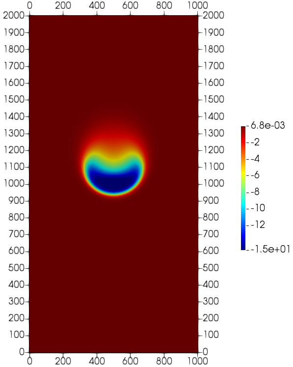
Refer to caption

a)

Refer to caption

b)

Figure 9: Cold bubble test case, results at t=Tf𝑡subscript𝑇𝑓t=T_{f}, a) contour plot of potential temperature perturbation for the reference explicit simulation, b) contour plot of the potential temperature perturbation for the simulation with IMEX scheme.
Refer to caption
Figure 10: Cold bubble test case, results at t=Tf𝑡subscript𝑇𝑓t=T_{f}, density profile at y=1000𝑦1000y=1000. The continuous blue line represents the results for the reference explicit simulation, whereas the red dots denote the results for the IMEX scheme.

In order to further enhance the computational efficiency, we employ again the code hlimit-fromh-adaptivity capabilities. As mentioned in Section 3, we use as refinement indicator the gradient of the potential temperature, since this quantity allows to identify the cold bubble. More specifically, we set

ηK=maxi𝒩K|θ|isubscript𝜂𝐾subscript𝑖subscript𝒩𝐾subscript𝜃𝑖\eta_{K}=\max_{i\in\mathcal{N}_{K}}\left|\nabla\theta\right|_{i} (83)

as local indicator, where 𝒩Ksubscript𝒩𝐾\mathcal{N}_{K} is defined as in (81), and we allow to refine when ηKsubscript𝜂𝐾\eta_{K} exceeds 101superscript10110^{-1} and to coarsen below 61026superscript1026\cdot 10^{-2}. The initial computational grid is composed by 50×1005010050\times 100 elements and we allow up to two local refinements only, so as to keep the advective Courant number under control and to recover the same maximum resolution employed for the non adaptive mesh simulation. As one can easily notice from Figure 11, the refinement criterion is able to track the bubble and the one-dimensional density profile at y=1000𝑦1000y=1000 in Figure 12 is correctly reproduced. The final mesh consists of 6914 elements instead of the 80000 elements of the full resolution mesh and a further 50% reduction in computational time is achieved.
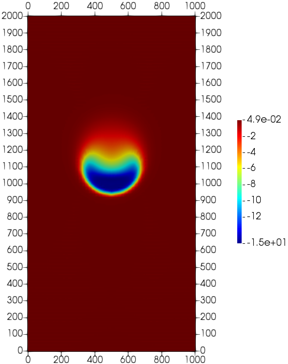
Refer to caption

a)

Refer to caption

b)

Figure 11: Cold bubble test case, adaptive simulation, results at t=Tf𝑡subscript𝑇𝑓t=T_{f}, a) contour plot of potential temperature perturbation, b) computational grid.
Refer to caption
Figure 12: Cold bubble test case, adaptive simulation, results at t=Tf𝑡subscript𝑇𝑓t=T_{f}, density profile at y=1000𝑦1000y=1000. The continuous blue line represents the results for the reference explicit simulation, whereas the red dots denote the results for the IMEX scheme.

We repeat now the same test using non-ideal equations of state. We first consider the van der Waals equation with a constant c~vsubscript~𝑐𝑣\tilde{c}_{v} given by c~v=R~gγ1=7.175103,a~=5109formulae-sequencesubscript~𝑐𝑣subscript~𝑅𝑔𝛾17.175superscript103~𝑎5superscript109\tilde{c}_{v}=\frac{\tilde{R}_{g}}{\gamma-1}=7.175\cdot 10^{-3},\tilde{a}=5\cdot 10^{-9} and b~=5104~𝑏5superscript104\tilde{b}=5\cdot 10^{-4}, so that the same specific heat at constant volume with respect to the ideal gas case is obtained and z1𝑧1z\approx 1. The fluid is initialized using the same pressure and the same density values as in the ideal gas case. Notice that da~dT=dc~vdT=0𝑑~𝑎𝑑𝑇𝑑subscript~𝑐𝑣𝑑𝑇0\frac{d\tilde{a}}{dT}=\frac{d\tilde{c}_{v}}{dT}=0 and so it is not necessary to explicitly compute the temperature for (4) and (4). We expect a behaviour similar to the ideal gas one and this is confirmed by the density profile reported in Figure 13.

Refer to caption
Figure 13: Cold bubble test case, van der Waals EOS with a~=5109~𝑎5superscript109\tilde{a}=5\cdot 10^{-9} and b~=5104~𝑏5superscript104\tilde{b}=5\cdot 10^{-4}, results at t=Tf𝑡subscript𝑇𝑓t=T_{f}, density profile at y=1000𝑦1000y=1000. The continuous blue line represents the results for the reference explicit simulation, whereas the red dots denote the results for the IMEX scheme.

We then consider the case with a~=1.6101~𝑎1.6superscript101\tilde{a}=1.6\cdot 10^{-1} and b~=5104~𝑏5superscript104\tilde{b}=5\cdot 10^{-4}, which yield an average compressibility factor z0.83𝑧0.83z\approx 0.83. In this case, we expect effects due to conditions far from the ideal ones and so we first compute a reference solution with the explicit time discretization. The time step for the IMEX simulation is kept equal to Δt=0.08Δ𝑡0.08\Delta t=0.08, yielding a maximum Courant number C5.3𝐶5.3C\approx 5.3 and a maximum advective Courant number Cu0.19subscript𝐶𝑢0.19C_{u}\approx 0.19. Figure 14 shows the contour plot for β𝛽\beta at t=Tf𝑡subscript𝑇𝑓t=T_{f} for both the reference explicit and the IMEX simulations. The expected behaviour is retrieved and a good agreement with the reference results is established. Also in this case, a computational saving of around 90% with respect to the explicit simulation is obtained thanks to the IMEX scheme. Figure 15 reports the profile of the density for y=1000𝑦1000y=1000 at t=Tf𝑡subscript𝑇𝑓t=T_{f}. One can notice the very good agreement between the IMEX results and the reference ones. Furthermore, a clear discrepancy with respect to the ideal gas can be observed. The higher density values are due to the large value of a~~𝑎\tilde{a}, which means that strong forces of attraction between the gas particles are present [39].

Refer to caption

a)

Refer to caption

b)

Figure 14: Cold bubble test case, van der Waals EOS with a~=1.6101~𝑎1.6superscript101\tilde{a}=1.6\cdot 10^{-1} and b~=5104~𝑏5superscript104\tilde{b}=5\cdot 10^{-4}, results at t=Tf𝑡subscript𝑇𝑓t=T_{f}, a) contour plot of β𝛽\beta for the reference explicit simulation, b) contour plot of β𝛽\beta for the simulation with IMEX scheme.
Refer to caption
Figure 15: Cold bubble test case, van der Waals EOS with a~=1.6101~𝑎1.6superscript101\tilde{a}=1.6\cdot 10^{-1} and b~=5104~𝑏5superscript104\tilde{b}=5\cdot 10^{-4}, results at t=Tf𝑡subscript𝑇𝑓t=T_{f}, density profile at y=1000𝑦1000y=1000. The continuous blue line represents the results for the full explicit simulation, the continuous black line reports the results for the reference explicit simulation with an ideal gas, whereas the red dots denote the results for the IMEX scheme.

Concerning the adaptive simulations, since, as proven in Section 3, the quantity β=log(T)2R~gc~vatanh(2ρb~1)𝛽𝑇2subscript~𝑅𝑔subscript~𝑐𝑣atanh2𝜌~𝑏1\beta=\log(T)-2\frac{\tilde{R}_{g}}{\tilde{c}_{v}}\operatorname{atanh}\left(2\rho\tilde{b}-1\right) is constant in an isentropic process with da~dT=dc~vdT=0𝑑~𝑎𝑑𝑇𝑑subscript~𝑐𝑣𝑑𝑇0\frac{d\tilde{a}}{dT}=\frac{d\tilde{c}_{v}}{dT}=0, we define the local refinement indicator for each element as

ηK=maxi𝒩K|β|i.subscript𝜂𝐾subscript𝑖subscript𝒩𝐾subscript𝛽𝑖\eta_{K}=\max_{i\in\mathcal{N}_{K}}\left|\nabla\beta\right|_{i}. (84)

We allow to refine when ηKsubscript𝜂𝐾\eta_{K} exceeds 41044superscript1044\cdot 10^{-4} and to coarsen when the indicator is below 21042superscript1042\cdot 10^{-4}. The initial mesh is composed by 50×1005010050\times 100 elements and we allow up to four local refinements. For this reason, in order to keep under control the advective Courant number, we need to reduce the time step Δt=0.02Δ𝑡0.02\Delta t=0.02, so as to obtain a maximum acoustic Courant number C5.3𝐶5.3C\approx 5.3 and a maximum advective Courant number Cu0.18subscript𝐶𝑢0.18C_{u}\approx 0.18. Figure 16 confirms that β𝛽\beta is an appropriate quantity to track the bubble and the one-dimensional density profile in Figure 17 shows that no significant loss in accuracy occurs. The final mesh consists of 9086 elements.

Refer to caption

a)

Refer to caption

b)

Figure 16: Cold bubble test case, van der Waals EOS with a~=1.6101~𝑎1.6superscript101\tilde{a}=1.6\cdot 10^{-1} and b~=5104~𝑏5superscript104\tilde{b}=5\cdot 10^{-4}, adaptive simulation, results at t=Tf𝑡subscript𝑇𝑓t=T_{f}, a) contour plot of β𝛽\beta, b) computational grid.
Refer to caption
Figure 17: Cold bubble test case, van der Waals EOS with a~=1.6101~𝑎1.6superscript101\tilde{a}=1.6\cdot 10^{-1} and b~=5104~𝑏5superscript104\tilde{b}=5\cdot 10^{-4}, adaptive simulation, results at t=Tf𝑡subscript𝑇𝑓t=T_{f}, density profile at y=1000𝑦1000y=1000. The continuous blue line represents the results for the reference explicit simulation, the continuous black line reports the results for the reference explicit simulation with an ideal gas, whereas the red dots denote the results for the IMEX scheme in the non-ideal case.

The same analysis is carried out using the Peng-Robinson EOS. Hence, we first consider R~g=2.87103subscript~𝑅𝑔2.87superscript103\tilde{R}_{g}=2.87\cdot 10^{-3}, c~v=7.175103subscript~𝑐𝑣7.175superscript103\tilde{c}_{v}=7.175\cdot 10^{-3}, a~=5109~𝑎5superscript109\tilde{a}=5\cdot 10^{-9} and b~=5104~𝑏5superscript104\tilde{b}=5\cdot 10^{-4}, so that z1𝑧1z\approx 1. The density profile reported in Figure 18 highlights, as expected, a behaviour entirely analogous to that of the ideal gas.
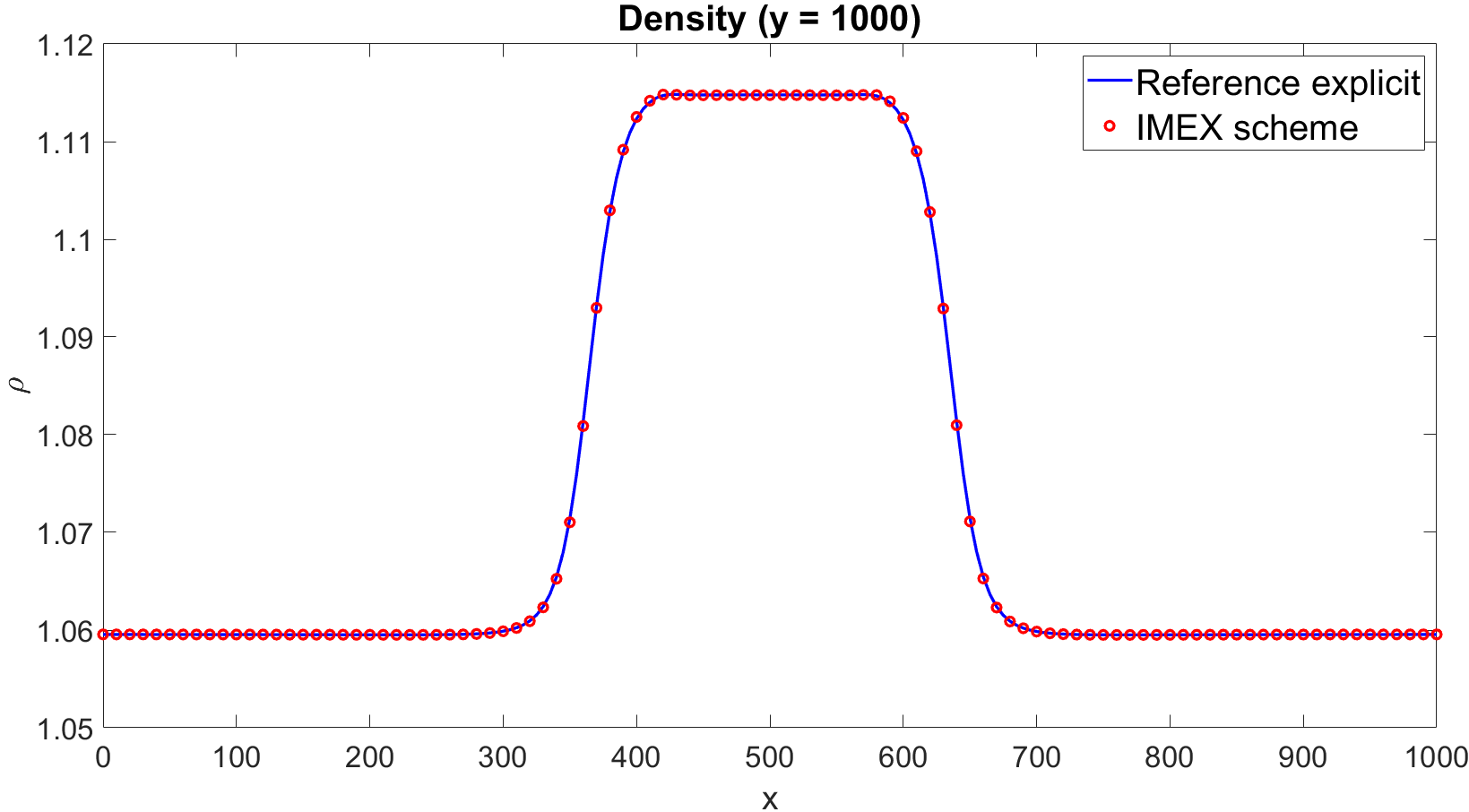
Refer to caption
Figure 18: Cold bubble test case, Peng-Robinson EOS with a~=5109~𝑎5superscript109\tilde{a}=5\cdot 10^{-9} and b~=5104~𝑏5superscript104\tilde{b}=5\cdot 10^{-4}, results at t=Tf𝑡subscript𝑇𝑓t=T_{f}, density profile at y=1000𝑦1000y=1000. The continuous blue line represents the results for the reference explicit simulation, whereas the red dots denote the results for the IMEX scheme.

Next, we take a~=1.6101~𝑎1.6superscript101\tilde{a}=1.6\cdot 10^{-1} and b~=5104~𝑏5superscript104\tilde{b}=5\cdot 10^{-4}, so that z0.83𝑧0.83z\approx 0.83, and we perform both uniform mesh and adaptive simulations, using the same parameters employed for the van der Waals EOS. The results are compared with a reference solution computed with the explicit method. Figure 19 shows similar contour plots for all the configurations as well as for the adaptive mesh at t=Tf𝑡subscript𝑇𝑓t=T_{f}, which consists of 913791379137 elements and it is able to track the bubble correctly. Figure 20 reports the comparison for the one-dimensional profile of the density at y=1000𝑦1000y=1000 and the same considerations of the van der Waals EOS are still valid. We want to test in this case the refinement indicator based on (35). More specifically, we set

ηK=maxi𝒩K|(pργpρ)|isubscript𝜂𝐾subscript𝑖subscript𝒩𝐾subscript𝑝superscript𝜌subscript𝛾𝑝𝜌𝑖\eta_{K}=\max_{i\in\mathcal{N}_{K}}\left|\nabla\left(\frac{p}{\rho^{\gamma_{p\rho}}}\right)\right|_{i} (85)

and we allow to refine in case ηKsubscript𝜂𝐾\eta_{K} is above 41044superscript1044\cdot 10^{-4} and to coarsen below 21042superscript1042\cdot 10^{-4} with the same remeshing procedure adopted so far for non-ideal gases. Figure 21 shows the contour plot of (35) and the computational mesh at t=Tf𝑡subscript𝑇𝑓t=T_{f}. The mesh consists of 829482948294 elements and one can easily notice that more resolution is added only in correspondence of the bubble.
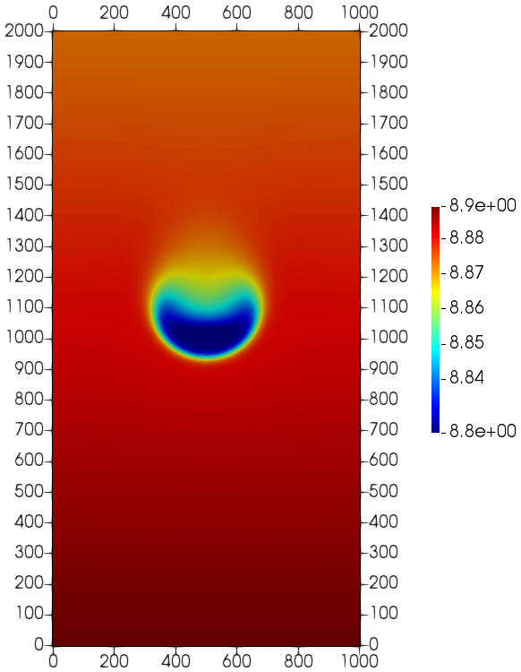
Refer to caption

a)

Refer to caption

b)

Refer to caption

a)

Refer to caption

b)

Figure 19: Cold bubble test case, Peng-Robinson EOS with a~=1.6101~𝑎1.6superscript101\tilde{a}=1.6\cdot 10^{-1} and b~=5104~𝑏5superscript104\tilde{b}=5\cdot 10^{-4}, results at t=Tf𝑡subscript𝑇𝑓t=T_{f}, a) contour plot of β𝛽\beta for the reference explicit simulation, b) contour plot of β𝛽\beta for the constant mesh simulation with IMEX scheme, c) contour plot of β𝛽\beta for adaptive simulation with IMEX scheme, d) adaptive mesh.
Refer to caption
Figure 20: Cold bubble test case, Peng-Robinson EOS with a~=1.6101~𝑎1.6superscript101\tilde{a}=1.6\cdot 10^{-1} and b~=5104~𝑏5superscript104\tilde{b}=5\cdot 10^{-4}, adaptive simulation, results at t=Tf𝑡subscript𝑇𝑓t=T_{f}, density profile at y=1000𝑦1000y=1000. The continuous blue line represents the results for the reference explicit simulation, the continuous black line reports the results for the reference explicit simulation with an ideal gas, the red dots denote the results for the IMEX scheme, whereas the green squares represent the results for the adaptive simulation with IMEX scheme.
Refer to caption

a)

Refer to caption

b)

Figure 21: Cold bubble test case, Peng-Robinson EOS with a~=1.6101~𝑎1.6superscript101\tilde{a}=1.6\cdot 10^{-1} and b~=5104~𝑏5superscript104\tilde{b}=5\cdot 10^{-4}, adaptive simulation with criterion (85), results at t=Tf𝑡subscript𝑇𝑓t=T_{f}, a) contour plot of (35), b) adaptive mesh

7.5 Warm bubble

In order to test the method in presence of heat conduction, we now consider for an ideal gas the test case of a rising warm bubble proposed in [11]. The domain is the square box Ω=(0.5,1.5)×(0.5,1.5)Ω0.51.50.51.5\Omega=\left(-0.5,1.5\right)\times\left(-0.5,1.5\right) with periodic boundary conditions on the lateral boundaries and wall boundary conditions on the top and on the bottom of the domain. The initial temperature corresponds to a truncated Gaussian profile

T(𝐱,0)={386.48if r~>r0p~0R~g,air(10.1er~2σ2)if r~r0,𝑇𝐱0cases386.48if ~𝑟subscript𝑟0subscript~𝑝0subscript~𝑅𝑔𝑎𝑖𝑟10.1superscript𝑒superscript~𝑟2superscript𝜎2if ~𝑟subscript𝑟0T(\mathbf{x},0)=\begin{cases}386.48\qquad&\text{if }\tilde{r}>r_{0}\\ \frac{\tilde{p}_{0}}{\tilde{R}_{g,air}\left(1-0.1e^{\frac{\tilde{r}^{2}}{\sigma^{2}}}\right)}\qquad&\text{if }\tilde{r}\leq r_{0},\end{cases} (86)

where r~2=(xx0)2+(yy0)2superscript~𝑟2superscript𝑥subscript𝑥02superscript𝑦subscript𝑦02\tilde{r}^{2}=\left(x-x_{0}\right)^{2}+\left(y-y_{0}\right)^{2} is the distance from the center with coordinates x0=0.5subscript𝑥00.5x_{0}=0.5 and y0=0.35subscript𝑦00.35y_{0}=0.35, r0=0.25subscript𝑟00.25r_{0}=0.25 is the radius and σ=2𝜎2\sigma=2. In this Section, we consider unitary reference values for density, pressure and temperature and, therefore, we set p~0=105subscript~𝑝0superscript105\tilde{p}_{0}=10^{5} and R~g,air=287subscript~𝑅𝑔𝑎𝑖𝑟287\tilde{R}_{g,air}=287. Moreover, following [11], we consider:

Re=804.9Pr=0.71Fr0.004M0.01.formulae-sequence𝑅𝑒804.9formulae-sequence𝑃𝑟0.71formulae-sequence𝐹𝑟0.004𝑀0.01Re=804.9\qquad Pr=0.71\qquad Fr\approx 0.004\qquad M\approx 0.01.

The grid is composed by 120 elements along each direction and the time step is such that the maximum Courant number C118𝐶118C\approx 118 and the maximum value of advective Courant number Cusubscript𝐶𝑢C_{u} is around 0.030.030.03. Figures 22, 23 and 24 show the results at t=10,15,20 s𝑡101520timesabsentsecondt=10,15,20\hskip 1.42271pt$\text{\,}\mathrm{s}$ both in terms of contours and plots along the same specific sections along xlimit-from𝑥x-axis chosen in [11]. All the results are in good agreement with the reference ones and we are able to recover the development of the expected Kelvin-Helmholtz instability.
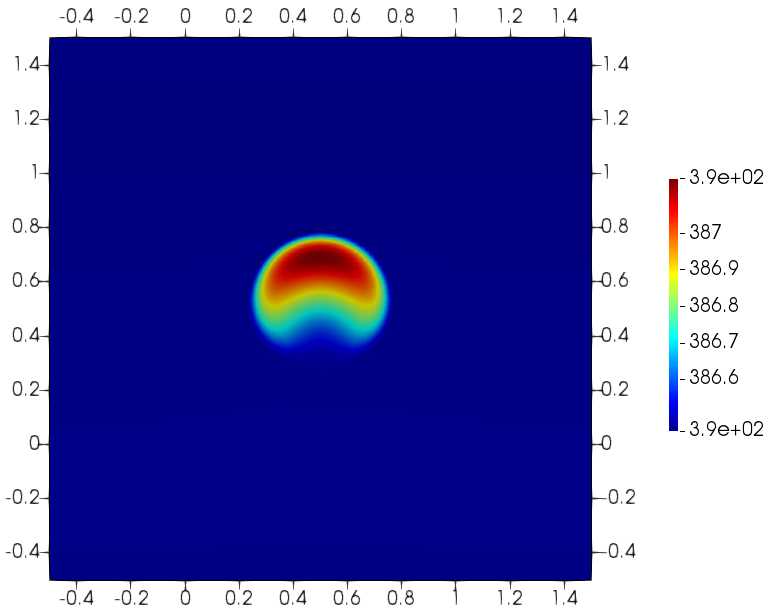
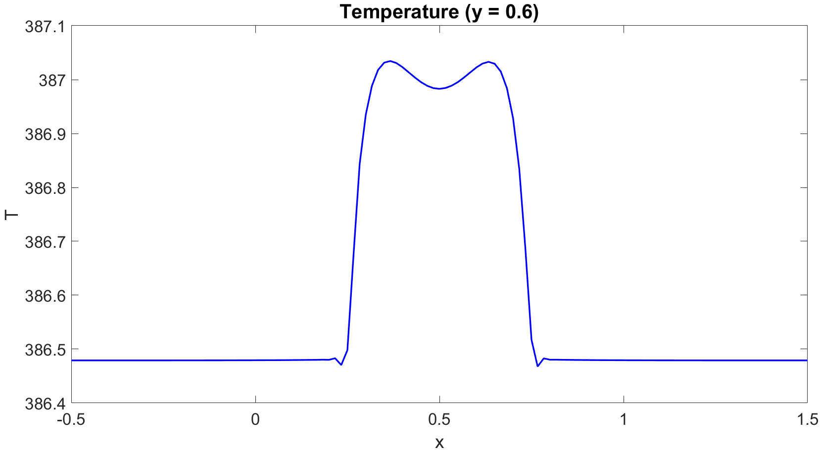
Refer to caption
Refer to caption
Refer to caption
Refer to caption
Refer to caption
Refer to caption
Figure 22: Warm bubble test case, results at t=10 s𝑡times10secondt=$10\text{\,}\mathrm{s}$. From bottom to top: temperature, horizontal velocity and vertical velocity.
Refer to caption
Refer to caption
Refer to caption
Refer to caption
Refer to caption
Refer to caption
Figure 23: Warm bubble test case, results at t=15 s𝑡times15secondt=$15\text{\,}\mathrm{s}$. From bottom to top: temperature, horizontal velocity and vertical velocity.
Refer to caption
Refer to caption
Refer to caption
Refer to caption
Refer to caption
Refer to caption
Figure 24: Warm bubble test case, results at t=20 s𝑡times20secondt=$20\text{\,}\mathrm{s}$. From bottom to top: temperature, horizontal velocity and vertical velocity.

The same test is repeated using data for nitrous oxide (N2O)subscript𝑁2𝑂\left(N_{2}O\right) from [37], which we report here for the convenience of the reader. At temperature of 386.48 Ktimes386.48kelvin386.48\text{\,}\mathrm{K} and pressure of 105 Pasuperscript105timesabsentpascal10^{5}\hskip 1.42271pt$\text{\,}\mathrm{Pa}$, μ=1.8884105 Pas𝜇1.8884superscript105timesabsentPas\mu=1.8884\cdot 10^{-5}\hskip 1.42271pt$\text{\,}\mathrm{Pa}\cdot\mathrm{s}$ and κ=2.4855102 W m1 K1𝜅2.4855superscript102timesabsenttimeswattmeter1kelvin1\kappa=2.4855\cdot 10^{-2}\hskip 1.42271pt$\text{\,}\mathrm{W}\text{\,}{\mathrm{m}}^{-1}\text{\,}{\mathrm{K}}^{-1}$, so as to obtain

Re716.1Pr0.73.formulae-sequence𝑅𝑒716.1𝑃𝑟0.73Re\approx 716.1\qquad Pr\approx 0.73.

We consider the Peng-Robinson EOS, for which the expressions of a~(T)~𝑎𝑇\tilde{a}(T) and b~~𝑏\tilde{b} are the following [17]:

{a~(T)=0.45724R~g2T~c2p~cα(T)2α(T)=1+Γ(1TT~c)Γ=0.37464+1.54226ω0.26992ω2b~=0.0778R~gT~cp~c,cases~𝑎𝑇absent0.45724superscriptsubscript~𝑅𝑔2superscriptsubscript~𝑇𝑐2subscript~𝑝𝑐𝛼superscript𝑇2𝛼𝑇absent1Γ1𝑇subscript~𝑇𝑐Γabsent0.374641.54226𝜔0.26992superscript𝜔2~𝑏absent0.0778subscript~𝑅𝑔subscript~𝑇𝑐subscript~𝑝𝑐\begin{cases}\tilde{a}(T)&=0.45724\frac{\tilde{R}_{g}^{2}\tilde{T}_{c}^{2}}{\tilde{p}_{c}}\alpha(T)^{2}\\ \alpha(T)&=1+\Gamma\left(1-\sqrt{\frac{T}{\tilde{T}_{c}}}\right)\\ \Gamma&=0.37464+1.54226\omega-0.26992\omega^{2}\\ \tilde{b}&=0.0778\frac{\tilde{R}_{g}\tilde{T}_{c}}{\tilde{p}_{c}},\end{cases} (87)

where T~csubscript~𝑇𝑐\tilde{T}_{c} denotes the non-dimensional critical temperature, p~csubscript~𝑝𝑐\tilde{p}_{c} the non-dimensional critical pressure and ω𝜔\omega the acentric factor. For what concerns N2Osubscript𝑁2𝑂N_{2}O, we find from [37] T~c=309.52,p~c=7.2450106formulae-sequencesubscript~𝑇𝑐309.52subscript~𝑝𝑐7.2450superscript106\tilde{T}_{c}=309.52,\tilde{p}_{c}=7.2450\cdot 10^{6} and ω=0.1613𝜔0.1613\omega=0.1613. Finally, the function c~v(T)subscript~𝑐𝑣𝑇\tilde{c}_{v}(T) is computed using the following polynomial from [37]:

c~v(T)subscript~𝑐𝑣𝑇\displaystyle\tilde{c}_{v}\left(T\right) =\displaystyle= 1T[[AT1000+12B(T1000)2+13C(T1000)3+\displaystyle\frac{1}{T}\left[\left[A\frac{T}{1000}+\frac{1}{2}B\left(\frac{T}{1000}\right)^{2}+\frac{1}{3}C\left(\frac{T}{1000}\right)^{3}+\right.\right. (88)
14D(T1000)4E1000T]106MwR~g,N2OT],\displaystyle\hskip 21.33955pt\left.\left.\frac{1}{4}D\left(\frac{T}{1000}\right)^{4}-E\frac{1000}{T}\right]\frac{10^{6}}{M_{w}}-\tilde{R}_{g,N_{2}O}T\right],

with R~g,N2O=188.91subscript~𝑅𝑔subscript𝑁2𝑂188.91\tilde{R}_{g,N_{2}O}=188.91, Mw=44.0128subscript𝑀𝑤44.0128M_{w}=44.0128 and A,B,C,D,E𝐴𝐵𝐶𝐷𝐸A,B,C,D,E denoting suitable coefficients whose values are reported in Table 19. It is worth to mention once more that c~v(T)subscript~𝑐𝑣𝑇\tilde{c}_{v}(T) is not a proper specific heat at constant volume, but it denotes the non-dimensional counterpart of e#(T)Tsuperscript𝑒#𝑇𝑇\frac{e^{\#}(T)}{T} from (10), as shown in (16). The fluid is initialized with the same temperature and the same pressure as the ideal gas. The same mesh and the time step of the previous case are used, yielding to C92𝐶92C\approx 92 and Cu0.03subscript𝐶𝑢0.03C_{u}\approx 0.03. Figure 25 shows the temperature, the horizontal and the vertical velocity at t=20 s𝑡times20secondt=$20\text{\,}\mathrm{s}$. One can easily notice that a good qualitative agreement compared with the results in Figure 24 is obtained. For a more quantitative point of view, since an explicit solution cannot be computed in view of the very large acoustic Courant number and the compressibility factor is z0.997𝑧0.997z\approx 0.997, a simulation with the ideal gas law (28) is performed, using γ=1.2879𝛾1.2879\gamma=1.2879, which corresponds to c~v(386.48)R~g+1subscript~𝑐𝑣386.48subscript~𝑅𝑔1\frac{\tilde{c}_{v}\left(386.48\right)}{\tilde{R}_{g}}+1, so that the internal energy of the ideal gas at T=386.48𝑇386.48T=386.48 is the same as in the case e#(386.48)superscript𝑒#386.48e^{\#}\left(386.48\right). The temperature profile at y=0.8𝑦0.8y=0.8 shown in Figure 26 confirms the good quality of the solution, with only slight differences due to the different equations of state.
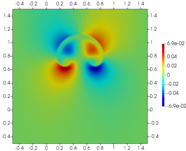
A𝐴A 27.6798827.6798827.67988
B𝐵B 51.1489851.1489851.14898
C𝐶C 30.6454430.64544-30.64544
D𝐷D 6.8479116.8479116.847911
E𝐸E 0.1579060.157906-0.157906
Table 19: Values for polynomial (88)
Refer to caption

a)

Refer to caption

b)

Refer to caption

c)

Figure 25: Warm bubble test case for N2Osubscript𝑁2𝑂N_{2}O with Peng-Robinson EOS, results at t=20 s𝑡times20secondt=$20\text{\,}\mathrm{s}$, a) horizontal velocity, b) vertical velocity, c) temperature.
Refer to caption
Figure 26: Warm bubble test case for N2Osubscript𝑁2𝑂N_{2}O with Peng-Robinson EOS, temperature profile for y=0.8𝑦0.8y=0.8 at t=20 s𝑡times20secondt=$20\text{\,}\mathrm{s}$.

In order to consider also non-ideal effects, we focus on conditions closer to the vapor-liquid phase equilibrium conditions, which are definitely more challenging. More in detail, we set p=4106𝑝4superscript106p=4\cdot 10^{6} and we consider the following temperature profile

T(𝐱,0)={298if r~>r0p~0R~g,air(10.1er~2σ2)88.48if r~r0,𝑇𝐱0cases298if ~𝑟subscript𝑟0subscript~𝑝0subscript~𝑅𝑔𝑎𝑖𝑟10.1superscript𝑒superscript~𝑟2superscript𝜎288.48if ~𝑟subscript𝑟0T(\mathbf{x},0)=\begin{cases}298\qquad&\text{if }\tilde{r}>r_{0}\\ \frac{\tilde{p}_{0}}{\tilde{R}_{g,air}\left(1-0.1e^{\frac{\tilde{r}^{2}}{\sigma^{2}}}\right)}-88.48\qquad&\text{if }\tilde{r}\leq r_{0},\end{cases} (89)

which corresponds to a translation with respect to (86), yielding z0.72𝑧0.72z\approx 0.72. We would like to point out that these conditions of pressure and temperature are close to the vapour-liquid phase transition curve of N2Osubscript𝑁2𝑂N_{2}O. The maximum acoustic Courant is C74.5𝐶74.5C\approx 74.5, whereas the maximum advective Courant number is Cu0.06subscript𝐶𝑢0.06C_{u}\approx 0.06. Figure 27 shows the contour plots of the temperature at t=15 s𝑡times15secondt=$15\text{\,}\mathrm{s}$ and t=20 s𝑡times20secondt=$20\text{\,}\mathrm{s}$. For these conditions of temperature and pressure, we obtain from [37] μ=1.6680105 Pas𝜇1.6680superscript105timesabsentPas\mu=1.6680\cdot 10^{-5}\hskip 1.42271pt$\text{\,}\mathrm{Pa}\cdot\mathrm{s}$, κ=2.1201102 W m1 K1𝜅2.1201superscript102timesabsenttimeswattmeter1kelvin1\kappa=2.1201\cdot 10^{-2}\hskip 1.42271pt$\text{\,}\mathrm{W}\text{\,}{\mathrm{m}}^{-1}\text{\,}{\mathrm{K}}^{-1}$ and cp=1.5150103 J kg1 K1subscript𝑐𝑝1.5150superscript103timesabsenttimesjoulekilogram1kelvin1c_{p}=1.5150\cdot 10^{3}\hskip 1.42271pt$\text{\,}\mathrm{J}\text{\,}{\mathrm{kg}}^{-1}\text{\,}{\mathrm{K}}^{-1}$, so as to obtain

Re810.7Pr1.19formulae-sequence𝑅𝑒810.7𝑃𝑟1.19Re\approx 810.7\quad Pr\approx 1.19

One can easily notice the full development of the Kelvin-Helmholtz instability with the formation of secondary vortices. The bubble reaches a higher altitude with respect to the previous case.
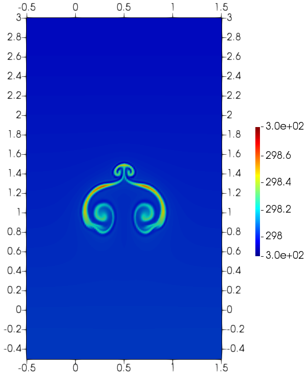
Refer to caption

a)

Refer to caption

b)

Figure 27: Warm bubble test case for N2Osubscript𝑁2𝑂N_{2}O with Peng-Robinson EOS, a) temperature at t=15 s𝑡times15secondt=$15\text{\,}\mathrm{s}$, b) temperature at t=20 s𝑡times20secondt=$20\text{\,}\mathrm{s}$.
Refer to caption

a)

Refer to caption

b)

Figure 28: Warm bubble test case for N2Osubscript𝑁2𝑂N_{2}O with Peng-Robinson EOS, a) vertical velocity at t=15 s𝑡times15secondt=$15\text{\,}\mathrm{s}$, b) vertical velocity at t=20 s𝑡times20secondt=$20\text{\,}\mathrm{s}$.

Finally, we consider the SG-EOS with γ=1.0936,c~v=1453.91formulae-sequence𝛾1.0936subscript~𝑐𝑣1453.91\gamma=1.0936,\tilde{c}_{v}=1453.91 and π~=q~=0~𝜋~𝑞0\tilde{\pi}=\tilde{q}=0. The values for γ𝛾\gamma and c~vsubscript~𝑐𝑣\tilde{c}_{v} are computed using the procedure described in [19]. The maximum acoustic Courant is C67𝐶67C\approx 67, whereas the maximum advective Courant number is Cu0.04subscript𝐶𝑢0.04C_{u}\approx 0.04. Figure 29 shows the contour plots of the temperature at t=15 s𝑡times15secondt=$15\text{\,}\mathrm{s}$ and t=20 s𝑡times20secondt=$20\text{\,}\mathrm{s}$. The different behaviour between the two equations of state can be readily explained since, in the case of Peng-Robinson EOS, the difference between the density of the bubble and the background density is bigger with respect to SG-EOS, as evident from Figure 31 and, therefore, a bigger upward buoyant force is exerted on the bubble. For this reason, in the simulation with Peng-Robinson EOS reaches a higher level compared to that in the SG-EOS simulation.
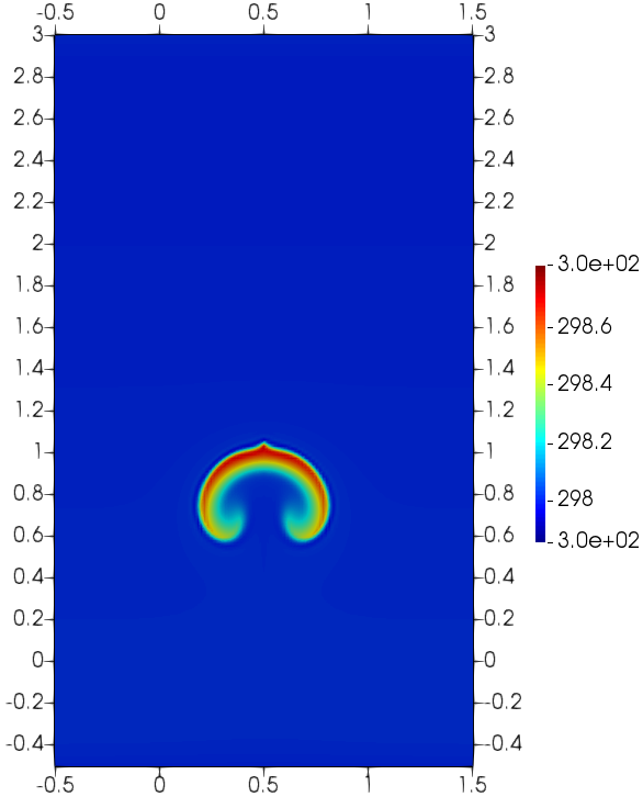
Refer to caption

a)

Refer to caption

b)

Figure 29: Warm bubble test case for N2Osubscript𝑁2𝑂N_{2}O with SG-EOS, a) temperature at t=15 s𝑡times15secondt=$15\text{\,}\mathrm{s}$, b) temperature at t=20 s𝑡times20secondt=$20\text{\,}\mathrm{s}$.
Refer to caption

a)

Refer to caption

b)

Figure 30: Warm bubble test case for N2Osubscript𝑁2𝑂N_{2}O with SG-EOS, a) vertical velocity at t=15 s𝑡times15secondt=$15\text{\,}\mathrm{s}$, b) vertical velocity at t=20 s𝑡times20secondt=$20\text{\,}\mathrm{s}$.
Refer to caption

a)

Refer to caption

b)

Figure 31: Warm bubble test case for N2Osubscript𝑁2𝑂N_{2}O, density deviation from background state at t=0𝑡0t=0, a) Peng-Robinson EOS, b) SG-EOS.

8 Conclusions and future perspectives

We have proposed an efficient, hlimit-fromh-adaptive IMEX-DG solver for the compressible Navier-Stokes equations with non-ideal EOS. The solver combines ideas from the discretization approaches in [12, 14, 23, 33] and proposes an improvement in the choice of the free parameter employed by the explicit part of the IMEX scheme described in [23]. The resulting method achieves full second order accuracy also including viscous terms and implements an hlimit-fromh-adaptive approach in the framework of the numerical library deal.II. A number of physically based adaptation criteria have been proposed, which allow to exploit the full efficiency of the adaptive technique also for non-ideal gas simulations. A number of numerical experiments validate the proposed method and show its potential for low Mach number problems. In future work, we plan to extend the scheme to multiphase flows and to demonstrate its potential for application to atmospheric flows.

Acknowledgements

We thank M. Tavelli for providing the original data of the cavity flow simulation discussed in Section 7. We also gratefully acknowledge several useful discussions with A. Della Rocca on numerical methods related to those presented here. The simulations have been partly run at CINECA thanks to the computational resources made available through the SIDICoNS - HP10CLPLXI ISCRA-C project.

Appendix A Stability and monotonicity of the explicit time discretization

In this Appendix, we study the stability and monotonicity of the explicit part of the IMEX scheme applied in the paper. We recall that the Butcher tableaux for the explicit part of the method is given by

0 0
γ𝛾\gamma γ𝛾\gamma 0
1 1α1𝛼1-\alpha α𝛼\alpha 0
12γ412𝛾4\frac{1}{2}-\frac{\gamma}{4} 12γ412𝛾4\frac{1}{2}-\frac{\gamma}{4} γ2𝛾2\frac{\gamma}{2}

In [23], the choice α=72γ6𝛼72𝛾6\alpha=\frac{7-2\gamma}{6} was made to maximize the stability region of the resulting scheme, but this coefficient is indeed a free parameter and can also be chosen in different ways, as long as stability is not compromised. In order to identify possible alternative choices, we perform an analysis using the concepts introduced in [32], [27], [18] (see also the review in [26]). A similar analysis for the implicit part of the IMEX scheme was carried out in [7], to which we refer for a summary of the related theoretical results. We then define

A=[000γ001αα0]bT=[12γ412γ4γ2]formulae-sequence𝐴matrix000𝛾001𝛼𝛼0superscript𝑏𝑇matrix12𝛾412𝛾4𝛾2A=\begin{bmatrix}0&0&0\\ \gamma&0&0\\ 1-\alpha&\alpha&0\end{bmatrix}\qquad b^{T}=\begin{bmatrix}\frac{1}{2}-\frac{\gamma}{4}&\frac{1}{2}-\frac{\gamma}{4}&\frac{\gamma}{2}\end{bmatrix}

with γ=22𝛾22\gamma=2-\sqrt{2}. We define for ξ𝜉\xi\in\mathbb{R} the quantities

A(ξ)𝐴𝜉\displaystyle A(\xi) =A(IξA)1bT(ξ)=bT(IξA)1formulae-sequenceabsent𝐴superscript𝐼𝜉𝐴1superscript𝑏𝑇𝜉superscript𝑏𝑇superscript𝐼𝜉𝐴1\displaystyle=A\left(I-\xi A\right)^{-1}\qquad b^{T}(\xi)=b^{T}\left(I-\xi A\right)^{-1}
e(ξ)𝑒𝜉\displaystyle e(\xi) =(IξA)1eφ(ξ)=1+ξbT(IξA)1eformulae-sequenceabsentsuperscript𝐼𝜉𝐴1𝑒𝜑𝜉1𝜉superscript𝑏𝑇superscript𝐼𝜉𝐴1𝑒\displaystyle=\left(I-\xi A\right)^{-1}e\qquad\hskip 7.68236pt\varphi(\xi)=1+\xi b^{T}\left(I-\xi A\right)^{-1}e (90)

where I𝐼I is the 3×3333\times 3 identity matrix and e𝑒e is a vector whose all components are equal to 111. Therefore, for the specific scheme, we obtain

A(ξ)=[000γ001+α(γξ1)α0]𝐴𝜉matrix000𝛾001𝛼𝛾𝜉1𝛼0A(\xi)=\begin{bmatrix}0&0&0\\ \gamma&0&0\\ 1+\alpha\left(\gamma\xi-1\right)&\alpha&0\end{bmatrix}
bT(ξ)=[14[2+γ(1+ξ(4γ+2α(γξ1)))]14[2+γ(2αξ1)]γ2]superscript𝑏𝑇𝜉matrix14delimited-[]2𝛾1𝜉4𝛾2𝛼𝛾𝜉1missing-subexpression14delimited-[]2𝛾2𝛼𝜉1missing-subexpression𝛾2b^{T}(\xi)=\begin{bmatrix}\frac{1}{4}\left[2+\gamma\left(-1+\xi\left(4-\gamma+2\alpha\left(\gamma\xi-1\right)\right)\right)\right]&\\ \frac{1}{4}\left[2+\gamma\left(2\alpha\xi-1\right)\right]&\\ \frac{\gamma}{2}\end{bmatrix}
e(ξ)=[11+γξ1+ξ+αγξ2]𝑒𝜉matrix1missing-subexpression1𝛾𝜉missing-subexpression1𝜉𝛼𝛾superscript𝜉2e(\xi)=\begin{bmatrix}1&\\ 1+\gamma\xi&\\ 1+\xi+\alpha\gamma\xi^{2}\end{bmatrix}
φ(ξ)=1+ξ+ξ22+(322)αξ3.𝜑𝜉1𝜉superscript𝜉22322𝛼superscript𝜉3\varphi(\xi)=1+\xi+\frac{\xi^{2}}{2}+\left(3-2\sqrt{2}\right)\alpha\xi^{3}.

A method with tableaux (A,bT)𝐴superscript𝑏𝑇\left(A,b^{T}\right) is absolutely monotone at ξ𝜉\xi\in\mathbb{R} if A(ξ)0𝐴𝜉0A(\xi)\geq 0, bT(ξ)0superscript𝑏𝑇𝜉0b^{T}(\xi)\geq 0, e(ξ)0𝑒𝜉0e(\xi)\geq 0 and φ(ξ)0𝜑𝜉0\varphi(\xi)\geq 0 elementwise; moreover the radius of absolute monotonicity is defined for all ξ𝜉\xi in rξ0𝑟𝜉0-r\leq\xi\leq 0 as

R(a,b)=sup[r|r0,A(ξ)0,bT(ξ)0,e(ξ)0,φ(ξ)0].𝑅𝑎𝑏supremumdelimited-[]formulae-sequenceconditional𝑟𝑟0formulae-sequence𝐴𝜉0formulae-sequencesuperscript𝑏𝑇𝜉0formulae-sequence𝑒𝜉0𝜑𝜉0R(a,b)=\sup\left[r|r\geq 0,A(\xi)\geq 0,b^{T}(\xi)\geq 0,e(\xi)\geq 0,\varphi(\xi)\geq 0\right].

Figure 32 shows the behaviour of the radius of absolute monotonicity as α𝛼\alpha varies, along with the behaviour of the stability region along the imaginary axis. As already mentioned before, α=72γ6𝛼72𝛾6\alpha=\frac{7-2\gamma}{6} was chosen originally to maximize the stability region, but in this case R=2232+20.05𝑅223220.05R=\frac{2\sqrt{2}-3}{2+\sqrt{2}}\approx 0.05, so that the region of absolute monotonicity is quite small. It can be shown that the region of absolute stability is given by

S={z:|1+z+αγz2|<1}.𝑆conditional-set𝑧1𝑧𝛼𝛾superscript𝑧21S=\left\{z\in\mathbb{C}:\left|1+z+\alpha\gamma z^{2}\right|<1\right\}.

The alternative value α=0.5𝛼0.5\alpha=0.5 maximizes the region of absolute monotonicity without compromising too much the stability. The impact of this alternative choice on numerical results is discussed in Section 7.
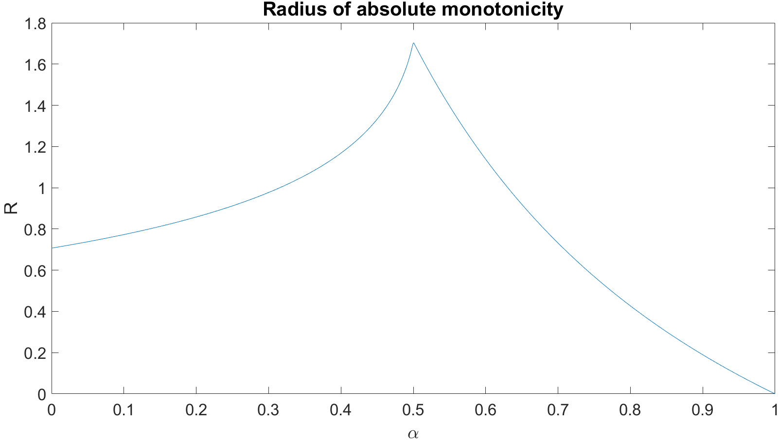
Refer to caption

a) Refer to caption b)

Figure 32: Analysis of the explicit part of IMEX scheme: a) Radius of absolute monotonicity as function of α𝛼\alpha, b) Size of stability region along the imaginary axis as α𝛼\alpha varies.

Appendix B Eigenvalues of 1D Euler equations

In this Appendix we compute the eigenvalues for the Euler equations in non-dimensional form for a general equation of state. For the sake of simplicity, we focus on 1D case and so the equations can be written as follows

ρt+x(ρu)𝜌𝑡𝑥𝜌𝑢\displaystyle\frac{\partial\rho}{\partial t}+\frac{\partial}{\partial x}\left(\rho u\right) =\displaystyle= 00\displaystyle 0
ρut+x(ρu2)+1M2px𝜌𝑢𝑡𝑥𝜌superscript𝑢21superscript𝑀2𝑝𝑥\displaystyle\frac{\partial\rho u}{\partial t}+\frac{\partial}{\partial x}\left(\rho u^{2}\right)+\frac{1}{M^{2}}\frac{\partial p}{\partial x} =\displaystyle= 00\displaystyle 0 (91)
ρEt+x[(ρE+p)u]𝜌𝐸𝑡𝑥delimited-[]𝜌𝐸𝑝𝑢\displaystyle\frac{\partial\rho E}{\partial t}+\frac{\partial}{\partial x}\left[\left(\rho E+p\right)u\right] =\displaystyle= 0.0\displaystyle 0.

This is equivalent to

ρt+uρx+ρux𝜌𝑡𝑢𝜌𝑥𝜌𝑢𝑥\displaystyle\frac{\partial\rho}{\partial t}+u\frac{\partial\rho}{\partial x}+\rho\frac{\partial u}{\partial x} =0absent0\displaystyle=0
ρtu+utρ+u2ρx+2ρuux+1M2px𝜌𝑡𝑢𝑢𝑡𝜌superscript𝑢2𝜌𝑥2𝜌𝑢𝑢𝑥1superscript𝑀2𝑝𝑥\displaystyle\frac{\partial\rho}{\partial t}u+\frac{\partial u}{\partial t}\rho+u^{2}\frac{\partial\rho}{\partial x}+2\rho u\frac{\partial u}{\partial x}+\frac{1}{M^{2}}\frac{\partial p}{\partial x} =0absent0\displaystyle=0 (92)
ρtE+Etρ+(ρE+p)ux+u(ρxE+Exρ+px)𝜌𝑡𝐸𝐸𝑡𝜌𝜌𝐸𝑝𝑢𝑥𝑢𝜌𝑥𝐸𝐸𝑥𝜌𝑝𝑥\displaystyle\frac{\partial\rho}{\partial t}E+\frac{\partial E}{\partial t}\rho+\left(\rho E+p\right)\frac{\partial u}{\partial x}+u\left(\frac{\partial\rho}{\partial x}E+\frac{\partial E}{\partial x}\rho+\frac{\partial p}{\partial x}\right) =0.absent0\displaystyle=0.

Thanks to the continuity equation and to the relation E=e+12M2u2𝐸𝑒12superscript𝑀2superscript𝑢2E=e+\frac{1}{2}M^{2}u^{2}, we obtain

ρt+uρx+ρux𝜌𝑡𝑢𝜌𝑥𝜌𝑢𝑥\displaystyle\frac{\partial\rho}{\partial t}+u\frac{\partial\rho}{\partial x}+\rho\frac{\partial u}{\partial x} =\displaystyle= 00\displaystyle 0
ut+uux+1ρM2px𝑢𝑡𝑢𝑢𝑥1𝜌superscript𝑀2𝑝𝑥\displaystyle\frac{\partial u}{\partial t}+u\frac{\partial u}{\partial x}+\frac{1}{\rho M^{2}}\frac{\partial p}{\partial x} =\displaystyle= 00\displaystyle 0 (93)
et+pρux+uex𝑒𝑡𝑝𝜌𝑢𝑥𝑢𝑒𝑥\displaystyle\frac{\partial e}{\partial t}+\frac{p}{\rho}\frac{\partial u}{\partial x}+u\frac{\partial e}{\partial x} =\displaystyle= 0.0\displaystyle 0.

In general e=e(p,ρ)𝑒𝑒𝑝𝜌e=e(p,\rho), so that

e=eρρ+epp,𝑒𝑒𝜌𝜌𝑒𝑝𝑝\frac{\partial e}{\partial\square}=\frac{\partial e}{\partial\rho}\frac{\partial\rho}{\partial\square}+\frac{\partial e}{\partial p}\frac{\partial p}{\partial\square}, (94)

and, hence, the system reduces to

ρt+uρx+ρux𝜌𝑡𝑢𝜌𝑥𝜌𝑢𝑥\displaystyle\frac{\partial\rho}{\partial t}+u\frac{\partial\rho}{\partial x}+\rho\frac{\partial u}{\partial x} =\displaystyle= 00\displaystyle 0
ut+uux+1ρM2px𝑢𝑡𝑢𝑢𝑥1𝜌superscript𝑀2𝑝𝑥\displaystyle\frac{\partial u}{\partial t}+u\frac{\partial u}{\partial x}+\frac{1}{\rho M^{2}}\frac{\partial p}{\partial x} =\displaystyle= 00\displaystyle 0 (95)
pt+(pρρeρ)epux+upx𝑝𝑡𝑝𝜌𝜌𝑒𝜌𝑒𝑝𝑢𝑥𝑢𝑝𝑥\displaystyle\frac{\partial p}{\partial t}+\frac{\left(\frac{p}{\rho}-\rho\frac{\partial e}{\partial\rho}\right)}{\frac{\partial e}{\partial p}}\frac{\partial u}{\partial x}+u\frac{\partial p}{\partial x} =\displaystyle= 0,0\displaystyle 0,

which can be thought in the following vector form as:

𝐐t+𝐀𝐐x=𝟎𝐐𝑡𝐀𝐐𝑥0\frac{\partial\mathbf{Q}}{\partial t}+\mathbf{A}\frac{\partial\mathbf{Q}}{\partial x}=\mathbf{0} (96)

with

𝐐=[ρup]𝐐matrix𝜌𝑢𝑝\mathbf{Q}=\begin{bmatrix}\rho\\ u\\ p\end{bmatrix} (97)

and

𝐀=[uρ00u1ρM20(pρρeρ)epu].𝐀matrix𝑢𝜌00𝑢1𝜌superscript𝑀20𝑝𝜌𝜌𝑒𝜌𝑒𝑝𝑢\mathbf{A}=\begin{bmatrix}u&\rho&0\\ 0&u&\frac{1}{\rho M^{2}}\\ 0&\frac{\left(\frac{p}{\rho}-\rho\frac{\partial e}{\partial\rho}\right)}{\frac{\partial e}{\partial p}}&u\end{bmatrix}. (98)

The eigenvalues of (98) are u1M1ρpeρρ2ep𝑢1𝑀1𝜌𝑝𝑒𝜌superscript𝜌2𝑒𝑝u-\frac{1}{M}\frac{1}{\rho}\sqrt{\frac{p-\frac{\partial e}{\partial\rho}\rho^{2}}{\frac{\partial e}{\partial p}}}, u𝑢u and u+1M1ρpeρρ2ep𝑢1𝑀1𝜌𝑝𝑒𝜌superscript𝜌2𝑒𝑝u+\frac{1}{M}\frac{1}{\rho}\sqrt{\frac{p-\frac{\partial e}{\partial\rho}\rho^{2}}{\frac{\partial e}{\partial p}}}. The first law of thermodynamics, already recalled in Section 3, provides us the following relation

Tds=depρ2dρ=(eρpρ2)dρ+epdp,𝑇𝑑𝑠𝑑𝑒𝑝superscript𝜌2𝑑𝜌𝑒𝜌𝑝superscript𝜌2𝑑𝜌𝑒𝑝𝑑𝑝Tds=de-\frac{p}{\rho^{2}}d\rho=\left(\frac{\partial e}{\partial\rho}-\frac{p}{\rho^{2}}\right)d\rho+\frac{\partial e}{\partial p}dp, (99)

or, equivalently,

dp=pρ2eρepdρ+Tepds.𝑑𝑝𝑝superscript𝜌2𝑒𝜌𝑒𝑝𝑑𝜌𝑇𝑒𝑝𝑑𝑠dp=\frac{\frac{p}{\rho^{2}}-\frac{\partial e}{\partial\rho}}{\frac{\partial e}{\partial p}}d\rho+\frac{T}{\frac{\partial e}{\partial p}}ds. (100)

Hence, following [53], we have

c2=pρ|s=pρ2eρepc^{2}=\frac{\partial p}{\partial\rho}\bigg{\rvert}_{s}=\frac{\frac{p}{\rho^{2}}-\frac{\partial e}{\partial\rho}}{\frac{\partial e}{\partial p}} (101)

and, therefore, the eigenvalues of (98) are

u+cMuu+cM𝑢𝑐𝑀𝑢𝑢𝑐𝑀u+\frac{c}{M}\ \ \ u\ \ \ u+\frac{c}{M}

also for a generic equation of state, and not only in the case of an ideal gas, as already discussed in [38]. This justifies the definition (75) also in case of non-ideal gases.

References

  • [1] D.N. Arnold. An interior penalty finite element method with discontinuous elements. SIAMNUM, 19:742–760, 1982.
  • [2] W. Bangerth, R. Hartmann, and G. Kanschat. deal II: a general-purpose object-oriented finite element library. ACM Transactions on Mathematical Software (TOMS), 33:24–51, 2007.
  • [3] R.E. Bank, W.M. Coughran, W. Fichtner, E.H. Grosse, Rose D.J., and R.K. Smith. Transient Simulation of Silicon Devices and Circuits. IEEE Transactions on Electron Devices., 32:1992–2007, 1985.
  • [4] F. Bassi, L. Botti, A. Colombo, A. Ghidoni, and F. Massa. Linearly implicit Rosenbrock-type Runge–Kutta schemes applied to the Discontinuous Galerkin solution of compressible and incompressible unsteady flows. Computers & Fluids, 118, 2015.
  • [5] F. Bassi, A. Crivellini, D.A. Di Pietro, and S. Rebay. An implicit high-order discontinuous Galerkin method for steady and unsteady incompressible flows. Computers & Fluids, 36:1529–1546, 2007.
  • [6] L. Bonaventura. A semi-implicit, semi-Lagrangian scheme using the height coordinate for a nonhydrostatic and fully elastic model of atmospheric flows. Journal of Computational Physics, 158:186–213, 2000.
  • [7] L. Bonaventura and A. Della Rocca. Unconditionally strong stability preserving extensions of the TR-BDF2 method. Journal of Scientific Computing, 70:859–895, 2017.
  • [8] L. Bonaventura, R. Redler, and R. Budich. Earth System Modelling 2: Algorithms, Code Infrastructure and Optimisation. Springer Verlag, New York, 2012.
  • [9] S. Boscarino, J. Qiu, G. Russo, and T: Xiong. High Order Semi-implicit WENO Schemes for All-Mach Full Euler System of Gas Dynamics. SIAM Journal on Scientific Computing, 44(2):B368–B394, 2022.
  • [10] W. Boscheri and L. Pareschi. High order pressure-based semi-implicit IMEX schemes for the 3D Navier-Stokes equations at all Mach numbers. Journal of Computational Physics, 434:110206, 2021.
  • [11] S. Busto, M. Tavelli, W. Boscheri, and M. Dumbser. Efficient high order accurate staggered semi-implicit discontinuous Galerkin methods for natural convection problems. Computers & Fluids, 198:104399, 2020.
  • [12] V. Casulli and D. Greenspan. Pressure method for the numerical solution of transient, compressible fluid flows. International Journal for Numerical Methods in Fluids, 4:1001–1012, 1984.
  • [13] M.J.P. Cullen. A test of a semi-implicit integration technique for a fully compressible non-hydrostatic model. Quarterly Journal of the Royal Meteorological Society, 116:1253–1258, 1990.
  • [14] M. Dumbser and V. Casulli. A conservative, weakly nonlinear semi-implicit finite volume scheme for the compressible navier- stokes equations with general equation of state. Applied Mathematics and Computation, 272:479–497, 2016.
  • [15] M. Dumbser, O. Zanotti, R. Loubère, and S. Diot. A posteriori subcell limiting of the discontinuous Galerkin finite element method for hyperbolic conservation laws. Journal of Computational Physics, 278:47–75, 2014.
  • [16] N. Fehn, M. Kronbichler, C. Lehrenfeld, G. Lube, and P. Schroeder. High-order DG solvers for under-resolved turbulent incompressible flows: A comparison of l2superscript𝑙2l^{2} and h(div)𝑑𝑖𝑣h(div) methods. International Journal of Numerical Methods in Fluids, 91:533–556, 2019.
  • [17] M. Fernandez. Propellant tank pressurization modeling for a hybrid rocket. Master’s thesis, Rochester Institute of Technology, 2009.
  • [18] L. Ferracina and M.N. Spijker. Stepsize restrictions for the Total-Variation-Diminishing property in general Runge-Kutta methods. SIAM Journal of Numerical Analysis, 42(3):1073–1093, 2004.
  • [19] M. Gandolfi. Baer-Nunziato type models for the simulation of hybrid rockets self-pressurizing tanks. Master’s thesis, Politecnico di Milano, 2019.
  • [20] U. Ghia, K.N. Ghia, and C.T. Shin. High-Re solutions for incompressible flow using the Navier-Stokes equations and a multigrid method. Journal of Computational Physics, 48(3):387–411, 1982.
  • [21] F.X. Giraldo. Semi-implicit time-integrators for a scalable spectral element atmospheric model. Quarterly Journal of the Royal Meteorological Society, 131:2431–2454, 2005.
  • [22] F.X. Giraldo. An Introduction to Element-Based Galerkin Methods on Tensor-Product Bases. Springer Nature, 2020.
  • [23] F.X. Giraldo, J.F. Kelly, and E.M. Constantinescu. Implicit-explicit formulations of a three-dimensional nonhydrostatic unified model of the atmosphere (NUMA). SIAM Journal of Scientific Computing, 35:1162–1194, 2013.
  • [24] F.X. Giraldo, M. Restelli, and M. Läuter. Semi-implicit formulations of the Navier–Stokes equations: Application to nonhydrostatic atmospheric modeling. SIAM Journal on Scientific Computing, 32:3394–3425, 2010.
  • [25] S. Gottlieb and C.W. Shu. Total variation diminishing Runge-Kutta schemes. Mathematics of Computation, 67(221):73–85, 1998.
  • [26] S. Gottlieb, C.W. Shu, and E. Tadmor. Strong stability-preserving high-order time discretization methods. SIAM Review, 43(1):89–112, 2001.
  • [27] I. Higueras. On strong stability preserving time discretization methods. Journal of Scientific Computing, 21:193–223, 2004.
  • [28] M.E. Hosea and L.F: Shampine. Analysis and implementation of TR-BDF2. Applied Numerical Mathematics, 20:21–37, 1996.
  • [29] B. Janssen and G. Kanschat. Adaptive multilevel methods with local smoothing for H1superscript𝐻1H^{1}- and Hcurlsuperscript𝐻𝑐𝑢𝑟𝑙H^{curl}-conforming high order finite element methods. SIAM Journal on Scientific Computing, 33(4):2095–2114, 2011.
  • [30] G.E. Karniadakis and S. Sherwin. Spectral hplimit-from𝑝hp-Element Methods for Computational Fluid Dynamics. Oxford University Press, 2005.
  • [31] C.A. Kennedy and M.H. Carpenter. Additive Runge-Kutta schemes for convection-diffusion-reaction equations. Applied Numerical Mathematics, 44:139–181, 2003.
  • [32] J.F.B.M. Kraaijevanger. Contractivity of Runge-Kutta methods. BIT, 31:482–528, 1991.
  • [33] C. Kühnlein, W. Deconinck, R. Klein, S. Malardel, Z.P. Piotrowski, P.K. Smolarkiewicz, J. Szmelter, and N.P. Wedi. FVM 1.0: A nonhydrostatic finite-volume dynamical core formulation for IFS. Geoscientific Model Development, 12:651–676, 2019.
  • [34] O. Le Métayer and R. Saurel. The Noble-Abel Stiffened-Gas equation of state. Physics of Fluids, 28:046102, 04 2016.
  • [35] E.W. Lemmon and R. Span. Short fundamental equations of state for 20 industrial fluids. Journal of Chemical & Engineering Data, 51:785–850, 2006.
  • [36] R.J. LeVeque. Finite volume methods for hyperbolic problems. Cambridge University Press, 2002.
  • [37] S.G. Lias, J. Bartmess, J.F. Liebman, J. Holmes, R.D. Levin, and G. Mallard. NIST chemistry webbook standard reference database number 69. National Institute of Standards Technology, 01 2010.
  • [38] C.D. Munz, S. Roller, R. Klein, and K.J. Geratz. The extension of incompressible flow solvers to the weakly compressible regime. Computers and Fluids, 32:173–196, 2003.
  • [39] P. Nederstigt. Real gas thermodynamics: and the isentropic behavior of substances. Master’s thesis, Delft University of Technology, 2017.
  • [40] G. Orlando. A filtering monotonization approach for dg discretizations of hyperbolic problems. Technical Report 2204.08693, arXiv, 2022.
  • [41] G. Orlando, A. Della Rocca, P.F. Barbante, L. Bonaventura, and N. Parolini. An efficient and accurate implicit DG solver for the incompressible Navier‐Stokes equations. to appear in International Journal for Numerical Methods in Fluids, 2022.
  • [42] L. Pareschi and G. Russo. Implicit–explicit Runge–Kutta schemes and applications to hyperbolic systems with relaxation. Journal of Scientific computing, 25:129–155, 2005.
  • [43] M. Restelli. Semi-Lagrangian and Semi-Implicit Discontinuous Galerkin Methods for Atmospheric Modeling Applications. PhD thesis, Politecnico di Milano, 2007.
  • [44] M. Restelli and F.X. Giraldo. A conservative Discontinuous Galerkin semi-implicit formulation for the Navier-Stokes equations in nonhydrostatic mesoscale modeling. SIAM Journal of Scientific Computing, 31:2231–2257, 2009.
  • [45] A. Robert. A semi-Lagrangian and semi-implicit numerical integration scheme for the primitive meteorological equations. Journal of the Meteorological Society of Japan, 60:319–325, 1982.
  • [46] P.K. Smolarkiewicz, C. Kühnlein, and N.P. Wedi. Semi-implicit integrations of perturbation equations for all-scale atmospheric dynamics. Journal of Computational Physics, 376:145–159, 2019.
  • [47] G.A. Sod. A survey of several finite difference methods for systems of nonlinear hyperbolic conservation laws. Journal of Computational Physics, 27(1):1–31, 1978.
  • [48] R. Span. Multiparameter Equations of State. Springer, 2000.
  • [49] J. Steppeler, R. Hess, G. Doms, U. Schättler, and L. Bonaventura. Review of numerical methods for nonhydrostatic weather prediction models. Meteorology and Atmospheric Physics, 82:287–301, 2003.
  • [50] G. Strang. On the construction and comparison of difference schemes. SIAM Journal on Numerical Analysis, 5:506–517, 1968.
  • [51] M. Tavelli and M. Dumbser. A pressure-based semi-implicit space–time discontinuous Galerkin method on staggered unstructured meshes for the solution of the compressible Navier–Stokes equations at all Mach numbers. Journal of Computational Physics, 341:341–376, 2017.
  • [52] G. Tumolo and L. Bonaventura. A semi-implicit, semi-Lagrangian discontinuous Galerkin framework for adaptive numerical weather prediction. Quarterly Journal of the Royal Meteorological Society, 141:2582–2601, 2015.
  • [53] J. Vidal. Thermodynamics: Applications to chemical engineering and petroleum industry. Editions Technip, 2001.
  • [54] J. Zeifang, J. Schütz, K. Kaiser, A. Beck, M. Lukáčová-Medvid’ová, and S. Noelle. A Novel Full-Euler Low Mach Number IMEX Splitting. Communications in Computational Physics, 27(1):292–320, 2019.