Neutrino propagation when mass eigenstates and decay eigenstates mismatch

Abstract

We point out that the Hermitian and anti-Hermitian components of the effective Hamiltonian for decaying neutrinos cannot be simultaneously diagonalized by unitary transformations for all matter densities. We develop a formalism for the two-flavor neutrino propagation through matter of uniform density, for neutrino decay to invisible states. Employing a resummation of the Zassenhaus expansion, we obtain compact analytic expressions for neutrino survival and conversion probabilities, to first and second order in the “mismatch parameter” $\bar{\gamma}$.

Introduction — Neutrino oscillation experiments have unequivocally established that neutrinos have masses, and their flavors mix. However, data still allow the possibility of new physics effects at a sub-leading level. Neutrino decay to lighter invisible states Bahcall:1972my ; Acker:1991ej ; Acker:1993sz is one such possibility. Solutions to neutrino anomalies via a combination of oscillation and decay have been studied Barger:1998xk ; Barger:1999bg ; Choubey:1999ir ; Choubey:2000an ; Bandyopadhyay:2001ct ; Joshipura:2002fb ; Bandyopadhyay:2002qg ; GonzalezGarcia:2008ru ; Berryman:2014qha ; Abrahao:2015rba ; Picoreti:2015ika ; Gomes:2014yua ; Choubey:2018cfz . Most of these papers have analyzed neutrino oscillation probabilities in vacuum, taking the mass eigenstates to be identical with the decay eigenstates for analytical treatment. Matter effects, if relevant, have been implemented numerically.

The effective Hamiltonian for neutrino decay is non-Hermitian, with its Hermitian component corresponding to the energy and the anti-Hermitian component corresponding to decay. The assumption of identifying the mass (energy) eigenstates to decay eigenstates is not valid in general. Indeed, even in vacuum, these two components need not commute, and hence need not be diagonalizable simultaneously by unitary transformations. Even for the special circumstances or models where the mass eigenstates and decay eigenstates coincide in vacuum, matter effects make this mismatch inevitable.

The non-Hermitian Hamiltonian itself may be diagonalized by a similarity transformation employing a non-unitary matrix. Using this principle, the oscillation probabilities in the two-flavor scenario in vacuum were approximately calculated in Berryman:2014yoa . A similar exercise has also been performed in Ascencio-Sosa:2018lbk , albeit in the context of visible neutrino decays in matter, but no compact analytical expressions for probabilities have been presented.

In this Letter, we present a novel prescription for computing the neutrino survival or conversion probabilities for the scenario with simultaneous oscillation and invisible decay of neutrinos propagating in matter of uniform density. We represent the effective Hamiltonian matrix by ${\mathcal{H}}_{m}$, where

$${\mathcal{H}}_{m}=H_{m}-i\Gamma_{m}/2\;.$$ (1)

Here $H_{m}$ and $\Gamma_{m}$ are Hermitian matrices. We choose to work in the basis where the Hermitian part of the Hamiltonian is diagonalized. This is the same as the basis of neutrino mass eigenstates in matter in the absence of decay. In this basis, $H_{m}$ is a diagonal matrix whose elements depend on neutrino mass squared differences, neutrino energy, and Earth matter potential. The flavor evolution of neutrinos takes the form

$${}\nu(t)=e^{-i\mathcal{H}_{m}t}\nu(0)\;.$$ (2)

Note that since $[H_{m},\Gamma_{m}]\neq 0$ in general, $\mathcal{H}_{m}$ is not a normal matrix, and $e^{-i{\mathcal{H}}_{m}t}\neq e^{-iH_{m}t}e^{-\Gamma_{m}t/2}$. Thus, one has to express $e^{-i\mathcal{H}_{m}t}$ in terms of a chain of commutators using the inverse Baker-Campbell-Hausdorff (BCH) formula, also known as the Zassenhaus formula Zassenhaus-Wilhelm ; Zassenhaus-Casas . The standard form of this formula cannot be truncated to a finite number of terms in the current scenario, therefore we employ a resummation technique using its series expansion Kimura:2017xxz . The procedure facilitates a perturbative expansion of the neutrino survival and conversion probabilities, in terms of a small parameter $\bar{\gamma}$ that characterizes the mismatch between the eigenstates of $H_{m}$ and $\Gamma_{m}$.

Our prescription leads to explicit analytical forms for two-flavor neutrino probabilities in matter. The probabilities in vacuum, as well as those calculated by using the assumption of coincident mass and decay eigenstates, emerge as special cases. This formulation is completely new, and provides a clear framework for analyzing neutrino decay in vacuum and matter on the same footing. Moreover, the techniques can be applied to any situation where quantum mechanical evolution in terms of non-Hermitian Hamiltonian is to be calculated.

Formalism — The effective Hamiltonian may be written in the basis of neutrino mass eigenstates in matter as

$$\mathcal{H}_{m}=\left(\begin{array}[]{cc}a_{1}-ib_{1}&-\frac{1}{2}i\gamma e^{i\chi}\\ -\frac{1}{2}i\gamma e^{-i\chi}&a_{2}-ib_{2}\\ \end{array}\right),$$ (3)

where $a_{i},b_{i},\gamma,\chi$ are real. Since $\Gamma_{m}$ needs to be positive semidefinite, $b_{i}\geq 0$ and $\gamma^{2}\leq 4b_{1}b_{2}$. The sign of $\gamma$ is taken to be positive; this defines the value of $\chi$ uniquely. The Hermitian part of this Hamiltonian is diagonal, which is ensured by the choice of basis. The anti-Hermitian part is composed of the diagonal components involving $b_{i}$, and the off-diagonal components involving $\gamma$. Note that $b_{i}=[\Gamma_{m}]_{ii}/2$, and $\gamma e^{i\chi}=[\Gamma_{m}]_{12}=[\Gamma_{m}]_{21}^{*}$.

For future convenience, we define the complex parameter $d_{i}\equiv a_{i}-ib_{i}$, the differences $\Delta_{a}\equiv a_{2}-a_{1},~{}\Delta_{b}\equiv b_{2}-b_{1},~{}\Delta_{d}\equiv d_{2}-d_{1}$, and the dimensionless ratios

$$\bar{\gamma}\equiv\frac{\gamma}{|\Delta_{d}|}\;,\quad\bar{\Delta}_{a}\equiv\frac{\Delta_{a}}{|\Delta_{d}|}\;,\quad\bar{\Delta}_{b}\equiv\frac{\Delta_{b}}{|\Delta_{d}|}\;.$$ (4)

Then, in terms of the identity matrix ${\mathbb{I}}$ and

$$\mathbb{X}\equiv-\frac{i\,\Delta_{d}\,t}{2}\left(\begin{array}[]{cc}-1&0\\ 0&1\end{array}\right)\;,\mathbb{Y}\equiv-\frac{\gamma t}{2}\left(\begin{array}[]{cc}0&e^{i\chi}\\ e^{-i\chi}&0\end{array}\right)\;,$$ (5)

one may write

$$-i\mathcal{H}_{m}t=-\frac{it}{2}\,(d_{1}+d_{2})\,\mathbb{I}+\mathbb{X}+\mathbb{Y}\;.$$ (6)

The commutator of $\mathbb{X}$ and $\mathbb{Y}$ is

$${\mathcal{L}}_{\mathbb{X}}\mathbb{Y}\equiv[\mathbb{X},\mathbb{Y}]=i\frac{\gamma\,\Delta_{d}\,t^{2}}{2}\left(\begin{array}[]{cc}0&-e^{i\chi}\\ e^{-i\chi}&0\end{array}\right)\;,$$ (7)

which will play a key role in our analysis.

Zassenhaus expansion — In order to calculate the evolution matrix $e^{-i{\mathcal{H}}_{m}t}$, keeping aside the term proportional to the identity matrix, we need to calculate the quantity $e^{\mathbb{X}+\mathbb{Y}}$. This may be written in terms of the Zassenhaus expansion Zassenhaus-Wilhelm ; Zassenhaus-Casas as

$${}e^{\mathbb{X}+\mathbb{Y}}=e^{\mathbb{X}}\,e^{\mathbb{Y}}\,e^{-\frac{1}{2}[\mathbb{X},\mathbb{Y}]}\,e^{\frac{1}{6}(2[\mathbb{Y},[\mathbb{X},\mathbb{Y}]]+[\mathbb{X},[\mathbb{X},\mathbb{Y}]])}...$$ (8)

Note that $|\mathbb{Y}|\sim\bar{\gamma}|\mathbb{X}|$ and ${\mathcal{L}}_{\mathbb{X}}\mathbb{Y}\sim\bar{\gamma}|\mathbb{X}|^{2}$, where the absolute sign $(|\cdot|)$ represents a typical nonzero element in the corresponding matrix. This implies that, in general, for higher-order commutators, ${\mathcal{L}}^{k-1}_{\mathbb{X}}\mathbb{Y}\sim\bar{\gamma}|\mathbb{X}|^{k}$. Therefore, it is not possible to truncate the expansion in eq. (8) at any fixed order of commutators. One needs to collect $O(\gamma^{k})$ terms from commutators of all orders by performing a resummation procedure. We therefore employ the expression for the Zassenhaus expansion in terms of a series Kimura:2017xxz :

$${}e^{\mathbb{X}+\mathbb{Y}}=\Big{(}1+\Big{.}\Big{.}\sum\limits_{p=1}^{\infty}\sum\limits_{n_{1},...,n_{p}=1}^{\infty}\dfrac{n_{p}...n_{1}}{n_{p}(n_{p}+n_{p-1})...(n_{p}+...+n_{1})}\mathcal{Y}_{n_{p}}...\mathcal{Y}_{n_{1}}\Big{)}e^{\mathbb{X}}\;,$$ (9)

where $\mathcal{Y}_{n}=\frac{1}{n!}\mathcal{L}^{n-1}_{\mathbb{X}}\mathbb{Y}$.

To obtain the expansion up to $O(\bar{\gamma})$ and $O(\bar{\gamma}^{2})$, we need to perform the summation for $p=1$ and $p=1,2$, respectively, since every ${\mathbb{Y}}$ comes with a factor of $\bar{\gamma}$. Thus for an accuracy of $O(\bar{\gamma}^{2})$, we can truncate

$${}e^{\mathbb{X}+\mathbb{Y}}\approx\Big{(}1+\sum\limits_{n_{1}=1}^{\infty}\mathcal{Y}_{n_{1}}+\sum\limits_{n_{1}=1}^{\infty}\sum\limits_{n_{2}=1}^{\infty}\dfrac{n_{1}}{(n_{1}+n_{2})}\mathcal{Y}_{n_{2}}\mathcal{Y}_{n_{1}}\Big{)}e^{\mathbb{X}},$$ (10)

with the double summation term not needed for $O(\bar{\gamma})$ accuracy. One may use

$$\mathcal{Y}_{n}=\frac{1}{n!}(i\Delta_{d}t)^{n-1}\sigma_{3}^{n-1}\mathbb{Y}\;$$ (11)

in order to get closed functional forms for the infinite sums. Here $\sigma_{3}$ is the Pauli matrix.

Neutrino flavor conversions up to $O(\bar{\gamma})$ — The truncation of the right hand side of eq. (10) to the first summation gives

$${}e^{\mathbb{X}+\mathbb{Y}}=\left(1+\dfrac{\sin(\Delta_{d}t)}{\Delta_{d}t}\mathbb{Y}-\dfrac{\cos(\Delta_{d}t)-1}{\Delta_{d}t}i\sigma_{3}\mathbb{Y}\right)e^{\mathbb{X}}.$$ (12)

The amplitude matrix in the mass basis in matter is then

$${}\mathcal{A}_{m}\equiv e^{-i\mathcal{H}_{m}t} = \left(\begin{array}[]{cc}e^{-id_{1}t}&-i\frac{\gamma e^{i\chi}g_{-}(t)}{\Delta_{d}}\\ -i\frac{\gamma e^{-i\chi}g_{-}(t)}{\Delta_{d}}&e^{-id_{2}t}\\ \end{array}\right),$$ (15)

where the functions $g_{\pm}(t)$ are defined as

$$g_{\pm}(t)=\frac{1}{2}(e^{-id_{2}t}\pm e^{-id_{1}t})\;.$$ (16)

The neutrino flavor conversion probability $P_{\beta\alpha}$ for $\nu_{\beta}\to\nu_{\alpha}$ conversion may be obtained by calculating the flavor conversion amplitude

$$[\mathcal{A}_{f}]_{\alpha\beta}=\left[U_{m}\;e^{-i\mathcal{H}_{m}t}\;U_{m}^{\dagger}\right]_{\alpha\beta}\;,$$ (17)

and further, $P_{\beta\alpha}=|{\cal A}_{\alpha\beta}|^{2}$. In the 2-flavour system,

$$U_{m}=\left(\begin{array}[]{cc}\cos\theta_{m}&\sin\theta_{m}\\ -\sin\theta_{m}&\cos\theta_{m}\\ \end{array}\right)$$ (18)

is the unitary rotation matrix. One can write

$${}\mathcal{A}_{f}=\left(\begin{array}[]{cc}g_{-}(t)A(\chi)+g_{+}(t)&g_{-}(t)B(\chi)\\ g_{-}(t)B(-\chi)&-g_{-}(t)A(\chi)+g_{+}(t)\\ \end{array}\right)\;,$$ (19)

where $A(\chi)$ and $B(\chi)$ are given in Table 1. The $\chi$-dependence of $A$ and $B$ is implicit wherever not stated explicitly.

Table 1: The terms in the amplitude matrix ${\mathcal{A}}_{f}$ in the flavor basis used in eq. (19), calculated up to $O(\bar{\gamma})$.

Term	Expression
$A(\chi)\equiv A^{(0)}+\gamma A^{(1)}$	$\begin{aligned} \smash[b]{\vphantom{\bigg{|}}}-\cos 2\theta_{m}-i\dfrac{\gamma}{\Delta_{d}}\sin 2\theta_{m}\cos\chi\smash[t]{\vphantom{\bigg{|}}}\end{aligned}$
$B(\chi)\equiv B^{(0)}+\gamma B^{(1)}$	$\begin{aligned} \smash[b]{\vphantom{\bigg{|}}}\sin 2\theta_{m}-i\dfrac{\gamma}{\Delta_{d}}\Big{(}\cos 2\theta_{m}\cos\chi+i\sin\chi\Big{)}\smash[t]{\vphantom{\bigg{|}}}\end{aligned}$

The survival probability of a neutrino of flavor $\alpha$ is

$${}\begin{split}P_{\alpha\alpha}=&\frac{e^{-(b_{1}+b_{2})t}}{2}\Big{[}(1+|A|^{2})\cosh(\Delta_{b}t)\Big{.}\\ &+(1-|A|^{2})\cos(\Delta_{a}t)-2\text{Re}(A)\sinh(\Delta_{b}t)\\ &\Big{.}+2\text{Im}(A)\sin(\Delta_{a}t)\Big{]}\;.\end{split}$$ (20)

The survival probability $P_{\beta\beta}$ for the other flavor may be obtained from $P_{\alpha\alpha}$ with the replacement $A\to-A$. The probability for $\nu_{\beta}\to\nu_{\alpha}$ conversion is

$${}P_{\beta\alpha}=\frac{e^{-(b_{1}+b_{2})t}}{2}|B(\chi)|^{2}\,[\cosh(\Delta_{b}t)-\cos(\Delta_{a}t)]\;.$$ (21)

The conversion probability $P_{\alpha\beta}$ is obtained by the replacement $\chi\to-\chi$. The explicit expressions for the terms in eqs. (20) and (21) are given in Table 2.

Table 2: The terms to be used in the probabilities shown in eqn.(20) and (21), calculated up to $O(\bar{\gamma})$.

Term	Expression
$\text{Re}(A)$	$\begin{aligned} \smash[b]{\vphantom{\bigg{|}}}-\cos 2\theta_{m}+\bar{\gamma}\bar{\Delta}_{b}\sin 2\theta_{m}\cos\chi\smash[t]{\vphantom{\bigg{|}}}\end{aligned}$
$\text{Im}(A)$	$\begin{aligned} \smash[b]{\vphantom{\bigg{|}}}-\bar{\gamma}\bar{\Delta}_{a}\sin 2\theta_{m}\cos\chi\smash[t]{\vphantom{\bigg{|}}}\end{aligned}$
$|A|^{2}$	$\begin{aligned} \smash[b]{\vphantom{\bigg{|}}}\cos^{2}2\theta_{m}-2\bar{\gamma}\bar{\Delta}_{b}\sin 2\theta_{m}\cos 2\theta_{m}\cos\chi\smash[t]{\vphantom{\bigg{|}}}\end{aligned}$
$|B|^{2}$	$\begin{aligned} \smash[b]{\vphantom{\bigg{|}}}\sin^{2}2\theta_{m}+2\bar{\gamma}\sin 2\theta_{m}\Big{(}\bar{\Delta}_{a}\sin\chi+\bar{\Delta}_{b}\cos 2\theta_{m}\cos\chi\Big{)}\smash[t]{\vphantom{\bigg{|}}}\end{aligned}$

It should be noted that in the two-flavor approximation in the absence of neutrino decay, i.e. $b_{1}=b_{2}=\gamma=0$, we have $P_{\alpha\alpha}=P_{\beta\beta}$ and $P_{\beta\alpha}=P_{\alpha\beta}$. These equalities no longer hold in the presence of decay.

Neutrino flavor conversions up to $O(\bar{\gamma}^{2})$ — For probabilities accurate up to order $\bar{\gamma}^{2}$, we need to calculate the term in eq.(10) that involves a double summation. This sum may be rewritten as

$$\dfrac{1}{2}\sum\limits_{n_{1}=1}^{\infty}\left(\sum\limits_{n_{2}=1}^{\infty}\mathcal{Y}_{n_{2}}\mathcal{Y}_{n_{1}}+\sum\limits_{n_{2}=n_{1}}^{\infty}\frac{n_{1}-n_{2}}{n_{1}+n_{2}}[\mathcal{Y}_{n_{2}},\mathcal{Y}_{n_{1}}]\right),$$ (22)

whose closed form may be obtained using the observation

$$[\mathcal{Y}_{n_{2}},\mathcal{Y}_{n_{1}}]=\frac{(-1)^{n_{2}}-(-1)^{n_{1}}}{4n_{1}!n_{2}!}(i\Delta_{d}t)^{n_{2}+n_{1}-2}(\gamma t)^{2}\sigma_{3}\;.$$ (23)

The eigenvalues of ${\mathcal{H}}_{m}$ get corrections at $O(\bar{\gamma}^{2})$, and it is convenient to write the probabilities at this (and higher) order in terms of the difference of the exact eigenvalues

$$\Delta_{D}=\sqrt{\Delta_{d}^{2}-\gamma^{2}}\;.$$ (24)

The probabilities at $O(\bar{\gamma}^{2})$ can be written in the same form as eqs. (20) and (21) with the replacements

$$\Delta_{a}\to{\rm Re}(\Delta_{D})\;,\quad\Delta_{b}\to-{\rm Im}(\Delta_{D})\;,$$ (25)

and the entries in Table 1 replaced by

$$A(\chi) \to A^{(0)}+\gamma A^{(1)}-\gamma^{2}\cos 2\theta_{m}/(2\Delta_{d}^{2})\;,$$ (26)

$$B(\chi) \to A^{(0)}+\gamma A^{(1)}+\gamma^{2}\sin 2\theta_{m}/(2\Delta_{d}^{2})\;,$$ (27)

The entries corresponding to Table 2 can be calculated using eqs. (26) and (27).

Exact results — For the 2-flavor system, it is also possible to obtain the exact expressions for neutrino survival and conversion probabilities by expressing $-i{\mathcal{H}}_{m}t$ as a linear combination of Pauli matrices nielsen2002quantum . For any $2\times 2$ matrix $\mathbb{K}$, one can write

$$e^{\mathbb{K}}=e^{k_{0}}\left[\mathbb{I}~{}\cosh k+\frac{\vec{k}\cdot\vec{\sigma}}{k}~{}\sinh k\right],$$ (28)

where $k_{\mu}\equiv{\rm Tr}(\mathbb{K}\cdot\sigma_{\mu})/2$, and $k\equiv\sqrt{k_{1}^{2}+k_{2}^{2}+k_{3}^{2}}$. For the matrix $\mathbb{K}=-i{\mathcal{H}}_{m}t$ as in eq. (3), this corresponds to

$$k_{0}=-\frac{it}{2}(d_{1}+d_{2})\;,\;k=\frac{it\Delta_{D}}{2}\;.$$ (29)

This leads to the exact probabilities that can be written in the same form as eqs. (20) and (21), with the replacements given in eq. (25), and

$$A(\chi)\to\frac{\Delta_{d}}{\Delta_{D}}A(\chi)\quad \quad B(\chi)\to\frac{\Delta_{d}}{\Delta_{D}}B(\chi)\;,$$ , (30)

in Table 1.

The entries corresponding to Table 2 can be calculated using eq. (30).

Numerical comparison — We now demonstrate, using numerical calculations, the convergence of our analytical results towards the exact neutrino oscillation probabilities, when higher and higher order terms in $\bar{\gamma}$ are included. For the sake of illustration, we choose the survival probability of $\nu_{\mu}$ with energy $E\sim$ GeV, for a baseline of 295 km. This would correspond to the probability relevant at the T2K/T2HK experiment.

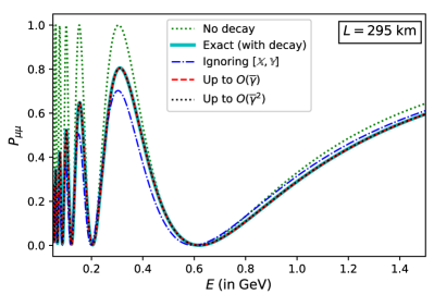
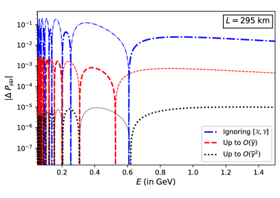
Figure 1: The left panel shows the survival probability $P_{\mu\mu}$ calculated exactly, and by using the analytical expressions in the text, in the presence and absence of neutrino decay. The right panel shows the differences between the analytical expressions and the exact results for decay. The thick (thin) lines correspond to $\Delta P_{\mu\mu}>0$ ($\Delta P_{\mu\mu}<0$). The sharp dips in the right panel correspond to those energies where the analytical expressions give the same values as the exact ones.

We take the parameters of the Hermitian part of the Hamiltonian to be $\Delta_{a}=2.56\times 10^{-3}\text{ eV}^{2}/(2E),\theta_{m}=45^{\circ}$, and the parameters of the anti-Hermitian part to be $(b_{1},b_{2},\gamma)=(3,6,8)\times 10^{-5}\mbox{ eV}^{2}/(2E),\chi=\pi/4$. Note that the parameters $a_{i},b_{i},\gamma$ from Eq. (3) are taken to vary as $1/E$ to account for time dilation.

The left panel in Fig. 1 shows the probability $P_{\mu\mu}(E)$ without decay, and successive approximations at $O(\bar{\gamma})$ and $O(\bar{\gamma}^{2})$ in the presence of decay. The incorrect approximation that neglects the commutator $[\mathbb{X},\mathbb{Y}]$ is also indicated. The convergence towards the exact solution is more clearly demonstrated in the right panel of Fig. 1, where we show the values of the error

$$|\Delta P_{\mu\mu}|\equiv P_{\mu\mu}\mbox{(analytical)}-P_{\mu\mu}\mbox{(exact)}\;$$ (31)

on a logarithmic scale. Clearly, the inclusion of $O(\bar{\gamma})$ and $O(\bar{\gamma}^{2})$ terms reduces the error by orders of magnitude.

Comparison with earlier results — In ref. Berryman:2014yoa , neutrino decay in vacuum was analyzed using diagonalization of the non-Hermitian Hamiltonian with ${\mathcal{H}}_{\rm diag}=N^{-1}{\mathcal{H}}N$, using a non-unitary matrix $N$. We find that the most general form of the non-unitary matrix that would diagonalize a non-Hermitian ${\mathcal{H}}$ is

$$N=\left(\begin{array}[]{cc}\cos\theta_{m}&\sin\theta_{m}\\ -\sin\theta_{m}&\cos\theta_{m}\\ \end{array}\right)\left(\begin{array}[]{cc}1&-i\frac{\gamma e^{i\chi}}{\Delta_{D}+\Delta_{d}}\\ i\frac{\gamma e^{-i\chi}}{\Delta_{D}+\Delta_{d}}&1\\ \end{array}\right)\;.$$ (32)

Note that since $(\Delta_{D}+\Delta_{d})$ is complex, the off-diagonal elements of the second matrix in eq. (32) are not complex conjugates of one another, an assumption implicitly made in ref. Berryman:2014yoa . This introduces corrections in the neutrino conversion probabilities of $\sim O(\bar{\gamma}\bar{\Delta}_{b})$. These may be neglected if one assumes $\bar{\Delta}_{b}\sim O(\bar{\gamma})$; however, these will then contribute to $O(\bar{\gamma}^{2})$ corrections.

For the special case with only one unstable neutrino, whose decay eigenstate in vacuum coincides with one of the mass eigenstates $\nu_{2}$ in vacuum, the probabilities in matter may be obtained by the following identifications:

$$a_{1,2}=\frac{\tilde{m}_{1,2}^{2}}{2E}\quad \quad b_{1,2}=\frac{\alpha_{2}}{4E}[1\mp\cos[2(\theta-\theta_{m})]\;,$$ , (33)

$$\chi=0\quad \quad\gamma=\frac{\alpha_{2}}{2E}\sin[2(\theta-\theta_{m})].$$ , (34)

Here, $\tilde{m}_{i}(m_{i})$ and $\theta_{m}(\theta)$ are the mass eigenvalues and mixing angle in matter (vacuum), and $\alpha_{2}=m_{2}/\tau_{2}$, where $\tau_{2}$ is the lifetime of $\nu_{2}$ in vacuum. Note that both mass eigenstates in matter now undergo decay, and the off-diagonal term $\gamma$ is generated, even though it was absent in vacuum. This prescription gives the correct analytical probability expressions for decaying neutrinos in matter, which are hitherto not explicitly given in the literature. In the limit $\theta_{m}\to\theta$ and $\tilde{m}_{i}\to m_{i}$, the standard probabilities for decay in vacuum Lindner:2001fx are obtained.

Concluding remarks — Neutrino decay is characterized by a non-Hermitian Hamiltionian, which cannot be diagonalized with a unitary transformation. Further, there is no guarantee that decay eigenstates are the same as the mass eigenstates, although it is usually assumed. We point out that even if these two sets are the same in vacuum, matter effects necessarily change this simple picture, warranting a more careful treatment.

In this Letter, we develop a novel formalism which can address the above two issues, and allows one to obtain compact analytical forms for two flavour probabilities even in matter. The crucial step in our formulation is to perform the analysis in the basis of mass eigenstates in matter in the absence of decay, so that the Hermitian component of the Hamiltonian is diagonal. The anti-Hermitian decay matrix is not diagonal in this basis, and does not commute with the Hermitian part. This prompts us to employ the Zassenhaus (inverse BCH) expansion for the time evolution matrix. Further, we introduce a resummation of commutators to compute the neutrino survival and conversion probabilities perturbatively in $\bar{\gamma}$, the parameter characterizing the mismatch between mass and decay eigenstates. This is the first time such a formulation has been used to treat propagation of unstable neutrinos in matter.

While the explicit results in this work are calculated in the context of a two-flavor scenario, the framework of perturbative expansion in $\bar{\gamma}$ may be easily extended to three flavors. Moreover, the scope of application of this method goes beyond just the neutrino decay hypothesis; the formalism may be applied to various other phenomena such as the combined treatment of oscillations and absorption for high energy neutrinos, axion-photon oscillations in an optically semi-opaque medium, or even the neutral meson mixing systems.

Acknowledgments — D.S.C. would like to thank S. Moitra for useful discussions. S.G. and L.S.M. would like to thank S. Choubey and C. Gupta for useful discussions. A.D. acknowledges support from the Department of Atomic Energy (DAE), Government of India, under Project Identification No. RTI4002. S.G. acknowledges the J.C Bose Fellowship (JCB/2020/000011) of Science and Engineering Research Board of Department of Science and Technology, Government of India.

References

- (1) J. N. Bahcall, N. Cabibbo, and A. Yahil, “Are neutrinos stable particles?,” Phys. Rev. Lett. 28 (1972) 316–318.
- (2) A. Acker, S. Pakvasa, and J. T. Pantaleone, “Decaying Dirac neutrinos,” Phys. Rev. D 45 (1992) 1–4.
- (3) A. Acker and S. Pakvasa, “Solar neutrino decay,” Phys. Lett. B 320 (1994) 320–322, arXiv:hep-ph/9310207.
- (4) V. D. Barger, J. Learned, S. Pakvasa, and T. J. Weiler, “Neutrino decay as an explanation of atmospheric neutrino observations,” Phys. Rev. Lett. 82 (1999) 2640–2643, arXiv:astro-ph/9810121.
- (5) V. D. Barger, J. Learned, P. Lipari, M. Lusignoli, S. Pakvasa, and T. J. Weiler, “Neutrino decay and atmospheric neutrinos,” Phys. Lett. B 462 (1999) 109–114, arXiv:hep-ph/9907421.
- (6) S. Choubey and S. Goswami, “Is neutrino decay really ruled out as a solution to the atmospheric neutrino problem from Super-Kamiokande data?,” Astropart. Phys. 14 (2000) 67–78, arXiv:hep-ph/9904257.
- (7) S. Choubey, S. Goswami, and D. Majumdar, “Status of the neutrino decay solution to the solar neutrino problem,” Phys. Lett. B 484 (2000) 73–78, arXiv:hep-ph/0004193.
- (8) A. Bandyopadhyay, S. Choubey, and S. Goswami, “MSW mediated neutrino decay and the solar neutrino problem,” Phys. Rev. D 63 (2001) 113019, arXiv:hep-ph/0101273.
- (9) A. S. Joshipura, E. Masso, and S. Mohanty, “Constraints on decay plus oscillation solutions of the solar neutrino problem,” Phys. Rev. D 66 (2002) 113008, arXiv:hep-ph/0203181.
- (10) A. Bandyopadhyay, S. Choubey, and S. Goswami, “Neutrino decay confronts the SNO data,” Phys. Lett. B 555 (2003) 33–42, arXiv:hep-ph/0204173.
- (11) M. Gonzalez-Garcia and M. Maltoni, “Status of Oscillation plus Decay of Atmospheric and Long-Baseline Neutrinos,” Phys. Lett. B 663 (2008) 405–409, arXiv:0802.3699 [hep-ph].
- (12) J. M. Berryman, A. de Gouvea, and D. Hernandez, “Solar Neutrinos and the Decaying Neutrino Hypothesis,” Phys. Rev. D 92 no. 7, (2015) 073003, arXiv:1411.0308 [hep-ph].
- (13) T. Abrahão, H. Minakata, H. Nunokawa, and A. A. Quiroga, “Constraint on Neutrino Decay with Medium-Baseline Reactor Neutrino Oscillation Experiments,” JHEP 11 (2015) 001, arXiv:1506.02314 [hep-ph].
- (14) R. Picoreti, M. Guzzo, P. de Holanda, and O. Peres, “Neutrino Decay and Solar Neutrino Seasonal Effect,” Phys. Lett. B 761 (2016) 70–73, arXiv:1506.08158 [hep-ph].
- (15) R. Gomes, A. Gomes, and O. Peres, “Constraints on neutrino decay lifetime using long-baseline charged and neutral current data,” Phys. Lett. B 740 (2015) 345–352, arXiv:1407.5640 [hep-ph].
- (16) S. Choubey, D. Dutta, and D. Pramanik, “Invisible neutrino decay in the light of NOvA and T2K data,” JHEP 08 (2018) 141, arXiv:1805.01848 [hep-ph].
- (17) J. M. Berryman, A. de Gouvêa, D. Hernández, and R. L. N. Oliveira, “Non-Unitary Neutrino Propagation From Neutrino Decay,” Phys. Lett. B 742 (2015) 74–79, arXiv:1407.6631 [hep-ph].
- (18) M. V. Ascencio-Sosa, A. M. Calatayud-Cadenillas, A. M. Gago, and J. Jones-Pérez, “Matter effects in neutrino visible decay at future long-baseline experiments,” Eur. Phys. J. C 78 no. 10, (2018) 809, arXiv:1805.03279 [hep-ph].
- (19) W. Magnus, “On the exponential solution of differential equations for a linear operator,” Communications on Pure and Applied Mathematics 7 no. 4, (1954) 649–673.
- (20) F. Casas, A. Murua, and M. Nadinic, “Efficient computation of the zassenhaus formula,” Computer Physics Communications 183 no. 11, (Nov, 2012) 2386–2391, arXiv:1204.0389 [math-ph].
- (21) T. Kimura, “Explicit Description of the Zassenhaus Formula,” PTEP 2017 no. 4, (2017) 041A03, arXiv:1702.04681 [math-ph].
- (22) M. A. Nielsen and I. Chuang, “Quantum computation and quantum information,” American Association of Physics Teachers (2002).
- (23) M. Lindner, T. Ohlsson, and W. Winter, “A Combined treatment of neutrino decay and neutrino oscillations,” Nucl. Phys. B 607 (2001) 326–354, arXiv:hep-ph/0103170.