An optimization model for renewal scheduling and traffic flow routing

Abstract

This document is the third sub-report from the research project SATT (Samplanering av trafikpåverkande åtgärder och trafikflöden, modellstudie / Coordinated planning of temporary capacity restrictions and traffic flows, model study). The report summarizes the modelling alternatives that have been considered. The main result of the model study is that we propose a bi-level approach for handling the two parts of the problem, i.e. the scheduling of renewal projects and the subsequent adjustments of railway traffic flow. The contributions are: (1) a mixed integer formulation for scheduling project tasks, and (2) a network flow formulation for establishing the possible volumes of railway traffic during the imposed capacity restrictions of these project tasks. The intended usage of the model is for economical planning of a specific production year, which takes place before the timetabling process starts. This document introduces the problem and gives a full description of (1) along with results from computational experiments that have been conducted with this model. An accompanying report gives the details of the final formulation of (2).

1 Introduction

An infrastructure manager is responsible for the capacity planning of a transportation network. The long term planning consists of deciding on renewal, upgrade, and major maintenance activities which constitute large budget volumes for a national railway system. Thus, a multi-annual economical planning is necessary. This planning is done before the details of the railway traffic (aka the timetable) are known. Nevertheless, there is a need to understand the implications that the project planning has on the train traffic that will take place alongside the project tasks. Hence, the long-term economical planning should both ensure that the considered infrastructure projects can be completed, while at the same time limiting the negative impact of these projects on the on-going traffic. This planning problem is sometimes labeled as “intervention planning” [3].

In this work we study the coordination of major capacity affecting work activities and traffic flows, by developing a method for optimal scheduling of project tasks, which considers both the project aspects and the traffic throughput. We are particularly interested in major work tasks that take place on an existing railway network, such as upgrades, renewals and larger maintenance activities. Thus we disregard investment projects and the construction of new infrastructure which does not interact with any on-going train traffic. Also, we do not consider activities with minor capacity impact, such as shorter and recurrent regular maintenance, which are, or can be, handled in the tactical and operational planning.

1.1 Background, motivation and problem description

The current planning of railway renewal projects in Sweden is done with a limited view of the traffic impact. Each project is treated individually and network wide effects, particularly the combinatorial effects of several or all projects, are not supported by the available planning methods or tools. In fact, very few examples of such planning support can be found in the research literature. Instead, rough assumptions are made regarding traffic volumes, and the capacity impact is estimated based on experience and with advisory tables regarding which work types and work locations that might or should not be conducted at the same time. There are few performance indicators and metrics for measuring the traffic impact, limited knowledge about the actual capacity effects of previously conducted projects, and no strong decision support for dimensioning, configuring and scheduling renewal projects.

On the other hand, there is a growing awareness for the need of well founded quantitative planning methods. Especially when governmental spending is increasing as a consequence of aging infrastructure, historical asset management deficits, and an increase in railway transportation demand. In this situation, the coordination of capacity needs from renewal and traffic activities must be balanced with the intention of achieving an optimal outcome for society (according to available resources).

The need for improved decision support regarding the scheduling of renewal projects in the long-term economical (intervention) planning is the motivation for this study. The purpose of the work is to investigate the possibility of using mathematical optimization techniques for this planning stage.

The requirement details for the planning problem has been elaborated in [5]. The resulting problem definition can be stated as follows: Given a railway network with an assumed transportation flow demand and a set of considered renewal projects, each consisting of a sequence of work tasks with specific resource needs (e.g. machines and crew), schedule as many projects as possible with a minimal combined cost for task resource usage and traffic disruptions, such that limitations regarding project timing, resource availability, capacity restrictions, and traffic flow, is respected. The intention is to be able to solve problem instances for national networks and a scheduling period of one operational year.

1.2 Literature overview

Scheduling methods for railways have traditionally focused on train traffic. Some examples of well studied problems are timetabling, rolling stock and crew scheduling, rostering, routing, rescheduling, speed optimization, etc. In recent years the coordination and joint scheduling of maintenance and traffic have attracted some research activity, but so far mostly regarding tactical planning where each train service is individually scheduled. Such optimization model have been able to solve weekly problem instances [6]. Although the basic problem type (coordination of work tasks and train traffic) is similar, these models are too fine-grained regarding the traffic representation to suit the requirements for yearly renewal scheduling. However, the aggregated network representation and capacity control applied for example by [7] is an approach that is suitable in our problem setting.

As for aggregated handling of national railway traffic flows, there are limited references in the optimization literature. However, in [1] a model for describing railway transportation in the form of so called “transport service classes” is presented. The idea is to describe a (future) national transportation plan with these transport service classes, based on origin-destination relations, travel time and crucial service requirements, while giving the freedom of fulfilling these transport service classes with different routing options. When traffic is described in this form, there is no need to consider individual trains or train paths. Instead the traffic can be represented as flows, where appropriate link capacity constraints should ensure that a feasible timetable exists for this flow. This kind of traffic representation is suitable for our problem setting.

The above given references was the starting inspiration for this work. In [5] a survey of other related research is presented. The literature search focused on publications that treat both track works and train traffic in a long-term setting, where the latter is represented on an aggregated level—not as timetables and individual trains but as flows of traffic. The publications were categorized according to the temporal resolution regarding work and traffic flow. Models where the activity type are shorter than the time period lengths, such that they always can start and complete within one time period, we label as “static”. If the activities span over more than one time period, such that the partial overlapping of activities becomes crucial, we use the term “dynamic” (see for example Skutella (2009) regarding timed, or dynamic, network flows). Thus, we get four types of models, namely:

• Coarse models, where both work activities and traffic flow is static. A common example is to consider which year to perform different projects, but where the project time is considerably shorter and where traffic impact is treated without consideration of synchronization or network effects.

• Work-flexible models with static traffic, where track work activities span over several time periods but the traffic flows have no interaction between time periods. A typical time resolution for such models would be to use a weekly or daily period length.

• Traffic-flexible models with static work activities, where traffic flows will interact between time periods while each work activity only affect one time period. Thus there is no partial overlap between work activities and the capacity restrictions imposed on the traffic is fixed within each time period.

• Work- and traffic-flexible models, where both track work activities and traffic flows span over more than one time period, such that the dynamic effects over the network topology must be considered.

We aim at the last type of model, but the bulk of research literature has only been found in the two first types (with static traffic flow modeling). From the coarse models we have not found any applicable modeling inspiration apart from [4] which use different time scales for track works and link status. This is an idea that could be applied to our case for upgrade projects and traffic flow.

The work-flexible models with static traffic show a large variation regarding level of details and which aspects that are considered for the track works. However, all these models have the limitation that each track work only consists of one uninterrupted activity (or task). These references however indicate that a combination of a mixed integer programming and a network flow formulation (for track works and traffic respectively) might be suitable in our problem setting.

Finally we have not been able to find any traffic-flexible models based on traffic flows with properties that fit railway systems and the planning problem we consider. This indicates either that our search has been too limited or that we have found a research gap where important and interesting contributions can be made.

1.3 Outline of work and document overview

The modeling work started by considering an approach based on a set partitioning formulation with two types of columns, one for project schedules and one for traffic flow routing. A model sketch of this is given in Appendix A, first for an integrated model, then for a bi-level approach. At this stage focus was given to the traffic model (the lower level of the bi-level approach) and instead of column generation we worked on network flow formulations. Three variants (with different layer definitions) were studied. An overview of these alternatives is given in Section 2.2 and the details of the first two can be found in Appendix B. The third formulation of the traffic flow model is documented in the accompanying report [2]. The last stage of the modeling work concerned the scheduling of upgrade projects (the upper level of the bi-level approach), where a mixed integer formulation was developed. The mathematical model is presented in Section 2.3 followed by results from computational experiments in Chapter 3. The document ends with some final conclusions and discussion in Chapter 4.

2 Mathematical formulation

We propose a bi-level approach where the two parts of the problem are treated in two interconnected models, as illustrated in Figure 1. The upper level is the scheduling of the upgrade projects according to an initial cost function. For each operational day which is affected by (temporary) capacity restrictions (TCRs), the subsequent traffic adjustments are calculated by the lower level problem. Thus, only the affected traffic days need to be considered in the lower level, which reduces the problem size. The obtained traffic adjustments can then be considered by the upper level problem in order to find a better TCR schedule, taking both the cost for the upgrade projects and the traffic routing into account. The two processes are iterated until some convergence or optimality criteria is met.

Figure 1: Bi-level model outline

In the remainder of this chapter we describe the modeling in more detail. Section 2.1 gives some basic notation, followed by an outline of the flow-based formulation models that have been investigated for the lower level problem (Section 2.2). Finally, the complete formulation of the upper level model is given in Section 2.3.

2.1 Basic notation

The following basic notation will be used throughout the document.

Planning period

$T$	a sequence of time periods $t$
$\beta_{t},\delta_{t}$	start and length of time period $t\in T$

As a simplification we will mostly assume a unit time period length ($\delta_{t}=1$) where each time period $t$ starts at $\beta_{t}=t-1$, and spans the open-ended time interval $[t-1,t)$.

Railway network

$N$	a set of network nodes $n$
$L$	a set of network links $l$
$C_{l}^{nom}$	the nominal capacity (number of trains per time unit) for link $l\in L$

Wanted traffic

$H$	a set of train types $h$
$R$	a set of traffic relations $r$, each defined by an origin-destination-train type tuple $(o_{r},d_{r},h_{r})\in N\times N\times H$

For each traffic relation there is a limited set of routing options through the network, which we will discuss in subsequent sections.

Renewals / upgrade projects

$U$	a set of upgrade projects $u$, which in turn consists of a sequence of tasks.

The details regarding project tasks will be further described in Section 2.3.

2.2 Flow based approach of the lower level problem

The idea of the flow based formulation is to describe the problem as a layered space-time network problem, where time is discretized into relatively coarse time periods, say of length 1–6 hours, such that the link travel time for all trains are shorter than any time period length. If we let $\nu$ be the travel time expressed as a share of the time period length, this means that we require $0<\nu<1$. Assuming that flow is evenly distributed over the time period, then $1-\nu$ of the flow will arrive within the same time period and $\nu$ of the flow in the next time period. We further demand flow continuity such that no incoming flow from the previous time period ($t-1$) into time period $t$ is allowed to proceed to the succeeding time period ($t+1$). With this requirement we avoid situations where flow might “jump hurdles”, and in addition the formulation complexity is reduced. For a situation of two connected links $p$ and $l$, with (relative) travel times $\nu_{p}$ and $\nu_{l}$, the requirement is then $\nu_{p}+\nu_{l}\leq 1$ (or $1-\nu_{p}-\nu_{l}\geq 0$). A simple and conservative limitation is to require $\nu\leq\frac{1}{2}$, but a more flexible approach is to surround (long) links where $\nu\geq 0.5$ with shorter ones, such that the requirement holds.

These concepts are illustrated in Figure 2 for two successive links ($p$ and $l$), where bold arrows indicate flow variables, named as follows:

$x_{lt}^{Tr,d}$	Transportation flow over link $l$, starting in time period $t$ and arriving in the same time period (direct flow)
$x_{lt}^{Tr,f}$	Transportation flow over link $l$, starting in time period $t$ and arriving in the next period $t+1$ (forward flow)
$x_{nt}^{Ni}$	Node inventory flow for node $n$ between time period $t$ and $t+1$

Figure 2: Illustration of flow relations.

The consequence of the continuity requirement is that $x_{lt}^{Tr,f}\leq x_{pt}^{Tr,d}$, and that we can impose constraints that control the volumes of direct and forward flow, so as to achieve proper travel times through the network.

The next important question concerns the layer definition. We have investigated three approaches:

• One layer per train type $h$

• One layer per origin-destination relation $r$

• One layer per routing option $p$ of each traffic relation $r$, where each routing option constitutes one path through the network

The two first options are described in more detail in Appendix B along with some computational experiments. Both models allow for flow to split and merge within each layer. The first model does not properly handle reachability requirements for the traffic relations, while the second (which is a multi-commodity network flow model with side constraints) resolves this issue. However, both models have a major drawback when flow runs over many links, which results in small fractional flow volumes being pushed forward in time (due to the side constraints that control the volumes of direct and forward flow). We have not found any good solution to this problem, and have therefore developed the third model, with one layer for each relation+routing option. This approach gives a planar graph for each layer, and enables another way of imposing travel time restrictions by giving $\nu_{rpn}$ values that state the shortest (relative) travel time (from the origin) for reaching node $n$ of path $p$ and relation $r$, which in turn will restrict the maximum flow volumes that can reach a node at each time period $t$. This model correctly pushes traffic forward in time without the drawbacks of the first two models, although the number of layers, variables and constraints will increase.

The full description of the “routing-option flow model” is given in the accompanying report [2].

2.3 MIP formulation of the upper level problem

This section contains a model write-up of the upper level problem as a MIP formulation. First, we introduce some additional input data:

$T_{u}\subseteq T$	The allowed set of time periods (from start to end) for upgrade project $u$
$W_{u}$	The number of work tasks in upgrade project $u$
$\eta_{uw}$	The length (number of time periods) for work task $w$ of upgrade project $u$
$\gamma_{uw},\theta_{uw}$	The min and max length (number of time periods) of rest time between work task $w$ and $w+1$ of upgrade project $u$
$b_{uwl}$	The number of capacity blockings caused by work task $w$ of upgrade project $u$ on link $l$
$F_{d}(\mathbf{x}^{d})$	Disruption cost for traffic assignment $\mathbf{x}^{d}$ of day $d$
$K$	The set of all work resources $k$
$g_{uwk}$	The amount of resource usage for work resource $k$ when performing work task $w$ of project $u$
$Q_{k}$	The available quantity of work resource $k$

The basic decision variables in the model are

$y_{uwt}\in\mathbb{Z}_{2}^{U\times W\times T}$	(Binary) Whether work task $w$ of upgrade project $u$ is taking place during time period $t$ or not
$z_{uwt}\in\mathbb{Z}_{2}^{U\times W\times T}$	(Binary) Whether work task $w$ of upgrade project $u$ is starting in time period $t$ or not
$s_{u}\in\mathbb{Z}_{2}^{U}$	(Binary) Whether upgrade project $u$ is canceled (not scheduled) or not
$q_{k}\in\mathbb{R}_{+}^{K}$	The max usage of resource $k$ in any time period

We assume that each work task has a fixed duration (can easily be changed) and that the tasks within an upgrade project should be performed in their given order. The decision freedom lies in selecting start times of each work task, while respecting the spacing requirements between successive tasks. The optimization problem can then be formulated as follows:

$$\textrm{minimize}\sum_{u\in U}c_{u}^{U}s_{u}+\sum_{k\in K}c_{k}^{K}q_{k}+\sum_{d\in WD\left(\bar{\mathbf{y}}\right)}F_{d}\left(\mathbf{x}^{d}\right)\\ +\sum_{l\in L.t\in T}\lambda_{lt}\left(a_{lt}\left(\mathbf{x}\right)+\sum_{u\in U}\sum_{w=1}^{W_{u}}b_{uwl}y_{uwt}-C_{l}^{nom}\right)$$

subject to constraints for:

scheduling each work task once unless project is canceled

$$\forall u\in U,w\in\left[1,W_{u}\right]: \sum_{t\in T_{u}}z_{uwt}=1-s_{u};$$ (1)

linking on-going work variables to work start variables

$$\forall u\in U,w\in\left[1,W_{u}\right],t\in T_{u}: z_{uwt}\geq y_{uwt}-y_{uw,t-1};$$ (2)

length of each work task

$$\forall u\in U,w\in\left[1,W_{u}\right],t\in T_{u}: \sum_{i=1}^{\min(\eta_{uw},t)}z_{uw,t-i+1}=y_{uwt};$$ (3)

no overlapping tasks within a project

$$\forall u\in U,t\in T_{u}: \sum_{w=1}^{W_{u}}y_{uwt}\leq 1;$$ (4)

successive order of tasks within a project

$$\forall u\in U,w\in\left[1,W_{u}-1\right],i\in\left[1,W_{u}-w\right],t\in T: \sum_{j=1}^{t}\left(z_{uwj}-z_{u,w+i,j}\right)\geq 0;$$ (5)

minimum and maximum length of rest time between tasks

$$\forall u\in U,w\in\left[1,W_{u}-1\right],t\in T_{u}: \sum_{i=1}^{\min(\gamma_{uw},\left|T\right|-t)}z_{u,w+1,t+i}\leq\sum_{j=1}^{t}z_{uwj}-y_{uwt};$$ (6)

$$\forall u\in U,w\in\left[1,W_{u}-1\right],t\in T_{u}: \sum_{i=1}^{\min(\theta_{uw},\left|T\right|-t)}z_{u,w+1,t+i}\geq\sum_{j=1}^{t}\left(z_{uwj}-z_{u,w+1,j}\right)-y_{uwt};$$ (7)

and limited resource usage

$$\forall k\in K,t\in T: \sum_{u\in U}\sum_{w=1}^{W_{u}}g_{uwk}y_{uwt}\leq q_{k};$$ (8)

$$\forall k\in K: q_{k}\leq Q_{k}.$$ (9)

Note that the objective function penalizes unscheduled work tasks, resource usage, traffic disruption cost and a Lagrangian relaxation term for line capacity utilization. Work costs could be added, and coordination of certain activities (e.g. interlocking or traffic management system loading) can be achieved by setting time period limitations on work task level (i.e. using data sets $T_{uw}$ rather than $T_{u}$).

This formulation uses a large number of variables and constraints. As an example, consider a one year planning period divided into 6 hour periods, which results in $365\times 4=1460$ time periods. Then the scheduling of 100 upgrade projects, each consisting of (in average) 10 work tasks, where each project has an allowed scheduling period of 4 months ($\Rightarrow 4\times 30\times 4=480$ time periods) will require in the order of 1 M variables and 2.5 M constraints. However, if time period limitations are set on work task level, such that each work task has on average a one month scheduling window, the problem size is reduced to about 250 k variables and 750 k constraints. Such problem sizes can be tractable for modern LP and MIP solvers. An alternative could be to use a CP approach, especially for handling resource limitations and for further pruning of the variable domains (while still handling the optimization problem in a LP/MIP solver). It could also be considered to use real/integer valued task start variables (rather than the binary $z_{uwt}$) so as to reduce the number of variables and get a more compact formulation.

The objective function relies on knowledge of the traffic disruption cost ($F_{d}$) and the traffic capacity usage ($a_{lt}$) over each link and time period, as calculated by the lower level traffic assignment problem. Without knowledge of the actual traffic assignment (for a particular project plan), it is necessary to have some estimate of the traffic impact for a certain project schedule. We can use the blocking values $b_{uwl}$ to setup a proxy for the traffic impact. As a lower bound we can use the largest blocking value for any link during each time period—assuming perfect coordination such that all other blocking values during the same time period does not further affect the traffic. As an upper bound we instead sum all blocking values used at all links and time periods, which corresponds to having no traffic coordination at all. To establish these values we introduce the variables

$x_{t}^{b,m}\in\mathbb{R}_{+}^{T}$	The largest blocking value for any project on any link in time period $t$
$B^{LB},B^{UB}\in\mathbb{R}_{+}$	The lower and upper bound values for number of blocked (affected) trains

and the constraints

$$\forall u\in U,l\in L,t\in T: \sum_{w=1}^{W_{u}}b_{uwl}y_{uwt}\leq x_{t}^{b,m}$$ (10)

$$B^{LB}=\sum_{t\in T}x_{t}^{b,m}$$ (11)

$$B^{UB}=\sum_{u\in U}\sum_{w=1}^{W_{u}}\sum_{l\in L}\sum_{t\in T}b_{uwl}y_{uwt}$$ (12)

Note that $x_{t}^{b,m}$ will become the largest blocking value of any upgrade project $u$ that affect the same link in the same time period. Thus it is assumed that project tasks on the same link are possible to coordinate. (A more conservative approach would be to sum up overlapping blocking values from different projects in the left hand side of the first constraint.) This model can be further improved by including a link-time-dependent cost factor, such that blockings can be made more or less costly depending on the normal traffic load over specific links and time periods. Thus, the values $x_{t}^{b,m}$ and $B^{LB/UB}$ will measure the estimated traffic disruption rather than unavailable train slots.

The values $B^{LB}$ and $B^{UB}$ can be used in the objective function, for example by using a parameter value, $0\leq\zeta\leq 1$ that estimate the level of possible traffic coordination, and adding a cost component

$$c^{disr}\left[\zeta B^{LB}+\left(1-\zeta\right)B^{UB}\right]$$

Additionally, we might want to track time periods with disturbed traffic, using a variable $x_{t}^{d}\in\mathbb{Z}_{2}^{T}$ and the following constraints

$$\forall u\in U,w\in\left[1,W_{u}\right],t\in T: y_{uwt}\leq x_{t}^{d}$$

$$\forall t\in T: x_{t}^{d}\leq\sum_{u\in U}\sum_{w=1}^{W_{u}}y_{uwt}$$

with the possibility to include $x_{t}^{d}$ in the objective function.

For the separation of work tasks it is possible to include an additional set of variables

$e_{uw}\in\mathbb{R}_{+}^{U\times W}$

Start time for work task $w$ of upgrade project $u$

and the following constraints

$$\forall u\in U,w\in\left[1,W_{u}\right]: e_{uw}=\sum_{t\in T}tz_{uwt}$$ (13)

$$\forall u\in U,w\in\left[1,W_{u}-1\right]: e_{u,w+1}-e_{uw}\geq\left(1-s_{u}\right)\left(\eta_{uw}+\gamma_{uw}\right)$$ (14)

$$\forall u\in U,w\in\left[1,W_{u}-1\right]: e_{u,w+1}-e_{uw}\leq\left(1-s_{u}\right)\left(\eta_{uw}+\theta_{uw}\right)$$ (15)

Computational experiments on a limited set of instances indicate that these variables and constraints improve solving performance in most cases. Furthermore these constraints make it possible to disable one or both of the previously given constraints (6) and (7) for minimum and maximum length of rest time between tasks. Our experiments indicate a slight performance gain for removing the minimum rest time constraints (6).

3 Computational experiments

The MIP formulation for the upper level problem (upgrade project scheduling) has been implemented in MiniZinc (version 2.5.5) and solved with COIN-BC (version 2.10.5) as optimization solver. The experiments have been run on a HP EliteBook 830 G5 with an 1.6 GHz i5 processor, 8 GB RAM, and 64 bit Windows 10 Enterprise OS (version 19043.867). We include the event time variables $e_{uw}$ and the corresponding task separation constraints (13)–(15), but exclude the minimum rest time constraints (6) and (7). A small data instance have been used, with 8 nodes and 9 links (see Figure 7). Three projects with 3, 7 and 5 work tasks respectively are to be scheduled and the task lengths, min/max rest time, resource usage and link blocking values are given in Table 1. Directly from the input data we can deduce that the projects must span 14–28, 34–58 and 28–55 time periods respectively, that the minimum resource usage is 1 and 10 (for resources R1 and R2), and that the minimum link blocking for each project is 20, 38 and 52 respectively.

Proj/	Task	Rest time	Usage		Link blocking
Task	len.	Min/Max	R1	R2	A-C	B-C	C-E	C-F	E-H	F-H	D-E	E-F	F-G
P1/W1	2	2/6	0	4			2		2
P1/W2	4	4/8	1	8	1		3		3
P1/W3	2	-/-	0	4			2		2
P2/W1	2	2/6	0	4	2
P2/W2	2	2/6	0	4		2
P2/W3	2	2/6	0	6	1	1	1	1
P2/W4	4	4/8	1	10	2		3
P2/W5	4	4/8	1	10		2		3
P2/W6	2	2/6	0	6	1	1	1	1
P2/W7	2	-/-	0	6	1	1	1	1
P3/W1	1	2/7	0	4							2		2
P3/W2	2	2/8	0	8							1	2	1
P3/W3	8	8/20	1	8							5	5	5
P3/W4	2	2/6	0	8							1	2	1
P3/W5	1	-/-	0	4							2		2

Table 1: Project schedule settings for small test case

In the experiments we will use unit resource costs ($c_{k}^{K}=1,\forall k)$, the traffic disruption cost factor $c^{disr}=0.1$ and a traffic coordination parameter value $\zeta=0.75$. The solving performance will depend on the scheduling freedom for each project, but we will not impose any restrictions on the time windows for each project. Thus there is a large number of symmetric solutions.

Three sets of experiments will be reported. In Section 3.1 and Section 3.2 we will focus solely on the traffic disruption cost and the resource usage respectively. From these experiments we obtain lower bounds which are then used in Section 3.3 to analyse the combined cost of both traffic disruption and resource cost.

3.1 Traffic disruption cost

In this experiment we find lower bounds for the traffic disruption cost by forcing all projects to be scheduled ($s_{u}=0,\forall u$), disregarding the resource costs ($c_{k}^{K}=0,\forall k$), and solving the scheduling problem for four planning period sizes ($\left|T\right|=35,40,45,50$). The results are given in Table 2, which reports the resulting problem sizes (number of variables x constraints), time for finding the integer solution (seconds), total solution time (seconds), the lower bound blocking value ($B^{LB}$), the disruption cost, and the resource usage (R1+R2) for the respective schedule solutions. The latter values are given in parentheses to indicate that they are not considered in the objective function and hence not reliable.

$\left|T\right|$	ProbSize	IPTime	SolTime	$B^{LB}$	DisrCost	ResUse
35	2.0k x 4.4k	1.1	1.3	67	11.525	(2+22)
40	2.3k x 5.0k	24	27	66	11.450	(2+26)
45	2.6k x 5.6k	113	163	66	11.450	(2+26)
50	2.9k x 6.3k	23	742	66	11.450	(2+26)

Table 2: Traffic disruption lower bound for different planning freedoms

First we can establish that the lowest possible $B^{LB}=66$ for this instance. Secondly we see a linear growth in problem size, but a much larger growth in total solution time (although the integer solution is found fairly quickly). This shows the difficulty in proving optimality when having large scheduling freedom and many symmetric solutions. Finally we note that a low blocking value comes at the price of a high resource usage.

The obtained solutions for $\left|T\right|=35$ and $\left|T\right|=40$ are shown as a Gantt view in Figure 3. As expected, we see that the project tasks are coordinated so as to reduce the traffic disruption cost. The two solutions have the same structure – the only principal difference is that the two last tasks of P3 are placed differently. The latter solution has a lower blocking value, but cannot be achieved for $\left|T\right|=35$ (due to the minimum rest time requirement of 8 time periods after P3/W3 in combination with the task lengths and min rest times for the final tasks of the projects). This example shows the interplay of schedule length, task settings, blocking values and cost factors. Finally, we note that the initial task groups are spaced differently in the two solutions, which does not affect the objective value. Hence the task spacing is arbitrary, unless restricted by other factors. Time-dependent blocking costs, e.g. letting time periods with little traffic have lower blocking cost, would remedy this arbitrariness (and reduce the symmetries of the problem).

Figure 3: Schedule solutions with minimal traffic disruption.

We now investigate the effect of supplying the valid lower bound $B^{LB}\geq 66$ to the MIP solver. Table 3 shows the improvement in solving performance. We see that the time for proving optimality is reduced substantially, while there is less improvement in the time for finding integer solutions.

$\left|T\right|$	Without lb	With lb	Relative change
35	1.1 : 1.3	0.7 : 0.8	- 36 : 38 %
40	24 : 27	26 : 26	+8 : -4 %
45	113 : 163	79 : 79	- 30 : 51 %
50	23 : 742	28 : 28	+22 : -96 %

Table 3: Solving performance (IPTime : SolTime) without and with lower bound on blocking value $B^{LB}$

3.2 Resource usage

In the next experiment we disregard the traffic disruptions by setting $c^{disr}=0$, and instead only focus on the resource usage (with unit resource costs $c_{k}^{K}=1,\forall k$). Again we solve for the four planning period sizes and obtain the results as shown in Table 4 (with the same columns as in Table 2). A Gantt view of the first three solutions are shown in Fig 4. We see that the tasks become separated from each other, which reduces the resource usage (while increasing the traffic blocking values). A slight increase in solution time can be noted with increasing planning period size, but there is no tail effect for proving optimality (SolTime is very close to IPTime). Thus the solver has no difficulty in establishing a lower bound for the resource usage (despite the existence of solution symmetries) as opposed to what was observed for the traffic disruption cost in Table 2.

$\left|T\right|$	ProbSize	IPTime	SolTime	$B^{LB}$	DisrCost	ResUse
35	2.0k x 4.4k	0.4	0.4	(130)	(16.250)	2+18
40	2.3k x 5.0k	18.6	18.8	(180)	(20.000)	1+12
45	2.6k x 5.6k	22.1	22.1	(185)	(20.375)	1+10
50	2.9k x 6.3k	34.6	34.6	(185)	(20.375)	1+10

Table 4: Resource usage lower bound for different planning freedoms

Figure 4: Schedule solutions with minimal resource usage.

We now check the effect of introducing a simple valid lower bound, $q_{k}\geq\left(1-s_{u}\right)\max_{w}(g_{uwk})\>\forall u,k$, on the resource usage. The improvement in solution times is listed in Table 5. Once again we see an improvement in solution times—this time both for finding integer solutions and for proving optimality. We also note that there is no increase in solution time with increasing planning period size (for this problem instance).

$\left|T\right|$	Without lb	With lb	Relative change
35	0.4 : 0.4	0.6 : 0.6	+25 : 25 %
40	18.6 : 18.8	9.8 : 9.8	- 47 : 48 %
45	22.1 : 22.1	10.7 : 10.7	- 52 : 52 %
50	34.6 : 34.6	8.5 : 8.5	- 75 : 75 %

Table 5: Solving performance (IPTime : SolTime) without and with lower bound on resource usage

3.3 Combined traffic disruption and resource usage cost

The final experiment concerns the problem of optimizing the sum of traffic disruption and resource usage cost. We perform this test with all combinations of supplying valid lower bounds for blocking value and resource usage. The obtained solutions are presented in Table 6 and the performance comparison for the valid lower bounds are presented in Table 7 and 8, where the first table shows the result of supplying the general lower bounds ($B^{LB}\geq 66$, $q_{R1}\geq 1$, and $q_{R2}\geq 10$) while the second table gives the performance when supplying specific lower bounds for the particular planning problem size (as obtained from Tables 2 and 4). Columns two to five list the solving performance (IPTime : SolTime) in seconds without supplied lower bounds (No lb), with valid bounds on blocking value (B lb), resource usage (Res lb) and both blocking value and resource usage (B+Res lb). For reference we also show the Gantt view of the first three solutions in Figure 5.

The solutions use the minimal amount of resources while the traffic disruption cost goes up, which is in accordance with the chosen cost factors. Hence the work tasks are primarily separated from each other (so as to reduce resource usage), and only grouped together (for reduced traffic disruption) as long as it does not increase the resource usage. The primary performance gain comes from the valid lower bound on resource usage, while the lower bound on the blocking value has less effect. Supplying both lower bounds reduces the time for proving optimality but sometimes hampers the time for finding the best integer solution. Specific lower bound values further improve the solving performance, but might not be justified when considering the additional effort of establishing these specific values.

$\left|T\right|$	$B^{LB}$	DisrCost	ResUse
35	69	11.675	2+18
40	95	13.625	1+12
45	101	14.075	1+10
50	101	14.075	1+10

Table 6: Results for combined traffic disruption and resource usage cost

$\left|T\right|$	No lb	B lb	Res lb	B+Res lb
35	5.3 : 5.3	3.3 : 3.4	4.6 : 4.6	4.4 : 4.5
40	30 : 38	39 : 42	41 : 45	27 : 29
45	333 : 393	197 : 240	124 : 221	61 : 206
50	161 : 1764	110 : 1773	304 : 1305	418 : 1300

Table 7: Performance without and with general lower bound values

$\left|T\right|$	No lb	B lb	Res lb	B+Res lb
35	5.3 : 5.3	4.1 : 4.1	3.8 : 3.9	0.6 : 2.8
40	30 : 38	(39 : 42)	32 : 32	12 : 14
45	333 : 393	(197 : 240)	160 : 212	33 : 149
50	161 : 1764	(110 : 1773)	293 : 1302	325 : 1130

Table 8: Performance without and with specific lower bound values

Figure 5: Schedule solutions with optimal traffic disruption plus resource usage cost

From these computational experiments we first conclude that symmetry reduction, shorter planning horizons, and smaller scheduling freedom for the work tasks are the primary factors for achieving shorter solution times. Supplying valid lower bounds can also improve the solving performance substantially. In particular it helps to give a lower bound for the aspect that dominates the objective value—in this case the resource usage.

4 Conclusions and discussion

The bi-level approach which have been described in this report fits the requirements of renewal project scheduling and traffic flow routing. In particular, it decomposes the problem into its two major aspects and enables the use of different mathematical formulations and time resolutions in the two problem levels. Thus, two important combinatorial problems can be tackled, one for solving the coordination of work tasks for several upgrade projects, and the other for optimally adjusting the network traffic due to imposed capacity restrictions. By iterating between these two problems, the combined planning problem as described in Section 1.1 can be addressed.

So far, we have only been able to conduct computational experiments on the two models separately and the integration into one bi-level model remains to be done. However, the network flow model has so far shown good performance and at this moment we are positive about the tractability of this formulation. Furthermore, this flow approach for handling network wide railway traffic on a macroscopic scale is useful in its own right, particularly when analyzing transportation plans, traffic flows and network capacity without the need for any timetable data.

The mixed integer model for project scheduling has so far only been evaluated on small problem instances. There are some concerns regarding the scalability of this approach, and it might be necessary to use some heuristic or matheuristic approach when treating larger planning problems. However, the handling of traffic blockings and the lower/upper bound estimation of traffic impact from concurrent capacity restrictions enables the upper level to consider the potential traffic disruptions before invoking the detailed lower level computations. It might also be possible to calibrate, perhaps in an adaptable approach, the level of possible traffic coordination (parameter $\zeta$) for different network, traffic and project relations.

Finally, we have so far not treated the multi-annual planning problem. In that setting, some additional features need to be introduced—primarily budget limitations between years (when allowing projects to be moved between years), and possibly (discounted) values of increasing quality costs when renewals are delayed vs service improvements after project completion. In any case, the bi-level approach described in this document, is a promising starting point for the multi-annual planning case.

Appendices

Appendix A Sketch of set partitioning / column generation model

The scheduling of upgrade projects and traffic flow could be formulated as a set partitioning / column generation model. Here we roughly sketch this, by first considering an integrated approach with two types of columns: one for the traffic assignment and one for upgrade project scheduling. Given the major difference in time resolution for these two aspects we then sketch a bi-level approach, where the upper level schedules the upgrade projects, while the lower level treats the subsequent adjustment of the traffic.

A common notation is used as follows. For each traffic relation there is a limited number of routing options, but an enormous amount of timed flow assignments that schedule the trains along these routing options:

$\mathbb{P}_{r}$	all (considered) timed flow assignments $p$ for traffic relation $r$.
$\mathbf{a}_{rp}$	a column vector for flow assignment $p\in\mathbb{P}_{r}$ (of traffic relation $r$), where the column values $a_{rp}^{lt}$ are the number of trains that utilize link $l$ in time period $t$.
$x_{rp}$	binary variable corresponding to each $\mathbf{a}_{rp}$.
$c_{rp}^{T}$	the attributed cost value for flow assignment $p\in\mathbb{P}_{r}$.

For each upgrade project $u\in U$ there are also an enormous amount of possible work schedules:

$\mathbb{V}_{u}$	all (considered) work schedules for upgrade project $u$.
$\mathbf{b}_{uv}$	a column vector for work schedule $v\in\mathbb{V}_{u}$ (of upgrade $u$), where the column values $b_{uv}^{lt}$ are the number of capacity blockings caused on link $l$ in time period $t$.
$y_{uv}$	binary variable corresponding to $\mathbf{b}_{uv}$.
$c_{uv}^{W}$	the attributed cost value for work schedule $v\in\mathbb{V}_{u}$ for upgrade $u$.

A.1 Integrated approach for joint project and traffic scheduling

In an integrated approach the master problem contains both column types, and two sub-problems will be used for generating new cost reducing columns. The master problem is to find flow assignments for all traffic relations and work schedules for all upgrade projects that minimizes the objective

$$\sum_{r\in R,p\in\mathbb{P}_{r}}c_{rp}^{T}x_{rp}+\sum_{u\in U,v\in\mathbb{V}_{u}}c_{uv}^{W}y_{uv}$$

subject to the restrictions that:

Exactly one routing configuration $p$ should be allocated to each service $r$

$$\forall r\in R:\,\sum_{p\in\mathbb{P}_{r}}x_{rp}=1;$$

Exactly one schedule $v$ for each upgrade $u$ should be chosen

$$\forall u\in U:\,\sum_{v\in\mathbb{V}_{u}}y_{uv}=1;$$

And for each link $l$ and time period $t$, the sum of allocated trains and the number of capacity blockings must not exceed the nominal link capacity

$$\forall l\in L,t\in T:\,\sum_{r\in R,p\in\mathbb{\mathbb{P}}_{r}}a_{rp}^{lt}x_{rp}+\sum_{u\in U,v\in\mathbb{V}_{u}}b_{uv}^{lt}y_{uv}\leq C_{l}^{nom}.$$

The sub-problem pricing procedures will then use the dual values from these constraints to generate potential cost reducing columns. However, as noted above, the time horizon as well as the time resolution of these columns differ substantially.

A.2 Bi-level approach

The basis for the bi-level approach is to split the two parts of the problem into two different solving processes. The upper level is the scheduling of the upgrade projects according to an initial cost function. For each operational day which is affected by one or more (temporary) capacity restriction (TCR), the subsequent traffic adjustments are calculated by the lower level problem. Thus, only the affected traffic days needs to be considered in the lower level, which reduces the problem size. The obtained traffic adjustments can then be considered by the upper level problem in order to find a better TCR schedule, taking both the cost for the project schedule and the traffic flow into account. The two processes are iterated until some convergence or optimality criteria is met.

This approach opens up for using different objective functions in the two levels, as well as using different modeling and solution approaches. Furthermore, we can use different discretisations of time on the upper and lower level, which suits the two different types of schedules. For upgrades, the schedules are on macro level, i.e. weeks and days, possibly down to hours. For transports, the schedules are on a finer detail, from hours down to minutes.

We now introduce some further notation, so as to be able to consider resource usage in the upper level, and to only consider disturbed days in the lower level, as follows:

$WD(\mathbf{y})$	set of disrupted (working) days for upgrade project schedule $\mathbf{y}$
$F_{d}(\mathbf{x}^{d})$	disruption cost for traffic assignment $\mathbf{x}^{d}$ of day $d$
$K$	the set of all resources
$Q_{k}$	number of available resources $k$
$L_{k}^{K}$	set of links that resource $k$ can service
$T_{k}^{K}$	set of time periods that resource $k$ can service
$q_{k}$	(variable) max resource usage of resource $k$ in any work period $t$
$g_{uv}^{ktl}$	usage of resource $k$ during time instance $t$ on link $l$, for upgrade $u$ and schedule $v$

A.2.1 The upper level

The upper level problem schedules the upgrade projects. The objective is to minimize the sum of work costs, resource usage, and traffic penalties based on the adjusted traffic from the lower level.

$$\text{Min}\sum_{u\in U,v\in V}c_{uv}^{W}y_{uv}+\sum_{k\in K}c_{k}^{K}q_{k}+\sum_{d\in WD(\mathbf{y})}F_{d}(\mathbf{x}^{d})$$

subject to restrictions that:

Exactly one schedule $v$ should be chosen for each upgrade $u$

$$\forall u\in U:\sum_{v\in\mathbb{V}_{u}}y_{uv}=1$$

Consumed capacity on link $l$ for time period $t$ must be respected (where $C_{lt}$ is the estimated traffic capacity need)

$$\forall t\in T,l\in L:\,\sum_{u\in U,v\in V_{u}}b_{uv}^{lt}y_{uv}\leq C_{l}^{nom}-C_{lt}$$

Usage of resource $k$ in any time period cannot exceed $Q_{k}$

$$\forall k\in K,t\in T_{k}^{K}:\,\sum_{l\in L_{k}^{K}}g_{uv}^{ktl}\sum_{u\in U,v\in v_{k}}y_{uv}\leq q_{k}\leq Q_{k}$$

Note that the values $C_{lt}$ constitute the capacity connection between the upper and lower level problems.

A.2.2 The lower level

The lower level problem schedules the trains, with the capacity restrictions from the upper level as input. The objective is to find an optimal traffic schedule. Note that this is not necessarily the schedule that through-puts as much trains as possible, other factors may also affect what is an optimal schedule such as conformity over the year, regularity, robustness as well as steadiness.

We will first concentrate on the individual trains and a cyclic period, where the objective is to find assignments of transport tasks, defined by origin-destination pairs with periodic repetition.

$$\text{Min}\sum_{r\in R,p\in Pr}c_{rp}^{T}x_{rp}$$

subject to restrictions that:

Exactly one flow assignment (routing and timing) $p$ is chosen for each transport $r$

$$\forall r\in R:\sum_{p\in P_{r}}x_{rp}=1$$

Consumed capacity by traffic must respect the capacity restrictions $C_{lt}$ on each link $l$ and time period $t$, which is the remaining capacity according to the current upgrade project schedule $\mathbf{y}$

$$\forall t\in T,l\in L:\,\sum_{r\in R,p\in P_{r}}a_{rp}^{lt}x_{rp}\leq C_{lt}$$

By letting the traffic schedules be either calculated as cyclic with repetition or by solving instances of consecutive time frames, longer periods can be calculated in the lower level model. In both cases, it will be possible to calculate the cost $F_{d}(\mathbf{x}^{d})$ for each working day $d$.

Appendix B Flow based traffic assignment idea

The following is a write-up of two flow based formulations which were done in parallel with implementation and testing. The first attempt is a model that only distinguishes between train types. After that we describe a multi-commodity model, which correctly will handle the reachability requirements of all origin-destination relations, but allows for flow splitting and merging in the nodes. The two final subsections discuss the problem sizes of these two formulations and reports on the initial computational experiments.

B.1 Aggregating over train types

The basic notation for planning period, railway network and wanted traffic is the same as described in Section 2.1. The traffic assignment problem can be represented by a directed graph $\mathcal{G}\left(\mathcal{V},\mathcal{A}\right)$ with a vertex set $\mathcal{V}\coloneqq\left\{v_{nth}|n,t,h\in N\times T\times H\right\}$ and an arc set $\mathcal{A}\coloneqq\mathcal{A}^{Tr}\cup\mathcal{A}^{Ni}$ which is the union of link transportation arcs $\mathcal{A}^{Tr}$ and node inventory arcs $\mathcal{A}^{Ni}$.

Each vertex $v_{nth}\in\mathcal{V}$ collects the number of trains of type $h$ that start, pass or end in node $n$ during time period $t$. Let $n(i)$, $t(i)$, and $h(i)$ mean the node, the time period and train type of vertex $i$ respectively. Then the link transportation arcs $a_{ij}\in\mathcal{A}^{Tr}$ describe all possible train traffic from vertex $i$ to vertex $j$ such that $\left(n(i),n(j)\right)\in L$, $t(i)\leq t(j)\leq t(i)+1$, and $h(i)=h(j)$. Similarly, the node inventory arcs $a_{ij}\in\mathcal{A}^{Ni}$ describe possible train dwelling at stations between vertex $i$ and $j$ such that $n(i)=n(j)$, $t(i)+1=t(j)$, and $h(i)=h(j)$. Thus the graph will be partitioned according to the train types and transportation can only move forward in time, but must also arrive no later than in the next time period. Furthermore we impose the restriction that the travel time for any train type along link $l$ must be less than or equal to $\min\left(\delta_{t}\right)/2$, i.e. the shortest time period length divided by two. The consequence of this restriction is that at least half the number of trains can arrive in the same time period under the assumption that the trains depart evenly distributed over the time period. The net effect is that time period lengths must be chosen sufficiently large so as to fulfill this restriction.

We now define the following set of variables:

$x_{r}^{C}\in\mathbb{R}_{+}^{R}$	Number of canceled trains for traffic relation $r$
$x_{rt}^{O},x_{rt}^{D}\in\mathbb{R}_{+}^{R\times T}$	Number of trains departing (from the origin), arriving (to the destination) in time period $t$ for traffic relation $r$
$x_{i}^{OD}\in\mathbb{R}^{N\times T\times H}$	The aggregated source/sink balance of vertex $i$ (auxilliary convenience variable)
$x_{ij}\in\mathbb{R}_{+}^{(2L+N)\times T\times H}$	Number of trains along arc $a_{ij}\in\mathcal{A}$

and introduce the following convenience notation

$T_{r}^{O},T_{r}^{D}\subseteq T$	The allowed departure / arrival time periods (at the origin / destination nodes respectively) for traffic relation $r$
$\mathcal{A}_{l}^{Tr}\subset\mathcal{A}^{Tr}$	All link transportation arcs along link $l$
$\mathcal{A}_{lh}^{Tr}\subset\mathcal{A}_{l}^{Tr}$	All link transportation arcs along link $l$ for train type $h$

Using this notation we now formulate the fundamental constraints that a traffic assignment should fulfill. First, the source and sink flows of running trains should balance the demand minus the number of canceled trains

$$\forall r\in R:\sum_{t\in T_{r}^{O}}x_{rt}^{O}=\sum_{t\in T_{r}^{D}}x_{rt}^{D}=\sigma_{r}-x_{r}^{C}.$$ (16)

The source/sink flows of each vertex is then aggregated from all relations

$$\forall v_{nth}\in\mathcal{V}:x_{i}^{OD}=\sum_{r\in R:o_{r}=n,h_{r}=h}x_{rt}^{O}-\sum_{r\in R:d_{r}=n,h_{r}=h}x_{rt}^{D}$$

and used in the flow balance constraint

$$\forall v_{nth}\in\mathcal{V}:x_{j}^{OD}+\sum_{a_{ij}\in\mathcal{A}}x_{ij}-\sum_{a_{jk}\in\mathcal{A}}x_{jk}=0$$ (17)

A limitation is imposed on how many trains that can traverse a link within the same time period $t$ (with a slight abuse of notation)

$$\forall v_{nth},v_{mth}\in\mathcal{V}:\left(n,m\right)=l\in L:\\ x_{nm}\leq\sum_{a_{in}\in\mathcal{A}:t(i)<t}x_{in}+\left(1-\nu_{lth}\right)x_{n}^{OD}\\ +\sum_{a_{in}\in\mathcal{A}_{ph}^{Tr}:t(i)=t}\frac{1-\nu_{pth}-\nu_{lth}}{1-\nu_{pth}}x_{in}$$ (18)

where the parameter value $\nu_{lth}$ is the share of time period $t$ that a train of type $h$ will take to traverse link $l$, which we use as an estimate for the share of trains departing in time period $t$ that will arrive in time period $t+1$. The three terms in the right hand side expression capture the available flow until the point in time when departure must be made so as to arrive within the same time period. The terms are: (1) incoming trains (both transportation and inventory) from the previous time period, (2) available source/sink balance (under the assumption that these flows are evenly distributed over the time period), and (3) incoming transportation flow from preceding links $p$ that departed in the same time period. In the last term, the fraction expresses the amount of flow from the previous link $p$ that can traverse the successor $l$ within the same time period.

Figure 6 illustrates the different terms and the flow volume relations. In this figure we use the following convenience notation: $x_{lth}^{Tr,d}$ (transportation flow along link $l$, starting and arriving in time period $t$, for train type $h$), $x_{lth}^{Tr,n}$ (transportation flow along link $l$ between time period $t$ and $t+1$ for train type $h$), and $x_{nth}^{Ni}$ (node inventory flow for node $n$ and train type $h$ between time period $t$ and $t+1$). The dashed lines mark the cut-off times for flow that can arrive within the same time period, which determine the factors used in the second and third right hand side terms of constraint (18).

Figure 6: Illustration of flow volume relations. Incoming transportation flow from link $p$ and outgoing transportation flow on link $l$.

The line capacity (total number of trains over a link during a time period) must be respected

$$\forall l\in L,t\in T:\frac{1}{2}\left[\sum_{a_{ij}\in\mathcal{A}_{l}^{Tr}:t(i)=t}x_{ij}+\sum_{a_{ij}\in\mathcal{A}_{l}^{Tr}:t(j)=t}x_{ij}\right]\leq C_{lt}.$$ (19)

where departing (first term) and arriving (second term) trains will acquire one half each of the available capacity.

Note that constraint (18) can be made direction dependent if trains have different traversal times along the up/down link direction. The model can also be made cyclic by adding wrap around node inventory arcs – possibly at the risk of hampering solving performance. Finally it is perfectly possible to make the capacity constraint (19) direction dependent, or to use both directional and total capacities as in [7].

Merely having flow balance does however not guarantee reachability for all relations. In fact, the above constraints will allow for train flow to arrive before it has departed. Hence we add constraints for respecting the minimum possible travel time

$$\forall r\in R,t\in T:\sum_{t^{\prime}=1}^{t}x_{rt^{\prime}}^{D}\leq\sum_{t^{\prime}=1}^{\left\lfloor t+1-mt_{r}\right\rfloor}\frac{\min\left(\delta_{t^{\prime}},\beta_{t}+\delta_{t}-mt_{r}-\beta_{t^{\prime}}\right)}{\delta_{t^{\prime}}}x_{rt^{\prime}}^{O}$$

Still it is possible to circumvent the reachability requirements for the traffic relations by mixing flows from different origins. To some extent it will help to penalize node inventory arcs (or even removing them entirely), but the model can still overcome capacity restrictions by flow mixing. This property can be considered as a feature to resolve blockages, since it allows for short-turning trains. For relations requiring reachability (like freight trains) it might be possible to enforce this property with constraints (possibly dynamic) of the following structure

$$\forall r\in R^{reach},L_{r}^{trav}:\sum_{a_{ij}\in\bigcup_{L_{r}^{trav}}A_{lh}^{Tr}}x_{ij}\geq\sum_{r\in R^{reach}}\sum_{t\in T}x_{rt}^{O}$$

where $R^{reach}$ are all relations with reachability requirements and $L_{r}^{trav}$ is a subset of links (along a certain direction) which must be traversed by a relation $r$ with reachability requirements. Unfortunately, computational experiments indicate that the amount of flow mixing will be complicated to handle and it has been hard to formulate constraints that resolve this issue.

B.2 Multi-commodity model

We now describe the corresponding multi-commodity approach (over all relations) and compare the two models regarding problem size.

In this formulation the directed graph $\mathcal{G}\left(\mathcal{V},\mathcal{A}\right)$ has a vertex set $\mathcal{V}\coloneqq\left\{v_{ntr}|n,t,r\in N\times T\times R\right\}$ where the vertices are partitioned according to the traffic relations $R$. The arc set $\mathcal{A}\coloneqq\mathcal{A}^{Tr}\cup\mathcal{A}^{Ni}$ is the union of link transportation arcs $\mathcal{A}^{Tr}$ and node inventory arcs $\mathcal{A}^{Ni}$. Each vertex $v_{ntr}\in\mathcal{V}$ collects the number of trains of traffic relation $r$ that start, pass or end in node $n$ during time period $t$. Let $n(i)$, $t(i)$, and $r(i)$ mean the node, the time period and traffic relation of vertex $i$ respectively. Then the link transportation arcs $a_{ij}\in\mathcal{A}^{Tr}$ describe all possible train traffic from vertex $i$ to vertex $j$ such that $\left(n(i),n(j)\right)\in L$, $t(i)\leq t(j)\leq t(i)+1$, and $r(i)=r(j)$. Similarly, the node inventory arcs $a_{ij}\in\mathcal{A}^{Ni}$ describe possible train dwelling at stations between vertex $i$ and $j$ such that $n(i)=n(j)\in N$, $t(i)+1=t(j)$, and $r(i)=r(j)$. We use the same assumptions as before, namely that trains must move forward in time, that they will arrive no later than in the next time period, and that at most half of them can arrive within the same time period.

The following set of variables are used:

$x_{r}^{C}\in\mathbb{R}_{+}^{R}$	Number of canceled trains for traffic relation $r$
$x_{rt}^{O},x_{rt}^{D}\in\mathbb{R}_{+}^{R\times T}$	Number of trains departing (from the origin), arriving (to the destination) in time period $t$ for traffic relation $r$
$x_{i}^{OD}\in\mathbb{R}^{N\times T\times R}$	The aggregated source/sink balance of vertex $i$ (auxilliary convenience variable)
$x_{ij}\in\mathbb{R}_{+}^{(2L+N)\times T\times R}$	Number of trains along arc $a_{ij}\in\mathcal{A}$

along with the convenience notation

$T_{r}^{O},T_{r}^{D}\subseteq T$	The allowed departure / arrival time periods (at the origin / destination nodes respectively) for traffic relation $r$
$\mathcal{A}_{l}^{Tr}\subset\mathcal{A}^{Tr}$	All link transportation arcs along link $l$
$\mathcal{A}_{lr}^{Tr}\subset\mathcal{A}_{l}^{Tr}$	All link transportation arcs along link $l$ for traffic relation $r$

In order to limit the size of the model we introduce

$L_{r}^{P}\subseteq L$	All links that are possible to use for traffic relation $r\in R$
$N_{r}^{P}\subseteq N$	All nodes that are possible to visit for traffic relation $r\in R$, as derived from $L_{r}^{P}$

Using this notation we now reformulate the necessary constraints for a valid traffic assignment. The source and sink flows of running trains are the same as before

$$\forall r\in R:\sum_{t\in T_{r}^{O}}x_{rt}^{O}=\sum_{t\in T_{r}^{D}}x_{rt}^{D}=\sigma_{r}-x_{r}^{C}.$$ (20)

The source/sink flows of each vertex is collected

$$\forall r\in R,n\in N_{r}^{P},v_{ntr}\in\mathcal{V}:x_{i}^{OD}=\begin{cases}x_{rt}^{O}&n=o_{r}\\ 0&n\notin\left\{o_{r},d_{r}\right\}\\ -x_{rt}^{D}&n=d_{r}\end{cases}$$

and used in the flow balance constraint

$$\forall r\in R,n\in N_{r}^{P},v_{ntr}\in\mathcal{V}:x_{j}^{OD}+\sum_{a_{ij}\in\mathcal{A}}x_{ij}-\sum_{a_{jk}\in\mathcal{A}}x_{jk}=0$$ (21)

The limitation on how many trains that can traverse a link within the same time period $t$

$$\forall r\in R;l\in L_{r}^{P};v_{ntr},v_{mtr}\in\mathcal{V}:\left(n,m\right)=l:\\ x_{nm}\leq\sum_{a_{in}\in\mathcal{A}:t(i)<t}x_{in}+\left(1-\nu_{lth}\right)x_{n}^{OD}\\ +\sum_{a_{in}\in\mathcal{A}_{pr}^{Tr}:t(i)=t}\frac{1-\nu_{pth}-\nu_{lth}}{1-\nu_{pth}}x_{in}$$ (22)

where we still use parameter values $\nu_{lth}$ for train of type $h$ (of relation $r$) as before. As noted in the previous section the above constraint does not work so well for flow splitting. The following alternative formulation addresses this issue:

$$\forall r\in R;p\in L_{r}^{P};v_{itr},v_{ntr}\in\mathcal{V}:\left(i,n\right)=p:\\ \sum_{a_{nm}\in\mathcal{A}_{lr}^{Tr}:t(m)=t}x_{nm}\leq\sum_{a_{jn}\in\mathcal{A}:t(j)<t}x_{jn}+\left(1-\nu_{lth}^{*}\right)x_{n}^{OD}\\ +\frac{1-\nu_{pth}-\nu_{lth}^{*}}{1-\nu_{pth}}x_{in}$$

where $\nu_{lth}^{*}$ is the largest value among the outgoing arcs of the left hand side summation ($A_{lr}^{Tr}:t(m)=t$).

Based on the above we can formulate a combined version that will handle all merge/split cases. First we define the largest link traversal times for all nodes with outgoing arcs, as follows:

$$\forall r\in R,n\in N_{r}^{P}\setminus d_{r}: \nu_{nth}^{*}=\max\left[\nu_{lth}:(n,m)=l\in L_{r}^{P}\right]$$

Using these values, we can express the limitation on the flow within the same time period as follows

$$\forall r\in R,n\in N_{r}^{P}\setminus d_{r},v_{ntr}\in\mathcal{V}:\\ \sum_{a_{nj}\in\mathcal{A}_{lr}^{Tr}:t(j)=t}\frac{1-\nu_{nth}^{*}}{1-\nu_{lth}}x_{ij}\leq\sum_{a_{in}\in\mathcal{A}:t(i)<t}x_{in}+\left(1-\nu_{nth}^{*}\right)x_{n}^{OD}\\ +\sum_{a_{in}\in\mathcal{A}_{pr}^{Tr}:t(i)=t}\frac{1-\nu_{pth}-\nu_{nth}^{*}}{1-\nu_{pth}}x_{in}$$

Finally, the line capacity constraint is the same as previously

$$\forall l\in L,t\in T:\frac{1}{2}\left[\sum_{a_{ij}\in\mathcal{A}_{l}^{Tr}:t(i)=t}x_{ij}+\sum_{a_{ij}\in\mathcal{A}_{l}^{Tr}:t(j)=t}x_{ij}\right]\leq C_{lt}.$$ (23)

This formulation will assert that all departing trains will arrive at their destination and subsequently we do not need any arrival restrictions as in the train type formulation.

B.3 Problem size

The dominating number of variables are the arc flow variables $x_{ij}$, while the number of constraints are dominated by the flow balance constraints, (17) and (21) respectively, and the flow share within period constraints, (18) and (22) respectively. Table 9 gives an estimate of the number of variables and constraints for the two model variants, where letters L, T, H, R and S denote the number of links, time periods, train types, relations, and average number of possible links per relation (given by the input data sets $L_{r}^{P}$). We assume that the network is relatively sparse, such that number of nodes are in the same order of magnitude as the number of links, e.g. $\left|N\right|\approx\left|L\right|$.

	Aggregated train types	Multi-commodity
Variables	$\approx\textrm{3LTH}$	$\approx\textrm{3RTS}$
Constraints	$\approx\textrm{2LTH}$	$\approx\textrm{2RTS}$

Table 9: Estimate of number of variables and constraints

The national railway system of Sweden is divided into a bit more than 200 track links, where all entering traffic must proceed to the end of the link (although there might be several intermediate stations for passenger exchange and meet/pass handling). Thus at least 400 uni-directional links will be necessary when treating the complete railway network. If we assume that one day of traffic is divided into 6 time periods (of 4 hours each) and that we want to distinguish between 5 train types, then a daily problem instance for the aggregated model will need about $3\times 400\times 6\times 5=36k$ variables and $24k$ constraints. A weekly problem instance will require at least $250k$ variables and $170k$ constraints.

The corresponding problem sizes for the multi-commodity formulation depends mainly on how many links that each traffic relation can traverse (letter S), which should include all rerouting possibilities. For the Swedish case we typically have about 1500 traffic relations, and if we assume that they on average can traverse 10 track links we get $3\times 1500\times 6\times 10=270k$ variables and $180k$ constraints for a daily instance. A weekly problem would require about $1900k$ variables and $1300k$ constraints. If on the other hand, each traffic relation can traverse 50 or 100 track links, then the problem sizes will be 5 and 10 times higher.

While we see that the multi-commodity formulation gives a substantially larger problem, it still seems tractable to handle daily instances for the complete national network of Sweden. Weekly problems might be solvable for a modern LP solver, if the possible number of links per traffic relation is sufficiently limited.

B.4 Computational experiments

Both variants of the flow-based traffic assignment model have been implemented in MiniZinc and solved with COIN-BC as MIP solver. A small data instance have been used, with 8 nodes and 9 uni-directional links, a scheduling period of 12 time periods and 4 one-way traffic relations. The network layout is illustrated in Figure 7 and the properties of the traffic relations are given in Table 10. The last column lists the set of possible links used in the multi-commodity formulation. The train speed / traversal time share values $\nu_{l*h}$ and the capacity restrictions $C_{l*}$ have been set as listed in Table 11, which makes the route C-E-H faster than C-F-H. A second instance with return traffic included (which results in 18 links and 8 traffic relations) have also been tested. Finally, the objective function used for this experiment minimizes the sum of canceled trains, node inventory flows and the average traveling time of the traffic relations.

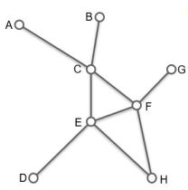
Figure 7: Small data instance

From/To	Train type	Num. trains	Start/End period	Possible links, $L_{r}^{P}$
A/H	freight	10	1/10	{A-C, C-E, E-H, C-F, F-H}
B/H	pax	25	3/11	{B-C, C-E, E-H, C-F, F-H}
D/G	freight	21	1/11	{D-E, E-F, F-G}
E/F	pax	19	3/11	{E-F}

Table 10: Traffic relations, small data instances

Link	$\nu_{l*,fr}$	$\nu_{l*,px}$	$C_{l*}$
A-C	0.3	0.2	5
B-C	0.2	0.1	5
C-E	0.2	0.1	5
C-F	0.2	0.1	5
E-H	0.3	0.2	5
F-H	0.4	0.3	5
D-E	0.3	0.2	5
E-F	0.2	0.1	5
F-G	0.2	0.1	5

Table 11: Train speed values and capacity settings

The aggregated train type variant exhibits substantial amount of flow mixing between the traffic relations (of the same train types) and we think that overcoming these issues by, for example, introduction of cuts or lazy constraints is not worth further investigation.

The multi-commodity variant solves these small instances correctly, but results in a larger problem size (see discussion in Section B.3). For these instances the solving time is negligible (<< 1 s) and with no noticeable difference in performance between the two formulations.

The primary result of these tests are that the method for calculating the share of flow within the same time period works reasonably well except for an important issue regarding spreading of fractional flow. In Table 12 the result for one of the traffic relations is presented, which shows the amount of flow that moves forward in time. We also note that for this small case the capacity restrictions are limiting (for links B-C, C-E, and E-H during time periods 6–8), as shown in Table 13, and that some train cancellations are necessary in order to find a feasible solution.

	Time period
	3	4	5	6	7	8	9	10	11	12
$x_{rt}^{O}$	1	1	3	5	5	5	3	1
B-C	0.9:0.1	0.9:0.1	2.7:0.3	4.5:0.5	4.5:0.5	4.5:0.5	2.7:0.3	0.9:0.1
C-E	0.8:0.1	0.9:0.1	2.5:–	4.2:–	4.2:–	4.2:–	2.9:–	1.1:0.1	0.1:–
E-H	0.6:0.2	0.8:0.2	2.1:0.6	3.3:0.9	3.3:0.9	3.3:0.9	2.3:0.6	0.9:0.2	0.2:0.0
C-F	–:–	–:–	–:0.3	0.1:0.5	0.3:0.5	0.3:0.5	–:0.3	–:–
F-H	–:–	–:–	–:–	0.4:0.0	0.7:0.1	0.7:0.1	0.5:–	0.3:–
$x_{rt}^{D}$	0.6	1.0	2.2	4.2	4.9	5	3.8	1.8	0.4	0.0

Table 12: Flow solution for traffic relation B/H (pax). Link flow values are given as $x_{ltr}^{Tr,d}$:$x_{ltr}^{Tr,n}$.

	Time period
Link	3	4	5	6	7	8	9	10	11	12
B-C	0.95	1.0	2.9	4.9	5.0	5.0	3.1	1.1	0.1
C-E	1.85	2.0	3.4	5.0	5.0	5.0	3.8	2.1	0.6
E-H	1.7	2.0	3.4	4.8	5.0	5.0	3.8	2.3	0.9	0.1
C-F			0.2	0.7	1.0	1.0	0.5	0.2
F-H				0.6	1.0	1.0	0.7	0.3

Table 13: Capacity usage. Capacity limitations marked with red text color.

The issue with small fractional flow volumes is not too problematic when the number of traversed links (for each traffic relation) is small. But as the number of links increase it becomes increasingly problematic. We have unsuccessfully tried to figure out some additional handling within the above variant of the multi-commodity formulation. Instead we have chosen to redefine the layering structure of the network so as to have one layer for each routing option of the traffic relations. The input data for flow shares within the same time period ($\nu$) is also extended so as to give the possible amount that can reach every node along the specific route. The model formulation for this is given in an accompanying document [2].

References

- [1] M. Aronsson “Transporttillgänglighet och tillgänglighetsnyckeltal för järnvägsnät och banunderhåll”, 2019 URL: http://urn.kb.se/resolve?urn=urn:nbn:se:ri:diva-38326
- [2] M. Aronsson and T. Lidén “A model for calculating volumes of trains as flows given demand and capacity restriction” SATT project subreport, 2021
- [3] M. Burkhalter “A novel methodology to optimise intervention programs for railway infrastructure networks in a digital environment”, 2021 DOI: 10.3929/ethz-b-000490172
- [4] W. Li and C. Zhang “A bi-objective optimization approach for the maintenance planning of networked systems” In Quality and Reliability Engineering International, 2020 DOI: 10.1002/qre.2633
- [5] T. Lidén, M. Aronsson and C. Liu “Samplanering av trafikpåverkande åtgärder och trafikflöden, modellstudie: Delrapport 1 – Krav- och behovsinventering”, 2021
- [6] T. Lidén, L. Brunsson and F. Lundström “Utformning av servicefönster för varierande trafik- och underhållssituationer”, 2020 URL: http://urn.kb.se/resolve?urn=urn:nbn:se:liu:diva-171742
- [7] T. Lidén and M. Joborn “An optimization model for integrated planning of railway traffic and network maintenance” In Transportation Research Part C: Emerging Technologies 74, 2017, pp. 327–347 DOI: 10.1016/j.trc.2016.11.016