Machine learning the 2D percolation model

Abstract

We use deep-learning strategies to study the 2D percolation model on a square lattice. We employ standard image recognition tools with a multi-layered convolutional neural network. We test how well these strategies can characterise densities and correlation lengths of percolation states and whether the essential role of the percolating cluster is recognised.

1 Introduction

A popular application of machine learning (ML) is the identification and classification of phases of matter [1, 2, 3, 4]. For example, many properties of the ferromagnetic-to-paramagnetic phase transition in the 2D Ising model were reconstructed in Ref. [2] while Anderson-type transitions and phase diagrams for models of topological matter have been considered in Ref. [5]. These promising results seem to pave the way for ML as a standard tool in condensed matter. ML approaches based on deep, i.e., multi-layered, neural nets fall into three broad classes namely, supervised, un-supervised and reinforcement learning approaches. Common to all approaches is the feed-forward/back-propagation cycle in which parameters of the neural nets are optimised such that suitably chosen loss functions become minimal. Various network architectures have been shown to be appropriate for tasks as varied as image recognition [6], deepfakes [7, 8] and board games [9]. Here, we shall employ supervised learning strategies in the 2D percolation model on a square lattice. It is well known that the percolation in 2D exhibits a phase transition as a function of occupation densities with a diverging two-point correlation length at a critical density $p_{c}$. Previous studies [4, 10] found supervised learning able to distinguish the two phases of the percolation model, while the utility of unsupervised learning seems less established [10, 11]. The aim of this paper is to develop a robust ML strategy to identify for finite lattices whether a given percolation lattice contains a spanning cluster or not. As such, we will (i) classify, with ML, percolation lattices according to densities and correlation lengths and (ii) use ML regression to predict densities and correlation lengths.

2 Model and Methods

The site percolation model on a 2D $L\times L$ lattice is defined as follows [12]: sites on the lattice are randomly occupied with probability $p$ and left empty with probability $1-p$. Each site has four neighbours, i.e., two along the horizontal and two along the vertical axes. A group of neighbouring occupied sites is called a cluster. For small $p$ values, most clusters have size $<L$ while for $p\rightarrow 1$, the cluster size tends to $L^{2}$. At the percolation threshold $p_{c}$ a spanning cluster emerges which connects opposite sides of the lattice. Much previous work [13, 12] has established that for $L\rightarrow\infty$, $p_{c}=0.59274605079210(2)$ [14]. For finite $L$, one usually finds upon averaging a threshold value $p_{c}(L)<p_{c}$. Numerically, the Hoshen-Kopelman cluster identification algorithm [15] allows for a determination of $p_{c}(L)$ while also giving full information about the cluster geometries and shapes. We use it to compute configurations $\psi_{n}(\mathbf{r})$ of occupied and empty sites on $100\times 100$ lattices with $20$ densities $p=0.1,0.2,\ldots,0.55,0.56,\ldots,0.66,0.7,\ldots,0.9$ and $N=5000$ samples for each density. Here, $n$ labels different configurations while $\mathbf{r}$ indicates positions of individual sites and $\psi_{n}(\mathbf{r})\in\{0,1\}$ denotes whether at $\mathbf{r}$ there is an empty ($0$) or occupied ($1$) site in the $n$ state. Examples of such $\psi_{n}$ are given in Fig. 1(a-c). Our results suggest that ${p_{c}}(100)\approx 0.59\pm 0.03$ for our data, computed with open boundary conditions. The transition from non-spanning clusters at $p<p_{c}$ to a spanning cluster at $p>p_{c}$ is a continuous phase transition with the probability $P(p)$ that an arbitrary site belongs to the infinite cluster acting as the order parameter. Similarly, the connected correlation function $g(r)$, defined as the probability of a site at distance $r$ from an occupied site to belong to the same cluster [16], diverges at $p_{c}$. Its associated correlation length $\xi=\sqrt{{\sum_{r}r^{2}g(r)}/{\sum_{r}g(r)}}$ gives the average distance between two sites that belong to the same cluster. As $p\rightarrow p_{c}$, $\xi\propto\mid p-p_{c}\mid^{-4/3}$ for $L\rightarrow\infty$. An example of the behaviour of $\xi(r)$ in our data is shown in Fig. 1(d) where we can see that $\xi$ indeed is maximal at ${p_{c}}(100)$ but does not diverge for the calculated $p$ values.

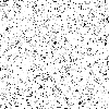
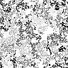
(a) (b) (c) (d)

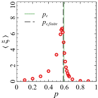
Figure 1: Percolation states on a $100\times 100$ lattice with open boundary conditions for (a) the non-percolating phase ($p=0.2<p_{c}$), (b) close to the transition ($p=0.5\approx p_{c}$) and (c) in the spanning phase ($p=0.6>p_{c}$). Different clusters of occupied sites are denoted by grey squares and identical grey levels indicate a common cluster. There are 1235, 597 and 248 clusters in (a), (b) and (c), resp., and the largest cluster size is 12, 252 and 4422, resp., in each panel. (d) Average correlation length $\langle\xi\rangle(p)$ computed from $5000$ percolation states for $20$ $p$ values and periodic boundaries. The vertical lines denote $p_{c}$ in the thermodynamic limit [14] (green dotted) and the position $p=0.5853$ for the largest $\langle\xi\rangle$ as a estimate of $p_{c}$ for our finite-sized systems (black dashed). The standard error of the mean for each data point is within symbol size.

Convolution neural nets (CNN) are a class of multi-layered (deep) neural nets in which spatial locality of data values is retained during the ML training. When coupled with a form of residual learning [17], the resulting residual networks (ResNets) have been shown to allow astonishing precision when classifying images, e.g., of animals [18] and handwritten characters [19], or when predicting numerical values, e.g., of market prices [20]. Here, we shall use a ResNet18 [17] network with $17$ convolutional and $1$ fully-connected layers, pretrained on the ImageNet dataset [21]. For our implementation we use the PyTorch suite of ML codes [22]. We train the ResNet18 on the $\psi_{n}$ configurations, using a $90\%$/$10\%$ split into training and validation data. Additional $\psi_{n}$ configurations are generated as necessary for test runs. We concentrate on two ML tasks. First, we classify percolation configurations $\psi_{n}$ according to densities $p$, correlation lengths $\xi$ and spanning non-spanning. In the second task, we aim to predict $p$ and $\xi$ values via ML regression. In both problems, the overall network architecture remains identical, we just adapt the last layer. For the classification the output layers have a number of neurons corresponding to the number of classes trained i.e, for the classification by density the ${\cal C}=20$ values $p=0.1,0.2,\ldots,0.55,0.56,\ldots,0.66,0.7,0.8,0.9$, while for regression the output layer has only one neuron making the predictions. However, the loss functions are different. Let $\omega$ denote the parameters (weights) of the ResNet and let $(\psi_{n},\chi_{n})$ represent a given data sample with $\chi_{n}$ the classification/regression targets, i.e., classes $p$ or $\xi$, and also ${\chi}^{\prime}_{n}$ the predicted values, $p^{\prime}$ or $\xi^{\prime}$. For classification of categorical data, the class names are denoted by a class index $a=1,\ldots,{\cal C}$ and encoded as $\chi_{ai}=1$ if $\chi_{ai}=i$, $0$ otherwise. Then, for the (multi-class) classification problem, we choose the usual cross-entropy loss function, $\l_{\mathrm{c}}(\omega)=-\sum_{i=1}^{N{\cal C}}\sum_{a=1}^{{\cal C}}\chi_{ai}\log{\chi^{\prime}}_{ai}(\omega)+(1-\chi_{ai})\log[1-\chi_{ai}(\omega)]$ [23]. On the other hand, the loss function for the regression problem is given by the mean-squared error $l_{\mathrm{r}}(w)=\frac{1}{n}\sum_{i=1}^{N{\cal C}}[\chi_{i}-{\chi}^{\prime}_{i}(w)]^{2}$. When giving results for the values of the loss functions below, we always present those after averaging over at least $10$ independent training and validation cycles. We also represent the quality of a prediction by confusion matrices [23]. These graphically represent the predicted class labels as a function of the true ones in matrix form, with an error-free prediction corresponding to a diagonal matrix. For comparison of the classification and regression calculations, we use in both cases a maximum number of $\epsilon_{\mathrm{max}}=20$ epochs. Our ML calculations train with a batch size of $16$ for classification and for regression on an NVIDIA Quadro RTX 6000 GPU card.

3 Results

Figure 2(a) shows the training and validation losses for classifying densities.

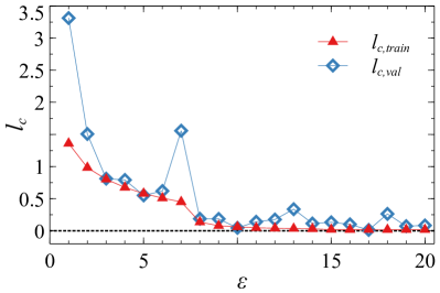
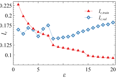
(a)         (b)
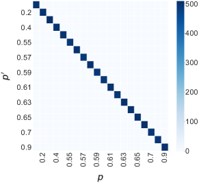
(c)        (d)
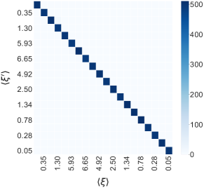
(e)        (f)

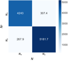
Figure 2: (a,c,e) Dependence of losses $l_{\mathrm{c,train}}$ and $l_{\mathrm{c,val}}$ on the number of epochs $\epsilon$ for classification according to (a) $p$’s, (c) $\xi$’s and (e) spanning/non-spanning. The diamonds (blue open) denote $l_{\mathrm{c,train}}$ while the triangles (red solid) show $l_{\mathrm{c,val}}$. The thin lines are guides to the eye only. The horizontal dotted lines in (a,c) indicate $l_{\mathrm{c}}=0.$ (b,d,f) Confusion matrices for the validation data used in (a,c,e) at $\epsilon=20$. The true labels for $p$, $\xi$ and $N_{s}$/$N_{n}$ are indicated on the horizontal axes while the predicted labels are given on the vertical axes. The colour scale represents the number of samples in each matrix entry, for (f) these are given explicitly.

An excellent training result is corroborated by a perfectly diagonal confusion matrix shown in Fig. 2(b). We note that this also holds when the spacing of densities is reduced as for the values $p=0.55,0.56,\ldots,0.66$ around $p_{c}$. We now repeat the procedure of classification, but replace the density $p$ labels with the computed average correlation lengths, $\langle\xi(p)\rangle$. These are $\langle\xi(0.1)\rangle,\langle\xi(0.2)\rangle,\ldots,\langle\xi(0.9)\rangle$ corresponding to $0.18\pm 0.07$, $0.35\pm 0.07$, $0.65\pm 0.05$, $1.30\pm 0.05$, $3.36\pm 0.07$, $5.93\pm 0.06$, $6.48\pm 0.04$, $6.65\pm 0.07$, $6.18\pm 0.05$, $4.92\pm 0.04$, $3.56\pm 0.06$, $2.50\pm 0.03$, $1.78\pm 0.05$, $1.34\pm 0.07$, $1.01\pm 0.07$, $0.78\pm 0.05$, $0.62\pm 0.04$, $0.28\pm 0.04$, $0.08\pm 0.07$, $0.05\pm 0.05$, respectively, in Fig. 1(d). In Figs. 2(c, d) we show $l_{\mathrm{c,train}}(\epsilon)$, $l_{\mathrm{c,val}}(\epsilon)$ and the confusion matrix, respectively. We again use the full set of $20$ classes for the classification. As we can see in Fig. 2(c), the loss for the classification is as good as for the density classification shown in Fig. 2(a). Of course this should not be surprising since we effectively just replaced the $p$ labels with $\xi$ labels.

The percolation transition distinguishes non-spanning clusters at $p<p_{c}$ from spanning clusters at $p\geq p_{c}$. We therefore now also train the ResNet with all percolation data, but just using their classification in non-spanning and spanning percolation clusters as labels. In Figs. 2(e) and (f) we show $l_{\mathrm{c,train}}(\epsilon)$, $l_{\mathrm{c,val}}(\epsilon)$ and the confusion matrix, respectively. The confusion matrix shows good recognition for the majority of cases. Nevertheless, we also see that about $5\%$ of the samples get misclassified, i.e., $298$ of $4565$ non-spanning clusters are classified as spanning while $279$ of $5434$ spanning clusters are wrongly identified as non-spanning. This suggests that the classification routine is struggling with correctly identifying the spanning cluster.

The classification approach is in principle restricted in its predictive accuracy for $p$ by the number of available classes. While one can of course try to increase the number of classes, this will also lead to an increased chance in misclassifying percolation states from close by classes. The regression method outlined in section 2 allows to predict the $p$ value for a given percolation state directly. We again start from a pre-trained ResNet in Fig. 3(a) we show the training and validation losses, $l_{\mathrm{r,train}}$ and $l_{\mathrm{r,val}}$, respectively.

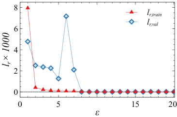
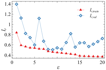
(a)      (b)
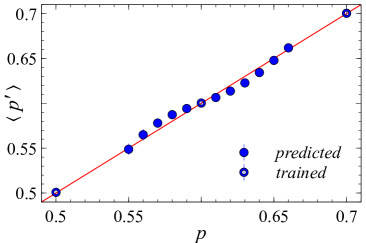
(c)      (d)

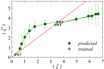
Figure 3: (a,c) Dependence of $l_{\mathrm{r,train}}$ and $l_{\mathrm{r,val}}$ on $\epsilon$ for the regression task with (a) $p$’s and (c) $\xi$’s. Similar to Fig. 2, triangles denote $l_{\mathrm{r,train}}$ and diamonds show $l_{\mathrm{r,val}}$. Lines are as before. (b, d) Dependence of the true (b) $p$ on $p^{\prime}$ and (d) $\xi$ on $\xi$’. The red lines denotes the perfect predictions $p=p^{\prime}$ and $\langle\xi\rangle=\langle\xi\rangle^{\prime}$. The three open circles highlight (c) $p=0.5$, $0.6$ and $0.7$ and, respectively, (d) $\langle\xi\rangle=3.36\pm 0.07$, $3.56\pm 0.06$ and $0.28\pm 0.04$ included in the training sets while the solid circles are the results of the regression.

We train the ResNet for the evenly-spaced $9$ densities $p=0.1,0.2,\ldots,0.9$. We then use the data from the $12$ densities $p=0.55,0.56,\ldots,0.66$ as test of the regression model. We note that in this approach, the $p=0.6$ data is used both in the training/validation cycle as well as in the test. In Fig. 3(b) we show the dependence of the true density $p$ as a function of the average predicted density $p^{\prime}$. We see that the predicted $p^{\prime}$ values closely follow the true $p$’s. However, we also find that the predictions cluster somewhat around $p=0.6$, a $p$ value used in the training.

We can also perform a regression study using the correlation lengths $\xi$ as regression target. However, we now have a distribution of computed $\xi$ values for each $p$ whereas for $p$-regression, each sample has exactly the correct $p$ value. For a given $p$ value, we therefore construct an average value $\langle\xi\rangle$. In order to capture this behaviour correctly, we train our ResNet on the individual $\xi$ values for each sample at given $p$. Similarly, when computing the predicted $\xi^{\prime}$ values, we average the individual predictions for given $p$ to construct $\langle\xi^{\prime}\rangle$. As before for $p$ regression, we train using the $\xi$ values of the percolation states for densities $p=0.1,0.2,\ldots,0.9$ and predict $\xi^{\prime}$ from the $12$ densities $p=0.55,0.56,\ldots,0.66$. While all the previous training were performed on percolation states where empty sites were denoted by 0 and occupied site by 1, this dataset did not provide exploitable results. We therefore decided to train with percolation states containing the numbered cluster found through the Hoshen-Kopelman algorithm [15]. We obtain the dependence of the average predicted label $\langle\xi^{\prime}\rangle$ on the average true label $\langle\xi\rangle$ as shown in Fig. 3(d). In Fig.  3(b), we see that there are important deviations from a perfect regression curve $\langle\xi^{\prime}\rangle=\langle\xi\ \rangle$ with $\langle\xi\rangle$ corresponding to trained configuration $p=0.5$, $p=0.6$ and $p=0.7$ on the line of perfect regression.

4 Conclusions

We have shown that CNNs, and in particular pretrained ResNets, are able to successfully classify percolation states according to densities $p$ and correlation lengths $\xi$ in the case of the 2D site percolation on a square lattice. When trying to classify spanning versus non-spanning percolation states, the results are less convincing. While the majority of samples are being correctly classified, there are about $5\%$ of percolation states which are wrongly classified. This suggests that the ResNet is not able to identify the percolating/non-percolating nature of clusters correctly. For the regression analysis, when trained with evenly spaced densities $p=0.1$, $0.2$, $\ldots$, $0.9$, we find good quantitative predictions, even for much closer spaced densities $p=0.55$, $0.56$, $\ldots$, $0.66$. For the correlation length, the classification gave us perfect classes predictions, but the regression analysis showed that the network might not understand and therefore predict correctly correlation lengths.

In order to make sense of these results, one might want to ask whether the ML image recognition tools employed here simply count the number of occupied and unoccupied sites while disregarding the existing of a percolating cluster. Clearly, this would be consistent with the precision of the classification and regression results for $p$ and $\xi$. However, then we would not expect, e.g., the deviations from $p=p^{\prime}$ and $\xi=\xi^{\prime}$ seen in Fig. 3(b,d). Similarly, when looking at which clusters are wrongly classified during the spanning/non-spanning classification, we find that these are mostly spanning for $p\lesssim p_{c}$ and non-spanning for $p\gtrsim p_{c}$. Clearly, more studies are needed to clarify these issues.

References

References

- [1] Venderley J, Khemani V and Kim E A 2018 Phys. Rev. Lett. 120 257204 URL https://doi.org/10.1103/PhysRevLett.120.257204
- [2] Carrasquilla J and Melko R G 2017 Nat. Phys. 13 431–434 URL https://doi.org/10.1038/nphys4035
- [3] Ch’ng K, Carrasquilla J, Melko R G and Khatami E 2017 Phys. Rev. X 7 031038 URL https://doi.org/10.1103/PhysRevX.7.031038
- [4] Zhang W, Liu J and Wei T C 2019 Phys. Rev. E 99(3) 032142 URL https://doi.org/10.1103/PhysRevE.99.032142
- [5] Ohtsuki T and Mano T 2020 J. Phys. Soc. Jpn. 89 022001 URL https://doi.org/10.7566/JPSJ.89.022001
- [6] Fujiyoshi H, Hirakawa T and Yamashita T 2019 IATSS Research 43 244–252 URL https://doi.org/10.1016/j.iatssr.2019.11.008
- [7] Westerlund M 2019 TIM Review 9 40–53 URL http://doi.org/10.22215/timreview/1282
- [8] Karras T, Laine S, Aittala M, Hellsten J, Lehtinen J and Aila T 2020 Analyzing and improving the image quality of stylegan 2020 IEEE/CVF Conference on Computer Vision and Pattern Recognition (CVPR) pp 8107–8116 URL http://doi.org/10.1109/CVPR42600.2020.00813
- [9] Silver D, et al., 2017 Nature 550 354–359 URL https://doi.org/10.1038/nature24270
- [10] Cheng S, He F, Zhang H, Zhu K D and Shi Y 2021 Machine learning percolation model (Preprint 2101.08928)
- [11] Yu W and Lyu P 2020 Physica A 559 125065 URL https://doi.org/10.1016/j.physa.2020.125065
- [12] Stauffer D and Aharony A 1992 Introduction To Percolation Theory (Taylor & Francis) ISBN 9781482272376 URL https://www.taylorfrancis.com/books/9781482272376
- [13] Newman M E J and Ziff R M 2000 Phys. Rev. Lett. 85 4104–4107 URL https://doi.org/10.1103/PhysRevLett.85.4104; ibid, 2001 Phys. Rev. E 64 016706 URL https://doi.org/10.1103/PhysRevE.64.016706
- [14] Jacobsen J 2015 J. Phys. A Math. Theor. 48 URL https://doi.org/10.1088/1751-8113/48/45/454003
- [15] Hoshen J and Kopelman R 1976 Phys. Rev. B 14 3438–3445 URL https://doi.org/10.1103/PhysRevB.14.3438
- [16] Zhang J, Zhang B, Xu J, Zhang W and Deng Y 2021 Machine learning for percolation utilizing auxiliary Ising variables (Preprint 2110.06776)
- [17] He K, Zhang X, Ren S and Sun J 2016 2016 IEEE Conference on Computer Vision and Pattern Recognition (CVPR) 770–778 URL https://doi.org/10.1109/CVPR.2016.90
- [18] Tabak M A et al. 2019 Methods Ecol. Evol. 10 585–590 URL https://doi.org/10.1111/2041-210X.13120
- [19] Zhang R, Wang Q and Lu Y 2017 2017 14th IAPR International Conference on Document Analysis and Recognition (ICDAR) 05 25–29 URL http://doi.org/10.1109/ICDAR.2017.324
- [20] Zhao Y and Khushi M 2020 2020 International Conference on Data Mining Workshops (ICDMW) 385–391 URL http://doi.org/10.1109/ICDMW51313.2020.00060
- [21] Deng J, Dong W, Socher R, Li L J, Li K and Fei-Fei L 2009 ImageNet: A Large-Scale Hierarchical Image Database CVPR09
- [22] Paszke A et al. 2019 Pytorch: An imperative style, high-performance deep learning library Advances in Neural Information Processing Systems 32 ed Wallach H, et al. (Curran Associates, Inc.) pp 8024–8035 URL http://papers.neurips.cc/paper/9015-pytorch-an-imperative-style-high-performance-deep-learning-library.pdf
- [23] Mehta P, Bukov M, Wang C H, Day A G R, Richardson C, Fisher C K and Schwab D J 2019 Phys. Rep. 810 1–124 URL https://doi.org/10.1016/j.physrep.2019.03.001