VaxNeRF: Revisiting the Classic for Voxel-Accelerated Neural Radiance Field

Abstract

Neural Radiance Field (NeRF) is a popular method in data-driven 3D reconstruction. Given its simplicity and high quality rendering, many NeRF applications are being developed. However, NeRF’s big limitation is its slow speed. Many attempts are made to speeding up NeRF training and inference, including intricate code-level optimization and caching, use of sophisticated data structures, and amortization through multi-task and meta learning. In this work, we revisit the basic building blocks of NeRF through the lens of classic techniques before NeRF. We propose Voxel-Accelearated NeRF (VaxNeRF), integrating NeRF with visual hull, a classic 3D reconstruction technique only requiring binary foreground-background pixel labels per image. Visual hull, which can be optimized in about 10 seconds, can provide coarse in-out field separation to omit substantial amounts of network evaluations in NeRF. We provide a clean fully-pythonic, JAX-based implementation on the popular JaxNeRF codebase, consisting of only about 30 lines of code changes and a modular visual hull subroutine, and achieve about 2-8x faster learning on top of the highly-performative JaxNeRF baseline with zero degradation in rendering quality. With sufficient compute, this effectively brings down full NeRF training from hours to 30 minutes. We hope VaxNeRF – a careful combination of a classic technique with a deep method (that arguably replaced it) – can empower and accelerate new NeRF extensions and applications, with its simplicity, portability, and reliable performance gains. Codes are available at https://github.com/naruya/VaxNeRF.

1 Introduction

(a) NeRF

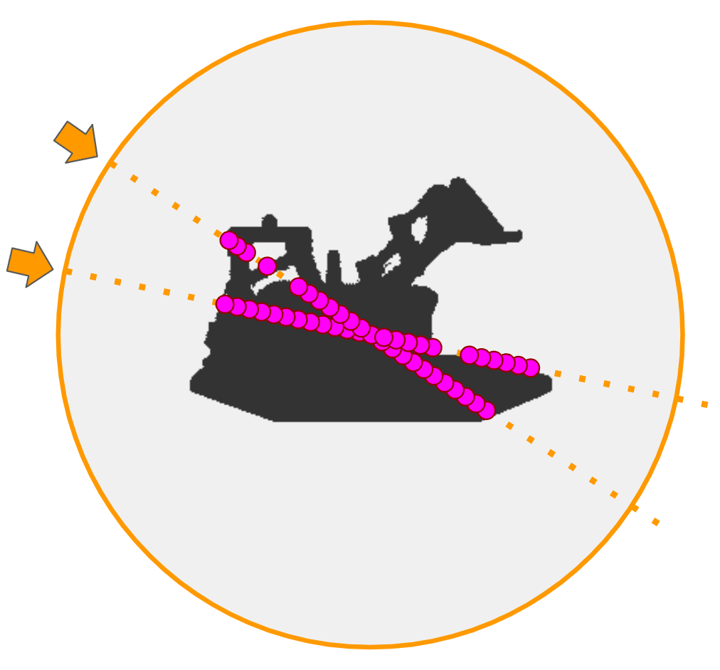
(b) VaxNeRF

Figure 1: NeRF (a) uses hierarchical sampling, i.e., a mixture of coarse (pink) and fine (light blue) sampling, to estimate the color from a specified viewpoint. Instead, VaxNeRF (b) samples only the inside of the bounding volume uniformly and densely. The orange circle shows the area bounded by the minimum and maximum distances of the rays, and the black shade in (b) shows the automatically obtained bounding volume.

Neural radiance field (NeRF) [41] has revolutionized high-resolution 3D reconstruction from images. Many extensions and applications quickly ensued, including dynamic scene rendering [31, 16, 67, 47, 51, 50], controllable relighting [3, 61, 77, 87], latent appearance and shape priors [57, 6, 68], scene composition [45, 21, 49, 79], and pose estimation [82, 62, 38, 32, 24].

These works have potential to make substantial impacts not only in computer vision and computer graphics, but also in robotics [30, 1], virtual reality (VR) systems [4, 23, 72, 42], and medical imaging [71].

Despite NeRF’s high quality 3D renderings, a key bottleneck has been slow training and inference speeds where the original implementation took days to render an object and tens of seconds to render a view angle [41]. Given this, follow up work looked to accelerate NeRF, including caching with special data structures [22, 18, 84], amortization through meta learning and multi-task learning [66, 2], or re-implementation optimized for parallel computing [54, 12], where most approaches focus on inference time speedups [54, 22, 18, 84, 34]. Notably, many of these approaches take NeRF as given and add extra complexities to enhance its performances, rather than fundamentally changing its design details, except a few [86, 34, 35].

Importantly, prior to NeRF there were many kinds of classic 3D reconstruction techniques [28, 55, 56, 76]. Instead of taking NeRF for granted and training end-to-end models, we revisit the basic building blocks of NeRF and ask: can classic techniques be combined with NeRF in meaningful ways? In this work, we focus on the points sampling in ray-color integration, which is a fundamental bottleneck to NeRF’s speed and is generally addressed through hierarchical sampling with coarse and fine models [41]. Visual hull [28], a classic 3D reconstruction technique, can obtain an approximate bounding volume, with only a binary foreground-background segmentation mask per image, which is easily obtainable through thresholding or recent off-the-shelf segmentation models [33, 19, 64]. Visual hull can be fitted for 100 images in about 10 seconds, using our JAX-based implementation, and using this coarse voxel model, we can eliminate most of the expensive point evaluations that are not inside the object. We term our method Voxel-Accelerated NeRF (VaxNeRF), which can eliminate the need for an extra coarse model, and can provide a consistent 2-8x faster training speedup on top of the highly-performative JaxNeRF [12] with a portable JAX-based visual hull file and only around 30 lines of modification to the main code.

We perform extensive evaluations using NeRF-Synthetic datasets, along with more difficult datasets of NSVF [35], to ensure that our observed speedups are consistent across various scenes without degradation in the final rendering quality (measured with PSNR and SSIM). We emphasize those scenes with non-convexities or transparencies, where visual hull alone certainly cannot provide ground-truth in-out volumes, but still observe that VaxNeRF provides similar degrees of speedups. On average VaxNeRF speeds up (Jax)NeRF training by 2-8x, with the same and sometimes higher final rendering accuracy. To our surprise, VaxNeRF, despite being a much simpler method to implement on top of NeRF or NeRF-based algorithms, also outperforms recent NSVF [35], as well as PlenOctrees [84] with respect to PSNRs, while providing better or comparable training speeds.

We hope that VaxNeRF, with its simplicity, portability, and reliable performance gains, can accelerate and empower many future NeRF extensions and applications. Extrapolating on the 256-TPU performance reported on JaxNeRF [12], VaxNeRF brings down full NeRF training from 2.5 hours to 30 minutes, only requiring additional binary foreground-background pixel labels. Our method, which simply combines a classic technique with a recent end-to-end technique, demonstrates the importance of revisiting core building blocks of popular deep learning models as well as classical techniques prior to them, as sometimes, the best of both worlds is a careful combination of the two.

2 Related Works

2.1 Novel View Synthesis

The task of synthesizing novel views of a scene given multiple images has been well studied for a long time, with various methods that divide into two categories: 3D reconstruction methods and viewpoint interpolation methods.

3D Reconstruction

The voxel-based methods [28, 27, 59] are very primitive methods for 3D reconstruction, which infer the occupancy or color of each point in grid space using the silhouette of the image or the viewpoint invariances of the color. Along with voxel representation, meshes are another commonly used representation[39, 5, 10, 78] since they are easy to use and can store information efficiently, but it is difficult to capture or optimize detailed geometry and topologies. MVS [25, 70] is an example of practical applications of 3D reconstruction form images, and is commonly used in 3D modeling work today. Recently, several deep learning-based approaches are proposed to continuously represent the 3D space  [37, 68, 80, 41]. Neural Volumes [37] performs 3D reconstruction by 3D deconvolution from accumulated image features, and then synthesize image from novel views by ray marching. Similarly, NeRF[41] uses ray marching, but instead of using 3D deconvolution, it learns a model that infers color and density given the coordinates and viewing direction along the camera ray. NSVF [35] is akin to a combination of NeRF and Neural Volumes, and speeds up the inference of NeRF by allowing features to be stored in a voxel grid. And lastly, there are other methods of 3D reconstruction using implicit functions such as the signed distance function  [80, 68].

Viewpoint Interpolation

Multi plane images [88, 69] and light field interpolation [9, 29, 20, 40] are image-based approaches for novel view synthesis without 3D reconstruction. When the postures of novel viewpoints can be limited, such as forward-facing scenes, these representations are very light-weight, accurate and effective, but otherwise, their use case is limited. Additionally, there are novel view synthesis methods use convolution-based deep generative models[14, 44]. While these are good at generating photo-realistic images at a reasonable speed, they have a problem that the geometry are prone to collapsing.

2.2 NeRF Accelerations

NeRF is attractive because of its ability to learn and represent precise shapes and complex reflections. However, NeRF’s training and inference (rendering) speed are very slow [41]. Many researchers have proposed methodologies to overcome this problem.  [84, 18, 22, 54, 53] are great methods for speeding up the NeRF inference. While the original NeRF took about 30 seconds to render one image, these methods achieve real-time rendering by pre-computing and storing colors and densities in scene space, or by dividing the NeRF model into smaller models for better parallel inference. Another way to speeding up NeRF on a new scene is to incorporate priors learned from a dataset of similar scenes, which can be accomplished by conditioning on predicted images features  [68, 85, 74, 7] or meta-learning  [66]. While these methods are effective for simple scenes or rough 3D reconstructions, these are not yet able to be used to generate complex scenes in the NeRF paper to the same quality. TermiNeRF [52] is a more direct way to speed up NeRF, where along with the usual NeRF model, it simultaneously trains a sampling network that predicts the locations of points to be sampled on a ray. Although it is claimed to speed up fine-tuning to a scene with the same shape but different look and lighting that has been learned once, it does not mention speeding up training itself. AutoInt[34] modifies the architecture of the NeRF to be able to calculate color and density by definite integration, however, the learning speedup is limited to 1.8x. Another approach for speeding up is to focus only on the object surfaces for 3D reconstruction and rendering [48, 73, 83, 81, 48], but it is extremely difficult to correctly estimate the shapes for objects with transparent parts or fuzzy objects whose surface is difficult to estimate. Our method, on the other hand, achieves faster training without narrowing down applicable domains or sacrificing rendering quality.

	fast rendering	fast training	quality	transparency	depth	representation	code modification
NeRF [41]	($\approx$ 0.05fps)	—	Good	Yes	No	NR	—
KiloNeRF [54]	$\approx$ 1000x	N/A	$\sim$ Good	Yes	No	NR	1000s+
SNeRG [22]	$\approx$ 1600x	N/A	$\sim$ Good	Yes	No	NR + Cache	1000s+
FastNeRF [18]	$\approx$ 4000x	N/A	$\sim$ Good	Yes	No	Cache	1000s+
PlenOctrees [84]	$\approx$ 3000x	$\approx$ 4x	$\sim$ Good	Yes	No	SH	$\approx$ 1000s
NSVF [35]	$\approx$ 10x	N/A	Good	Yes	No	NR	1000s+
AutoInt [34]	$\approx$ 10x	$\approx$ 1.8x	Lower	Yes	No	NR	1000s+
TermiNeRF [52]	$\approx$ 14x	N/A	Good	Yes	No	NR	unknown
MetaNLR [2]	$\approx$ 20x	$\approx$ 8x	$\sim$ Good	No	No	NR	unknown
DoNeRF [43]	15-78x	$\approx$ 6x	Good	Yes	Required	NR	1000s+
DS-NeRF [13]	N/A	2-6x	$\sim$ Good	Yes	Required	NR	1000s+
VaxNeRF (Ours)	N/A	2-8x	Good	Yes	No	NR	$\approx$ 30

Table 1: A comparison of efficient NeRF-based methods. fast rendering and fast training: How many times faster the rendering / training are compared to NeRF. “No” does not mean no speedup at all, but indicates that it is not specifically mentioned in the paper. quality: Rough quality comparison with NeRF as “Good”. The “ Good” indicates that the quality depends on parameters such as compression ratio. transparency: Whether the method can handle objects that cannot be successfully reconstructed by simply estimating the object’s surface (e.g. objects with transparency). depth: Whether a depth image is required. representation: The representation of the model that will eventually be created by each method. “NR” denotes neural representation, “cache” denotes the precomputed values of color and density, and “SH” denotes the coefficient of spherical harmonics. code modification: How many lines have been changed/add from the original NeRF implementation. If the code has not been published, displayed as “unknown”.

2.3 NeRF and 3D Geometry Integration

There are several work that expand NeRF using geometry data inferred from images or given as a supervised information.  [75, 46] use a rough bounding volume obtained from visual hull [28] to measure occupancy loss to get a clear estimate of the object surface, but they do not focus on obtaining significant speed-ups. NeLF [63] is an intricate, highly-customized method for portrait view synthesis that combines NeRF and NeuralVolumes. NeLF uses visual hull to reduce the number of sampling points on a ray, but does not study how effective it is alone or in the most basic form of NeRF. NeuRays [36] is an image-based rendering method that utilizes the surface information of objects obtained by Colmap [56, 55]. DoNeRF [43] and DS-NeRF [13] use depth images to reduce the number of required observation images and speed up training, but our method achieves faster training without such depth oracle.

3 Preliminaries

Our work builds on the most basic NeRF model with minimal changes. We go over the NeRF basics and introduce visual hull in this section. For more in-depth summaries of NeRFs and extensions, please refer to [11].

3.1 Neural Radiance Fields

Neural radiance fields (NeRF) [41] are 3D representations that can be rendered from arbitrary viewpoints, capturing continuous geometry and view-dependent appearances. The expected color of a camera ray $\mathbf{r}(t)=\mathbf{o}+t\mathbf{d}$ can be estimated by a finite-sample approximation $\hat{C}(\mathbf{r})$:

$$\hat{C}(\mathbf{r}) =\sum_{i=0}^{N-1}w_{i}\,\mathbf{c}(\mathbf{r}(t_{i}))\,,$$ (1)

$$\text{where}\quad w_{i} =T_{i}\big{(}1-\exp(-\mathbf{\sigma}(\mathbf{r}(t_{i}))\delta_{i})\big{)}$$ (2)

$$T_{i} =\exp\left(-\sum_{j=0}^{i-1}\mathbf{\sigma}(\mathbf{r}(t_{j}))\delta_{j}\right),$$ (3)

where $t_{i}$ indicates the position of the point to be sampled from the ray, and $\delta_{i}=t_{t+1}-t_{i}$ are the distances between point samples.

In NeRF, an MLP parameterizes $\mathbf{c}(\cdot)$ and $\mathbf{\sigma}(\cdot)$ jointly and is trained to minimize the loss between the ground-truth pixel colors $C(\mathbf{r})$ in the images and the predicted colors $\hat{C}$ for a batch of rays $\mathcal{R}$:

$$\mathcal{L}_{\text{RGB}}=\sum_{\mathbf{r}\in\mathcal{\mathcal{R}}}\big{\lVert}{C(\mathbf{r})-\hat{C}(\mathbf{r})}\big{\rVert}^{2}_{2}$$ (4)

Hierarchical Sampling

The NeRF paper [41] proposes hierarchical sampling to efficiently determine the points $t_{i}$ to be evaluated for each ray in Eq. 1. Two NeRF models with the same network structure are trained jointly: a coarse model and a fine model. For the coarse model the points $t_{i}$ are sampled uniformly, while for the fine model $t_{i}$ are sampled from an importance-weighted distribution based on their contributions $w_{i}$ to the final pixel value $\hat{C}$, evaluated using the coarse model. 1(a) visually shows how the fine model can better allocate samples to important regions, leading to much lower PSNR.

3.2 Visual Hull

Visual hull [28] (or shape-from-silhouette) is a classical method for 3D reconstruction based on a set of images and their camera location information. It assumes that pixels in each captured image can be divided into foreground and background.

The foreground region of an image is created by the projection of a three-dimensional object onto a two-dimensional plane. Therefore, we know that there is absolutely no object on the ray of the camera corresponding to a pixel in the background region, and conversely, there is always an object somewhere on the ray corresponding to a pixel in the foreground region. Therefore, we can narrow down the area where an object may be present using a set of images from multiple angles, and the product of the possible areas where an object is present in each image forms an approximate bounding volume of (a region that completely contains) the object.

Visual hull is a primitive method, and has problems such as inability to correctly restore (carve off) some dented parts of non-convex shapes, but unlike other methods [27, 59, 7, 58, 60, 15, 17], it has the advantage of being able to obtain a bounding volume that contains 100% of the object and therefore has been applied in many ways in classic 3D reconstructions [65, 26, 20].

While visual hull is a method for estimating shapes and not colors, it can be easily colored by shooting rays from the foreground of the given image to the output voxels of the visual hull. For visualization, we present a colored output of the visual hull in Figure 3, but we did not use this color information in our method.

4 Method

An obvious yet significant compute inefficiency in NeRF training is its MLP evaluations at the points in space where they have no object and contribute $0$ to $\hat{C}(\mathbf{r})$. While NeRF addresses this by training a separate coarse model for point selections, we propose a simpler solution: we modify Eq. 1 to only evaluate the points inside of the voxels $\mathcal{V}$ created by visual hull,

$$\hat{C}(\mathbf{r}) =\sum_{i:\mathbf{r}(t_{i})\in\mathcal{V}}w_{i}\,\mathbf{c}(\mathbf{r}(t_{i})).$$ (5)

We term it Voxel-Accelerated NeRF (VaxNeRF). While this is arguably a trivial and intuitive modification to NeRF, VaxNeRF has the following advantages over standard NeRF or other accelerated-NeRF variants:

• It is implementable on top of JaxNeRF [12] in about 30 lines, fully pythonic and JAX-based (Figure 2)

• It trains 2-8x faster than JaxNeRF

• It trains without loss of rendering quality measured in PSNR and SSIM

• It trains only one network for best performance, as opposed to two in NeRF

where the only additional assumption is the access to binary foreground-background masks, which are easily obtainable in most cases as discussed in Section 5.1. We show how this simple combination of a well-known classical technique and NeRF leads to these impressive empirical performances in Section 5.2 (Figure 3, Figure 4, Table 2, Table 3).

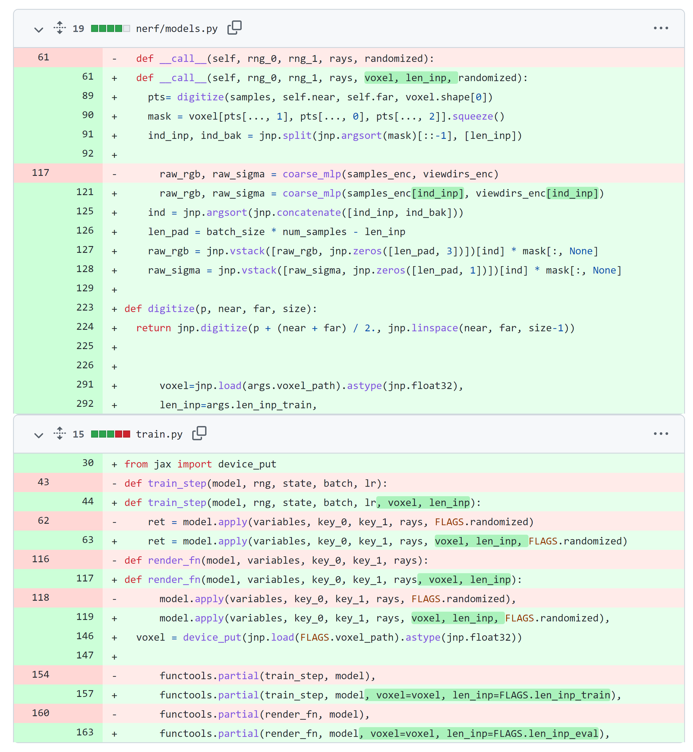
Figure 2: The full code modification to convert from (Jax)NeRF [41, 12] to VaxNeRF, visualized with “git diff”. This is not for readability (for algorithmic differences, see Algorithm 1), but mainly for highlighting how it only takes about 30 lines of change to implement VaxNeRF and achieve the speedups, besides a modular visual hull code.

4.1 Design Choices

Despite the simplicity and generality of the core VaxNeRF idea, there were a number of key design decisions in VaxNeRF implementation to achieve the best performances.

Choosing visual hull

As noted briefly in Section 3.2, visual hull is reliable: it only undercuts spaces (e.g. fail to cut dents in objects), but never overcuts. This property is critical in VaxNeRF, since as long as all object parts are inside $\mathcal{V}$, it will converge to the same performance as a full NeRF. In Colmap [55, 56] and photogrammetry [76], on the other hand, the object surface is estimated using color information that is vulnerable to reflections and other noise, and the estimated surface contains noise and is not suited to be a reliable bounding volume, unlike in visual hull where the estimated volume is 100% reliable up to the resolution of voxels. We therefore chose visual hull to derive $\mathcal{V}$ used in VaxNeRF.

Removing fine model

As illustrated in Figure 1, $\mathcal{V}$ in VaxNeRF decides point locations based on a binary bounding volume, and the fine model in NeRF decides based on a more direct measure of contribution to the ray color $\hat{C}(\mathbf{r})$, i.e. $w_{i}$, evaluated through the coarse model. Visually it appears that using the fine model of NeRF on top of VaxNeRF could lead to even more speedups; however, through our extensive experiments we found that VaxNeRF performs the best using only a single “coarse” model with (dense) uniformly sampling (e.g. Figure 4). This removes the need for fine model and substantially simplifies NeRF training.

Dilating voxels

NeRF usually uses 64 and 128 points for coarse and fine sampling respectively [41], while our visual hull constructs 400x400x400 voxels. This means that if there is a substructure in the scene that is smaller than 1/64 of the scene size, the ray may ignore that part of the scene even if visual hull was able to reconstruct it. In order to avoid this problem, we dilate, i.e. max-pool, the voxel by the amount of cells equal to the scene size divided by the number of point samples, when the sample size is small, e.g. 64.

5 Experiments

Synthetic NeRF Dataset     best second-best third-best
	0.5h		1h		3h		6h		12h		36h
Method	PSNR	SSIM	PSNR	SSIM	PSNR	SSIM	PSNR	SSIM	PSNR	SSIM	PSNR	SSIM
c64f64	27.07	0.908	28.64	0.926	29.98	0.939	30.73	0.946	31.22	0.949	31.39	0.951
c64f128	26.66	0.903	28.36	0.923	29.96	0.939	30.75	0.946	31.4	0.951	31.73	0.953
vax_c64f64	29.33	0.932	30.07	0.939	31.1	0.948	31.38	0.95	31.43	0.951	31.43	0.951
vax_c64f128	28.82	0.927	29.78	0.937	31.03	0.947	31.53	0.951	31.71	0.953	31.73	0.953
vax_c400	30.04	0.939	30.73	0.945	31.35	0.95	31.43	0.951	31.44	0.951	31.44	0.951
vax_c600	30.0	0.938	30.8	0.945	31.72	0.952	31.92	0.954	31.95	0.955	31.95	0.955
vax_c800	29.8	0.936	30.69	0.944	31.78	0.953	32.1	0.955	32.17	0.956	32.18	0.956
nsvf	24.96	0.875	26.04	0.893	26.91	0.908	27.52	0.92	28.04	0.93	28.17	0.934
plenoctrees	28.69	0.933	29.81	0.944	31.28	0.955	31.47	0.957	31.55	0.957	31.53	0.958

Table 2: Quantitative results on NeRF-Synthetic dataset. Each value is the average of the eight scenes. VaxNeRF has a higher score than the original NeRF at all times, and the final performance is also better than the original.

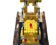
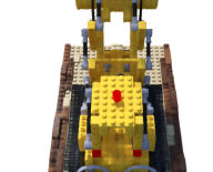
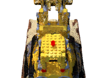
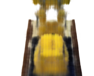
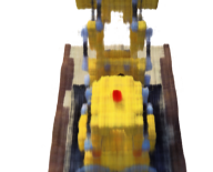
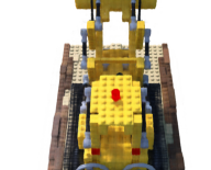
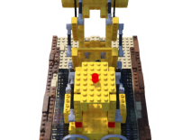
Visual Hull	0.5min	1min	5min	15min	30min

Figure 3: Top row is (Jax)NeRF (c64f128) results, bottom row is VaxNeRF (vax_c600) results. The elapsed time of VaxNeRF includes the time taken by Visual Hull. (Ten seconds, though.) Thanks to the visual hull, VaxNeRF is able to acquire the shape very fast. For example, VaxNeRF can already start learning the smallest holes in the caterpillar in 5 minutes, while the original NeRF can only do so after about 30 minutes. Please see Supplementary Materials for more visualizations, including zoomed comparisons along longer time scales. Note that, the colors (textures) shown in the “Visual Hull” are not used for VaxNeRF training.

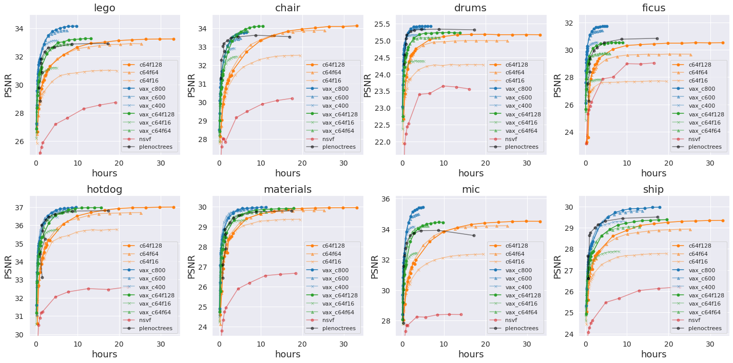
Figure 4: Comparison of training speed. Both VaxNeRF and NeRF trained 1 million iterations. The training of VaxNeRF was 2-8xtimes faster than the original NeRF, and furthermore, vax_c600 and vax_c800 had better accuracy than the original NeRF in most scenes. Note that PlenOctrees are converted to from the weights stored at some intervals during the training of NeRF-SH and then fine-tuned. Because the time required for fine tuning varies, the graph does not show a simple upward trend.

5.1 Experimental Setup

We detail the datasets and basic setups used in our experiments. More experimental setup details are included in Supplementary Materials.

Datasets

For our experiments, we use the NeRF-Synthetic dataset [41] and NSVF-Synthetic dataset [35]. The NeRF-Synthetic dataset and the NSVF-Synthetic dataset each consist of 8 scenes where each scene has a central object with 100 inward facing cameras distributed randomly on the upper hemisphere. All scenes exhibit complicated geometry and realistic non-Lambertian materials, but the NSVF-Synthetic dataset has more complex geometry, lighting effects and transparent parts, as shown in Figure 5. The images are 800 x 800 in resolution with ground-truth camera poses.

Baselines

The main baseline in our experiments is NeRF’s JAX re-implementation JaxNeRF [12]. It is slightly faster (much faster with parallel machines) to learn and inference, and easier to extend than the original implementation [41]. NeRF has a large number of fine sampling points by default (128) that may be unfair in speed comparisons, so we run it with different numbers of fine sampling points: 16, 64, and 128. In Figure 4 and Table 2, each NeRF result is denoted as cXfY using the number of coarse samples (X) and fine samples (Y). We also compare to two recent papers introducing NeRF accelerations: neural sparse voxel fields (NSVF) and PlenOctrees. Each experiment is run on a single NVIDIA A100 GPU.

VaxNeRF Implementation

Like NeRF, VaxNeRF is denoted as vax_cXfY using the number of coarse samples (X) and fine samples (Y) in Figure 4 and Table 2. Besides a modular visual hull function, we brought down the implementation to about 30 lines of change on top of JaxNeRF, as shown in Figure 2. Specifically, the only changes are to read in the voxels computed by our visual hull, add the voxels as an argument to the function, and then enter only the points inside the bounding volume into the MLP, and set values of zero for all other points. Unlike in NeRF where the number of points is fixed for all rays ($N$ in Eq. 1), in VaxNeRF it varies per ray due to rejecting points outside the bounding volume (Eq. 5). Since JAX does not efficiently handle variable-length inputs at the moment, in our current implementation we run the full NeRF model without rejection for 30 seconds, record the maximum number of points inside the volume across all rays, and compiles our code with the input sizes as “len_inpc” and “len_inpf” for coarse and (optional) fine models respectively.

Visual Hull Implementation

We use 400x400x400 resolution of voxels for visual hull. In addition, we need a binary mask separating the foreground from the background in each image. In the scenes where the alpha channel is given, we use it to directly derive the mask, but in some scenes of the NSVF-Synthetic dataset where it is not given, we use OpenCV to separate the background (white) from the foreground. In a real environment, one could use a green background, or apply an off-the-shelf segmentation model for separating objects of interest from the rest after capturing.

5.2 Experimental Results

We provide extensive evaluations on benchmark datasets against a series of strong baselines. More results are included in Supplementary Materials.

Qualitative Comparisons  In Figure 3, we show how NeRF and VaxNeRF visually compare in the first 30 minutes of training. We can observe substantial details emerge even with only 15-30 minutes of training on a single GPU. We also include the colored visualization of visual hull for reference, even though our method did not use this color information. This visual hull is optimized in the first 10 seconds, and yet it clearly captures intricate geometric details at 400x400x400 voxel resolution.

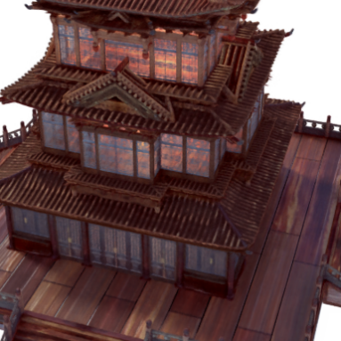
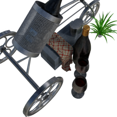
Figure 5: Qualitative results of VaxNeRF (vax_c600) on NSVF-Synthetic datasets, after 1 million training iterations, averaging 5.6 hours (this takes 33 hours on NeRF). VaxNeRF also performs well on objects with transparency and finer shapes.

Additionally, we show the final rendering quality of VaxNeRF on complex NSVF-Synthetic dataset [35]. As our quantitative metrics below and these visualizations illustrate, VaxNeRF does not degrade quality even on those scenes with complex geometry, lighting effects and transparent parts, unlike many other prior acceleration works in Table 1. This is because visual hull’s property and VaxNeRF’s design ensure that it converges to the same result as a full NeRF, as discussed in Section 4.1.

Quantitative Comparisons  Figure 4 plots PSNR over training time, where all results are performances on a single NVIDIA A100 GPU. We can cleanly observe that all VaxNeRF variants (“vax_X”) have fast convergence with high asymptotic accuracy. With sufficient point samples (vax_c600, vax_c800 and vax_c64f128), our VaxNeRF performs on par with NeRF in final rendering quality while speeding up the training by 2-8x, and sometimes even outperforms NeRF on final accuracy (vax_c600). Our results also compare favorably with results of NSVF and PlenOctrees reproduced from their official open-source implementations. NVSF, a popular model optimized for fast inference, appears slower in training since it gradually refines voxel resolutions during training. More surprisingly, compared to PlenOctrees which is substantially more complex and highly-optimized for both training and inference, VaxNeRF performs comparatively in terms of both speed and final rendering quality in all cases (except e.g. “ship”), slightly outperforming in PSNR and little under-performing in SSIM.  Table 2 summarizes these results comprehensively, where VaxNeRF, along with PlenOctrees, being the most performant across all time windows of training.

Method	number of samples	rays / sec
c64f128	802,816	34,424
c64f64	524,288	45,153
c64f16	327,680	58,610
vax_c64f128	363,625	89,151
vax_c64f64	211,625	141,086
vax_c64f16	97,875	240,489
vax_c800	184,500	148,812
vax_c600	138,500	192,489
vax_c400	92,125	275,824

Table 3: Training Speed Comparison on NeRF Synthesic Dataset. Measured on a single NVIDIA A100 GPU. Although vax_400, vax_600, and vax_800 sample the points on the ray quite finely in the voxel, the overall number of points to be sampled is dramatically reduced, and the training proceeds at a high ray/sec.

Notably, Figure 4 and Table 2 show that the most performant VaxNeRF only needs a single coarse model with dense point sampling (e.g. vax_600 and vax_800), a strong advantage of VaxNeRF over NeRF discussed in Section 4.1. Table 3 summarizes how our method dramatically reduces the number of points evaluated by NeRF, which in turn allows it to proceed with learning at a higher rays/sec. Our c_600 and c_800 VaxNeRF achieve training speed-ups of 5.35x and 4.11x per iteration respectively on average over a total of 16 scenes on the NeRF-Synthetic and NSVF-Synthetic datasets with little or no deterioration, or even slight improvements, in quality.

6 Discussion

While our empirical experiments conclusively demonstrate the speed-ups of VaxNeRF over NeRF, in this section we discuss possible explanations for such substantial gains, specifically:

• Effective Resolution for Point Selection: Both NeRF and VaxNeRF use heuristics to better allocate points for integral estimation along each ray (Eq. 1). Given that NeRF uses 64 samples for coarse model evaluations and VaxNeRF fits 400x400x400 visual hull, these correspond to effective resolutions of $1/64$ and $1/400$ respectively for selecting important regions along the ray. Despite NeRF using more direct estimate of contribution ($w_{i}$ instead of 0/1 masking) and visual hull’s imperfect boundary volume carving, this large effective resolution gap could explain VaxNeRF’s superior performance.

• Zero-Region Predictions: In NeRF, the 3D space regions where no object is present are constantly evaluated and optimized throughout the training for both coarse and fine models, while in VaxNeRF they are directly set to 0 without ever running MLP evaluations. This substantially could reduce the predictive burden on MLPs in VaxNeRF, leading to faster training.

We speculate that the overall speed-up arises from a combination of these design effects, and hope more future works probe into the fundamental building blocks of NeRF.

7 Conclusion

We present VaxNeRF, combining the classic visual hull technique with NeRF. Our implementation only takes about 30 lines of main code changes from JaxNeRF, and yet provides reliable 2-8x speed-ups compared to this strong baseline with no loss in rendering quality. We hope our results could encourage more works asking fundamental questions about algorithmic designs of the popular end-to-end methods, and revisiting classic approaches (that are supposedly replaced by these methods) within these methods.

Limitations and Future Work

The limitations of the current work are: (1) visual hull requires binary foreground-background masks, and (2) all results are on synthetic datasets. Evaluating VaxNeRF on real-world datasets are the next challenge, where we plan to curate and open-source such a dataset with ground-truth masks from green screen or an off-the-shelf segmentation model.

Appendix A Additional Experimental Setups

This table shows hyper-parameters we used for experiments. For NSVF and PlenOctrees, we ran the official implementation as is.

Method	batch_size	max_iteration	emb_dim
(Jax)NeRF	4,096	1,000,000	10
VaxNeRF	4,096	1,000,000	10
NSVF	4,096	150,000	10
PlenOctrees	1,024	2,000,000	10

Table 4: Hyper-parameters of each method.

Algorithm 1 NeRF and VaxNeRF (w/o hierarchical sampling). Added codes to NeRF and removed codes from NeRF

0:  dataset of rays and corresponding color $\mathcal{D}$

1:  while not done do

2:     Sample batch of rays and color $\{\{o_{i},d_{i}\},C_{i}\}\sim\mathcal{D}$

3:     Coarse sampling points along the ray $\mathbf{x}_{i}^{(c)}\Leftarrow\text{coarse\_sample}(o_{i},d_{i})$

4:     Evaluate color and density at each point $\mathbf{c}_{i}^{(c)},\mathbf{\sigma}_{i}^{(c)}=\text{MLP}_{\mathbf{\theta}_{c}}(\mathbf{x}_{i}^{(c)},d_{i})$

5:     Evaluate color and density at each point $\mathbf{c}_{i}^{(c)},\mathbf{\sigma}_{i}^{(c)}\Leftarrow\left\{\begin{matrix}\text{MLP}_{\mathbf{\theta}_{c}}(\mathbf{x}_{i}^{(c)},d_{i})\quad&(\mathbf{x}_{i}\in\mathcal{V})\\ \mathbf{0}\quad&(\mathbf{x}_{i}\notin\mathcal{V})\end{matrix}\right.$

6:     Compute pixel value using ray marching $\hat{C}_{i}^{(c)}\Leftarrow\text{ray\_marching}(\mathbf{x}_{i}^{(c)},\mathbf{c}_{i}^{(c)},\mathbf{\sigma}_{i}^{(c)})$

7:     fine sampling points along the ray $\mathbf{x}_{i}^{(f)}\Leftarrow\text{fine\_sample}(o_{i},d_{i})$

8:     Evaluate color and density at each point $\mathbf{c}_{i}^{(f)},\mathbf{\sigma}_{i}^{(f)}\Leftarrow\text{MLP}_{\mathbf{\theta}_{f}}(\mathbf{x}_{i}^{(f)},d_{i})$

9:     Compute pixel value using ray marching $\hat{C}_{i}^{(f)}\Leftarrow\text{ray\_marching}(\mathbf{x}_{i}^{(f)},\mathbf{c}_{i}^{(f)},\mathbf{\sigma}_{i}^{(f)})$

10:     Compute loss for each pixel $\mathcal{L}_{c}=\sum\big{\lVert}{C_{i}-\hat{C}_{i}^{(c)}}\big{\rVert}^{2}_{2}$, $\mathcal{L}_{f}=\sum\big{\lVert}{C_{i}-\hat{C}_{i}^{(f)}}\big{\rVert}^{2}_{2}$

11:     Update parameters $\mathbf{\theta}_{c}$, $\mathbf{\theta}_{f}$ using gradient descent

12:  end while

Appendix B Additional Experimental Results

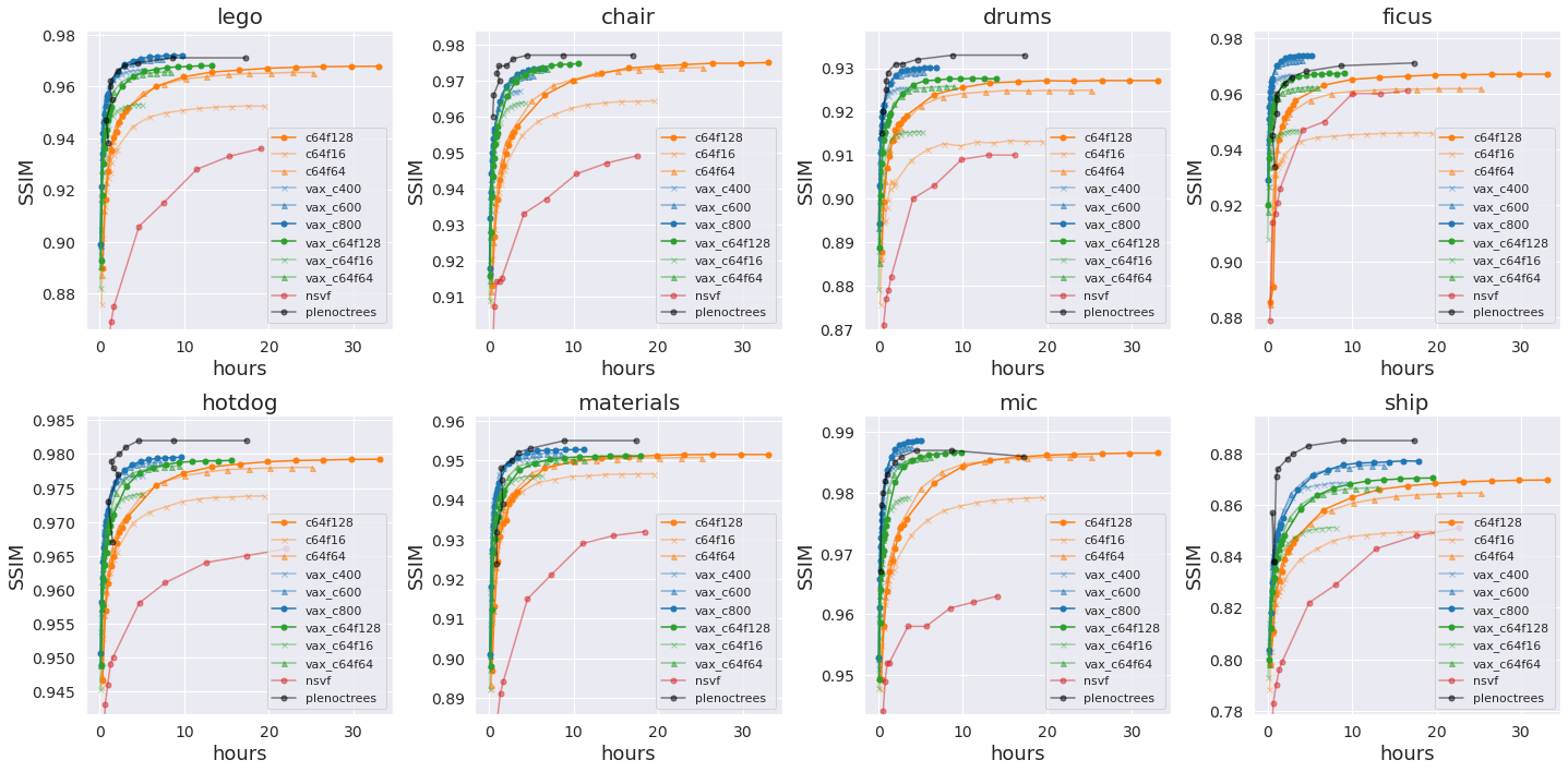
Figure 6: SSIM comparison on NeRF-Synthetic dataset

Synthetic NSVF Dataset     best second-best third-best
	0.5h		1h		3h		6h		12h		36h
Method	PSNR	SSIM	PSNR	SSIM	PSNR	SSIM	PSNR	SSIM	PSNR	SSIM	PSNR	SSIM
c64f64	28.05	0.922	29.32	0.936	31.03	0.952	32.06	0.959	32.74	0.964	32.98	0.965
c64f128	27.3	0.916	29.06	0.933	31.16	0.953	32.17	0.96	33.03	0.965	33.52	0.968
vax_c64f64	30.61	0.947	31.58	0.955	32.8	0.964	33.05	0.966	33.07	0.966	33.07	0.966
vax_c64f128	30.21	0.943	31.36	0.953	32.89	0.964	33.42	0.967	33.57	0.968	33.58	0.968
vax_c400	31.22	0.951	32.16	0.957	32.95	0.963	33.02	0.964	33.02	0.964	33.02	0.964
vax_c600	31.33	0.952	32.33	0.959	33.56	0.967	33.77	0.968	33.79	0.969	33.79	0.969
vax_c800	31.19	0.95	32.28	0.959	33.71	0.968	34.08	0.97	34.15	0.971	34.15	0.971
nsvf	26.68	0.902	28.41	0.923	29.82	0.939	31.03	0.952	31.92	0.962	32.68	0.97

Table 5: Quantitative results on NSVF-Synthetic dataset. Each value is the average of the eight scenes.

Figure 7: PSNR comparison on NSVF-Synthetic dataset

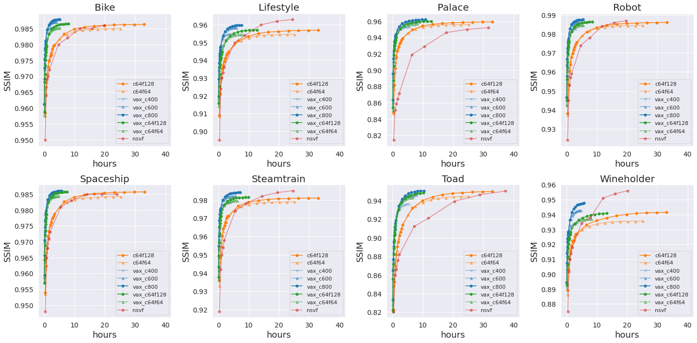
Figure 8: SSIM comparison on NSVF-Synthetic dataset

References

- [1] Michal Adamkiewicz, Timothy Chen, Adam Caccavale, Rachel Gardner, Preston Culbertson, Jeannette Bohg, and Mac Schwager. Vision-only robot navigation in a neural radiance world. arXiv preprint arXiv:2110.00168, 2021.
- [2] Alexander W. Bergman, Petr Kellnhofer, and Gordon Wetzstein. Fast training of neural lumigraph representations using meta learning. In NeurIPS, 2021.
- [3] Mark Boss, Raphael Braun, Varun Jampani, Jonathan T. Barron, Ce Liu, and Hendrik P.A. Lensch. Nerd: Neural reflectance decomposition from image collections. In IEEE International Conference on Computer Vision (ICCV), 2021.
- [4] Fabio Bruno, Stefano Bruno, Giovanna De Sensi, Maria-Laura Luchi, Stefania Mancuso, and Maurizio Muzzupappa. From 3d reconstruction to virtual reality: A complete methodology for digital archaeological exhibition. Journal of Cultural Heritage, 11(1):42–49, 2010.
- [5] Chris Buehler, Michael Bosse, Leonard McMillan, Steven Gortler, and Michael Cohen. Unstructured lumigraph rendering. SIGGRAPH, 2001.
- [6] Eric Chan, Marco Monteiro, Petr Kellnhofer, Jiajun Wu, and Gordon Wetzstein. pi-gan: Periodic implicit generative adversarial networks for 3d-aware image synthesis. In arXiv, 2020.
- [7] Anpei Chen, Zexiang Xu, Fuqiang Zhao, Xiaoshuai Zhang, Fanbo Xiang, Jingyi Yu, and Hao Su. Mvsnerf: Fast generalizable radiance field reconstruction from multi-view stereo. arXiv preprint arXiv:2103.15595, 2021.
- [8] Sun Cheng, Sun Min, and Chen Hwann-Tzong. Direct voxel grid optimization: Super-fast convergence for radiance fields reconstruction. arXiv preprint arXiv:2111.11215, 2021.
- [9] Abe Davis, Marc Levoy, and Fredo Durand. Unstructured light fields. In Computer Graphics Forum, volume 31, pages 305–314. Wiley Online Library, 2012.
- [10] Paul Debevec, C. J. Taylor, and Jitendra Malik. Modeling and rendering architecture from photographs: a hybrid geometry- and image-based approach. SIGGRAPH, 1992.
- [11] Frank Dellaert and Lin Yen-Chen. Neural volume rendering: Nerf and beyond. arXiv preprint arXiv:2101.05204, 2020.
- [12] Boyang Deng, Jonathan T. Barron, and Pratul P. Srinivasan. JaxNeRF: an efficient JAX implementation of NeRF, 2020.
- [13] Kangle Deng, Andrew Liu, Jun-Yan Zhu, and Deva Ramanan. Depth-supervised nerf: Fewer views and faster training for free. arXiv preprint arXiv:2107.02791, 2021.
- [14] SM Ali Eslami, Danilo Jimenez Rezende, Frederic Besse, Fabio Viola, Ari S Morcos, Marta Garnelo, Avraham Ruderman, Andrei A Rusu, Ivo Danihelka, Karol Gregor, et al. Neural scene representation and rendering. Science, 360(6394):1204–1210, 2018.
- [15] Simon Fuhrmann, Fabian Langguth, and Michael Goesele. Mve-a multi-view reconstruction environment. In GCH, pages 11–18. Citeseer, 2014.
- [16] Guy Gafni, Justus Thies, Michael Zollhöfer, and Matthias Nießner. Dynamic neural radiance fields for monocular 4d facial avatar reconstruction. In Proceedings of the IEEE/CVF Conference on Computer Vision and Pattern Recognition (CVPR), pages 8649–8658, June 2021.
- [17] Silvano Galliani, Katrin Lasinger, and Konrad Schindler. Massively parallel multiview stereopsis by surface normal diffusion. In Proceedings of the IEEE International Conference on Computer Vision, pages 873–881, 2015.
- [18] Stephan J Garbin, Marek Kowalski, Matthew Johnson, Jamie Shotton, and Julien Valentin. Fastnerf: High-fidelity neural rendering at 200fps. arXiv preprint arXiv:2103.10380, 2021.
- [19] Thomas Germer, Tobias Uelwer, Stefan Conrad, and Stefan Harmeling. Pymatting: A python library for alpha matting. Journal of Open Source Software, 5(54):2481, 2020.
- [20] Steven J Gortler, Radek Grzeszczuk, Richard Szeliski, and Michael F Cohen. The lumigraph. In Proceedings of the 23rd annual conference on Computer graphics and interactive techniques, pages 43–54, 1996.
- [21] Michelle Guo, Alireza Fathi, Jiajun Wu, and Thomas Funkhouser. Object-centric neural scene rendering. arXiv preprint arXiv:2012.08503, 2020.
- [22] Peter Hedman, Pratul P. Srinivasan, Ben Mildenhall, Jonathan T. Barron, and Paul Debevec. Baking neural radiance fields for real-time view synthesis. ICCV, 2021.
- [23] Michitaka Hirose. Virtual reality technology and museum exhibit. In International Conference on Virtual Storytelling, pages 3–11. Springer, 2005.
- [24] Yoonwoo Jeong, Seokjun Ahn, Christopher Choy, Anima Anandkumar, Minsu Cho, and Jaesik Park. Self-calibrating neural radiance fields. In Proceedings of the IEEE/CVF International Conference on Computer Vision, pages 5846–5854, 2021.
- [25] Abhishek Kar, Christian Häne, and Jitendra Malik. Learning a multi-view stereo machine. arXiv preprint arXiv:1708.05375, 2017.
- [26] Kiriakos N Kutulakos. Shape from the light field boundary. In Proceedings of IEEE Computer Society Conference on Computer Vision and Pattern Recognition, pages 53–59. IEEE, 1997.
- [27] Kiriakos N Kutulakos and Steven M Seitz. A theory of shape by space carving. International journal of computer vision, 38(3):199–218, 2000.
- [28] Aldo Laurentini. The visual hull concept for silhouette-based image understanding. IEEE Transactions on pattern analysis and machine intelligence, 16(2):150–162, 1994.
- [29] Marc Levoy and Pat Hanrahan. Light field rendering. In Proceedings of the 23rd annual conference on Computer graphics and interactive techniques, pages 31–42, 1996.
- [30] Yunzhu Li, Shuang Li, Vincent Sitzmann, Pulkit Agrawal, and Antonio Torralba. 3d neural scene representations for visuomotor control. arXiv preprint arXiv:2107.04004, 2021.
- [31] Zhengqi Li, Simon Niklaus, Noah Snavely, and Oliver Wang. Neural scene flow fields for space-time view synthesis of dynamic scenes. https://arxiv.org/abs/2011.13084, 2020.
- [32] Chen-Hsuan Lin, Wei-Chiu Ma, Antonio Torralba, and Simon Lucey. Barf: Bundle-adjusting neural radiance fields. In IEEE International Conference on Computer Vision (ICCV), 2021.
- [33] Shanchuan Lin, Andrey Ryabtsev, Soumyadip Sengupta, Brian Curless, Steve Seitz, and Ira Kemelmacher-Shlizerman. Real-time high-resolution background matting. arXiv, pages arXiv–2012, 2020.
- [34] D. B.* Lindell, J. N. P.* Martel, and G. Wetzstein. Autoint: Automatic integration for fast neural volume rendering. In Proc. CVPR, 2021.
- [35] Lingjie Liu, Jiatao Gu, Kyaw Zaw Lin, Tat-Seng Chua, and Christian Theobalt. Neural sparse voxel fields. NeurIPS, 2020.
- [36] Yuan Liu, Sida Peng, Lingjie Liu, Qianqian Wang, Peng Wang, Theobalt Christian, Xiaowei Zhou, and Wenping Wang. Neural rays for occlusion-aware image-based rendering. arXiv preprint arXiv:2107.13421, 2021.
- [37] Stephen Lombardi, Tomas Simon, Jason Saragih, Gabriel Schwartz, Andreas Lehrmann, and Yaser Sheikh. Neural volumes: Learning dynamic renderable volumes from images. ACM Trans. Graph., 38(4):65:1–65:14, July 2019.
- [38] Quan Meng, Anpei Chen, Haimin Luo, Minye Wu, Hao Su, Lan Xu, Xuming He, and Jingyi Yu. GNeRF: GAN-based Neural Radiance Field without Posed Camera. In Proceedings of the IEEE/CVF International Conference on Computer Vision (ICCV), 2021.
- [39] Michael Goesele Michael Waechter, Nils Moehrle. Let there be color! Large-scale texturing of 3D reconstructions. ECCV, 2014.
- [40] Ben Mildenhall, Pratul P. Srinivasan, Rodrigo Ortiz-Cayon, Nima Khademi Kalantari, Ravi Ramamoorthi, Ren Ng, and Abhishek Kar. Local light field fusion: Practical view synthesis with prescriptive sampling guidelines. ACM Transactions on Graphics (TOG), 2019.
- [41] Ben Mildenhall, Pratul P. Srinivasan, Matthew Tancik, Jonathan T. Barron, Ravi Ramamoorthi, and Ren Ng. Nerf: Representing scenes as neural radiance fields for view synthesis. In ECCV, 2020.
- [42] Anand Nayyar, Bandana Mahapatra, D Le, and G Suseendran. Virtual reality (vr) & augmented reality (ar) technologies for tourism and hospitality industry. International journal of engineering & technology, 7(2.21):156–160, 2018.
- [43] T. Neff, P. Stadlbauer, M. Parger, A. Kurz, J. H. Mueller, C. R. A. Chaitanya, A. Kaplanyan, and M. Steinberger. Donerf: Towards real-time rendering of compact neural radiance fields using depth oracle networks. Computer Graphics Forum, 40(4):45–59, 2021.
- [44] Thu Nguyen-Phuoc, Chuan Li, Lucas Theis, Christian Richardt, and Yong-Liang Yang. Hologan: Unsupervised learning of 3d representations from natural images. In The IEEE International Conference on Computer Vision (ICCV), Nov 2019.
- [45] Michael Niemeyer and Andreas Geiger. Giraffe: Representing scenes as compositional generative neural feature fields. In Proc. IEEE Conf. on Computer Vision and Pattern Recognition (CVPR), 2021.
- [46] Michael Niemeyer, Lars Mescheder, Michael Oechsle, and Andreas Geiger. Differentiable volumetric rendering: Learning implicit 3d representations without 3d supervision. In Proceedings of the IEEE/CVF Conference on Computer Vision and Pattern Recognition, pages 3504–3515, 2020.
- [47] Atsuhiro Noguchi, Xiao Sun, Stephen Lin, and Tatsuya Harada. Neural articulated radiance field. In International Conference on Computer Vision, 2021.
- [48] Michael Oechsle, Songyou Peng, and Andreas Geiger. Unisurf: Unifying neural implicit surfaces and radiance fields for multi-view reconstruction. In International Conference on Computer Vision (ICCV), 2021.
- [49] Julian Ost, Fahim Mannan, Nils Thuerey, Julian Knodt, and Felix Heide. Neural scene graphs for dynamic scenes. In Proceedings of the IEEE/CVF Conference on Computer Vision and Pattern Recognition (CVPR), pages 2856–2865, June 2021.
- [50] Keunhong Park, Utkarsh Sinha, Peter Hedman, Jonathan T. Barron, Sofien Bouaziz, Dan B Goldman, Ricardo Martin-Brualla, and Steven M. Seitz. Hypernerf: A higher-dimensional representation for topologically varying neural radiance fields. arXiv preprint arXiv:2106.13228, 2021.
- [51] Sida Peng, Junting Dong, Qianqian Wang, Shangzhan Zhang, Qing Shuai, Xiaowei Zhou, and Hujun Bao. Animatable neural radiance fields for modeling dynamic human bodies. In ICCV, 2021.
- [52] Martin Piala and Ronald Clark. Terminerf: Ray termination prediction for efficient neural rendering. arXiv preprint arXiv:2111.03643, 2021.
- [53] Daniel Rebain, Wei Jiang, Soroosh Yazdani, Ke Li, Kwang Moo Yi, and Andrea Tagliasacchi. Derf: Decomposed radiance fields. In Proceedings of the IEEE/CVF Conference on Computer Vision and Pattern Recognition, pages 14153–14161, 2021.
- [54] Christian Reiser, Songyou Peng, Yiyi Liao, and Andreas Geiger. Kilonerf: Speeding up neural radiance fields with thousands of tiny mlps. arXiv, 2021.
- [55] Johannes Lutz Schönberger and Jan-Michael Frahm. Structure-from-motion revisited. In Conference on Computer Vision and Pattern Recognition (CVPR), 2016.
- [56] Johannes Lutz Schönberger, Enliang Zheng, Marc Pollefeys, and Jan-Michael Frahm. Pixelwise view selection for unstructured multi-view stereo. In European Conference on Computer Vision (ECCV), 2016.
- [57] Katja Schwarz, Yiyi Liao, Michael Niemeyer, and Andreas Geiger. Graf: Generative radiance fields for 3d-aware image synthesis. In Advances in Neural Information Processing Systems (NeurIPS), 2020.
- [58] Steven M Seitz, Brian Curless, James Diebel, Daniel Scharstein, and Richard Szeliski. A comparison and evaluation of multi-view stereo reconstruction algorithms. In 2006 IEEE computer society conference on computer vision and pattern recognition (CVPR’06), volume 1, pages 519–528. IEEE, 2006.
- [59] Steven M Seitz and Charles R Dyer. Photorealistic scene reconstruction by voxel coloring. International Journal of Computer Vision, 35(2):151–173, 1999.
- [60] Ben Semerjian. A new variational framework for multiview surface reconstruction. In European Conference on Computer Vision, pages 719–734. Springer, 2014.
- [61] Pratul P. Srinivasan, Boyang Deng, Xiuming Zhang, Matthew Tancik, Ben Mildenhall, and Jonathan T. Barron. Nerv: Neural reflectance and visibility fields for relighting and view synthesis. In CVPR, 2021.
- [62] Edgar Sucar, Shikun Liu, Joseph Ortiz, and Andrew Davison. iMAP: Implicit mapping and positioning in real-time. In Proceedings of the International Conference on Computer Vision (ICCV), 2021.
- [63] Tiancheng Sun, Kai-En Lin, Sai Bi, Zexiang Xu, and Ravi Ramamoorthi. Nelf: Neural light-transport field for portrait view synthesis and relighting. In Eurographics Symposium on Rendering, 2021.
- [64] Yanan Sun, Chi-Keung Tang, and Yu-Wing Tai. Semantic image matting. In Proceedings of the IEEE Conference on Computer Vision and Pattern Recognition, 2021.
- [65] Richard Szeliski. Rapid octree construction from image sequences. CVGIP: Image understanding, 58(1):23–32, 1993.
- [66] Matthew Tancik, Ben Mildenhall, Terrance Wang, Divi Schmidt, Pratul P. Srinivasan, Jonathan T. Barron, and Ren Ng. Learned initializations for optimizing coordinate-based neural representations. In CVPR, 2021.
- [67] Edgar Tretschk, Ayush Tewari, Vladislav Golyanik, Michael Zollhöfer, Christoph Lassner, and Christian Theobalt. Non-rigid neural radiance fields: Reconstruction and novel view synthesis of a dynamic scene from monocular video. In IEEE International Conference on Computer Vision (ICCV). IEEE, 2021.
- [68] Alex Trevithick and Bo Yang. GRF: Learning a general radiance field for 3d scene representation and rendering. arXiv, 2021.
- [69] Richard Tucker and Noah Snavely. Single-view view synthesis with multiplane images. In The IEEE Conference on Computer Vision and Pattern Recognition (CVPR), June 2020.
- [70] Shubham Tulsiani, Tinghui Zhou, Alexei A Efros, and Jitendra Malik. Multi-view supervision for single-view reconstruction via differentiable ray consistency. In Proceedings of the IEEE conference on computer vision and pattern recognition, pages 2626–2634, 2017.
- [71] Jayaram K Udupa and Gabor T Herman. 3D imaging in medicine. CRC press, 1999.
- [72] Krzysztof Walczak, Wojciech Cellary, and Martin White. Virtual museum exbibitions. Computer, 39(3):93–95, 2006.
- [73] Peng Wang, Lingjie Liu, Yuan Liu, Christian Theobalt, Taku Komura, and Wenping Wang. Neus: Learning neural implicit surfaces by volume rendering for multi-view reconstruction. NeurIPS, 2021.
- [74] Qianqian Wang, Zhicheng Wang, Kyle Genova, Pratul Srinivasan, Howard Zhou, Jonathan T. Barron, Ricardo Martin-Brualla, Noah Snavely, and Thomas Funkhouser. Ibrnet: Learning multi-view image-based rendering. In CVPR, 2021.
- [75] ZiYun Wang, Liao Wang, Fuqiang Zhao, Minye Wu, Lan Xu, and Jingyi Yu. Mirrornerf: One-shot neural portrait radiance field from multi-mirror catadioptric imaging. 2021 IEEE International Conference on Computational Photography (ICCP), pages 1–12, 2021.
- [76] Matthew J Westoby, James Brasington, Niel F Glasser, Michael J Hambrey, and Jennifer M Reynolds. ‘structure-from-motion’photogrammetry: A low-cost, effective tool for geoscience applications. Geomorphology, 179:300–314, 2012.
- [77] Suttisak Wizadwongsa, Pakkapon Phongthawee, Jiraphon Yenphraphai, and Supasorn Suwajanakorn. Nex: Real-time view synthesis with neural basis expansion. In IEEE Conference on Computer Vision and Pattern Recognition (CVPR), 2021.
- [78] Daniel Wood, Daniel Azuma, Wyvern Aldinger, Brian Curless, Tom Duchamp, David Salesin, and Werner Stuetzle. Surface light fields for 3D photography. SIGGRAPH, 2000.
- [79] Bangbang Yang, Yinda Zhang, Yinghao Xu, Yijin Li, Han Zhou, Hujun Bao, Guofeng Zhang, and Zhaopeng Cui. Learning object-compositional neural radiance field for editable scene rendering. In International Conference on Computer Vision (ICCV), October 2021.
- [80] Lior Yariv, Jiatao Gu, Yoni Kasten, and Yaron Lipman. Volume rendering of neural implicit surfaces. CoRR, abs/2106.12052, 2021.
- [81] Lior Yariv, Jiatao Gu, Yoni Kasten, and Yaron Lipman. Volume rendering of neural implicit surfaces. CoRR, abs/2106.12052, 2021.
- [82] Lin Yen-Chen, Pete Florence, Jonathan T. Barron, Alberto Rodriguez, Phillip Isola, and Tsung-Yi Lin. iNeRF: Inverting neural radiance fields for pose estimation. In IEEE/RSJ International Conference on Intelligent Robots and Systems (IROS), 2021.
- [83] Wang Yifan, Shihao Wu, Cengiz Oztireli, and Olga Sorkine-Hornung. Iso-points: Optimizing neural implicit surfaces with hybrid representations. In CVPR, 2020.
- [84] Alex Yu, Ruilong Li, Matthew Tancik, Hao Li, Ren Ng, and Angjoo Kanazawa. PlenOctrees for real-time rendering of neural radiance fields. In ICCV, 2021.
- [85] Alex Yu, Vickie Ye, Matthew Tancik, and Angjoo Kanazawa. pixelNeRF: Neural radiance fields from one or few images. In CVPR, 2021.
- [86] Kai Zhang, Gernot Riegler, Noah Snavely, and Vladlen Koltun. Nerf++: Analyzing and improving neural radiance fields. arXiv:2010.07492, 2020.
- [87] Xiuming Zhang, Pratul P Srinivasan, Boyang Deng, Paul Debevec, William T Freeman, and Jonathan T Barron. NeRFactor: Neural Factorization of Shape and Reflectance Under an Unknown Illumination. arXiv preprint arXiv:2106.01970, 2021.
- [88] Tinghui Zhou, Richard Tucker, John Flynn, Graham Fyffe, and Noah Snavely. Stereo magnification: Learning view synthesis using multiplane images. arXiv preprint arXiv:1805.09817, 2018.