Block Coordinate Descent for smooth nonconvex constrained minimization ^,

Abstract

At each iteration of a Block Coordinate Descent method one minimizes an approximation of the objective function with respect to a generally small set of variables subject to constraints in which these variables are involved. The unconstrained case and the case in which the constraints are simple were analyzed in the recent literature. In this paper we address the problem in which block constraints are not simple and, moreover, the case in which they are not defined by global sets of equations and inequations. A general algorithm that minimizes quadratic models with quadratric regularization over blocks of variables is defined and convergence and complexity are proved. In particular, given tolerances $\delta>0$ and $\varepsilon>0$ for feasibility/complementarity and optimality, respectively, it is shown that a measure of $(\delta,0)$-criticality tends to zero; and the the number of iterations and functional evaluations required to achieve $(\delta,\varepsilon)$-criticality is $O(\varepsilon^{2})$. Numerical experiments in which the proposed method is used to solve a continuous version of the traveling salesman problem are presented.

Key words: Coordinate descent methods, convergence, complexity.

AMS subject classifications: 90C30, 65K05, 49M37, 90C60, 68Q25.

1 Introduction

The structure of many practical problems suggests the employment of Block Coordinate Descent (BCD) methods for Optimization. At each iteration of a BCD method only a block of variables is modified with the purpose of obtaining sufficient decrease of the objective function.

Wright [9] surveyed traditional approaches and modern advances on the definition and analysis of Coordinate Descent methods. His analysis addresses mostly unconstrained problems in which the objective function is convex. Although the Coordinate Descent paradigm is very natural and is implicitly used in different mathematical contexts, a classical example by Powell [8] showed that convergence results cannot be achieved under excessively naive implementations.

In a recent report [2] it was shown that, requiring sufficient descent based on regularization, the drawbacks represented by Powell’s example can be removed. In that paper it was also shown that methods based on high-order regularization can be defined in which convergence and worst-case complexity can be proved. However, the main results shown in [2] indicate that it is not worthwhile to use Taylor-like models of order greater than 2 because complexity is dominated by the necessity of keeping consecutive iterations close enough, a requirement that is hard to achieve if models and regularizations are of high order. This is the reason why, in the present paper, we restrict ourselves to quadratic models of the objective function and quadratic regularization.

The novelty of our approach relies in the employment of a general feasible set for each block of variables. As a consequence, at each iteration of BCD we minimize a problem with (probably) a small number of variables that must satisfy arbitrary constraints. Moreover, the block feasible set may not be defined by a global set of equalities and inequalities, as usually in constrained optimization. Instead, equalities and inequalities that define the feasible set are local in nature in a sense that will be defined below, making it possible more general domains than the ones defined by global equalities and inequalities.

This paper is organized as follows. In Section 2 the definition of the optimization problem is given. In Section 3 we define the BCD method for solving the main problem. In Section 4 we prove convergence and complexity results. In Section 5 we explain how to solve subproblems. Experiments are shown in Section 6 and in Section 7 we state conclusions and lines for future research.

Notation. $\|\cdot\|$ denotes the Euclidean norm. $\nabla_{i}$ denotes the gradient with respect to the $i$th block of coordinates. $\mathbb{N}=\{0,1,2,\ldots\}$.

2 The problem

Assume that $f:\mathbb{R}^{n}\to\mathbb{R}$, $n_{i}\geq 1$ for all $i=1,\ldots,n_{\mathrm{blocks}}$, and $\sum_{i=1}^{n_{\mathrm{blocks}}}n_{i}=n$. Let us write $x^{T}=(\boldsymbol{x}_{1}^{T},\dots,\boldsymbol{x}_{n_{\mathrm{blocks}}}^{T})^{T}$, where $\boldsymbol{x}_{i}\in\mathbb{R}^{n_{i}}$ for all $i=1,\dots,n_{\mathrm{blocks}}$, so

$$f(x)=f(x_{1},\dots,x_{n})=f(\boldsymbol{x}_{1},\dots,\boldsymbol{x}_{n_{\mathrm{blocks}}}).$$

The problem considered in the present work is given by

$$\operatorname*{Minimize}f(\boldsymbol{x}_{1},\dots,\boldsymbol{x}_{n_{\mathrm{blocks}}})\mbox{ subject to }\boldsymbol{x}_{i}\in\Omega_{i},i=1,\dots,n_{\mathrm{blocks}}.$$ (1)

The assumption below includes conditions on the sets $\Omega_{i}$ and on the way they are described.

Assumption A1

For all $i=1,\dots,n_{\mathrm{blocks}}$ the set $\Omega_{i}\subset\mathbb{R}^{n_{i}}$ is closed and bounded. Moreover, for all $i=1,\dots,n_{\mathrm{blocks}}$, there exist open sets $A_{i,j}$, $j=1,\dots,n_{\mathrm{ops}}(i)$, such that

$$\Omega_{i}\subset\cup_{j=1}^{n_{\mathrm{ops}}(i)}A_{i,j}$$

and there exist $n_{\mathrm{g}}(i,j)$ smooth functions

$$g_{i,j,\ell}:A_{i,j}\to\mathbb{R},\;\ell=1,\dots,n_{\mathrm{g}}(i,j)$$ (2)

such that

$$\Omega_{i}\cap A_{i,j}=\{\boldsymbol{x}_{i}\in A_{i,j}\;|\;g_{i,j,\ell}(\boldsymbol{x}_{i})\leq 0,\;\ell=1,\dots,n_{\mathrm{g}}(i,j)\}.$$ (3)

The constraints $g_{i,j,\ell}(\boldsymbol{x}_{i})\leq 0$ are said to be constitutive of $\Omega_{i}$ in the open covering set $A_{i,j}$. The explicit inclusion of equality constraints in (2,3) offers no difficulty and we state the case with only inequalities for the sole purpose of simplifying the notation. See Figure 1 for an example of a set $\Omega_{i}$, the open covering $A_{i,j}$ and functions $g_{i,j,\ell}$.

Figure 1: Illustration of a set $\Omega_{1}$ (dashed red) covered by $n_{\mathrm{ops}}(1)=12$ open sets $A_{1,1},\dots,A_{1,12}$.

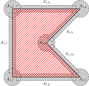
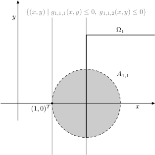
In Figure 1, sets $A_{1,j}$ for $j=1,2,3,5$ (four out of the five open circles) are such that $n_{g}(1,j)=2$; while sets $A_{1,j}$ for $j=6,7,8,9,10$ (the open rectangles) are such that $n_{g}(1,j)=1$. In all cases, constitutive constraints are linear. Sets $A_{1,11}$ and $A_{1,12}$ are not displayed in the picture for clarity. They are two congruent open triangles that cover the interior of $\Omega_{1}$ that appears unconvered in the picture; and they are such that $n_{g}(1,11)=n_{g}(1,12)=0$. The “internal kink” at $A_{1,4}$ makes the constitutive constraint of $A_{1,4}$ to deserve special consideration. In $A_{1,4}$ the feasible region is the complement of a set defined by constraints of the form $a_{1}x_{1}+b_{1}x_{2}+c_{1}\geq 0$ and $a_{2}x_{1}+b_{2}x_{2}+c_{2}\geq 0$. Let us write $z_{1}=a_{1}x_{1}+b_{1}x_{2}+c_{1}$ and $z_{2}=a_{2}x_{1}+b_{2}x_{2}+c_{2}$. Then, in the plane $(z_{1},z_{2})$ the feasible region is, locally, the complement of the non-negative orthant. Define $\varphi(z_{1},z_{2})=(z_{1}z_{2})^{2}$ if $z_{1}\geq 0$ and $z_{2}\geq 0$, whereas $\varphi(z_{1},z_{2})=-(z_{1}z_{2})^{2}$ otherwise. Then, the feasible region is, locally, given by $\varphi(z_{1},z_{2})\leq 0$; i.e. $n_{g}(1,4)=1$ and the constitutive constraint is given by $\varphi$.

For further reference (in Section 5), we show here that the center $C_{1,4}$ of the ball $A_{1,4}$ satisfies KKT conditions. Clearly, the origin in the plane $(z_{1},z_{2})$, which corresponds to the point $C_{1,4}$, is a non-regular point from the point of view of constrained optimization. However, if a smooth function $\psi$ has a minimizer at this point, its gradient $\nabla\psi(A_{1,4})$ is necessarily null. To see this observe that it is easy to show two linearly independent directions $v_{1}$ and $v_{2}$ such that $\nabla\psi(C_{1,4})^{T}v_{1}\geq 0$, $\nabla\psi(C_{1,4})^{T}(-v_{1})\geq 0$, $\nabla\psi(C_{1,4})^{T}v_{2}\geq 0$, and $\nabla\psi(C_{1,4})^{T}(-v_{2})\geq 0$, implying that $\nabla\psi(C_{1,4})=0$, so that $C_{1,4}$ is a KKT point of the minimization of $\psi$ subject to $\varphi\leq 0$ with a single null multiplier.

3 Block Coordinate Descent method

In this section we present the main algorithm designed for solving (1). At each iteration $k$ of the Block Coordinate Descent (BCD) method, given the current iterate $\boldsymbol{x}^{k}=((\boldsymbol{x}_{1}^{k})^{T},\dots,(\boldsymbol{x}_{n_{\mathrm{blocks}}}^{k})^{T})^{T}$, we choose $i_{k}\in\{1,\dots,n_{\mathrm{blocks}}\}$ and compute $\boldsymbol{x}_{i_{k}}^{k+1}$ by approximately solving

$$\operatorname*{Minimize}_{\boldsymbol{x}_{i_{k}}\in\mathbb{R}^{n_{i}}}f(\boldsymbol{x}_{1},\dots,\boldsymbol{x}_{n_{\mathrm{blocks}}})\mbox{ subject to }\boldsymbol{x}_{i_{k}}\in\Omega_{i_{k}}\mbox{ and }\boldsymbol{x}_{j}=\boldsymbol{x}_{j}^{k}\mbox{ for all }j\neq i_{k},$$ (4)

i.e. we approximately minimize the function $f$ fixing the blocks $\boldsymbol{x}_{j}$ such that $j\neq i_{k}$. For $j\neq i_{k}$, we define $\boldsymbol{x}_{j}^{k+1}=\boldsymbol{x}_{j}^{k}$. The sense in which problem (4) is solved only approximately is clarified below.

The algorithmic parameters of BCD are the sufficient descent parameter $\alpha$, which defines progress of the objective function and implicitly penalizes the distance between consecutive iterates, the tolerance $\delta$ with respect to complementarity conditions, the parameter $\theta$ that defines sufficient descent of the model at each iteration, and the minimal positive regularization parameter $\sigma_{\min}$. The model Hessian matrices $B_{k}$ may be used to mimic available second derivative information but do not play any significative role from the point of view of complexity or convergence and the choice $B_{k}=0$ is always possible. At Step 2 of the algorithm we choose the block of variables with respect to which we wish to improve the objective function. In general, we minimize approximately a quadratic model increasing the regularizing parameter as far as the suffcient condition (10) is not satisfied. Alternatively, we employ the true objective function as a model, because such alternative is possible in many practical problems.

Algorithm 3.1. Assume that $\alpha>0$, $\delta\geq 0$, $\theta>0$, $\sigma_{\min}>0$, and $\boldsymbol{x}_{i}^{0}\in\Omega_{i}$ for $i=1,\dots,n_{\mathrm{blocks}}$ are given. Initialize the iteration number $k\leftarrow 0$.

Step 1.

Set $\sigma\leftarrow 0$, choose $i_{k}\in\{1,\dots,n_{\mathrm{blocks}}\}$, and define $B_{k}\in\mathbb{R}^{n_{i_{k}}}\times\mathbb{R}^{n_{i_{k}}}$ symmetric.

Step 2.

Find $j_{k}\in\{1,\dots,n_{\mathrm{ops}}(i_{k})\}$ and $\boldsymbol{x}_{i_{k}}^{{\mathrm{trial}}}\in A_{i_{k},j_{k}}$ such that if $\sigma>0$ then Alternative 1 holds while if $\sigma=0$ then either Alternative 1 or Alternative 2 holds.

Alternative 1:

$$\nabla_{i_{k}}f(x^{k})^{T}(\boldsymbol{x}_{i_{k}}^{{\mathrm{trial}}}-\boldsymbol{x}_{i_{k}}^{k})+\frac{1}{2}(\boldsymbol{x}_{i_{k}}^{{\mathrm{trial}}}-\boldsymbol{x}_{i_{k}}^{k})^{T}B_{k}(\boldsymbol{x}_{i_{k}}^{{\mathrm{trial}}}-\boldsymbol{x}_{i_{k}}^{k})+\frac{\sigma}{2}\|\boldsymbol{x}_{i_{k}}^{{\mathrm{trial}}}-\boldsymbol{x}_{i_{k}}^{k}\|^{2}\leq 0$$ (5)

and there exist $\mu_{i_{k},j_{k},\ell}\geq 0$ for $\ell=1,\dots,n_{\mathrm{g}}(i_{k},j_{k})$ for which

$$\left\|\nabla_{i_{k}}f(x^{k})+B_{k}(\boldsymbol{x}_{i_{k}}^{{\mathrm{trial}}}-\boldsymbol{x}_{i_{k}}^{k})+\sigma(\boldsymbol{x}_{i_{k}}^{{\mathrm{trial}}}-\boldsymbol{x}_{i_{k}}^{k})+\sum_{\ell=1}^{n_{\mathrm{g}}(i_{k},j_{k})}\mu_{i_{k},j_{k},\ell}\nabla g_{i_{k},j_{k},\ell}(\boldsymbol{x}_{i_{k}}^{{\mathrm{trial}}})\right\|\leq\theta\|\boldsymbol{x}_{i_{k}}^{{\mathrm{trial}}}-\boldsymbol{x}_{i_{k}}^{k}\|$$ (6)

and

$$\min\{\mu_{i_{k},j_{k},\ell},-g_{i_{k},j_{k},\ell}(\boldsymbol{x}_{i_{k}}^{{\mathrm{trial}}})\}\leq\delta,\;\ell=1,\dots,n_{\mathrm{g}}(i_{k},j_{k}).$$ (7)

Alternative 2:

There exist $\mu_{i_{k},j_{k},\ell}\geq 0$ for $\ell=1,\dots,n_{\mathrm{g}}(i_{k},j_{k})$ for which

$$\left\|\nabla_{i_{k}}f(\boldsymbol{x}_{1}^{k},\dots,\boldsymbol{x}_{i_{k}}^{{\mathrm{trial}}},\dots,\boldsymbol{x}_{n_{\mathrm{blocks}}}^{k})+\sum_{\ell=1}^{n_{\mathrm{g}}(i_{k},j_{k})}\mu_{i_{k},j_{k},\ell}\nabla g_{i_{k},j_{k},\ell}(\boldsymbol{x}_{i_{k}}^{{\mathrm{trial}}})\right\|=0$$ (8)

and

$$\min\{\mu_{i_{k},j_{k},\ell},-g_{i_{k},j_{k},\ell}(\boldsymbol{x}_{i_{k}}^{{\mathrm{trial}}})\}\leq 0,\;\ell=1,\dots,n_{\mathrm{g}}(i_{k},j_{k}).$$ (9)

Step 3.

Test the sufficient descent condition

$$f(\boldsymbol{x}_{1}^{k},\dots,\boldsymbol{x}_{i_{k}}^{{\mathrm{trial}}},\dots,\boldsymbol{x}_{n_{\mathrm{blocks}}}^{k})\leq f(x^{k})-\alpha\|\boldsymbol{x}_{i_{k}}^{{\mathrm{trial}}}-\boldsymbol{x}_{i_{k}}^{k}\|^{2}.$$ (10)

If (10) holds, then define $\sigma_{k}=\sigma$, $x_{i_{k}}^{k+1}=x_{i_{k}}^{{\mathrm{trial}}}$ and $x_{i}^{k+1}=x_{i}^{k}$ for all $i\neq i_{k}$, set $k\leftarrow k+1$ and go to Step 1. Otherwise, set $\sigma\leftarrow\max\{\sigma_{\min},2\sigma\}$ and go to Step 2.

Remark. We will see that, from the theoretical point of view, Alternative 2 is not necessary. Convergence and complexity theoretical results follow without any difficulty with Alternative 1 only. Alternative 2 was included because, in many cases, a procedure exists to find a global minimizer with respect to a single block. So, in Alternative 2 we allow the algorithm to choose such minimizer, with the only condition that it must satisfy KKT conditions in the block. However, note that the test (10) is still necessary and cannot be eliminated. The reason is that its fulfillment implies that the difference between consecutive iterations tends to zero and this feature is essential for the convergence of coordinate search methods. See the counterexample in [8] and the discussion with only box constraints in [2].

4 Convergence and complexity

In this section we prove convergence and complexity results. We say that $(\boldsymbol{x}_{1},\dots,\boldsymbol{x}_{n_{\mathrm{blocks}}})$ is $(\delta,\varepsilon)$-critical if there exist open sets $A_{i,j}$ ($i=1,\dots,n_{\mathrm{blocks}}$, $j=1,\dots,n_{\mathrm{ops}}(i)$) satisfying Assumption A1 such that, for all $i=1,\dots,n_{\mathrm{blocks}}$, $\boldsymbol{x}_{i}$ satisfies the KKT conditions for the minimization of $f(\boldsymbol{x}_{1},\ldots,\boldsymbol{x}_{n_{\mathrm{blocks}}})$ restricted to the constitutive constraints of $A_{i,j}$, $j=1\dots,n_{\mathrm{ops}}(i)$, with tolerance $\varepsilon>0$ and satisfies complementarity and feasibility with respect to the same constraints with tolerance $\delta>0$. Under proper assumptions we prove that, given $\delta\geq 0$ (which is a parameter of the algorithm BCD), the natural measure of $(\delta,0)$-criticality tends to zero and the number of iterations and evaluations that are necessary to obtain $(\delta,\varepsilon)$-criticality is $O(\varepsilon^{2})$.

In Assumption A2 we state that the gradients of the objective function must satisfy Lipschitz conditions.

Assumption A2

There exists $\gamma>0$ such that, for all $\boldsymbol{x}_{i_{k}}$ and $\boldsymbol{x}_{i_{k}}^{{\mathrm{trial}}}$ computed at Algorithm 3.1,

$$\|\nabla_{i_{k}}f(x^{k})-\nabla_{i_{k}}f(\boldsymbol{x}_{1}^{k},\dots,\boldsymbol{x}_{i_{k}}^{{\mathrm{trial}}},\dots,\boldsymbol{x}_{n_{\mathrm{blocks}}}^{k})\|\leq\gamma\|\boldsymbol{x}_{i_{k}}-\boldsymbol{x}_{i_{k}}^{{\mathrm{trial}}}\|$$ (11)

and

$$f(\boldsymbol{x}_{1}^{k},\dots,\boldsymbol{x}_{i_{k}}^{{\mathrm{trial}}},\dots,\boldsymbol{x}_{n_{\mathrm{blocks}}}^{k})\leq f(x^{k})+\nabla_{i_{k}}f(x^{k})^{T}(\boldsymbol{x}_{i_{k}}^{{\mathrm{trial}}}-\boldsymbol{x}_{i_{k}}^{k})+\frac{\gamma}{2}\|\boldsymbol{x}_{i_{k}}-\boldsymbol{x}_{i_{k}}^{{\mathrm{trial}}}\|^{2}.$$ (12)

Moreover, if $x^{k_{1}}$ differs from $x^{k_{2}}$ in only one block $i_{\mathrm{diff}}$,

$$\|\nabla_{i}f(x^{k_{1}})-\nabla_{i}f(x^{k_{2}})\|\leq\gamma\|\boldsymbol{x}_{i_{\mathrm{diff}}}^{k_{2}}-\boldsymbol{x}_{i_{\mathrm{diff}}}^{k_{1}}\|.$$ (13)

for all $i=1,\dots,n_{\mathrm{blocks}}$.

Assumption A3 merely states that model Hessians should be uniformly bounded.

Assumption A3

There exist $c_{B}>0$ such that for all $k\in\mathbb{N}$,

$$\|B_{k}\|\leq c_{B}.$$ (14)

Assumptions A2 and A3 are sufficient to prove that every iteration of BCD is well defined, as sufficient descent (10) is obtained increasing the regularization parameter $\sigma$ a finite number of times.

Lemma 4.1

Assume that Assumptions A2 and A3 hold and that, for all $k\in\mathbb{N}$, the computation of $j_{k}$ and $\boldsymbol{x}_{i_{k}}^{{\mathrm{trial}}}$ according to Step 2 of BCD is possible. Then, the test (10) is satisfied after at most

$$\log_{2}\left(\frac{\gamma+c_{B}+2\alpha}{\sigma_{\min}}\right)+1$$

increases of $\sigma$ at Step 3. Moreover,

$$\sigma_{k}<\sigma_{\max}:=2(\gamma+c_{B}+2\alpha).$$ (15)

Proof: If the test (10) is satisfied when Step 2 is executed with $\sigma=0$, then the thesis holds trivially. So, we need to consider only the case in which $\sigma>0$ and, in consequence, $j_{k}$ and $\boldsymbol{x}_{i_{k}}^{{\mathrm{trial}}}$ satisfy Alternative 1. By (12) in Assumption A2,

$$f(\boldsymbol{x}_{1}^{k},\dots,\boldsymbol{x}_{i_{k}}^{{\mathrm{trial}}},\dots,\boldsymbol{x}_{n_{\mathrm{blocks}}}^{k}) \leq f(x^{k})+\nabla_{i_{k}}f(x^{k})^{T}(\boldsymbol{x}_{i_{k}}^{{\mathrm{trial}}}-\boldsymbol{x}_{i_{k}}^{k})+\frac{\gamma}{2}\|\boldsymbol{x}_{i_{k}}-\boldsymbol{x}_{i_{k}}^{{\mathrm{trial}}}\|^{2}$$

$$+\left(\frac{1}{2}(\boldsymbol{x}_{i_{k}}^{{\mathrm{trial}}}-\boldsymbol{x}_{i_{k}}^{k})^{T}B_{k}(\boldsymbol{x}_{i_{k}}^{{\mathrm{trial}}}-\boldsymbol{x}_{i_{k}}^{k})+\frac{1}{2}\sigma\|\boldsymbol{x}_{i_{k}}^{{\mathrm{trial}}}-\boldsymbol{x}_{i_{k}}^{k}\|^{2}\right)$$

$$-\left(\frac{1}{2}(\boldsymbol{x}_{i_{k}}^{{\mathrm{trial}}}-\boldsymbol{x}_{i_{k}}^{k})^{T}B_{k}(\boldsymbol{x}_{i_{k}}^{{\mathrm{trial}}}-\boldsymbol{x}_{i_{k}}^{k})+\frac{1}{2}\sigma\|\boldsymbol{x}_{i_{k}}^{{\mathrm{trial}}}-\boldsymbol{x}_{i_{k}}^{k}\|^{2}\right)$$

Then, by (5),

$$f(\boldsymbol{x}_{1}^{k},\dots,\boldsymbol{x}_{i_{k}}^{{\mathrm{trial}}},\dots,\boldsymbol{x}_{n_{\mathrm{blocks}}}^{k})\leq f(x^{k})+\frac{\gamma}{2}\|\boldsymbol{x}_{i_{k}}-\boldsymbol{x}_{i_{k}}^{{\mathrm{trial}}}\|^{2}-\frac{1}{2}(\boldsymbol{x}_{i_{k}}^{{\mathrm{trial}}}-\boldsymbol{x}_{i_{k}}^{k})^{T}B_{k}(\boldsymbol{x}_{i_{k}}^{{\mathrm{trial}}}-\boldsymbol{x}_{i_{k}}^{k})-\frac{1}{2}\sigma\|\boldsymbol{x}_{i_{k}}^{{\mathrm{trial}}}-\boldsymbol{x}_{i_{k}}^{k}\|^{2}.$$

Therefore, by (14) in Assumption A3,

$$f(\boldsymbol{x}_{1}^{k},\dots,\boldsymbol{x}_{i_{k}}^{{\mathrm{trial}}},\dots,\boldsymbol{x}_{n_{\mathrm{blocks}}}^{k}) \leq f(x^{k})+\frac{\gamma}{2}\|\boldsymbol{x}_{i_{k}}-\boldsymbol{x}_{i_{k}}^{{\mathrm{trial}}}\|^{2}+\frac{1}{2}c_{B}\|\boldsymbol{x}_{i_{k}}^{{\mathrm{trial}}}-\boldsymbol{x}_{i_{k}}^{k}\|^{2}-\frac{1}{2}\sigma\|\boldsymbol{x}_{i_{k}}^{{\mathrm{trial}}}-\boldsymbol{x}_{i_{k}}^{k}\|^{2}$$

$$=f(x^{k})+\frac{1}{2}(\gamma+c_{B}-\sigma)\|\boldsymbol{x}_{i_{k}}^{{\mathrm{trial}}}-\boldsymbol{x}_{i_{k}}^{k}\|^{2}.$$

Then, the inequality (10) holds if

$$\frac{1}{2}(\gamma+c_{B}-\sigma)\|\boldsymbol{x}_{i_{k}}^{{\mathrm{trial}}}-\boldsymbol{x}_{i_{k}}^{k}\|^{2}\leq-\alpha\|\boldsymbol{x}_{i_{k}}^{{\mathrm{trial}}}-\boldsymbol{x}_{i_{k}}^{k}\|^{2},$$

i.e. if $\sigma\geq\gamma+c_{B}+2\alpha$. Since, by definition, $\sigma$ initially receives the value zero and then receives values of the form $2^{\ell-1}\sigma_{\min}$, where $\ell$ is the number of executions of $\sigma\leftarrow\max\{\sigma_{\min},2\sigma\}$, then the number of increases of $\sigma$ that are necessary to obtain (10) is bounded above by

$$\log_{2}\left(\frac{\gamma+c_{B}+2\alpha}{\sigma_{\min}}\right)+1$$

as we wanted to prove. Finally, (15) comes from the fact that the largest unsuccessful value of $\sigma$ must be strictly less than $\gamma+c_{B}+2\alpha$ and the next (successful) value is twice that amount by definition. $\Box$

Assumption A4

The sequence $\{f(\boldsymbol{x}^{k})\}$ is bounded below.

The following lemma is a simple consequence of (10) and Assumption A4.

Lemma 4.2

Assume that Assumptions A2, A3, and A4 hold and that for all $k\in\mathbb{N}$, the computation of $j_{k}$ and $\boldsymbol{x}_{i_{k}}^{{\mathrm{trial}}}$ at Step 2 is possible. Then, $\lim_{k\to\infty}\|\boldsymbol{x}_{i_{k}}^{k+1}-\boldsymbol{x}_{i_{k}}^{k}\|=\lim_{k\to\infty}\|\boldsymbol{x}^{k+1}-\boldsymbol{x}^{k}\|=0$ and, given $\varepsilon>0$, the number of iterations at which $\|\boldsymbol{x}_{i_{k}}^{k+1}-\boldsymbol{x}_{i_{k}}^{k}\|>\varepsilon$ is bounded above by

$$\frac{f(\boldsymbol{x}^{0})-f_{{\mathrm{bound}}}}{\alpha\varepsilon^{2}}$$ (16)

where $f_{{\mathrm{bound}}}$ is an arbitrary lower bound of $\{f(\boldsymbol{x}^{k})\}$.

Proof: By Assumption A4 there exists $f_{{\mathrm{bound}}}\in\mathbb{R}$ such that $f(\boldsymbol{x}^{k})\geq f_{{\mathrm{bound}}}$ for all $k\in\mathbb{N}$. Then, the fact that $\|\boldsymbol{x}^{k+1}_{i_{k}}-\boldsymbol{x}^{k}_{i_{k}}\|$ tends to zero comes from (10); and this implies that $\|\boldsymbol{x}^{k+1}-\boldsymbol{x}^{k}\|$ tends to zero as well because, by definition, $\|\boldsymbol{x}^{k+1}-\boldsymbol{x}^{k}\|=\|\boldsymbol{x}^{k+1}_{i_{k}}-\boldsymbol{x}^{k}_{i_{k}}\|$. Finally, if $\|\boldsymbol{x}_{i_{k}}^{k+1}-\boldsymbol{x}_{i_{k}}^{k}\|>\varepsilon$, then, by (10), $f(x^{k+1})\leq f(x^{k})-\alpha\varepsilon^{2}$; and this reduction can no occur more than (16) times, as we wanted to prove. $\Box$

Assumption A5 states that every block of components $i$ is chosen for minimization at infinitely many iterations and, moreover, at every $m$ consecutive iterations we necessarily find at least one at which $i$ is chosen.

Assumption A5

There exists $m\in\{1,2,\dots\}$ such that, for all $\nu\in\{1,\dots,n_{\mathrm{blocks}}\}$, $i_{k}=\nu$ infinitely many times and, if $k_{1}<k_{2}<k_{3},\dots$ is the set of all the iteration indices $k$ such that $i_{k}=\nu$, one has that $k_{1}\leq m$, and $k_{j+1}-k_{j}\leq m$ for all $j=1,2,3,\dots$.

The following theorems are the main convergence result of this paper. The idea is the following. According to Algorithm 3.1, at iteration $k$, we select a block $i_{k}=i_{{\mathrm{chosen}}}$ and optimize with respect to the variables of this block up to the approximate fulfillment of restricted KKT conditions. These restricted KKT conditions hold in one of the open sets that cover $\Omega_{i_{{\mathrm{chosen}}}}$ and involve the constraints that are constitutive in this open set. The variables $\boldsymbol{x}_{i_{{\mathrm{chosen}}}}$ do not change during some (less than $m$) iterations; therefore, during these iterations, thanks to the Lipschitz assumption (13), the approximate KKT conditions with respect to the variables $i_{{\mathrm{chosen}}}$ still hold with respect to the same open set and the same constitutive constraints used at iteration $k$. After these (less than $m$) iterations the block $i_{{\mathrm{chosen}}}$ is selected again, and the process is repeated. Since all the blocks are chosen infinitely many times in the way described by Assumption A5, approximate KKT conditions eventually hold with respect to all the blocks and we are able to establish the number of iterations that we need for the fulfillment of KKT conditions up to an arbitrary precision $\varepsilon$.

Theorem 4.1

Assume that Assumptions A2, A3, A4, and A5 hold and that for all $k\in\mathbb{N}$, the computation of $j_{k}$ and $\boldsymbol{x}_{i_{k}}^{{\mathrm{trial}}}$ at Step 2 is possible. For $i\in\{1,\dots,n_{\mathrm{blocks}}\}$ and $k\geq m$, define $o(i,k):=j_{\hat{k}}$, where $\hat{k}$ is the latest iteration (not larger than $k$) at which $i_{\hat{k}}=i$. Then, for $i\in\{1,\dots,n_{\mathrm{blocks}}\}$ and $k\geq m$, we have that $\mu_{i,o(i,k),\ell}\geq 0$ for $\ell=1,\dots,n_{\mathrm{g}}(i,o(i,k))$,

$$\boldsymbol{x}^{k}_{i}\in A_{i,o(i,k)},$$

$$\min\{\mu_{i,o(i,k),\ell},-g_{i,o(i,k),\ell}(\boldsymbol{x}^{k}_{i})\}\leq\delta,$$

and

$$\lim_{k\to\infty}\left\|\nabla_{i}f(x^{k})+\sum_{\ell=1}^{n_{\mathrm{g}}(i,o(i,k))}\mu_{i,o(i,k),\ell}\nabla g_{i,o(i,k),\ell}(\boldsymbol{x}^{k}_{i})\right\|=0.$$

Moreover, given $\varepsilon>0$, the number of iterations at which

$$\left\|\nabla_{i}f(x^{k})+\sum_{\ell=1}^{n_{\mathrm{g}}(i,o(i,k))}\mu_{i,o(i,k),\ell}\nabla g_{i,o(i,k),\ell}(\boldsymbol{x}^{k}_{i})\right\|>\varepsilon$$

is bounded above by

$$\frac{f(\boldsymbol{x}^{0})-f_{{\mathrm{bound}}}}{\alpha(\varepsilon/(c_{4}m))^{2}},$$

where $f_{{\mathrm{bound}}}$ is an arbitrary lower bound of $\{f(\boldsymbol{x}^{k})\}$ and

$$c_{4}:=c_{B}+\sigma_{\max}+\theta+\gamma.$$ (17)

Proof: Let $i\in\{1,\dots,n_{\mathrm{blocks}}\}$ be arbitrary. By Assumption A5, there exists $k_{1}\leq m$ such that $i_{k_{1}}=i$. Without loss of generality, in order to simplify the notation, suppose that $k_{1}=0$. Consider first the case where, in Step 2, Alternative 1 holds. Then, at iteration $k_{1}=0$ one defines $B_{0}$ and finds $j_{0}$, $\boldsymbol{x}_{i}^{1}\in A_{i,j_{0}}$, and $\mu_{i,j_{0},\ell}\geq 0$ for $\ell=1,\dots,n_{\mathrm{g}}(i,j_{0})$ such that

$$\left\|\nabla_{i}f(x^{0})+B_{0}(\boldsymbol{x}_{i}^{1}-\boldsymbol{x}_{i}^{0})+\sigma_{0}(\boldsymbol{x}_{i}^{1}-\boldsymbol{x}_{i}^{0})+\sum_{\ell=1}^{n_{\mathrm{g}}(i,j_{0})}\mu_{i,j_{0},\ell}\nabla g_{i,j_{0},\ell}(\boldsymbol{x}_{i}^{1})\right\|\leq\theta\|\boldsymbol{x}_{i}^{1}-\boldsymbol{x}_{i}^{0}\|$$ (18)

and

$$\min\{\mu_{i,j_{0},\ell},-g_{i,j_{0},\ell}(\boldsymbol{x}_{i}^{1})\}\leq\delta\;\mbox{ for }\;\ell=1,\dots,n_{\mathrm{g}}(i,j_{0}).$$ (19)

By (18) and (15),

$$\left\|\nabla_{i}f(x^{0})+\sum_{\ell=1}^{n_{\mathrm{g}}(i,j_{0})}\mu_{i,j_{0},\ell}\nabla g_{i,j_{0},\ell}(\boldsymbol{x}_{i}^{1})\right\|\leq(c_{B}+\sigma_{\max}+\theta)\|\boldsymbol{x}_{i}^{1}-\boldsymbol{x}_{i}^{0}\|.$$ (20)

Then, by (11),

$$\left\|\nabla_{i}f(\boldsymbol{x}_{1}^{0},\dots,\boldsymbol{x}_{i}^{1},\dots,\boldsymbol{x}_{n_{\mathrm{blocks}}}^{0})+\sum_{\ell=1}^{n_{\mathrm{g}}(i,j_{0})}\mu_{i,j_{0},\ell}\nabla g_{i,j_{0},\ell}(\boldsymbol{x}_{i}^{1})\right\|\leq(c_{B}+\sigma_{\max}+\theta+\gamma)\|\boldsymbol{x}_{i}^{1}-\boldsymbol{x}_{i}^{0}\|.$$ (21)

Since $\boldsymbol{x}_{s}^{1}=\boldsymbol{x}_{s}^{0}$ for every $s=1,\dots,n_{\mathrm{blocks}}$, $s\neq i$, by (21) and the definition of $c_{4}$ in (17), we have that

$$\left\|\nabla_{i}f(x^{1})+\sum_{\ell=1}^{n_{\mathrm{g}}(i,j_{0})}\mu_{i,j_{0},\ell}\nabla g_{i,j_{0},\ell}(\boldsymbol{x}_{i}^{1})\right\|\leq c_{4}\|\boldsymbol{x}_{i}^{1}-\boldsymbol{x}_{i}^{0}\|.$$ (22)

Recall that (19) and (22) were obtained under Alternative 1. On the other hand, under Alternative 2, (19) and (22) follow trivially from (9) and (8), respectively.

Since $\boldsymbol{x}^{2}$ may differ from $\boldsymbol{x}^{1}$ only in the block $i_{1}$, by (13), we have that

$$\|\nabla_{i}f(\boldsymbol{x}^{2})-\nabla_{i}f(\boldsymbol{x}^{1})\|\leq\gamma\|\boldsymbol{x}_{i_{1}}^{2}-\boldsymbol{x}_{i_{1}}^{1}\|.$$

Then, by (22),

$$\left\|\nabla_{i}f(x^{2})+\sum_{\ell=1}^{n_{\mathrm{g}}(i,j_{0})}\mu_{i,j_{0},\ell}\nabla g_{i,j_{0},\ell}(\boldsymbol{x}_{i}^{1})\right\|\leq c_{4}\|\boldsymbol{x}_{i}^{1}-\boldsymbol{x}_{i}^{0}\|+\gamma\|\boldsymbol{x}_{i_{1}}^{2}-\boldsymbol{x}_{i_{1}}^{1}\|.$$ (23)

Since $\boldsymbol{x}^{3}$ may differ from $\boldsymbol{x}^{2}$ only in the block $i_{2}$, by (13) and (23), we have that

$$\left\|\nabla_{i}f(x^{3})+\sum_{\ell=1}^{n_{\mathrm{g}}(i,j_{0})}\mu_{i,j_{0},\ell}\nabla g_{i,j_{0},\ell}(\boldsymbol{x}_{i}^{1})\right\|\leq c_{4}\|\boldsymbol{x}_{i}^{1}-\boldsymbol{x}_{i}^{0}\|+\gamma\|\boldsymbol{x}_{i_{1}}^{2}-\boldsymbol{x}_{i_{1}}^{1}\|+\gamma\|\boldsymbol{x}_{i_{2}}^{3}-\boldsymbol{x}_{i_{2}}^{2}\|.$$ (24)

So, using an inductive argument, for all $k\in\mathbb{N}$,

$$\left\|\nabla_{i}f(x^{k})+\sum_{\ell=1}^{n_{\mathrm{g}}(i,j_{0})}\mu_{i,j_{0},\ell}\nabla g_{i,j_{0},\ell}(\boldsymbol{x}_{i}^{1})\right\|\leq c_{4}\|\boldsymbol{x}_{i}^{1}-\boldsymbol{x}_{i}^{0}\|+\gamma\sum_{\nu=2}^{k}\|\boldsymbol{x}^{\nu}-\boldsymbol{x}^{\nu-1}\|.$$ (25)

Thus, by the definition of $c_{4}$ in (17), for all $k\in\mathbb{N}$,

$$\left\|\nabla_{i}f(x^{k})+\sum_{\ell=1}^{n_{\mathrm{g}}(i,j_{0})}\mu_{i,j_{0},\ell}\nabla g_{i,j_{0},\ell}(\boldsymbol{x}_{i}^{1})\right\|\leq c_{4}\sum_{\nu=1}^{k}\|\boldsymbol{x}^{\nu}-\boldsymbol{x}^{\nu-1}\|.$$ (26)

Let us now get rid of the simplifying assumption $i_{0}=i$ and assume that the set of indices $k$ at which $i_{k}=i$ is $k_{1}<k_{2}<\dots$. Renaming the indices in (19) and (26), we get that

$$\min\{\mu_{i,j_{k_{r}},\ell},-g_{i,j_{k_{r}},\ell}(\boldsymbol{x}_{i}^{k_{r}+1})\}\leq\delta\;\mbox{ for }\;\ell=1,\dots,n_{\mathrm{g}}(i,j_{k_{r}})$$ (27)

and for all $r=1,2,\dots$ and all $k=k_{r}+1,k_{r}+2,\dots$, in particular for all $k=k_{r}+1,k_{r}+2,\dots,k_{r+1}$,

$$\left\|\nabla_{i}f(x^{k})+\sum_{\ell=1}^{n_{\mathrm{g}}(i,j_{k_{r}})}\mu_{i,j_{k_{r}},\ell}\nabla g_{i,j_{k_{r}},\ell}(\boldsymbol{x}_{i}^{k_{r}+1})\right\|\leq c_{4}\sum_{\nu=k_{r}+1}^{k}\|\boldsymbol{x}^{\nu}-\boldsymbol{x}^{\nu-1}\|.$$ (28)

But, by the definition of the sequence $k_{1},k_{2},\dots$, $\boldsymbol{x}_{i}^{k_{r}}$ may change from iteration $k_{r}$ to iteration $k_{r}+1$ but it does not change from $k_{r}+1$ to $k_{r}+2$, $k_{r}+2$ to $k_{r}+3$, until $k_{r+1}-1$ to $k_{r+1}$; and it may change again from iteration $k_{r+1}$ to iteration $k_{r+1}+1$. This means that, for all $r=1,2,\dots$, we have that $\boldsymbol{x}_{i}^{k_{r}+1}=\boldsymbol{x}_{i}^{k_{r}+2}=\dots=\boldsymbol{x}_{i}^{k_{r+1}}$. Therefore, (27) and (28) imply that for all $r=1,2,\dots$ and $k=k_{r}+1,k_{r}+2,\dots,k_{r+1}$,

$$\min\{\mu_{i,j_{k_{r}},\ell},-g_{i,j_{k_{r}},\ell}(\boldsymbol{x}_{i}^{k})\}\leq\delta\;\mbox{ for }\;\ell=1,\dots,n_{\mathrm{g}}(i,j_{k_{r}})$$ (29)

and

$$\left\|\nabla_{i}f(x^{k})+\sum_{\ell=1}^{n_{\mathrm{g}}(i,j_{k_{r}})}\mu_{i,j_{k_{r}},\ell}\nabla g_{i,j_{k_{r}},\ell}(\boldsymbol{x}_{i}^{k})\right\|\leq c_{4}\sum_{\nu=k_{r}+1}^{k}\|\boldsymbol{x}^{\nu}-\boldsymbol{x}^{\nu-1}\|.$$ (30)

Moreover, by definition, $o(i,k_{r}+1)=o(i,k_{r}+2)=\dots=o(i,k_{r+1})=j_{k_{r}}$ for $r=1,2,\dots$. So, from (29) and (30), we get that, for $k\geq m$, $\boldsymbol{x}_{i}^{k}\in A_{i,o(i,k)}$ and $\mu_{i,j_{0},\ell}\geq 0$ for $\ell=1,\dots,n_{\mathrm{g}}(i,j_{0})$ are such that

$$\min\{\mu_{i,o(i,k),\ell},-g_{i,o(i,k),\ell}(\boldsymbol{x}_{i}^{k})\}\leq\delta\;\mbox{ for }\;\ell=1,\dots,n_{\mathrm{g}}(i,o(i,k))$$ (31)

and

$$\left\|\nabla_{i}f(x^{k})+\sum_{\ell=1}^{n_{\mathrm{g}}(i,o(i,k))}\mu_{i,o(i,k),\ell}\nabla g_{i,o(i,k),\ell}(\boldsymbol{x}_{i}^{k})\right\|\leq c_{4}\sum_{\nu=k_{r}+1}^{k}\|\boldsymbol{x}^{\nu}-\boldsymbol{x}^{\nu-1}\|.$$ (32)

By Lemma 4.2, given $\varepsilon>0$, the number of iterations at which $\|\boldsymbol{x}^{\nu}-\boldsymbol{x}^{\nu-1}\|>\varepsilon/(c_{4}m$) is bounded above by $(f(\boldsymbol{x}^{0})-f_{{\mathrm{bound}}})/(\alpha(\varepsilon/(c_{4}m))^{2})$. Then, since the sum in the second member of (30) involves at most $m$ terms, the number of iterations at which the left-hand side of (30) is bigger than $\varepsilon$ is bounded above by $(f(\boldsymbol{x}^{0})-f_{{\mathrm{bound}}})/(\alpha(\varepsilon/(c_{4}m))^{2})$. Moreover, since $\varepsilon>0$ is arbitrary, taking limits on both sides of (32), we have that

$$\lim_{k\to\infty}\left\|\nabla_{i}f(x^{k})+\sum_{\ell=1}^{n_{\mathrm{g}}(i,o(i,k))}\mu_{i,o(i,k),\ell}\nabla g_{i,o(i,k),\ell}(\boldsymbol{x}_{i}^{k})\right\|=0.$$ (33)

$\Box$

The final theorem of this section proves worst-case functional complexity of order $O(\varepsilon^{-2})$.

Theorem 4.2

Assume that Assumptions A2, A3, A4, and A5 hold and that for all $k\in\mathbb{N}$, the computation of $j_{k}$ and $\boldsymbol{x}_{i_{k}}^{{\mathrm{trial}}}$ at Step 2 is possible. Let the indices $o(i,k)$ be as defined in Theorem 4.1. Then, given $\varepsilon>0$, Algorithm 3.1 performs at most

$$n_{\mathrm{blocks}}\left(\frac{f(x^{0})-f_{{\mathrm{bound}}}}{\alpha(\varepsilon/(c_{4}m))^{2}}\right)$$

iterations and at most

$$\log_{2}\left(\frac{\gamma+c_{B}+2\alpha}{\sigma_{\min}}\right)+2$$

functional evaluations per iteration, where $f_{{\mathrm{bound}}}$ is an arbitrary lower bound of $\{f(\boldsymbol{x}^{k})\}$ and $c_{4}$ is given by (17), to compute an iterate $x^{k+1}$ such that

$$\boldsymbol{x}^{k+1}_{i}\in A_{i,o(i,k)},$$

$$\mu_{i,o(i,k),\ell}\geq 0\;\mbox{ and }\;\min\{\mu_{i,o(i,k),\ell},-g_{i,o(i,k),\ell}(\boldsymbol{x}^{k+1}_{i})\}\leq\delta,\;\ell=1,\dots,n_{\mathrm{g}}(i,o(i,k)),$$

and

$$\left\|\nabla_{i}f(x^{k+1})+\sum_{\ell=1}^{n_{\mathrm{g}}(i,o(i,k))}\mu_{i,o(i,k),\ell}\nabla g_{i,o(i,k),\ell}(\boldsymbol{x}^{k+1}_{i})\right\|\leq\varepsilon$$

for all $i=1,\dots,n_{\mathrm{blocks}}$.

Proof: The proof follows from Theorem 4.1, Lemma 4.1, and the definition of Algorithm 3.1, because the number of functional evaluations per iterations is equal to the number of increments of $\sigma$ plus one. (This ignores the fact that, disregarding the first iteration, the value of $f(x^{k})$ can in fact be obtained from the previous iteration, in which case the number of functional evaluations and the number of increases of $\sigma$ per iteration coincide.) $\Box$

5 Solving subproblems

In this section we present an algorithm for computing $\boldsymbol{x}_{i_{k}}^{{\mathrm{trial}}}$ at Step 2 of iteration $k$ of Algorithm 3.1. The well-definiteness of the proposed approach requires, in addition to (3), two additional assumptions. The first one concerns the relation between each set $\Omega_{i}$, its covering sets $A_{i,j}$, and its constitutive constraints $g_{i,j,\ell}$. This assumption states that, if a point is in the closure of $A_{i,j}$ and satisfies the constitutive constraints associated with $A_{i,j}$ then this point necessarily belongs to $\Omega_{i}$.

Assumption A6

For all $i\in\{1,\dots,n_{\mathrm{blocks}}\}$ and all $j\in\{1,\dots,n_{\mathrm{ops}}(i)\}$, if $\boldsymbol{x}_{i}\in\overline{A_{i,j}}$ and $g_{i,j,\ell}(\boldsymbol{x}_{i})\leq 0$ for $\ell=1,\dots,n_{g}(i,j)$, then $\boldsymbol{x}_{i}\in\Omega_{i}$.

Figure 2 illustrates a pathological example at which Assumption A6 does not hold.

Figure 2: The constitutive constraints of $\Omega_{1}$ over the open set $A_{1,1}$ might be given by $g_{1,1,1}(x,y):=(x-1)(x-2)\leq 0$ and $g_{1,1,2}(x,y):=-(x-1)(x-2)\leq 0$. This is an example that satisfies (3) with $i=j=1$ and $n_{g}(1,1)=2$ at which Assumption A6 does not hold, because the point $(x,y)=(1,0)\in\overline{A_{1,1}}$ satisfies the constitutive constraints but it does not belong to $\Omega_{1}$.

The second additional assumption states that every global minimizer of a smooth function onto $\Omega_{i}$ belongs to some $A_{i,j}$ satisfying the KKT conditions with respect to the constitutive constraints related with $A_{i,j}$.

Assumption A7

For all $i\in\{1,\dots,n_{\mathrm{blocks}}\}$, if $\boldsymbol{x}_{i}$ is a global minimizer of a smooth function onto $\Omega_{i}$, there exists $j\in\{1,\dots,n_{\mathrm{ops}}(i)\}$ such that $\boldsymbol{x}_{i}\in A_{i,j}$ and $\boldsymbol{x}_{i}$ satisfies the KKT conditions with respect to the constitutive constraints associated with $A_{i,j}$.

Let us show that Assumption A7 does not hold in the example of Figure 1. Assume that the global minimizer $G$ of a smooth function $\psi$ over the set $\Omega_{1}$ belongs to the boundary of $\Omega_{1}$ and to the ball $A_{1,4}$ but does not belong to $A_{1,9}\cup A_{1,10}\cup A_{1,11}\cup A_{1,12}$ and is not the center $C_{1,4}$ of $A_{1,4}$. For example, take an adequate infeasible point $Q$ very close to the desired global minimizer $G$ and define $\psi(P)=\|P-Q\|^{2}$. The global minimizer $G$ belongs only to the open set $A_{1,4}$, the gradient $\nabla\psi(G)$ is nonnull but, according to the definition of the constitutive constraint $\varphi$ of $A_{1,4}$, $\nabla\varphi(G)=0$. Therefore, the KKT condition does not hold in this case. Fortunately, there exist several simple ways to fix this drawback. For example, we may define $A_{1,13}$ as a ball with center in the boundary of $\Omega_{1}$ such that $C_{1,4}$, the center of $A_{1,4}$, is on the boundary of this ball and the radius is large enough so that $A_{1,9}\cap A_{1,13}$ is nonempty. (Analogously, we may define $A_{1,14}$ as a ball with center in the boundary of $\Omega_{1}$ such that $C_{1,4}$ is on the boundary of this ball and the radius is large enough so that $A_{1,10}\cap A_{1,14}$ is nonempty.) So, the global minimizer $G$ defined above would belong, not only to the problematic open set $A_{1,4}$ but also to the newly defined $A_{1,13}$ (or $A_{1,14}$) where only one linear constitutive constraint is present and, consequently, KKT necessarily holds.

In order to pursue Alternative 1, at Step 2 of Algorithm 3.1, $j_{k}\in\{1,\dots,n_{\mathrm{ops}}(i_{k})\}$ and $\boldsymbol{x}_{i_{k}}^{{\mathrm{trial}}}\in A_{i_{k},j_{k}}$ must be found such that (5) holds and such that there exist $\mu_{i_{k},j_{k},\ell}\geq 0$ for $\ell=1,\dots,n_{\mathrm{g}}(i_{k},j_{k})$ for which (6) and (7) hold. To accomplish this, for $j$ from $1$ to $n_{\mathrm{ops}}(i_{k})$, provided it is affordable, we could compute a global minimizer $\boldsymbol{z}_{j}^{*}$ of

$$\begin{array}[]{c}\displaystyle\operatorname*{Minimize}_{\boldsymbol{x}\in\mathbb{R}^{n_{i_{k}}}}\nabla_{i_{k}}f(x^{k})^{T}(\boldsymbol{x}-\boldsymbol{x}_{i_{k}}^{k})+\frac{1}{2}(\boldsymbol{x}-\boldsymbol{x}_{i_{k}}^{k})B_{k}(\boldsymbol{x}-\boldsymbol{x}_{i_{k}}^{k})+\frac{\sigma}{2}\|\boldsymbol{x}-\boldsymbol{x}_{i_{k}}^{k}\|^{2}\\[5.69054pt] \mbox{subject to }\boldsymbol{x}\in\overline{A_{i_{k},j}}\mbox{ and }g_{i_{k},j,\ell}(\boldsymbol{x})\leq 0\mbox{ for }\ell=1,\dots,n_{g}(i_{k},j).\end{array}$$ (34)

If the objective function value at $\boldsymbol{z}_{j}^{*}$ is non-positive and $\boldsymbol{z}_{j}^{*}\in A_{i_{k},j}$, then, defining $j_{k}=j$, we have that $\boldsymbol{x}_{i_{k}}^{{\mathrm{trial}}}=\boldsymbol{z}_{j}^{*}$ satisfies (5). If we additionaly assume that global minimizers of (34) for every $j\in\{1,\dots,n_{\mathrm{ops}}(i_{k})\}$ satisfy KKT conditions, then we have that there exist $\mu_{i_{k},j_{k},\ell}\geq 0$ for $\ell=1,\dots,n_{\mathrm{g}}(i_{k},j_{k})$ for which (6) and (7) hold.

If none of the global minimizers $\boldsymbol{z}_{j}^{*}$ is such the objective function value at $\boldsymbol{z}_{j}^{*}$ is non-positive and $\boldsymbol{z}_{j}^{*}\in A_{i_{k},j}$, then we can define $j_{k}=j^{a}$ and $\boldsymbol{x}_{i_{k}}^{{\mathrm{trial}}}=\boldsymbol{z}_{j^{b}}^{*}$, where $\boldsymbol{z}_{j^{b}}^{*}$ is the global minimizer (among the $n_{\mathrm{ops}}(i_{k})$ computed global minimizers $\boldsymbol{z}_{1}^{*},\dots,\boldsymbol{z}_{n_{\mathrm{ops}}(i_{k})}^{*}$) that achieves the lowest functional value of the objective function in (34) and $j^{a}$ is such that $\boldsymbol{z}_{j^{b}}^{*}\in A_{i_{k},j^{a}}$. The functional value of the objective function of (34) at $\boldsymbol{z}_{j^{b}}^{*}$ is non-positive because the objective function vanishes at $x_{i_{k}}^{k}$ that is a feasible point of (34) for at least one $j\in\{1,\dots,n_{\mathrm{ops}}(i_{k})\}$; and $\boldsymbol{z}_{j^{b}}^{*}\in A_{i_{k},j^{a}}$ for some $j^{a}$ because, by Assumption A6, $\boldsymbol{z}_{j^{b}}^{*}\in\Omega_{i_{k}}$ and, by definition, $\Omega_{i_{k}}\subset A_{i_{k}}=\cup_{j=1}^{n_{\mathrm{ops}}(i_{k})}A_{i_{k},j}$. Moreover, $\boldsymbol{z}_{j^{b}}^{*}$ must also be a global minimizer of (34) with $j=j^{a}$. Thus, by Assumption A7, it fulfills KKT conditions and, therefore, there exist $\mu_{i_{k},j_{k},\ell}\geq 0$ for $\ell=1,\dots,n_{\mathrm{g}}(i_{k},j_{k})$ for which (6) and (7) hold.

It is worth noting that the objective function in (34) is a linear function if $B_{k}=0$ and $\sigma=0$; and it is a convex quadratic function if $B_{k}+\sigma I$ is positive definite. Moreover, it is always possible to choose the open covering sets $A_{i,j}$ for all $i$ and $j$ in such a way their closures are simple sets like balls, boxes, or polyhedrons. Furthermore, it is also possible that more efficient problem-dependent alternatives exist for the computation of $\boldsymbol{x}_{i_{k}}^{{\mathrm{trial}}}$; and it is also possible trying to find $\boldsymbol{x}_{i_{k}}^{{\mathrm{trial}}}$ satisfying Alternative 2 when $\sigma=0$.

6 Experiments

In this section we describe numerical experiments using the BCD method. Section 6.1 describes what we have called the continuous version of the traveling salesman problem (TSP). In this problem, the BCD method is used to evaluate the merit of the function that should be minimized. Since this function is computed many times along the whole process, this problem provides many experimental applications of BCD. In Section 6.2, we describe a simple heuristic and a way to generate a starting point for solving the continuous TSP. Although simple, these considered methods are part of the state of the art of methods used to solve the classical TSP. Moreover, they serve to illustrate the application of the BCD method, which could be used in the same way in combination with any other strategy. Section 6.3 describes a problem-dependent way to find a $x_{i_{k}}^{{\mathrm{trial}}}$ in the BCD method that satisfies the requirements of Alternative 2. Section 6.4 describes the computational experiment itself.

6.1 Continuous traveling salesman problem

The travelling salesman problem (TSP) is one of the most studied combinatorial optimization problems for which a vast literature exists; see, for example, [3], and the references therein. In its classical version, $p$ cities with known pairwise “distances” $d_{ij}>0$ are given and the problem consists in finding a permutation $i_{1},i_{2},\dots,i_{p}$ that minimizes $d_{i_{p},i_{1}}+\sum_{\nu=1}^{p-1}d_{i_{\nu},i_{\nu+1}}$. In the present work, we consider a continuous variant of the classical TSP in which “cities” are not fixed and, therefore, their pairwise distances vary. More precisely, given a set of polygons $\Omega_{1},\Omega_{2},\dots,\Omega_{p}$, that may be nonconvex, the problem consists of finding points $\boldsymbol{x}_{i}\in\Omega_{i}$ for $i=1,\dots,p$ and a permutation $i_{1},i_{2},\dots,i_{p}$ that minimize $\|\boldsymbol{x}_{i_{p}}-\boldsymbol{x}_{i_{1}}\|+\sum_{\nu=1}^{p-1}\|\boldsymbol{x}_{i_{\nu}}-\boldsymbol{x}_{i_{\nu+1}}\|$. Polygons may be seen as representing countries, regions, districts, or neighbourhoods of a city; and the interpretation is that “visiting a polygon” is equivalent to “visiting any point within the polygon”.

The application of the BCD method in this context is very natural. Any method to solve the classical TSP requires to evaluate the merit of a permutation $i_{1},i_{2},\dots,i_{p}$ by calculating $d_{i_{p},i_{1}}+\sum_{\nu=1}^{p-1}d_{i_{\nu},i_{\nu+1}}$. In the variant we are considering, given a permutation $i_{1},i_{2},\dots,i_{p}$, the BCD method is used to find the $\boldsymbol{x}_{i_{\nu}}\in\Omega_{i_{\nu}}$ for $\nu=1,\dots,p$ that minimize $\|\boldsymbol{x}_{i_{p}}-\boldsymbol{x}_{i_{1}}\|+\sum_{\nu=1}^{p-1}\|\boldsymbol{x}_{i_{\nu}}-\boldsymbol{x}_{i_{\nu+1}}\|$. In other words, given a permutation $i_{1},i_{2},\dots,i_{p}$, the BCD method is used to find a solution $x^{*}$ to the problem

$$\operatorname*{Minimize}_{x\in\mathbb{R}^{n}}f(i_{1},\dots,i_{p};x):=\|\boldsymbol{x}_{i_{p}}-\boldsymbol{x}_{i_{1}}\|+\sum_{\nu=1}^{p-1}\|\boldsymbol{x}_{i_{\nu}}-\boldsymbol{x}_{i_{\nu+1}}\|\mbox{ subject to }\boldsymbol{x}_{i_{\nu}}\in\Omega_{i_{\nu}}\mbox{ for }\nu=1,\dots,p,$$ (35)

where $n_{\mathrm{blocks}}=p$, $n_{i}=2$ for $i=1,\dots,n_{\mathrm{blocks}}$, $n=2p$, and $x=(\boldsymbol{x}_{1}^{T},\dots,\boldsymbol{x}_{p}^{T})^{T}$; while the problem as a whole consists in finding a permutation $i_{1}^{*},\dots,i_{p}^{*}$ such that $f(i_{1}^{*},\dots,i_{p}^{*};x^{*})$ is as small as possible. That is, the BCD integrates the process of evaluating the merit of a given permutation. With this tool, constructive heuristics and neighborhood-based local searches already developed for the classical TSP can be adapted to the problem under consideration.

6.2 Discrete optimization strategy

In the present work, among the huge range of possibilities and in order to illustrate the usage of the BCD method, we consider a local search with an insertion-based neighborhood. The initial solution is given by a constructive heuristic also based on insertions, as we now describe; see [1] and the references therein. The construction of the initial guess starts defining $(i_{1},i_{2})=(1,2)$ and $\boldsymbol{x}_{i_{1}}\in\Omega_{i_{1}}$ and $\boldsymbol{x}_{i_{2}}\in\Omega_{i_{2}}$ as the ones that minimize $\|\boldsymbol{x}_{i_{1}}-\boldsymbol{x}_{i_{2}}\|$, computed with the BCD method. Then, to construct $(i_{1},i_{2},i_{3})$, the method considers inserting index $3$ before $i_{1}$, between $i_{1}$ and $i_{2}$, and after $i_{2}$. For each of the three possibilities, optimal $\boldsymbol{x}_{i_{1}}\in\Omega_{i_{1}}$, $\boldsymbol{x}_{i_{2}}\in\Omega_{i_{2}}$, and $\boldsymbol{x}_{i_{3}}\in\Omega_{i_{3}}$ are computed with the BCD method. Among the three permutations, the one with smallest $\|\boldsymbol{x}_{i_{1}}-\boldsymbol{x}_{i_{2}}\|+\|\boldsymbol{x}_{i_{2}}-\boldsymbol{x}_{i_{3}}\|+\|\boldsymbol{x}_{i_{3}}-\boldsymbol{x}_{i_{1}}\|$ is chosen. The method proceeds in this way until a permutation with $p$ elements, that constitutes the initial guess, is completed. A typical iteration of the local search proceeds as follows. Given the current permutation $(i_{1},i_{2},\dots,i_{p})$ and its associated points $\boldsymbol{x}_{i_{\nu}}\in\Omega_{i_{\nu}}$ for $\nu=1,\dots,p$, each $i_{s}$ for $s=1,\dots,p$ is removed and reinserted at all possible places $t\neq s$. For each possible insertion, corresponding $\boldsymbol{x}_{i_{1}},\boldsymbol{x}_{i_{2}},\dots,\boldsymbol{x}_{p}$ are computed with the BCD method. This type of movement is also known as relocation and, as mentioned in [1, p.342], it has been used with great success in the TSP [7]. Once an insertion is found that improves the current solution, the iteration is completed, i.e. the first neighbour that improves the current solution defines the new iterate, in constrast to a “best movement” strategy in which all neighbors are considered and the best of them defines the new iterate. The local search ends when no neighbour is found that improves the current iterate.

6.3 Finding optimal points with BCD method for a given permutation

In this section we describe how to solve problem (35) with the BCD method. At iteration $k$ of the BCD method, an index $i_{k}\in\{1,\dots,n_{\mathrm{blocks}}\}$ is chosen at Step 1. Then at Step 2, there are two alternatives. If $\sigma=0$, then $\boldsymbol{x}_{i_{k}}^{{\mathrm{trial}}}$ satisfying Alternative 1: (5,6,7) or Alternative 2: (8,9) must be computed; while, if $\sigma>0$, then only Alternative 1 is a possibility. Section 5 describes a way of computing $\boldsymbol{x}_{i_{k}}^{{\mathrm{trial}}}$ satisfying Alternative 1 for any value of $\sigma$. However, for the particular problem under consideration, minimizing $f(x)$ as a function of $\boldsymbol{x}_{i_{k}}\in\Omega_{i_{k}}$ reduces to

$$\operatorname*{Minimize}_{\boldsymbol{x}_{i_{k}}\in\mathbb{R}^{2}}\|a-\boldsymbol{x}_{i_{k}}\|+\|\boldsymbol{x}_{i_{k}}-b\|\mbox{ subject to }\boldsymbol{x}_{i_{k}}\in\Omega_{i_{k}},$$ (36)

where $a$ and $b\in\mathbb{R}^{2}$ stand for the “previous” and the “next” point in the permutation; that, in general, correspond to $\boldsymbol{x}_{i_{k-1}}$ and $\boldsymbol{x}_{i_{k+1}}$, respectively. Thus, when $\sigma=0$, it is easy, computationally tractable, and affordable to compute the global minimizer of (36), which clearly satisfies the requirements of Alternative 2. The global minimizer is either on the segment $[a,b]$ intersected with $\Omega_{i_{k}}$ (that intersection is given by a finite set of segments) or on the boundary of $\Omega_{i_{k}}$, which is also given by a finite set of segments (its edges). Each segment can be parameterized with a single variable $\lambda\in[0,1]$. Then, the global minimizer of (36) is given by the best global minimizer among the global minimizers of these simple box-constrained one-dimensional problems. The global minimizer of each box-constrained one-dimensional problem can be computed with brute force up any desired precision. Moreover, if multiple solutions exist, in order in increase the chance of satisfying (10), the closest one to $x_{i_{k}}^{k}$ should be preferred.

6.4 Traveling in São Paulo City

For the numerical experiments, we implemented the discrete optimization strategy described in Section 6.2 and the BCD method (Algorithm 3.1) described in Section 3 with the strategy described in Section 6.3 for the computation of $\boldsymbol{x}_{i_{k}}^{{\mathrm{trial}}}$. In Algorithm 3.1, we chose $i_{k}=mod(k+1,n_{\mathrm{blocks}})$ and, based on the theoretical results, we stop the method at iteration $k$, if $x^{k}=x^{k-1}=\dots=x^{k-n_{\mathrm{blocks}}+1}$. In the numerical experiments, following [2, 6, 5], we consider $\alpha=10^{-8}$. In all our experiments the required conditions at Step 2 were satisfied using Alternative 2.

All methods were implemented in Fortran 90. Tests were conducted on a computer with a 3.4 GHz Intel Core i5 processor and 8GB 1600 MHz DDR3 RAM memory, running macOS Mojave (version 10.14.6). Code was compiled by the GFortran compiler of GCC (version 8.2.0) with the -O3 optimization directive enabled.

The city of São Paulo, with more than 15 million square kilometers of extension and more than 12 million inhabitants, is the most populous city in Brazil, the American continent, the Portuguese-speaking countries and the entire southern hemisphere. It is administratively divided into thirty-two regions, each of which, in turn, is divided into districts, the latter sometimes subdivided into subdistricts (popularly called neighborhoods); see https://pt.wikipedia.org/wiki/S%C3%A3o_Paulo. The city has a total of 96 neighborhoods. The considered problem consists in finding a shortest route to visit all of them.

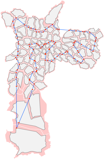
The construction of the problem started by downloading a political-administrative map of the city from the city hall website; see http://geosampa.prefeitura.sp.gov.br/. The map describes each neighborhood as a polygon. The polygon with more vertices has 5,691 vertices and, all together, the polygons have 156,852 vertices. To turn the problem into something more tractable, we redefine the polygons with number of vertices $n_{v}>100$ (all of them in fact) by considering only the vertices with indices of the form form $1+\lfloor 50/n_{v}\rfloor j$ for $j=0,1,2,\dots$. This way, all polygons were left with a number of vertices between 51 and 57, totaling 4,966 vertices. Moreover, for artistic reasons related to the graphical representation of the problem, we shrunk each polygon by 20%. The shrinkage consisted in replacing each vertex $v_{i}$ by $o_{i}+0.8(v_{i}-o_{i})$, where the offset $o_{i}=\frac{1}{2}(x_{\min}+x_{\max},y_{\min}+y_{\max})^{T}$, and $(x_{\min},y_{\min})^{T}$ and $(x_{\max},y_{\max})^{T}$ correspond to the lower-left and upper-right corners of the smallest rectangle that encloses the polygon. With this procedure we ended up with the $p=96$ polygons $\Omega_{i}$ for $i=1,\dots,p$ that determine the problem (35) under consideration; see Figure 3.

Figure 3: Representation of the $p=96$ polygons that determine problem (35). The considered polygons appear in gray, while the original polygons appear in coral on the background merely to improve the artistic appearance of the drawing.

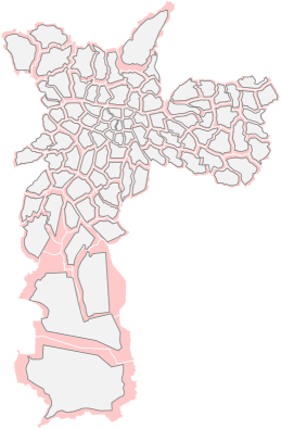
Table 1 shows the details of the optimization process. The table shows, for each iteration, the length of the current route. It also shows, for each iteration, how many neighbors had to be evaluated to find one that improves the current route. Naturally, each evaluation of a neighbor corresponds to a call to the BCD method. Therefore, the next two columns show the number of calls to the BCD method per iteration and the number of cycles these calls used. The last two columns of the table show these two values accumulated over the iterations. It can be noted from the table that the BCD method is used to solve more than 200,000 subproblems and that this requires, altogether, the execution of more than 3 million cycles, i.e. an average of 15 cycles per problem. The instance under consideration has $p=96$ points. The constructive heuristic used to generate the initial point evaluates (by calling the BCD method) $O(\frac{1}{2}p^{2})$ permutations; while the reinsertion neighborhood evaluates, in the worst case, $O(p^{2})$ neighbors. The first line of the table shows the cost of the constructive heuristic, and is consistent with what we have just mentioned. The remaining lines show that in the first 4 iterations and in a few intermediate iterations the method quickly finds a neighbor that improves the current solution. On the other hand, the average number of neighbors evaluated per iteration is 4,164, which corresponds to approximately 45% of the neighbors. The running time of the algorithm is directly proportional and totally dependent on the cost of computing $\boldsymbol{x}_{i_{k}}^{trial}$. The constructive heuristic used to compute the initial point $x^{0}$ used 29.58 seconds of CPU time; while the method as a whole consumed practically one hour of CPU time, exactly 3,589.31 seconds.

iter	Route lenght	Usage of BCD method per iter		Accumulated usage of BCD method
		# calls	# cycles	# calls	# cycles
0	229,139.65	4,653	40,018	4,653	40,018
1	227,965.59	2	26	4,655	40,044
2	227,110.10	1	10	4,656	40,054
3	226,970.07	3	56	4,659	40,110
4	226,970.07	2	24	4,661	40,134
5	226,588.08	4,125	60,955	8,786	101,089
6	226,586.52	4,418	66,454	13,204	167,543
7	226,575.05	4,220	64,793	17,424	232,336
8	226,575.05	95	1,655	17,519	233,991
9	226,573.77	4,510	66,294	22,029	300,285
10	226,573.77	189	2,658	22,218	302,943
11	226,391.25	4,708	69,757	26,926	372,700
12	226,063.02	4,789	70,987	31,715	443,687
13	224,708.13	3,653	57,797	35,368	501,484
14	224,391.45	4,889	73,541	40,257	575,025
15	224,391.45	3,747	59,159	44,004	634,184
16	224,236.40	4,801	70,928	48,805	705,112
17	224,128.38	4,983	74,453	53,788	779,565
18	224,128.38	95	1,761	53,883	781,326
19	224,128.38	95	908	53,978	782,234
20	224,100.64	3,851	58,075	57,829	840,309
21	224,100.64	3,838	57,462	61,667	897,771
22	223,681.92	4,887	75,693	66,554	973,464
23	223,261.18	3,947	66,182	70,501	1,039,646
24	223,261.18	95	847	70,596	1,040,493
25	223,242.32	5,076	77,901	75,672	1,118,394
26	223,013.14	5,572	92,531	81,244	1,210,925
27	221,526.66	5,701	91,366	86,945	1,302,291
28	221,469.25	94	900	87,039	1,303,191
29	219,846.99	5,606	89,792	92,645	1,392,983
30	219,505.59	1	4	92,646	1,392,987
31	219,096.08	5,761	92,924	98,407	1,485,911
32	218,652.50	6,164	96,849	104,571	1,582,760
33	217,719.39	6,146	97,136	110,717	1,679,896
34	216,509.74	6,256	98,403	116,973	1,778,299
35	215,372.59	6,350	99,083	123,323	1,877,382
36	214,676.14	5,289	87,276	128,612	1,964,658
37	214,674.57	5,077	82,038	133,689	2,046,696
38	214,674.57	1,345	29,796	135,034	2,076,492
39	214,102.74	3,937	71,897	138,971	2,148,389
40	214,102.74	95	1,033	139,066	2,149,422
41	213,754.48	5,190	92,893	144,256	2,242,315
42	213,533.35	6,049	98,937	150,305	2,341,252
43	213,290.76	6,241	102,045	156,546	2,443,297
44	213,231.26	7,195	115,060	163,741	2,558,357
45	213,071.95	6,338	99,378	170,079	2,657,735
46	213,070.90	6,625	103,442	176,704	2,761,177
47	213,032.17	7,297	111,568	184,001	2,872,745
48	212,773.09	7,681	116,393	191,682	2,989,138
49	212,499.29	7,585	115,190	199,267	3,104,328
50	212,292.01	8,161	125,796	207,428	3,230,124
51	212,292.01	9,120	154,558	216,548	3,384,682

Table 1: Performance of the heuristic method applied to solve the considered instance of the continuous version of the TSP problem.

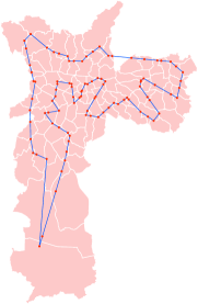
Figure 4 shows the evolution of the route length over the iterations of the method; while Figure 5 shows some of the generated routes. Figure 6 shows the final iterate in detail.

Figure 4: Route length as a function of the iteration number.

(a) 229,139.65	(b) 226,573.767	(c) 224,100.64
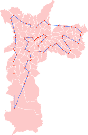(d) 219,505.59	(e) 214,102.74	(f) 212,292.01

Figure 5: Sample of the routes that are built throughout the iterative optimization process. The lenght of each route appears near to the route. The map of São Paulo city appears in the background for artistic purposes, but the polygons representing the districts are being omitted for the sake of clarity. (a) Represents the initial guess given by the constructive heuristic; (f) Represents the final iterate (obtained at iteration 51); and (b)–(e) Represent the iterands of the iterations 10, 20, 30 and 40, respectively. It is worth noting that the red dots, each always within its respective polygon that is not being displayed, move from one iteration to another.

Figure 6: Final iterate with route lenght equal to 212,292.01.

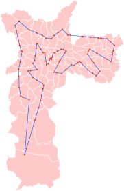
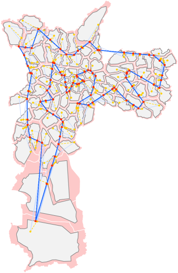
Up to this point, we have described and illustrated in detail the way in which the discrete heuristic method described in Section 6.2 made intensive use of the BCD method to solve the problem (35). We close the numerical experiments section by showing in Figure 7, with a graphic and a table, the iterands of the BCD method for a specific fixed permutation. To make this figure, we considered the permutation given by the constructive heuristic used to generate $x^{0}$ and we randomly draw points inside each of the polygons. The graph and table show the iterations for 13 complete cycles. The method actually uses 44 cycles, but the functional value varies from 229,139.66 at the end of cycle 13 to 229,139.65 at the end of cycle 44, when it stops because all the variables’ blocks are repeated from cycle 43 to cycle 44. The initial points are in yellow or light orange and the color changes to red at cycle 13. The evolution of each point is marked with a dotted line whose color changes along with the color of the point. Independently of that, the route determined by the points of each cycle is marked in blue. The route with the lightest blue corresponds to the route given by the initial points (yellow or light orange) and the color of the route gets darker and darker until it reaches the route of cycle 13, marked with the strongest blue. Roughly speaking, the points move a little more in the first 3 cycles, in which the objective function decreases the most, and then there are only small accommodations of the points until the method converges. The authors are aware of the difficulty to see the figure clearly; a zoom in the image is recommended to see the details of the evolution of the iterands. In particular, the middle left part clearly shows how the route is being modified as the points move.

Cycle Route lenght 0 425,047.86 1 244,338.54 2 232,471.73 3 230,402.57 4 229,223.98 5 229,171.84 6 229,142.28 7 229,140.84 8 229,140.22 9 229,139.93 10 229,139.79 11 229,139.72 12 229,139.68 13 229,139.66

Figure 7: Sequence of iterands of the BCD method when applied to random initial points within the polygons and with the order given by the constructive heuristic used to generate the initial point.

7 Conclusions

The framework presented in the present work could be extended in order to consider Taylor-like high-order models [4] satisfying well-established regularity assumptions, as it has been done in [2] for the case of box constraints. However, theoretical results in [2] reveal that using high-order models associated with Coordinate Descent methods is not worthwhile. The reason is that overall computed work is dominated by the necessity of obtaining fast decrease of the distance between consecutive iterates, whereas high-order models do not help for achieving such purpose.

More interesting, from the practical point of view, is to exploit the particular case in which the constraints that define each $\Omega_{i}$ may be expressed in the form of global inequalities and equalities. (Of course, this is a particular case of the one addressed in this paper that corresponds to set $n_{\mathrm{ops}}(i)=1$ for all $i=1,\ldots,n_{\mathrm{blocks}}$.) In this case the obvious choice for solving subproblems consists of using some well established constrained optimization software. From the theoretical point of view there is nothing to be addded, since practical optimization methods for constrained optimization may fail for different reasons, leading the abrupt interruption of the overall optimization process. However, we have no doubts that in many practical problems the standard constrained optimization approach associated with block coordinate descent should be useful.

The reason why, in this paper, we considered feasible sets $\Omega_{i}$ with the local constrained structure defined by open covering sets and constitutive constraints is not strictly related to block coordinate methods. In fact, in contact with several practical problems (an example of which is the one presented in Section 6) we observed that the non-global structure of constraints is not unusual and needs specific ways to be handled properly. We believe that different approaches than the one suggested in this paper are possible, most of them motivated by the particular structure of the practical problems at hand. Further research is expected in the following years with respect to this subject.

References

- [1] E. Aarts and J. K. Lenstra, (eds.) Local Search in Combinatorial Optimization, Princeton University Press, 2003.
- [2] V. A. Amaral, R. Andreani, E. G. Birgin, D. S. Marcondes, and J. M. Martínez, On complexity and convergence of high-order coordinate descent algorithms for smooth nonconvex box-constrained minimization, arXiv:2009.01811v3.
- [3] D. L. Applegate, R. E. Bixby, V. Chvátal, and W. J. Cook, The Traveling Salesman Problem: A Computational Study, Princeton University Press, 2006.
- [4] E. G. Birgin, J. L. Gardenghi, J. M. Martínez, S. A. Santos, and Ph. L. Toint, Worst-case evaluation complexity for unconstrained nonlinear optimization using high-order regularized models, Mathematical Programming 163, pp. 359–368, 2017.
- [5] E. G. Birgin and J. M. Martínez, On regularization and active-set methods with complexity for constrained optimization, SIAM Journal on Optimization 28, pp.1367–1395, 2018.
- [6] E. G. Birgin and J. M. Martínez, A Newton-like method with mixed factorizations and cubic regularization for unconstrained minimization, Computational Optimization and Applications 73, pp. 707–753, 2019.
- [7] M. Gendreau, A. Hertz, and G. Laporte, New insertion and post optimization procedures for the traveling salesman problem, Operations Research 40, pp. 1086–1094, 1992.
- [8] M. J. D. Powell , On search directions for minimization algorithms, Mathematical Programming 4, pp. 193–201, 1973.
- [9] S. J. Wright, Coordinate descent methods, Mathematical Programming 151, pp. 3–34, 2015.