Thermodynamics of stationary states of the ideal gas in a heat flow

Abstract

There is a long-standing question as to whether and to what extent it is possible to describe nonequilibrium systems in stationary states in terms of global thermodynamic functions. The positive answers have been obtained only for isothermal systems or systems with small temperature differences. We formulate thermodynamics of the stationary states of the ideal gas subjected to heat flow in the form of the zeroth, first, and second law. Surprisingly, the formal structure of steady state thermodynamics is the same as in equilibrium thermodynamics. We rigorously show that $U$ satisfies the following equation $dU=T^{*}dS^{*}-pdV$ for a constant number of particles, irrespective of the shape of the container, boundary conditions, size of the system, or mode of heat transfer into the system. We calculate $S^{*}$ and $T^{*}$ explicitly. The theory selects stable nonequilibrium steady states in a multistable system of ideal gas subjected to volumetric heating. It reduces to equilibrium thermodynamics when heat flux goes to zero.

I Introduction

Thermodynamics simplifies the description of equilibrium systems. It reduces the number of equations of state of material by expressing them with one formula in terms of a thermodynamic potential (Thermodynamics_and_an_Introduction_to_Thermostatistics_2ed_H_Callen, ). This simplification also significantly reduces the number of measurements needed to determine any material’s equilibrium properties (History_of_Thermodynamics_The_Doctrine_of_Energy_and_Entropy_by_Ingo_Muller, ). It also determines the equilibrium state of the system by optimization rules.

For similar reasons, there has been an enormous research effort to introduce global thermodynamics with optimization rules and potential-like formulation for steady states (Introduction_to_thermodynamics_of_irreversible_processes_Ilya_Prigogine, ; oono1998steady, ; sekimoto1998langevin, ; hatano2001steady, ; sasa2006steady, ; guarnieri2020non, ; boksenbojm2011heat, ; netz2020approach, ; mandal2013nonequilibrium, ; holyst2019flux, ; jona2014thermodynamics, ; speck2005integral, ; mandal2016analysis, ; maes2019nonequilibrium, ; Zhang2021continuous, ; glansdorff1964general, ; maes2014nonequilibrium, ; ruelle2003extending, ; sasa2014possible, ; komatsu2008expression, ; komatsu2008steady, ; komatsu2011entropy, ; chiba2016numerical, ; nakagawa2017liquid, ; nakagawa2019global, ; sasa2021stochastic, ; nakagawa2022unique, ). The progress in this direction is limited either to the isothermal situations or to the small temperature differences (komatsu2008expression, ; komatsu2008steady, ; komatsu2011entropy, ; chiba2016numerical, ; nakagawa2017liquid, ; nakagawa2019global, ; sasa2021stochastic, ; nakagawa2022unique, ). Here we break this limitation and show that the steady state thermodynamic description also exists for a system that is far from equilibrium (with large temperature gradients).

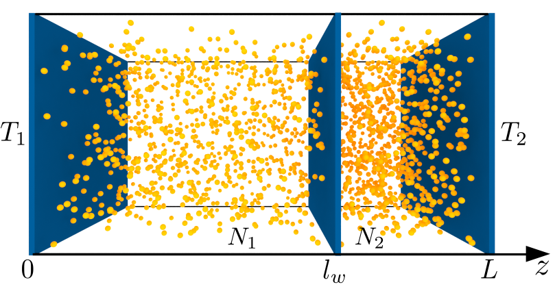
Figure 1: Schematic illustration of an ideal gas in a box with an internal wall.

For a paradigmatic system such as an ideal gas, only three parameters (entropy $S$, volume $V$, and the number of particles $N$) are sufficient to determine its state at thermal equilibrium. At a nonequilibrium state, one has to consider spatially dependent parameters, such as temperature $T\left(\mathbf{r}\right)$, pressure $p\left(\mathbf{r}\right)$, and density $n\left(\mathbf{r}\right)$. A description of such fields appears in De Groot and Mazur’s monograph on irreversible thermodynamics (Groot_Mazur_Non-equilibrium_thermodynamics, ). This description is based on local conservation laws of mass, momentum and energy. With the assumption of local equilibrium and constitutive relations, irreversible thermodynamics determines the state of the system.

In this paper, we show that within irreversible thermodynamics, there exists a global description of a steady state of an ideal gas in heat flow. Within this description the total system’s energy is represented as a function of $S^{*}$, volume $V$, and the number of particles $N$. We formulate thermodynamics of steady state in the form of the zeroth, first and second law and determine $S^{*}$ explicitly. Our scheme for thermodynamics of nonequilibrium steady states is rigorous and valid for large heat flux.

We illustrate the scheme using a monoatomic ideal gas confined between two parallel walls with different temperatures $T_{1}$ and $T_{2}$. Furthermore, we introduce to this system a constraint in the form of a thin wall separating the gas into two parts, as shown in Fig. 1. We assume that this internal wall is diathermic and impenetrable. Considering the system with internal constraints puts our problem in the perspective of equilibrium thermodynamics as described by Callen ‘The single, all-encompassing problem of thermodynamics is the determination of the equilibrium state that eventually results after the removal of internal constraints in a closed, composite system’ (Thermodynamics_and_an_Introduction_to_Thermostatistics_2ed_H_Callen, ). We show the minimum principle that determines the stable position of the internal wall.

This description also applies to different shapes of the system, boundary conditions, and different modes of heat transfer (heat flows through the system or heat is generated inside the system) and is valid beyond the regime of linear irreversible thermodynamics, thus taking into account the temperature-dependent heat conductivity.

II Ideal gas in heat flow

We consider a fluid described by irreversible thermodynamics (Groot_Mazur_Non-equilibrium_thermodynamics, ). Therefore, the gas is described by five equations: two local equations of state and three conservation laws (continuity equation, Navier-Stokes equation, and the energy balance equation) supplemented by proper boundary conditions. We assume that the equation of state corresponds to the monoatomic ideal gas. The gas is confined between two parallel walls at positions $0$ and $L$. We assume that the system is translationally invariant in $x,y$ directions. Moreover, the gas satisfies local equilibrium and is described by the following equations of state (Thermodynamics_and_an_Introduction_to_Thermostatistics_2ed_H_Callen, )

$$p\left(z\right)=n\left(z\right)k_{B}T\left(z\right),$$ (1)

with Boltzmann constant $k_{B}$, pressure $p\left(z\right)$, particle number density $n\left(z\right)$, and the temperature $T\left(z\right)$ at position $z$. It is worth mentioning that the local equilibrium is sometimes questioned. But as we discuss in the conclusions section, for an ideal gas the local equilibrium is valid up to extreme temperature gradients of the order of $10^{7}K/cm$. The energy equation of state is given by

$$\epsilon\left(z\right)=\frac{3}{2}n\left(z\right)k_{B}T\left(z\right).$$ (2)

Here $\epsilon\left(z\right)$ is the internal energy volumetric density. We also assume that in the whole volume $V=AL$, where $A$ is an area (along $x,y$) direction, there are $N$ particles. The boundary condition follows from the assumption of a given temperature on the walls

$$T\left(0\right) =T_{1},$$

$$T\left(L\right) =T_{2}.$$ (3)

In the stationary state, the system is described by $T_{1},T_{2},A,L,N$, which we call the control parameters. We assume that there is no mass flow for the confined gas in a stationary state. That simplifies the thermohydrodynamic equations (Groot_Mazur_Non-equilibrium_thermodynamics, ). The Navier-Stokes equation is reduced to a condition of vanishing pressure gradient, $\nabla p\left(z\right)=0.$ The two equations of state follow that the energy density is also constant in space and $\epsilon=3p/2$. The total energy $U$ is thus given by $U=A\int_{0}^{L}dz\,\epsilon=3ALp/2$. We rewrite this expression in terms of the volume of the system, $V$ , obtaining the relation between pressure and volume,

$$p=\frac{2}{3}\frac{U}{V}.$$ (4)

The energy balance equation with the Fourier law for the heat flux,

$$J_{q}=-\kappa\nabla T\left(z\right),$$ (5)

gives $0=\kappa\frac{d^{2}}{dz^{2}}T\left(z\right).$ With the boundary conditions (3), it yields a linear temperature profile, $T\left(z\right)=T_{1}+\left(T_{2}-T_{1}\right)z/L$. With the constant pressure and the equation of state, it determines density profile, $n\left(z\right)=p/k_{B}T\left(z\right)$, and with a given number of particles, $N=A\int_{0}^{L}dz\,n\left(z\right)$, they determine pressure,

$$p=\frac{N}{V}k_{B}\frac{T_{2}-T_{1}}{\log\frac{T_{2}}{T_{1}}}.$$ (6)

Suppose that the system is in the stationary state described by parameters $T_{1},T_{2},A,L,N$. Then we start changing the temperature $T_{2}$ to $T_{2}+dT_{2}$. After a while the system reaches another stationary state, this time described by parameters $T_{1},T_{2}+dT_{2},A,L,N$. We could similarly move one of the system’s walls and change its length $L\to L+dL$. The disturbance of the system induces time-dependent thermo-hydrodynamic flows. They may be complex (with sound waves, turbulent motion or heat front zuk2022transient ) if the change of the temperature or position of the wall is sudden. Nevertheless, the possibility of solving thermohydrodynamic equations would allow one to monitor the change of the internal energy $dU$, the net heat $\mkern 3.0mu\mathchar 22\relax\mkern-12.0mudQ$ entering the system during the transition, and the work done $\mkern 3.0mu\mathchar 22\relax\mkern-12.0mudW$. Independently of the rate of change of the control parameters, the energy balance within irreversible thermodynamics must have the following consequences in the context of passing from one to another stationary state,

$$dU=\mkern 3.0mu\mathchar 22\relax\mkern-12.0mudW+\mkern 3.0mu\mathchar 22\relax\mkern-12.0mudQ.$$ (7)

The energy change is determined by the control parameters through equations (4) and (6). As in similar considerations within equilibrium thermodynamics, the work and heat of the transitions between steady states depend on the transition rate. However, there is an essential simplification for the case of slow processes (oono1998steady, ). We expect, that the slow change of the boundary condition does not disturb the homogeneity of the pressure in the system. In the limit of slow changes, the work done in the transition is given by

$$\mkern 3.0mu\mathchar 22\relax\mkern-12.0mudW =-pdV,$$ (8)

where $dV$ denotes the differential of the volume of the system. Therefore the net heat differential is determined from (7) and (8) by

$$\mkern 3.0mu\mathchar 22\relax\mkern-12.0mudQ=dU+pdV.$$ (9)

We prove it below using thermo-hydrodynamic equations. The above equation represents the energy balance in the system. It may be called the first law because it has a form of and it reduces to the first law of equilibrium thermodynamics when the heat does not flow through the gas.

III The first law for stationary states in the case of thermohydrodynamics

The total internal energy of the gas at given time instant, $U_{i}\left(t\right)$, in volume $V\left(t\right)$ is given by the following integration of its density,

$$U_{i}\left(t\right)=\int_{V(t)}d^{3}r\,\rho\left({\bf r},t\right)u\left({\bf r},t\right),$$ (10)

where $\rho\left({\bf r},t\right)$ is the density and $u\left({\bf r},t\right)$ is the internal energy density per unit mass at position ${\bf r}$ and time $t$. To facilitate our considerations, but without loss of generality, we assume the translational invariance of the system in $x,y$ directions. Before time $t_{i}$ the system is in a stationary state. Then, due to a change of volume $V$, temperatures $T_{1}$, $T_{2}$, or other external factors, the system is taken to another nearby stationary state, which is achieved after $t_{f}$. For example, between times $t_{i}$ and $t_{f}$ we slowly change the position of the right wall by manipulating its position, $L\left(t\right)$, such that initially $L\left(t_{i}\right)=L$ changes to $L\left(t_{f}\right)=L+dL$. That gives the time dependent volume, $V\left(t\right)=AL\left(t\right)$, with the total change $dV=AdL$ when passing from the stationary state at $t_{i}$ to the stationary state at $t_{f}$. Differential of the energy (i.e. small change of the energy when passing to neighboring stationary state) is given by,

$$dU=U_{i}\left(t_{f}\right)-U_{i}\left(t_{i}\right),$$

which we equivalently express as,

$$dU=\int_{t_{i}}^{t_{f}}dt\,\frac{dU_{i}\left(t\right)}{dt}.$$ (11)

With the use of Eq. (10) we get $dU_{i}/dt=\frac{d}{dt}\int_{V(t)}d^{3}r\,\rho\left({\bf r},t\right)u\left({\bf r},t\right)$. In this expression, the integral is simplified with the use of $x,y$ translational symmetry and keeping in mind, that $V\left(t\right)=AL\left(t\right)$ as follows,

$$\int_{V(t)}d^{3}r\,\rho\left({\bf r},t\right)u\left({\bf r},t\right)=A\int_{0}^{L\left(t\right)}dz\,\rho\left(z,t\right)u\left(z,t\right),$$

so the time derivative of internal energy reduces to

$$\frac{dU_{i}}{dt} =A\frac{d}{dt}\int_{0}^{L\left(t\right)}dz\,\rho\left(z,t\right)u\left(z,t\right)$$

$$=A\rho\left(L\left(t\right),t\right)u\left(L\left(t\right),t\right)\frac{dL\left(t\right)}{dt}$$

$$+A\int_{0}^{L\left(t\right)}dz\,\frac{\partial}{\partial t}\left[\rho\left(z,t\right)u\left(z,t\right)\right].$$ (12)

In the latter integral there appears the left-hand side of the balance energy equation (cf. p. 18 in (Groot_Mazur_Non-equilibrium_thermodynamics, ))

$$\frac{\partial}{\partial t}\left[\rho\left(z,t\right)u\left(z,t\right)\right] =-div\left(\rho\left(z,t\right)u\left(z,t\right){\bf v}\left(z,t\right)+{\bf J}_{q}\right),$$

$$-{\bf P}:grad{\bf v}\left(z,t\right)$$ (13)

with velocity field ${\bf v}\left(z,t\right)$, heat flow $\boldsymbol{J}_{q}$ and pressure tensor ${\bf P}=p\left(z,t\right){\bf I}+$${\bf\Pi}$, where ${\bf I}$ is the unit 3-dimensional matrix and ${\bf\Pi}$ is proportional to velocity gradients. Due to the fact, that there is no velocity field in the system in stationary state, and the change of the parameters is slow, we keep only the leading terms in velocity field in the above expression, neglecting the quadratic term, ${\bf\Pi}:grad{\bf v}\left(z,t\right)\approx 0$. Therefore ${\bf P}:grad{\bf v}\left(z,t\right)\approx p\left(z,t\right)\,div{\bf v}\left(z,t\right)$ and the energy balance equation simplifies to

$$\frac{\partial}{\partial t}\left[\rho\left(z,t\right)u\left(z,t\right)\right]=$$

$$-div\left(\rho\left(z,t\right)u\left(z,t\right){\bf v}\left(z,t\right)+{\bf J}_{q}\right)-p\left(z,t\right)\,div{\bf v}\left(z,t\right).$$

Using the above in expression (12) we obtain

$$\frac{dU_{i}}{dt} =A\rho\left(L\left(t\right),t\right)u\left(L\left(t\right),t\right)\frac{dL(t)}{dt}$$

$$-A\int_{0}^{L\left(t\right)}dz\,div\left(\rho\left(z,t\right)u\left(z,t\right){\bf v}\left(z,t\right)\right)+$$

$$-A\int_{0}^{L\left(t\right)}dz\,div{\bf J}_{q}-A\int_{0}^{L\left(t\right)}dz\,p\left(z,t\right)\,div{\bf v}\left(z,t\right).$$

The first two terms on the right-hand side give zero, because

$$\int_{0}^{L\left(t\right)}dz\,div\left(\rho\left(z,t\right)u\left(z,t\right){\bf v}\left(z,t\right)\right)=$$

$$\rho\left(L\left(t\right),t\right)u\left(L\left(t\right),t\right){\bf v}_{z}\left(L\left(t\right),t\right)-\rho\left(0,t\right)u\left(0,t\right){\bf v}_{z}\left(0,t\right)$$

and because $z$-component of the velocity above vanishes for $z=0$ and is equal to $dL\left(t\right)/dt$ for $z=L$. The third term, $A\int_{0}^{L\left(t\right)}dz\,div{\bf J}_{q}=\int_{V\left(t\right)}d^{3}r\,div{\bf J}_{q}$ is the total heat rate that flows to the system which is evident after application of Gauss theorem, $\int_{V\left(t\right)}d^{3}r\,div{\bf J}_{q}=\int_{\partial V\left(t\right)}d^{2}r\,{\bf n}\cdot{\bf J}_{q}$. Here, ${\bf n}$ is the normal vector pointing outside the surface. We denote the heat rate flowing into the system by

$$q\left(t\right)\equiv-\int_{\partial V\left(t\right)}d^{2}r\,{\bf n}\cdot{\bf J}_{q}.$$ (14)

To simplify the fourth term we use the fact, that pressure in the system during slow change of parameters is still homogeneous, $p\left(z,t\right)=p\left(t\right)$, therefore $\int_{0}^{L\left(t\right)}dz\,p\left(z,t\right)\,div{\bf v}\left(z,t\right)=Ap\left(t\right)\int_{0}^{L\left(t\right)}dz\,\,div{\bf v}\left(z,t\right)$. This integral is the volume change rate, $dV\left(t\right)/dt=\int_{V\left(t\right)}d^{3}r\,\,div{\bf v}\left(z,t\right)$ and finally for the fourth term we get, $A\int_{0}^{L\left(t\right)}dz\,p\left(z,t\right)\,div{\bf v}\left(z,t\right)=p\left(t\right)dV\left(t\right)/dt.$ Therefore the change of the energy (12) simplifies to

$$\frac{dU_{i}}{dt}=q\left(t\right)-p\left(t\right)\frac{dV\left(t\right)}{dt}.$$

Utilizing the above in expression (11) we obtain,

$$dU=\int_{t_{i}}^{t_{f}}dt\,q\left(t\right)-\int_{t_{i}}^{t_{f}}dt\,p\left(t\right)\frac{dV\left(t\right)}{dt}.$$ (15)

We use the dominant term for small changes of parameters (neighboring stationary state) in $\int_{t_{i}}^{t_{f}}dt\,p\left(t\right)\frac{dV\left(t\right)}{dt}\approx p\int_{t_{i}}^{t_{f}}dt\,\frac{dV\left(t\right)}{dt}=pdV.$ The above energy differential may be written in the form of (7) where

$$\mkern 3.0mu\mathchar 22\relax\mkern-12.0mudQ=\int_{t_{i}}^{t_{f}}dt\,q\left(t\right)$$

is the total heat transfer to the system and $\mkern 3.0mu\mathchar 22\relax\mkern-12.0mudW=-pdV$ is the work performed on the system during the transition between stationary states.

It is worth noting that in the above derivation, we did not specify temperature changes. Therefore the energy balance (7) is valid for transitions in the space of $V,T_{1},T_{2}$. Eq. (7) derived above is valid under the assumption of slow changes of external parameters (including homogeneous pressure condition). In this limit it is a rigorous expression. Therefore, if $q\left(t\right)=0$ in a stationary state (before $t_{i}$ and after $t_{f}$) and both $dU$, $\mkern 3.0mu\mathchar 22\relax\mkern-12.0mudW$ are finite and well defined (which is exactly the case considered here), then the net heat, $\mkern 3.0mu\mathchar 22\relax\mkern-12.0mudQ$, transferred to the system during the transition is finite and well defined as well.

IV nonequilibrium entropy as a potential of the net heat differential

It is worth noting that the net heat introduced above would be the excess heat considered by Oono and Paniconi (oono1998steady, ). In what follows, we are going to find the integrating factor and the related potential. As we will see, they define the nonequilibrium temperature and $S^{*}$, which may be called a nonequilibrium thermodynamic entropy.

Before proceeding further, it is worth giving several comments. First, for constant $N,$ four parameters determine the state of the system, $T_{1},T_{2},A,L$. So the Pfaff form for the heat (9) may be written in the space of these parameters in terms of $dT_{1}$, $dT_{2}$ , $dA$, and $dL$. Second, because the pressure in the system is homogeneous, we can write the expression for elementary work, $\mkern 3.0mu\mathchar 22\relax\mkern-12.0mudW=-pAdL-pLdA$, which we shortly write in terms of the volume of the system, $\mkern 3.0mu\mathchar 22\relax\mkern-12.0mudW=-pdV$. Third, once the integrating factor and the corresponding potential are found, it is straightforward to represent them in another set of variables of states. It is easy to check, that the integrating factor in variables $X$, denoted by $\lambda_{x}\left(X\right)$, after changing the variables of states to $Y$ given by $Y\left(X\right)$, transforms to $\lambda_{y}\left(Y\right)=\lambda_{x}\left(X\left(Y\right)\right)$. Similar holds for the potential corresponding to the integrating factor. We work in variables $U,V,T_{2}/T_{1}$. In these variables, the heat differential (9) is given by,

$$\mkern 3.0mu\mathchar 22\relax\mkern-12.0mudQ=dU+\frac{2}{3}\frac{U}{V}dV+0\cdot d\frac{T_{2}}{T_{1}},$$ (16)

where we explicitly wrote the vanishing third term to remind that the form is in three-dimensional space, $U,V,T_{2}/T_{1}$ and used expression (4) for pressure.

We observe that the heat differential (16) in variables $U,V,T_{2}/T_{1}$ is identical to the heat differential for an ideal gas in equilibrium thermodynamics (Thermodynamics_and_an_Introduction_to_Thermostatistics_2ed_H_Callen, ). This is a consequence of the fact that both in equilibrium thermodynamics and in the nonequilibrium stationary state considered here, the energy is exchanged in two same ways (heat and mechanical work) and that the relationship between pressure and internal energy for equilibrium ideal gas, $p=2U/3V$, is identical to formula (4). Therefore, the heat differential has an integrating factor $T^{*}\left(U,V,T_{2}/T_{1}\right)$ and the corresponding potential, $S^{*}\left(U,V,T_{2}/T_{1}\right)$,

$$\mkern 3.0mu\mathchar 22\relax\mkern-12.0mudQ=T^{*}dS^{*}.$$ (17)

The integrating factor and the potential are not unique. To find the integrating factor we observe that formula (16) is the thermodynamics first law for a monoatomic ideal gas in equilibrium thermodynamics. In this case, the integrating factor is the temperature of the system, which for an ideal gas is given by the formula $T=2U/3Nk_{B}$. For the nonequilibrium case considered here, we introduce a similar expression, so the integrating factor is given by

$$T^{*}=\frac{2U}{3Nk_{B}}.$$ (18)

The potential corresponding to the above integrating factor is $S^{*}$. As follows from (16), (17) and (18), the differential of $S^{*}$ is given by,

$$dS^{*}=\frac{3Nk_{B}}{2U}dU+\frac{Nk_{B}}{V}dV.$$

$S^{*}$ is thus given by the following formula, $S^{*}\left(U,A,L,T_{2}/T_{1}\right)=Nk_{B}\log\left(U^{3/2}V\right)+S_{0},$ where $S_{0}$ is a numeric constant. However, it may depend on parameters of the system which are not treated as the variables of state, including the number of particles $N$, which we set to be constant in the above reasoning. We determine $S_{0}$ constant by the condition that $S^{*}$ for $T_{2}=T_{1}$ gives the equilibrium expression (Thermodynamics_and_an_Introduction_to_Thermostatistics_2ed_H_Callen, ). Therefore we get,

$$S^{*}\left(U,V,T_{2}/T_{1}\right)=Nk_{B}\left\{\frac{5}{2}+\frac{3}{2}\log\left[\frac{2}{3}\frac{\varphi_{0}U}{N}\left(\frac{V}{N}\right)^{2/3}\right]\right\},$$ (19)

where $\varphi_{0}$ is a constant that does not depend on any control parameter. The above fundamental relation has proper partial derivatives,

$$\left(\frac{\partial S^{*}}{\partial U}\right)_{V,N} =\frac{1}{T^{*}},$$ (20)

$$\left(\frac{\partial S^{*}}{\partial V}\right)_{U,N} =\frac{p}{T^{*}}.$$

As a potential of the heat differential, the above $S^{*}$ determines stationary-state adiabats (oono1998steady, ). They are different from adiabats defined in equilibrium. Because $S^{*}$ does not depend on the temperature ratio, we see that the change of $T_{2}/T_{1}$ (keeping $U,A,L$, and $N$ constant) changes the temperature profile in the system. It also changes the heat flowing through the system. But it does not trigger the exchange of the net heat. As we show below, $T_{2}/T_{1}$ is a parameter that controls the entropy production in the system.

There is a natural question about the relation between $S^{*}$ and the total entropy of the system, $S_{\text{tot}}=A\int dz\,s\left(z\right)$, where $s\left(z\right)$ is the volumetric entropy density

$$s\left(z\right)=n\left(z\right)k_{B}\left\{\frac{5}{2}+\frac{3}{2}\log\left[\varphi_{0}k_{B}T\left(z\right)\left[n\left(z\right)\right]^{-2/3}\right]\right\},$$ (21)

as given by local equilibrium assumption within irreversible thermodynamics (Groot_Mazur_Non-equilibrium_thermodynamics, ; Thermodynamics_and_an_Introduction_to_Thermostatistics_2ed_H_Callen, ). With the use of the linear temperature profile and density determined above, we obtain,

$$S_{\text{tot}}\left(U,V,\frac{T_{2}}{T_{1}}\right) =S^{*}\left(U,V\right)+\Delta S\left(U,V,\frac{T_{2}}{T_{1}}\right),$$ (22)

$$\Delta S\left(U,V,T_{2}/T_{1}\right) =Nk_{B}\log\left[\left(\frac{T_{2}}{T_{1}}\right)^{5/4}\left(\frac{\log\frac{T_{2}}{T_{1}}}{\frac{T_{2}}{T_{1}}-1}\right)^{5/2}\right].$$

The above expression is symmetric with respect to the interchange of $T_{1}$ and $T_{2}$. Only $S^{*}$ contains information about heat absorbed/released in the system (see Eqs (9,17)) on top of the dissipative background (temperature profile). $\Delta S$, on the other hand, controls the dissipative background since it depends on the entropy production given by (Groot_Mazur_Non-equilibrium_thermodynamics, ) $\sigma=-A\int_{0}^{L}dz\,\kappa\nabla T\left(z\right)\cdot\nabla\frac{1}{T\left(z\right)}=\frac{A\kappa}{L}\left(\frac{T_{2}}{T_{1}}+\frac{T_{1}}{T_{2}}-2\right)$. The difference between the total entropy and $S^{*}$ vanishes, $\Delta S\left(U,A,L,T_{2}/T_{1}\right)\to 0$, when the system approaches the equilibrium state, $T_{2}/T_{1}\to 1$. Therefore, the $S^{*}$ becomes in this limit the equilibrium entropy.

The relation between the equilibrium entropy and $S^{*}$ also sheds light on the role of $T_{2}/T_{1}$ parameter. For an “adiabatically” insulated system determined by condition $S^{*}=const$, the parameter $T_{2}/T_{1}$ changes the total entropy of the system. The change of the total entropy of the system is associated with the local heat transfer and work between different subparts of the nonequilibrium system, even if no work is performed on the system and no net heat enters it.

V Zeroth and second law for nonequilibrium stationary states

In the above, we showed that a net heat potential, nonequilibrium entropy $S^{*}$, exists for the system without a separating wall. Here we consider the existence of the potential in the context of the system from Fig. 1 with an internal wall. It is a diathermic wall that separates the gas. We assume that the wall is at position $l_{w}$ and there are $N_{1}$ particles to the left and $N_{2}=N-N_{1}$ particles to the right of the wall. An external force, $F_{w},$ can move the wall, and some work is related when the wall moves. As before, the system is described by thermohydrodynamic equations, this time with additional boundary conditions on the surface of the separating wall. At the stationary state, the pressure is homogeneous in each subsystem, but they may be different due to the action of the force on the wall. In the stationary state $F_{w}=-A\left(p_{2}-p_{1}\right)$. We assume that the wall is diathermic, so the temperature profile is the same as for the system without the wall. The temperature profile does not depend on the action of the force on the wall. We notice that each subsystem looks like the system without the wall, although with different parameters, so we can use formulas for the system without the wall to describe the system with the wall.

We describe the system’s energy with the wall using the state variables for each subsystem, $U\left(S_{1}^{*},V_{1},N_{1},S_{2}^{*},V_{2},N_{2}\right)=U_{1}\left(S_{1}^{*},V_{1},N_{1}\right)+U_{2}\left(S_{2}^{*},V_{2},N_{2}\right)$. The additivity of the energy is inscribed in the used thermohydrodynamic equations. But the additivity of entropy is a postulate of equilibrium thermodynamics. The nonequilibrium entropy $S^{*}$ is not additive for a nonequilibrium system with heat flow. If the entropy was additive, then expression $\Gamma\left(U_{1},U_{2},V_{1},V_{2},N_{1},N_{2}\right)\equiv S^{*}\left(U_{1}+U_{2},V_{1}+V_{2},N_{1}+N_{2}\right)-S^{*}\left(U_{1},V_{1},N_{1}\right)-S^{*}\left(U_{2},V_{2},N_{2}\right)$ would identically be zero. Here

$$S^{*}\left(U,V,N\right)\equiv Nk_{B}\left\{\frac{5}{2}+\frac{3}{2}\log\left[\frac{2}{3}\frac{\varphi_{0}U}{N}\left(\frac{V}{N}\right)^{2/3}\right]\right\}$$ (23)

in agreement with Eq. (19). It is cumbersome to show by explicit calculations that $\Gamma$ does not vanish. Instead, we calculate the following expression,

$$\frac{\partial}{\partial U_{2}}\left[\left(U_{1}+U_{2}\right)U_{1}\left(\frac{\partial\Gamma}{\partial U_{1}}\right)\right]=-\frac{3}{2}N_{1}k_{B},$$

which proves, that $\Gamma$ cannot vanish identically. Therefore $S^{*}\neq S_{1}^{*}+S_{2}^{*}$ for most states, and the nonequilibrium entropy is not additive.

One can wonder why the nonequilibrium entropy is not additive. Yet the nonequilibrium entropy of each subsystem is given by the same formula for the equilibrium situation, i.e. Eq. (23). In equilibrium, the zeroth law of thermodynamics would allow us to introduce the additive entropy of the whole system when the entropy of two subsystems is known. The total heat differential is given by, $\mathchar 22\relax\mkern-12.0mudQ=\mathchar 22\relax\mkern-12.0mudQ_{1}+\mathchar 22\relax\mkern-12.0mudQ_{2}=T_{1}dS_{1}+T_{2}dS_{2}$. This heat differential in the space of parameters $U_{1},V_{1},N_{1},U_{2},V_{2},N_{2}$ has no integrating factor. But the zeroth law imposes the condition of equal temperatures, $T_{1}=T_{2}\equiv T$, simplifying the heat differential to, $\mathchar 22\relax\mkern-12.0mudQ=T\left(dS_{1}+dS_{2}\right)$. We see that the function $S$ defined by $S\equiv S_{1}+S_{2}$ is a potential of heat with the temperature $T$ as the integrating factor. That is how the equilibrium zeroth law leads to the additivity of entropy.

For a nonequilibrium system, there is no equality of subsystems’ temperatures. The equilibrium zeroth law of thermodynamics is broken. However, let’s introduce the following condition called the "zeroth law of global stationary thermodynamics" for the ideal gas with a heat flow in the following form,

$$T_{2}^{*}=rT_{1}^{*}.$$ (24)

with a constant parameter $r$. With the above zeroth law condition, the net heat differential is given by $\mathchar 22\relax\mkern-12.0mudQ=T_{1}^{*}dS_{1}^{*}+rT_{1}^{*}dS_{2}^{*}.$ It appears that it has an integrating factor that is easy to guess. Defining a function

$$S_{12}^{*}\equiv S_{1}^{*}+rS_{2}^{*}$$ (25)

allows us to represent the above heat differential by

$$\mathchar 22\relax\mkern-12.0mudQ=T_{1}^{*}dS_{12}^{*}.$$

For every given nonequilibrium temperature ratio $r$, which appears in the zeroth law condition (24), the above nonequilibrium entropy $S_{12}^{*}$ splits the space of thermodynamic parameters $U_{1},V_{1},N_{1},U_{2},V_{2},N_{2}$ on adiabatically insulated subspaces parametrized by $S_{12}^{*}$.

We are now in a position to verify whether the nonequilibrium entropy $S_{12}^{*}$ can be used to generalize the equilibrium minimum energy principle to the case with the heat flow. We check whether the minimization of the energy for constant nonequilibrium entropy $S_{12}^{*}$ leads to the proper position of a movable wall. The verification requires assuming a constant number of particles, $N_{1},N_{2}$, total volume, $V=V_{1}+V_{2},$ and nonequilibrium entropy $S_{12}^{*}$ given by (25) and calculate the minimum of the total energy,

$$U_{\text{tot}}\left(S_{1}^{*},V_{1}\right)\equiv$$

$$U_{1}\left(S_{1}^{*},V_{1},N_{1}\right)+U_{2}\left(\frac{1}{r}\left(S_{12}^{*}-S_{1}^{*}\right),V-V_{1},N_{2}\right),$$ (26)

where

$$U_{1}\left(S_{1}^{*},V_{1},N_{1}\right)=\frac{3}{2\varphi_{0}}N_{1}\left(\frac{V_{1}}{N_{1}}\right)^{-\frac{2}{3}}\exp\left[\frac{S_{1}^{*}}{N_{1}k_{B}}-\frac{5}{3}\right]$$ (27)

and is obtained from Eq. (23). $U_{2}$ is given by a similar formula. The total energy in Eq. (26) have two independent parameters, $S_{1}^{*}$ and $V_{1}$. The minimum of the above energy requires the vanishing of the derivatives over the two independent parameters, which gives

$$T_{1}^{*}-\frac{1}{r}T_{2}^{*} =0,$$

$$p_{1}-p_{2} =0.$$ (28)

The above two equations determine the two independent parameters. From thermohydrodynamics, we know that the equality of pressures is the proper condition for the position of the movable wall. Equivalently, the vanishing of the derivatives of $U_{\text{tot}}\left(S_{1}^{*},V_{1}\right)$ leads to,

$$V_{1} =\frac{V}{N_{2}\left(\frac{r}{N_{1}}+\frac{1}{N_{2}}\right)},$$

$$S_{1}^{*} =\frac{N_{1}}{N_{1}+rN_{2}}S_{12}^{*}-\frac{5}{2}k_{B}\frac{rN_{1}N_{2}}{N_{1}+rN_{2}}\log r.$$ (29)

It follows that for positive $r,$ arbitrary entropy $S_{12}^{*}$, and fixed $N_{1},N_{2}$ and $V$, there is at most one point in space $S_{1}^{*}$,$V_{1}$ with vanishing derivatives. Because of the simple form of $U_{\text{tot}}$, it is easy to show that $S_{1}^{*}$ and $V_{1}$ given by Eqs. (29) are at the global minimum. It proves that the equilibrium minimum energy principle generalizes to the case with heat flow.

The above application of the “second law” requires constant $N_{1},N_{2},V=V_{1}+V_{2}$, the nonequilibrium temperature ratio $r$ and the nonequilibrium entropy $S_{12}^{*}$. To realize it experimentally, one has to know the boundary temperatures $T_{1}$ and $T_{2}$ as a function of $S_{12}^{*},r,V_{1},V,N_{1}$ and $N_{2}$. Utilizing Eqs. (4), (6) and (18) leads to the following nonequilibrium temperatures for both subsystems,

$$T_{1}^{*} =\frac{\frac{V_{1}}{V}\left(T_{2}-T_{1}\right)}{\log\left(\frac{T_{1}+\frac{V_{1}}{V}\left(T_{2}-T_{1}\right)}{T_{1}}\right)},$$

$$T_{2}^{*} =\frac{\left(1-\frac{V_{1}}{V}\right)\left(T_{2}-T_{1}\right)}{\log\left[\frac{T_{2}}{T_{1}+\frac{V_{1}}{V}\left(T_{2}-T_{1}\right)}\right]}.$$

Using the above expressions in zeroth law condition (24), we obtain

$$\left(1-\frac{V_{1}}{V}\right)\log\left[1+\frac{V_{1}}{V}\left(\tau-1\right)\right]=r\frac{V_{1}}{V}\log\left[\frac{\tau}{1+\frac{V_{1}}{V}\left(\tau-1\right)}\right],$$

with the boundary temperatures ratio $\tau=T_{2}/T_{1}$. The above relation implicitly determines the boundary temperature ratio as a function of $V_{1}/V$, i.e. $\tau=\tau\left(V_{1}/V\right).$ Because this relation is implicit, it is impossible to determine $T_{1}\left(S_{12}^{*},r,V_{1},V,N_{1},N_{2}\right)$ explicitly. But having $\tau\left(V_{1}/V\right)$, we may use expressions (23), (24), (25) and (20) to determine $T_{1}\left(S_{12}^{*},r,V_{1},V,N_{1},N_{2}\right)$.

It is straightforward to generalize the above conclusions for any system shape and temperature profile. The reason for that is the fact that a particular form of the temperature profile does not play a role in the above calculations - the existence of the global steady state thermodynamics follows in the considered case from the fact that pressure is constant and it is a function of energy and volume, here $p=2U/3V$. The ideal gas in the box volumetrically heated and separated by a movable wall considered by Zhang et al. (Zhang2021continuous, ) also has these properties. Therefore, the steady state global thermodynamics formulated here also holds for Zhang et al. (Zhang2021continuous, ) system, describing the continuous phase transition they consider. We describe Zhang et al. case in the next section.

VI Ideal gas under volumetric heat supply

For the volumetrically heated gas the heat rate in Eq. (14) does not vanish in stationary state, $q\left(t\right)\neq 0$. Zhang et al. (Zhang2021continuous, ) consider ideal gas with uniform volumetric heating $\lambda$. In this case, in the energy balance (13) there appears the source term $\lambda$ on the right-hand side. As a consequence, Eq. (15) is modified in the following way, $dU=\int_{t_{i}}^{t_{f}}dt\,q\left(t\right)-\int_{t_{i}}^{t_{f}}dt\,p\left(t\right)\frac{dV\left(t\right)}{dt}+\lambda\int_{t_{i}}^{t_{f}}dt\,V\left(t\right),$ where, as before, we take the dominant term in, $\int_{t_{i}}^{t_{f}}dt\,p\left(t\right)\frac{dV\left(t\right)}{dt}\approx pdV$, and obtain,

$$dU=\int_{t_{i}}^{t_{f}}dt\,q\left(t\right)-pdV+\lambda\int_{t_{i}}^{t_{f}}dt\,V\left(t\right).$$

Using the above and defining

$$\mkern 3.0mu\mathchar 22\relax\mkern-12.0mudQ=\int_{t_{i}}^{t_{f}}dt\,q\left(t\right)+\lambda\int_{t_{i}}^{t_{f}}dt\,V\left(t\right)$$ (30)

we obtain Eq. (7). It is worth commenting on the fact that for $\lambda\neq 0$, both the net heat $\int_{t_{i}}^{t_{f}}dt\,q\left(t\right)$ and the second term in the right-hand side of the above expression are infinite in the limit of long transition between two neighboring stationary states. However, their sum is finite. In this system, the heat constantly flows out of the system, $q\left(t\right)\neq 0$. The outflow is balanced by the generation of heat within the system as given by the heat generation rate, $\lambda V\left(t\right)$. In Oono and Paniconi (oono1998steady, ) terminology, $\mkern 3.0mu\mathchar 22\relax\mkern-12.0mudQ$ is the excess heat, and $\lambda V\left(t\right)$ is the house-keeping heat rate. The above equation is interpreted as the “renormalization” of the heat rate to obtain the excess heat (oono1998steady, ).

Zhang et al. (Zhang2021continuous, ) considered an ideal gas between two parallel walls of area $A$ located at $z=-L$ and $z=L$. The system is translationally invariant in the $x$ and $y$ directions. The walls are kept at a fixed temperature $T_{0}$ and the energy is supplied into the system’s volume in the form of heat with the flux $J$; the supplied energy per unit time and unit volume $V=2AL$ is $\lambda=J/V$. The steady state temperature profile can be obtained from the local continuity equation of energy

$$-\kappa\dfrac{\partial^{2}}{\partial z^{2}}T(z)=\lambda$$ (31)

with the boundary conditions $T(0)=T(L)=T_{0}$, giving

$$T(z)=-\dfrac{\lambda}{2\kappa}z^{2}+\dfrac{\lambda}{2\kappa}L^{2}+T_{0}.$$ (32)

At the steady state the pressure $p$ and hence also the energy density $\epsilon$ are constant. With the use of the equation of state, this determines the density profile

$$n\left(z\right)=\frac{p}{k_{B}T\left(z\right)}=\frac{2}{3}\frac{\epsilon}{k_{B}T\left(z\right)}.$$ (33)

Using

$$N=A\int_{-L}^{L}dz\,n\left(z\right),$$ (34)

for a given number of particles $N$, the energy $U=\epsilon V$ is obtained as

$$U=\dfrac{3}{2}Nk_{B}T_{0}f(\lambda\cdot\dfrac{L^{2}}{\kappa T_{0}}),$$ (35)

where a dimensionless function $f$ is given by

$$f(x)\equiv\sqrt{x(x+2)}/(2\tanh^{-1}\sqrt{x/(x+2)}).$$ (36)

Using the volumetric entropy density of an ideal gas given by Eq. (21), we obtain

$$S_{\text{tot}}\left(U,A,L,N,\lambda\right)=S^{*}\left(U,V,N\right)+\Delta S\left(U,A,L,N,\lambda\right),$$

where $S^{*}\left(U,V,N\right)$ has a form given by the RHS of Eq. (19) and

$$\Delta S\left(U,A,L,N,\lambda\right) =-(5/2)Nk_{B}\log\left[f(\lambda\cdot\dfrac{L^{2}}{\kappa T_{0}})\right]$$

$$+(5/3)\epsilon A\int_{0}^{L}dz\,\frac{\log\left[T\left(z\right)/T_{0}\right]}{T\left(z\right)}.$$ (37)

In the above formula, $T_{0}\left(U,A,L,N,\lambda\right)$ is implicitly given by Eq. (35). The temperature profile is a quadratic function of the distance $z$, therefore the integral in the above equation cannot be expressed in terms of elementary functions. Nevertheless, as for the case discussed in the previous section, the nonequilibrium entropy differs from the total entropy in the system.

Now we introduce a movable adiabatic wall parallel to the bounding walls at $z=z_{w}$. At equilibrium, the wall is located precisely in the middle of the system $z_{w}=0$. As shown in Ref. (Zhang2021continuous, ), for small heat fluxes, the position of the wall at $z_{w}=0$ is stable. Above a critical flux, the wall moves towards one of the bounding surfaces. Let us consider the second law of nonequilibrium thermodynamics discussed above for this system. Integration of the equation of state for the ideal gas (Eq. (33)) in each subsystem 1 and 2 leads to

$$p_{1,2}=\frac{2}{3}\frac{U_{1,2}}{V_{1,2}},$$ (38)

and for each subsystem Eq. (16) is satisfied (with the replacement $T_{2}/T_{1}\rightarrow\lambda$). This implies the existence of nonequilibrium entropy and nonequilibrium temperature given by formulas (18) and (19).

Consequently, the reasoning leading to the minimum principle is the same. The only difference is that instead of two temperatures $T_{1},T_{2}$, we have here a single temperature $T_{0}$ of the confining walls and the volumetric heating rate $\lambda$. The nonequilibrium temperatures in this case are given by:

$$T_{1}^{*} =T_{0}f\left(\frac{\lambda L_{1}^{2}}{\kappa T_{0}}\right)$$

$$T_{2}^{*} =T_{0}f\left(\frac{\lambda L_{2}^{2}}{\kappa T_{0}}\right),$$ (39)

where $L_{1}=L+z_{w}$ and $L_{2}=L-z_{w}$ and the function $f$ given by (36). In this case, the minimization of energy (26) also leads to the equality of pressures. It proves that ideal gas with volumetric heating can also be described with three laws of global stationary thermodynamics introduced in the previous section.

The minimization principle introduced in the previous section also leads to a single global minimum with the zero law condition and equality of pressures given by (28). Interestingly, as discussed by Zhang et al., this system exhibits a continuous phase transition from a one stable steady state with the wall in the middle of the system to the two stable stationary states with the mirror symmetry. On the other hand, the minimization procedure leads to only one stable state. However, the zeroth law condition, $r=T_{2}^{*}/T_{1}^{*}$, breaks the symmetry. Application of formulas (39) in the zeroth law condition, $r=T_{2}^{*}/T_{1}^{*}$, leads to the conclusion that for $V_{1}<V_{2}$, the parameter $r$ takes only values $r>1$. Whereas for $V_{1}>V_{2}$, the temperature ratio satisfies $0<r<1$. Therefore, setting $r$ limits the motion of the wall to half of the system. The second stable minimum is obtained by replacing $r$ with $1/r$.

VII Conclusions

It is straightforward to generalize the above conclusions for the situation with the temperature-dependent heat conductivity, $\kappa\left(T\right),$ which is beyond the scope of linear irreversible thermodynamics. The temperature-dependent heat conductivity modifies the Fourier law (5) and the temperature profile. However, it does not affect the relation, $p=2U/3V$. Therefore, the relation (16) holds and it is possible to repeat the reasoning presented above without any changes and obtain $S^{*}$ given by Eq. (19) and the nonequilibrium temperature (18). It is worth noting that the assumption of local equilibrium for the ideal gas is valid as long as the temperature gradient is sufficiently small, $l_{fp}\left|\nabla T\right|/T\ll 1,$ for the mean free path of the molecules, $l_{fp}$ (Nonequilibrium_thermodynamics_and_its_statistical_foundations_H_J_Kreuzer, ). At the pressure of $1$ bar at room temperature, the mean free path is of the order of $l_{fp}\approx 100nm$. The local equilibrium is satisfied as long as the temperature gradient is lower than ten million Kelvins per centimeter.

We draw several conclusions from the rigorous calculations performed above within irreversible thermodynamics. Even for the system with heat flow, which is far from equilibrium (significant temperature difference), global steady state thermodynamics exist. This is for ideal gas closed in a vessel of any shape and does not depend on the mode of the heat transfer (heat flows through the system or the system is heated volumetrically). The considered examples also show that $S^{*}$ that governs the net heat is independent of the entropy production, in agreement with Eq. (22).

At least since the works of Prigogine, scientists have tried to formulate a thermodynamic-like description of nonequilibrium systems. Here we show that it exists for a stationary ideal gas with heat flow. The question remains open for interacting systems and systems with kinetic energy. From the perspective of future efforts, the case of ideal gas considered here shows that the local entropy integrated over volume is not a quantity that determines the heat in the system - a possibility discussed recently nakagawa2019global . Moreover, the considered case shows that nonequilibrium entropy, defined as heat potential, is not additive.

References

- [1] Herbert B Callen. Thermodynamics and an Introduction to Thermostatistics. John Wiley & Sons, 2006.
- [2] Ingo Müller. A history of thermodynamics: the doctrine of energy and entropy. Springer Science & Business Media, 2007.
- [3] Ilya Prigogine. Introduction to thermodynamics of irreversible processes. 1967.
- [4] Yoshitsugu Oono and Marco Paniconi. Steady state thermodynamics. Progress of Theoretical Physics Supplement, 130:29–44, 1998.
- [5] Ken Sekimoto. Langevin equation and thermodynamics. Progress of Theoretical Physics Supplement, 130:17–27, 1998.
- [6] Takahiro Hatano and Shin-ichi Sasa. Steady-state thermodynamics of langevin systems. Physical review letters, 86(16):3463, 2001.
- [7] Shin-ichi Sasa and Hal Tasaki. Steady state thermodynamics. Journal of statistical physics, 125(1):125–224, 2006.
- [8] Giacomo Guarnieri, Daniele Morrone, Barış Çakmak, Francesco Plastina, and Steve Campbell. Non-equilibrium steady-states of memoryless quantum collision models. Physics Letters A, 384(24):126576, 2020.
- [9] Eliran Boksenbojm, Christian Maes, K Netočnỳ, and J Pešek. Heat capacity in nonequilibrium steady states. EPL (Europhysics Letters), 96(4):40001, 2011.
- [10] RR Netz. Approach to equilibrium and nonequilibrium stationary distributions of interacting many-particle systems that are coupled to different heat baths. Physical review. E, 101(2-1):022120–022120, 2020.
- [11] Dibyendu Mandal. Nonequilibrium heat capacity. Physical Review E, 88(6):062135, 2013.
- [12] Robert Holyst, Anna Maciołek, Yirui Zhang, Marek Litniewski, Piotr Knychała, Maciej Kasprzak, and Michał Banaszak. Flux and storage of energy in nonequilibrium stationary states. Physical Review E, 99(4):042118, 2019.
- [13] Giovanni Jona-Lasinio. Thermodynamics of stationary states. Journal of Statistical Mechanics: Theory and Experiment, 2014(2):P02004, 2014.
- [14] Thomas Speck and Udo Seifert. Integral fluctuation theorem for the housekeeping heat. Journal of Physics A: Mathematical and General, 38(34):L581, 2005.
- [15] Dibyendu Mandal and Christopher Jarzynski. Analysis of slow transitions between nonequilibrium steady states. Journal of Statistical Mechanics: Theory and Experiment, 2016(6):063204, 2016.
- [16] Christian Maes and Karel Netočnỳ. Nonequilibrium calorimetry. Journal of Statistical Mechanics: Theory and Experiment, 2019(11):114004, 2019.
- [17] Yirui Zhang, Marek Litniewski, Karol Makuch, Paweł J. Żuk, Anna Maciołek, and Robert Hołyst. Continuous nonequilibrium transition driven by heat flow. Phys. Rev. E, 104:024102, Aug 2021.
- [18] Paul Glansdorff and Ilya Prigogine. On a general evolution criterion in macroscopic physics. Physica, 30(2):351–374, 1964.
- [19] Christian Maes and Karel Netočnỳ. A nonequilibrium extension of the clausius heat theorem. Journal of Statistical Physics, 154(1):188–203, 2014.
- [20] David P Ruelle. Extending the definition of entropy to nonequilibrium steady states. Proceedings of the National Academy of Sciences, 100(6):3054–3058, 2003.
- [21] Shin-ichi Sasa. Possible extended forms of thermodynamic entropy. Journal of Statistical Mechanics: Theory and Experiment, 2014(1):P01004, 2014.
- [22] Teruhisa S Komatsu and Naoko Nakagawa. Expression for the stationary distribution in nonequilibrium steady states. Physical review letters, 100(3):030601, 2008.
- [23] Teruhisa S Komatsu, Naoko Nakagawa, Shin-ichi Sasa, and Hal Tasaki. Steady-state thermodynamics for heat conduction: microscopic derivation. Physical review letters, 100(23):230602, 2008.
- [24] Teruhisa S Komatsu, Naoko Nakagawa, Shin-ichi Sasa, and Hal Tasaki. Entropy and nonlinear nonequilibrium thermodynamic relation for heat conducting steady states. Journal of Statistical Physics, 142(1):127–153, 2011.
- [25] Yoshiyuki Chiba and Naoko Nakagawa. Numerical determination of entropy associated with excess heat in steady-state thermodynamics. Physical Review E, 94(2):022115, 2016.
- [26] Naoko Nakagawa and Shin-ichi Sasa. Liquid-gas transitions in steady heat conduction. Physical review letters, 119(26):260602, 2017.
- [27] Naoko Nakagawa and Shin-ichi Sasa. Global thermodynamics for heat conduction systems. Journal of Statistical Physics, 177(5):825–888, 2019.
- [28] Shin-ichi Sasa, Naoko Nakagawa, Masato Itami, and Yohei Nakayama. Stochastic order parameter dynamics for phase coexistence in heat conduction. Physical Review E, 103(6):062129, 2021.
- [29] Naoko Nakagawa and Shin-ichi Sasa. Unique extension of the maximum entropy principle to phase coexistence in heat conduction. Physical Review Research, 4(3):033155, 2022.
- [30] Sybren Ruurds De Groot and Peter Mazur. Non-equilibrium thermodynamics. Courier Corporation, 2013.
- [31] Paweł J Żuk, Karol Makuch, Robert Hołyst, and Anna Maciołek. Transient dynamics in the outflow of energy from a system in a nonequilibrium stationary state. Physical Review E, 105(5):054133, 2022.
- [32] Hans J Kreuzer. Nonequilibrium thermodynamics and its statistical foundations. Oxford and New York, 1981.