GeomNet: A Neural Network Based on Riemannian Geometries of SPD Matrix Space and Cholesky Space for 3D Skeleton-Based Interaction Recognition

Abstract

In this paper, we propose a novel method for representation and classification of two-person interactions from 3D skeleton sequences. The key idea of our approach is to use Gaussian distributions to capture statistics on $\mathbb{R}^{n}$ and those on the space of symmetric positive definite (SPD) matrices. The main challenge is how to parametrize those distributions. Towards this end, we develop methods for embedding Gaussian distributions in matrix groups based on the theory of Lie groups and Riemannian symmetric spaces. Our method relies on the Riemannian geometry of the underlying manifolds and has the advantage of encoding high-order statistics from 3D joint positions. We show that the proposed method achieves competitive results in two-person interaction recognition on three benchmarks for 3D human activity understanding.

1 Introduction

3D skeleton-based action recognition has been an active research topic in recent years with many potential applications. In this work, we focus on 3D skeleton-based two-person interaction recognition (3DTPIR). Compared to a large number of general-purpose methods for 3D skeleton-based action recognition, methods for 3DTPIR are much less studied in the literature. Recent works [46, 63] have shown that state-of-the-art action recognition methods do not always perform well on human interaction recognition. This is because they lack an effective mechanism for capturing intra-person and inter-person joint relationships [46].

In two-person interactions, arm and leg movements are highly correlated. However, these correlations are simply encoded by distances between joints in most existing works for 3DTPIR [17, 18, 42, 65]. This motivates us to use high-order statistics, i.e. covariance matrices to better capture these interactions. It has been known that $n\times n$ covariance matrices lie on a special type of Riemannian manifolds, i.e. SPD manifolds (denoted by $Sym_{n}^{+}$). A large body of works has been developed for classification of SPD-valued data. Recently, SPD neural networks have demonstrated impressive results [13]. One of the core issues that remains open is the finding of effective and efficient methods for modeling probability distributions on $Sym_{n}^{+}$. Since Gaussian distributions (abbreviated as Gaussians) on $\mathbb{R}^{n}$ are the most popular probability distributions used in statistics, existing works mainly focused on generalizing them to $Sym_{n}^{+}$. Such a generalization was first given in [43] in a more general context of Riemannian manifolds. However, the asymptotic formulae of Riemannian Gaussian distributions (abbreviated as Riemannian Gaussians) proposed in this work make them hard to evaluate and apply in practice. Some works aim to address this shortcoming by introducing notions of Riemannian Gaussians in symmetric spaces [49, 50] and homogeneous spaces [6]. These have been successfully applied to classification problems. In this work, we also interested in Riemannian Gaussians for classification. However, differently from the above works, we seek methods for embedding Riemannian Gaussians in matrix groups. This allows us to perform classification of Riemannian Gaussians without having to resort to an exact expression of their probability density function as in [6, 49, 50].

In summary, the main contributions of this work are:

• We propose an embedding method for Gaussians by mapping them diffeomorphically to Riemannian symmetric spaces.

• We consider representing a 3D skeleton sequence by a set of SPD matrices that leads us to the study of statistics on $Sym_{n}^{+}$. We show that the product space of mean and covariance on $Sym_{n}^{+}$ can be viewed as a Lie group with an appropriate group product. Moreover, we point out a connection between this space and the group of lower triangular matrices with positive diagonal entries.

• Based on the theory described above, we introduce a neural network for learning a geometric representation from a 3D skeleton sequence.

• Experiments on three benchmarks for 3D human activity understanding demonstrate the competitiveness of our method with state-of-the-art methods.

2 Related Works

We will briefly discuss representative works for 3DTPIR (Section 2.1), embeddings of Gaussians (Section 2.2), and probability distributions on $Sym_{n}^{+}$ (Section 2.3).

2.1 Two-person Interaction Recognition from 3D Skeleton Sequences

A variety of approaches has been proposed for 3D skeleton-based action recognition. These are based on hand-crafted features [10, 35, 54, 58, 64, 67] and deep learning [9, 19, 29, 30, 31, 32, 33, 40, 52, 57, 60, 68]. Recent works focus on neural networks on manifolds [13, 14, 15, 41] and on graphs [7, 21, 22, 53, 62]. Due to space limit, we refer the interested reader to [48] for a more comprehensive survey. Below we focus our discussion on 3DTPIR.

Approaches for 3DTPIR are much less studied. Hand-crafted feature based methods mainly rely on distances [17, 18, 42, 65] or moving similarity [27] between joints of two persons. Li and Leung [23] applied a multiple kernel learning method to an interaction graph constructed from the relative variance of joint relative distances. Two-stream RNNs are proposed in [37, 57] where interactions between two persons are modeled by concatenating the 3D coordinates of their corresponding joints, or by augmenting the input sequence with distances between their joints. In [46], Relational Network [51] is extended to automatically infer intra-person and inter-person joint relationships. The recent work [63] deals with graph construction in graph convolutional networks for 3DTPIR.

2.2 Embedding of Gaussians

Methods for embedding Gaussians are widely used in statistics, e.g. for measuring the distance between probability distributions. The work of [47] first proposed a distance function based on the Fisher information as a Riemannian metric. However, in the general case of multivariate Gaussians, an exact formula for the distance function is difficult to obtain. In computer vision, one of the most widely used embedding is derived from [34]. The key idea is to identify Gaussians with SPD matrices by parametrizing the space of Gaussians as a Riemannian symmetric space. The work of [5] shares a similar idea of identifying Gaussians with SPD matrices. However, it is based on embedding Gaussians into the Siegel group. In [12], a connection is established between Gaussians and a subspace of affine matrices. The method of [24] relies on the Log-Euclidean metrics [1] for embedding Gaussians in linear spaces.

2.3 Probability Distributions on $Sym_{n}^{+}$

Existing works mainly focused on generalizing Gaussians to $Sym_{n}^{+}$ due to their popularity in statistics. Generalizations of Gaussians are proposed in Riemannian manifolds [43, 66], symmetric spaces [49, 50], and homogeneous spaces [6]. In [2, 4], Riemannian Gaussians are derived from the definition of maximum entropy on exponential families. Family of Alpha-Divergences and other related divergences have also been extensively studied [8].

3 Background Theory

3.1 Statistics on Riemannian Manifolds

The theory presented here is based on [43]. In this framework, the structure of a manifold $\mathcal{M}$ is specified by a Riemannian metric. Let $x$ be a point of $\mathcal{M}$ as a local reference and $T_{x}\mathcal{M}$ be the tangent space at $x$. A Riemannian metric is a continuous collection of dot products $<.|.>_{x}$ on $T_{x}\mathcal{M}$. The distance between two points of a connected Riemannian manifold is the minimum length among the smooth curves joining them. The curves realizing this minimum for any two points are called geodesics. Let $v\in T_{x}\mathcal{M}$ be a tangent vector at $x$. We define the exponential map at $x$ as the function that maps $v$ to the point $y\in\mathcal{M}$ that is reached after a unit time by the geodesic starting at $x$ with this tangent vector. This map is defined in the whole tangent space $T_{x}\mathcal{M}$ but it is generally one-to-one only locally around 0 in the tangent space (i.e. around $x$ in the manifold). Let $\overrightarrow{xy}=\log_{x}(y)$ be the inverse of the exponential map that is the smallest vector as measured by the Riemannian metric such that $y=\exp_{x}(\overrightarrow{xy})$. The exponential chart at $x$ can be seen as the development of $\mathcal{M}$ in the tangent space at a given point along the geodesics.

The definitions of mean and covariance on a Riemannian manifold are given below.

Definition 1

Let $\mathbf{x}$ be a random point of probability density function $p_{\mathbf{x}}$. Denote by $\text{dist}_{R}(y,x)$ the distance between $x,y\in\mathcal{M}$ induced by the Riemannian metric of $\mathcal{M}$. The set of expected or mean values is:

$$\mathbb{E}[\mathbf{x}]=\operatorname*{arg\,min}_{y\in\mathcal{M}}\Big{(}\int_{\mathcal{M}}\text{dist}_{R}(y,z)^{2}.p_{\mathbf{x}}(z).d\mathcal{M}(z)\Big{)},$$ (1)

where $d\mathcal{M}(z)$ is the volume measure induced by the Riemannian metric of $\mathcal{M}$, and we assume that the integral is finite for all points $y\in\mathcal{M}$ (which is true for a density with a compact support).

Definition 2

Let $\mathbf{x}$ be a random point, $\bar{x}$ be a mean value that we assume to be unique. The covariance is defined as:

$$\text{Cov}_{\bar{x}}(\mathbf{x})=\mathbf{E}[\overrightarrow{\bar{x}\mathbf{x}}.\overrightarrow{\bar{x}\mathbf{x}}^{T}]=\int_{\mathcal{D}(\bar{x})}(\overrightarrow{\bar{x}\mathbf{x}}).(\overrightarrow{\bar{x}\mathbf{x}})^{T}.p_{\mathbf{x}}(x).d\mathcal{M}(x),$$ (2)

where $\mathcal{D}(\bar{x})$ is the maximal definition domain for the exponential chart at $\bar{x}$.

4 Proposed Approach

In what follows, we are interested in matrices over the field of real numbers, unless otherwise stated.

4.1 Embedding of Gaussians

Let $N(n)$ be the space of $n-$variate Gaussians, $Sym^{+,1}_{n}$ be the space of SPD $n\times n$ matrices with determinant 1. Lemma 1 gives an embedding of Gaussians in $N(n)$.

Lemma 1

We can identify the Gaussian $(\boldsymbol{\Sigma},\boldsymbol{\mu})\in N(n)$ with the following matrix in $Sym^{+,1}_{n+k}$:

$$(\det\boldsymbol{\Sigma})^{-\frac{1}{n+k}}\begin{bmatrix}\boldsymbol{\Sigma}+k\boldsymbol{\mu}\boldsymbol{\mu}^{T}&\boldsymbol{\mu}(k)\\ \boldsymbol{\mu}(k)^{T}&\mathbf{I}_{k}\end{bmatrix},$$ (3)

where $\boldsymbol{\mu}$ and $\boldsymbol{\Sigma}$ are the mean and covariance of the Gaussian, $\mathbf{I}_{k}$ is the $k\times k$ identity matrix, $\boldsymbol{\mu}(k)$ is a matrix with $k$ identical column vectors $\boldsymbol{\mu}$.

Proof. See supplementary material.

When $k=1$, the embedding in (3) becomes the one introduced in [34]. The natural symmetric Riemannian metric resulting from the above embedding is given in Lemma 2.

Lemma 2

The Riemannian metric is given by:

$$\begin{split}<\mathbf{A}_{1},\mathbf{A}_{2}>_{\mathbf{P}}=&Tr(\mathbf{A}_{1}\mathbf{P}^{-1}\mathbf{A}_{2}\mathbf{P}^{-1})-\\ &-\frac{1}{n+k}Tr(\mathbf{A}_{1}\mathbf{P}^{-1})Tr(\mathbf{A}_{2}\mathbf{P}^{-1}),\end{split}$$ (4)

where $\mathbf{A}_{1}$ and $\mathbf{A}_{2}$ are two tangent vectors at $\mathbf{P}$.

Proof. See supplementary material.

It turns out that the Riemannian metric given in (4) belongs to the family of affine-invariant metrics proposed in [44]. Consequently, the exponential map at a point can be obtained [45] as:

$$\exp_{\mathbf{P}}(\mathbf{A})=\mathbf{P}^{\frac{1}{2}}\exp\Big{(}\mathbf{P}^{-\frac{1}{2}}\mathbf{A}\mathbf{P}^{-\frac{1}{2}}\Big{)}\mathbf{P}^{\frac{1}{2}},$$ (5)

where $\mathbf{P}$ is a SPD matrix, $\mathbf{A}$ is a tangent vector at $\mathbf{P}$, and $\exp(.)$ is the matrix exponential. By inverting the exponential map, we obtain the logarithmic map:

$$\log_{\mathbf{P}}(\mathbf{Q})=\mathbf{P}^{\frac{1}{2}}\log\Big{(}\mathbf{P}^{-\frac{1}{2}}\mathbf{Q}\mathbf{P}^{-\frac{1}{2}}\Big{)}\mathbf{P}^{\frac{1}{2}},$$ (6)

where $\mathbf{P}$ and $\mathbf{Q}$ are two SPD matrices, and $\log(.)$ is the matrix logarithm.

4.2 Statistics on $Sym_{n}^{+}$

Suppose that we are given a set of matrices $\mathbf{P}_{1},\mathbf{P}_{2},\ldots,\mathbf{P}_{L}\in Sym_{n}^{+}$. From (1), one can define the empirical or discrete mean value of $\mathbf{P}_{1},\mathbf{P}_{2},\ldots,\mathbf{P}_{L}$ as:

$$\mathbf{P}^{m}=\operatorname*{arg\,min}_{y\in Sym_{n}^{+}}\Big{(}\frac{1}{L}\sum_{i=1}^{L}\text{dist}_{R}(y,\mathbf{P}_{i})^{2}\Big{)}.$$ (7)

The mean can be computed by an iterative procedure consisting in: (1) projecting the SPD matrices in the tangent space at the current mean; (2) estimating the arithmetic mean in that space; (3) projecting the mean back in $Sym^{+}_{n}$. These steps are iterated until convergence [39].

Similarly, the empirical covariance of a set of $L$ SPD matrices of mean $\mathbf{P}^{m}$ is defined using the discrete version of the expectation operator in (2):

$$\mathbf{P}^{c}=\frac{1}{L-1}\sum_{i=1}^{L}\overrightarrow{\mathbf{P}^{m}\mathbf{P}_{i}}\otimes\overrightarrow{\mathbf{P}^{m}\mathbf{P}_{i}},$$ (8)

where $\otimes$ denotes the tensor product.

We propose to learn a transformation of $\overrightarrow{\mathbf{P}^{m}\mathbf{P}_{i}}$ from $T_{\mathbf{P}^{m}}Sym^{+}_{n}$ to another tangent space so that the covariance computed in this space is more discriminative for classification. The transformation is performed by parallel transport (PT). We need Lemma 3 for our transformation.

Lemma 3

Let $\mathbf{P},\mathbf{Q}\in Sym^{+}_{n}$. Let the Riemannian metric be the one given in (4). The PT from $\mathbf{Q}$ to $\mathbf{P}$ along geodesics connecting $\mathbf{Q}$ and $\mathbf{P}$ of a tangent vector $\mathbf{A}\in T_{\mathbf{Q}}Sym^{+}_{n}$ is given by:

$$\mathcal{T}_{\mathbf{Q},\mathbf{P}}(\mathbf{A})\triangleq(\mathbf{P}\mathbf{Q}^{-1})^{\frac{1}{2}}\mathbf{A}\big{(}(\mathbf{P}\mathbf{Q}^{-1})^{\frac{1}{2}}\big{)}^{T}.$$ (9)

Proof. See supplementary material.

The formula of PT in (9) is the same as those in [11, 55, 61] which are all based on the Riemannian metric of the following form:

$$<\mathbf{A}_{1},\mathbf{A}_{2}>_{\mathbf{P}}=Tr(\mathbf{A}_{1}\mathbf{P}^{-1}\mathbf{A}_{2}\mathbf{P}^{-1}),$$ (10)

where $\mathbf{A}_{1}$ and $\mathbf{A}_{2}$ are two tangent vectors at $\mathbf{P}$.

In [4], the authors also use PT for designing Riemannian batch normalization (RBN) layers. Our method differs from theirs in three main aspects. First, their method learns the parameters of RBN layers from the statistics of mini-batches, while our method deals with the statistics within each sequence. Note that a RBN layer can also be designed in our framework and can potentially improve the accuracy of our network. Second, their formulation of Riemannian Gaussians involves only a Riemannian mean without notion of variance. Third, their method does not aim to leverage the second-order statistics (covariance) on SPD manifolds.

Now suppose that $\overrightarrow{\mathbf{P}^{m}\mathbf{P}_{i}},i=1,\ldots,L$ are transported to another tangent space at $\tilde{\mathbf{P}}$ (the target point of PT), then the covariance can be estimated as:

$$\mathbf{P}^{c}=\frac{1}{L-1}\sum_{i=1}^{L}\mathcal{T}_{\mathbf{P}^{m},\tilde{\mathbf{P}}}(\overrightarrow{\mathbf{P}^{m}\mathbf{P}_{i}})\otimes\mathcal{T}_{\mathbf{P}^{m},\tilde{\mathbf{P}}}(\overrightarrow{\mathbf{P}^{m}\mathbf{P}_{i}}).$$ (11)

Let $f_{v}(.)$ be a mapping that vectorizes a symmetric matrix by taking its lower triangular part and applying a $\sqrt{2}$ coefficient on its off-diagonal entries in order to preserve the norm [45]. Then, the covariance is given by:

$$\mathbf{P}^{c}=\frac{1}{L-1}\sum_{i=1}^{L}f_{v}\big{(}\mathcal{T}_{\mathbf{P}^{m},\tilde{\mathbf{P}}}(\overrightarrow{\mathbf{P}^{m}\mathbf{P}_{i}})\big{)}f_{v}\big{(}\mathcal{T}_{\mathbf{P}^{m},\tilde{\mathbf{P}}}(\overrightarrow{\mathbf{P}^{m}\mathbf{P}_{i}})\big{)}^{T}.$$ (12)

If $\mathbf{P}^{c}$ is a matrix of size $n^{\prime}\times n^{\prime}$, then we use a point $(\mathbf{P}^{m},\mathbf{P}^{c})$ that lies on the product manifold $Sym_{n}^{+}\times Sym_{n^{\prime}}^{+}$ to parametrize the distribution of the given set of SPD matrices. Next, we propose an embedding of this point based on the Lie group theory.

4.3 Embedding of Riemannian Gaussians

We first define an appropriate group product on the product manifold $Sym_{n}^{+}\times Sym_{n^{\prime}}^{+}$.

Definition 3

Let $\mathcal{M}(n,n^{\prime})$ be the product manifold $Sym_{n}^{+}\times Sym_{n^{\prime}}^{+}$. Let $(\mathbf{P}^{m}_{i},\mathbf{P}^{c}_{i})\in\mathcal{M}(n,n^{\prime}),i=1,2$ where $\mathbf{P}^{m}_{i}\in Sym_{n}^{+}$, $\mathbf{P}^{c}_{i}\in Sym_{n^{\prime}}^{+}$, and $\mathbf{P}^{c}_{i}=\mathbf{L}_{i}\mathbf{L}_{i}^{T}$ be the Cholesky decomposition of $\mathbf{P}^{c}_{i}$. Denote by $\varphi:Sym_{n}^{+}\rightarrow M^{k^{\prime}\times n^{\prime}}$ a smooth bijective mapping with a smooth inverse where $M^{k^{\prime}\times n^{\prime}}$ is a subset of the set of $k^{\prime}\times n^{\prime}$ matrices. The group product $\star$ between two elements of $\mathcal{M}(n,n^{\prime})$ is defined as:

$$\begin{split}\star:&\mathcal{M}(n,n^{\prime})\times\mathcal{M}(n,n^{\prime})\rightarrow\mathcal{M}(n,n^{\prime})\\ &(\mathbf{P}^{m}_{1},\mathbf{P}^{c}_{1})\star(\mathbf{P}^{m}_{2},\mathbf{P}^{c}_{2})\\ &=(\varphi^{-1}(\varphi(\mathbf{P}^{m}_{1})\mathbf{L}_{2}+\varphi(\mathbf{P}^{m}_{2})),(\mathbf{L}_{1}\mathbf{L}_{2})(\mathbf{L}_{1}\mathbf{L}_{2})^{T}).\end{split}$$ (13)

Theorem 1 shows that $\mathcal{M}(n,n^{\prime})$ forms a Lie group.

Theorem 1

$\mathcal{M}(n,n^{\prime})$ is a Lie group under product $\star$.

Proof. See supplementary material.

Based on Theorem 1, we can establish a Lie group isomorphism between $\mathcal{M}(n,n^{\prime})$ and a subgroup of a group of lower triangular matrices with positive diagonal entries.

Theorem 2

Denote by $LT^{+}(n^{\prime})$ the group of lower triangular $n^{\prime}\times n^{\prime}$ matrices with positive diagonal entries, $\mathbf{0}_{n^{\prime}\times k^{\prime}}$ the $n^{\prime}\times k^{\prime}$ matrix with all elements equal to zero. Let

$$K^{+}(n^{\prime}+k^{\prime})=\left\{\mathbf{K}_{\mathbf{P}^{m},\mathbf{H}}\triangleq\begin{bmatrix}\mathbf{H}&\mathbf{0}_{n^{\prime}\times k^{\prime}}\\ \varphi(\mathbf{P}^{m})&\mathbf{I}_{k^{\prime}}\end{bmatrix}\right\},$$ (14)

where $\mathbf{H}\in LT^{+}(n^{\prime})$, and

$$\phi:K^{+}(n^{\prime}+k^{\prime})\rightarrow\mathcal{M}(n,n^{\prime}),\phi(\mathbf{K}_{\mathbf{P}^{m},\mathbf{L}})=(\mathbf{P}^{m},\mathbf{P}^{c}),$$ (15)

where $\mathbf{P}^{c}=\mathbf{L}\mathbf{L}^{T}$, $\mathbf{L}\in LT^{+}(n^{\prime})$. Then $\phi$ is a Lie group isomorphism.

Proof. See supplementary material.

We now can give the embedding matrix of a point $(\mathbf{P}^{m},\mathbf{P}^{c})\in\mathcal{M}(n,n^{\prime})$ where $\mathbf{P}^{c}=\mathbf{L}\mathbf{L}^{T}$ as follows:

$$(\mathbf{P}^{m},\mathbf{P}^{c})\mapsto\begin{bmatrix}\mathbf{L}&\mathbf{0}_{n^{\prime}\times k^{\prime}}\\ \varphi(\mathbf{P}^{m})&\mathbf{I}_{k^{\prime}}\end{bmatrix}.$$ (16)

The embedding matrix in (16) depends on the choice of function $\varphi(.)$. In this work, we set $\varphi=(f_{v}\circ f_{lm})(k^{\prime})^{T}$ where $(f_{v}\circ f_{lm})(k^{\prime})^{T}$ is the transpose of $(f_{v}\circ f_{lm})(k^{\prime})$, $(f_{v}\circ f_{lm})(k^{\prime})$ is a matrix with $k^{\prime}$ identical column vectors obtained from $f_{v}\circ f_{lm}$, and $f_{lm}(.)$ is given by:

$$f_{lm}(\mathbf{P})=\log(\mathbf{P})=\mathbf{U}\log(\mathbf{Z})\mathbf{U}^{T},$$ (17)

where $\mathbf{P}=\mathbf{U}\mathbf{Z}\mathbf{U}^{T}$ is the eigenvalue decomposition of $\mathbf{P}$, and $\log(\mathbf{Z})$ is the diagonal matrix of eigenvalue logarithms.

4.4 A Neural Network for 3DTPIR

We are now ready to introduce a neural network (GeomNet) for 3DTPIR based on the theory developed in the previous sections. Let $N^{j}$ and $N^{f}$ be the number of joints and that of frames in a given sequence, respectively, Let $\mathbf{x}^{in}_{t,i}\in\mathbb{R}^{3},t=1,\ldots,N^{f},i=1,\ldots,N^{j}$ be the feature vector (3D coordinates) of joint $i$ at frame $t$. Two joints $i$ and $j$ are neighbors if they are connected by a bone. Denote by $\mathcal{S}_{i}$ the set of neighbors of joint $i$. Let $i^{1,r},i^{2,r}$ be the two joints selected as the roots of the first and second skeleton, respectively (see Fig. 1). For any two joints $i$ and $i^{r}\in\{i^{1,r},i^{2,r}\}$ that belong to the same skeleton, the distance $\text{dist}_{J}(i,i^{r})$ between them is defined as the number of bones connecting them (see Fig. 1). The first layer of GeomNet is a convolutional layer written as:

$$\mathbf{x}^{out}_{t,i}=\sum_{t^{\prime}=t-1}^{t+1}\sum_{i^{\prime}\in\mathcal{S}_{i}}\tilde{\mathbf{W}}_{t^{\prime},i^{\prime}}\mathbf{x}^{in}_{t^{\prime},i^{\prime}},$$ (18)

where $\mathbf{x}^{out}_{t,i}\in\mathbb{R}^{d}$ is the output feature vector of joint $i$ at frame $t$, and $\tilde{\mathbf{W}}_{t^{\prime},i^{\prime}}$ is defined as:

$$\tilde{\mathbf{W}}_{t^{\prime},i^{\prime}}=\begin{cases}\mathbf{W}_{t^{\prime}+2-t,1},&\text{if dist}_{J}(i^{\prime},i^{r})=\text{dist}_{J}(i,i^{r})-1\\ \mathbf{W}_{t^{\prime}+2-t,2},&\text{if }i^{\prime}=i\\ \mathbf{W}_{t^{\prime}+2-t,3},&\text{if dist}_{J}(i^{\prime},i^{r})=\text{dist}_{J}(i,i^{r})+1\end{cases}$$ (19)

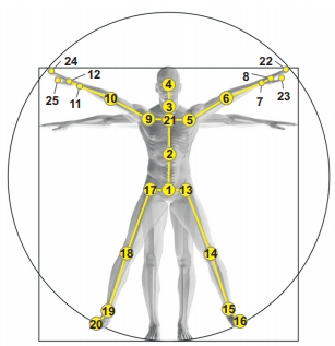
Figure 1: Illustration of body joints’ positions (only the first skeleton is shown). The joint at the hip is selected as the root of the skeleton. The distance between joints 1 and 6 is 4. The joints 22,23,24,25 are not used in the convolution operation. The arms then contain the following joints: $5,6,7,8,9,10,11,12$. The legs contain the following joints: $13,14,15,16,17,18,19,20$ (figure reproduced from [52]).

Here, the set of weights $\{\mathbf{W}_{u,v}\},u,v=1,2,3$ completely defines the convolution filters in Eq. (18). Let $N^{j,1}$ and $N^{j,2}$ be the numbers of joints belonging to the arms and legs of two skeletons, respectively (see Fig. 1). Let $\mathbf{X}^{out,1}$ and $\mathbf{X}^{out,2}$ respectively of size $N^{j,1}\times N^{f}\times d$ and $N^{j,2}\times N^{f}\times d$ be the data associated with the arms and legs of two persons. The motivation behind this partition is that the interaction between two persons often involve those among their arms and those among their legs. For each $b\in\{1,2\}$, the set of $N^{j,b}N^{f}$ $d-$dim feature vectors from $\mathbf{X}^{out,b}$ is partitioned into $L$ subsets using K-means clustering. Let $\mathbf{y}^{b}_{l,1},\ldots,\mathbf{y}^{b}_{l,i^{b}_{l}}$ be the feature vectors in the $l^{th}$ subset. We assume that $\mathbf{y}^{b}_{l,1},\ldots,\mathbf{y}^{b}_{l,i^{b}_{l}}$ are i.i.d. samples from a Gaussian $(\boldsymbol{\Sigma}^{b}_{l},\boldsymbol{\mu}^{b}_{l})$ whose parameters can be estimated as:

$$\boldsymbol{\mu}^{b}_{l}=\frac{1}{i^{b}_{l}}\sum_{j=1}^{i^{b}_{l}}\mathbf{y}^{b}_{l,j},$$ (20)

$$\boldsymbol{\Sigma}^{b}_{l}=\frac{1}{i^{b}_{l}-1}\sum_{j=1}^{i^{b}_{l}}(\mathbf{y}^{b}_{l,j}-\boldsymbol{\mu}^{b}_{l})(\mathbf{y}^{b}_{l,j}-\boldsymbol{\mu}_{l}^{b})^{T}.$$ (21)

Based on the theory developed in Section 4.1, the Gaussian $(\boldsymbol{\Sigma}^{b}_{l},\boldsymbol{\mu}^{b}_{l})$ can be identified with the following matrix:

$$\mathbf{P}^{b}_{l}=(\det\boldsymbol{\Sigma}_{l}^{b})^{-\frac{1}{n+k}}\begin{bmatrix}\boldsymbol{\Sigma}^{b}_{l}+k\boldsymbol{\mu}^{b}_{l}(\boldsymbol{\mu}_{l}^{b})^{T}&\boldsymbol{\mu}^{b}_{l}(k)\\ (\boldsymbol{\mu}_{l}^{b}(k))^{T}&\mathbf{I}_{k}\end{bmatrix}.$$ (22)

The above computations can be performed by a layer as:

$$\{\mathbf{P}^{b}_{l}\}^{b=1,2}_{l=1,\ldots,L}=f_{gaussemb}(\{\mathbf{X}^{out,b}\}_{b=1,2}).$$ (23)

The next layer is designed to compute statistics on SPD manifolds and can be written by:

$$\{\mathbf{P}^{b,m},\mathbf{P}^{b,c}\}_{b=1,2}=f_{spdstats}\big{(}\{\mathbf{P}^{b}_{l},\mathbf{W}^{b}_{pt}\}^{b=1,2}_{l=1,\ldots,L}\big{)},$$ (24)

where $\mathbf{W}^{b}_{pt},b=1,2$ are the parameters corresponding to the target points of PT (see Section 4.2). Specifically, $\mathbf{P}^{b,m}$ is the mean of $\mathbf{P}^{b}_{l},l=1,\ldots,L$, and $\mathbf{P}^{b,c}$ is given by:

$$\begin{split}\mathbf{P}^{b,c}=\frac{1}{L-1}\sum_{i=1}^{L}&f_{v}\big{(}\mathcal{T}_{\mathbf{P}^{b,m},\mathbf{W}^{b}_{pt}}(\overrightarrow{\mathbf{P}^{b,m}\mathbf{P}_{i}})\big{)}\times\\ &f_{v}\big{(}\mathcal{T}_{\mathbf{P}^{b,m},\mathbf{W}^{b}_{pt}}(\overrightarrow{\mathbf{P}^{b,m}\mathbf{P}_{i}})\big{)}^{T}.\end{split}$$ (25)

The next layer computes the embeddings of statistics $\mathbf{P}^{b,m},\mathbf{P}^{b,c},b=1,2$ and can be written as:

$$\{\mathbf{B}^{b}\}_{b=1,2}=f_{spdstatsemb}\big{(}\{\mathbf{P}^{b,m},\mathbf{P}^{b,c}\}_{b=1,2}\big{)},$$ (26)

where $\mathbf{B}^{b}$ is the embedding matrix of $(\mathbf{P}^{b,m},\mathbf{P}^{b,c})$ given in the right-hand side of (16).

The next layer transforms $\mathbf{B}^{b},b=1,2$ to some matrices in $LT^{+}(n^{\prime}+k^{\prime})$ as:

$$\{\mathbf{D}^{b}\}_{b=1,2}=f_{trilmap}\big{(}\{\mathbf{B}^{b},\mathbf{W}^{b}_{lw}\}_{b=1,2}\big{)},$$ (27)

where $\mathbf{D}^{b}=\mathbf{B}^{b}\mathbf{W}^{b}_{lw}$, $\mathbf{W}^{b}_{lw},b=1,2$ are the parameters that are required to be in $LT^{+}(n^{\prime}+k^{\prime})$ so that the outputs $\mathbf{D}^{b}$ are also in $LT^{+}(n^{\prime}+k^{\prime})$. The network then performs a projection:

$$\{\mathbf{E}^{b}\}_{b=1,2}=f_{triltoeud}(\{\mathbf{D}^{b}\}_{b=1,2}),$$ (28)

where $\mathbf{E}^{b}=f_{lm}(\mathbf{D}^{b}(\mathbf{D}^{b})^{T}),b=1,2$. Finally, a fully-connected (FC) layer and a softmax layer are used to obtain class probabilities:

$$\mathbf{C}^{out}=f_{prob}\big{(}concat(f_{v}(\mathbf{E}^{1}),f_{v}(\mathbf{E}^{2})),\mathbf{W}_{fc}\big{)},$$ (29)

where $\mathbf{W}_{fc}$ are the parameters of the FC layer, the operator $concat(\mathbf{V}_{1},\mathbf{V}_{2})$ concatenates the two column vectors $\mathbf{V}_{1}$ and $\mathbf{V}_{2}$ vertically, and $\mathbf{C}^{out}$ are the output class probabilities. We use the cross-entropy loss for training GeomNet.

4.5 Geometry Aware Constrained Optimization

Some layers of GeomNet rely on the eigenvalue decomposition. To derive the backpropagation updates for these layers, we follow the framework of [16] for computation of the involved partial derivatives. The optimization procedure for the parameters $\mathbf{W}^{b}_{pt},\mathbf{W}^{b}_{lw},b=1,2$ is based on the Adam algorithm in Riemannian manifolds [3]. The Riemannian Adam update rule is given by:

$$x_{t+1}=\exp_{x_{t}}\Bigg{(}-\alpha\frac{\hat{m}_{t}}{\sqrt{\hat{v}_{t}}+\epsilon}\Bigg{)},$$ (30)

where $x_{t}$ and $x_{t+1}$ are respectively the parameters updated at timesteps $t$ and $t+1$, $\hat{m}_{t}=m_{t}/(1-\beta_{1}^{t})$, $\hat{v}_{t}=v_{t}/(1-\beta_{2}^{t})$, $m_{t}=\beta_{1}\tau_{t-1}+(1-\beta_{1})g_{t}$ is a momentum term, $v_{t}=\beta_{2}v_{t-1}+(1-\beta_{2})\|g_{t}\|^{2}_{x_{t}}$ is an adaptivity term, $g_{t}$ is the gradient evaluated at timestep $t$, $\alpha,\epsilon,\beta_{1},\beta_{2}$ are constant values. The squared Riemannian norm $\|g_{t}\|^{2}_{x_{t}}=<g_{t}|g_{t}>_{x_{t}}$ corresponds to the squared gradient value in Riemannian settings. Here, $<.|.>_{x_{t}}$ is the dot product for the Riemannian metric of the manifold in consideration, as discussed in Section 3.1. After updating $x_{t+1}$ in Eq. (30), we update $\tau_{t}$ as the PT of $m_{t}$ along geodesics connecting $x_{t}$ and $x_{t+1}$, i.e. $\tau_{t}=\mathcal{T}_{x_{t},x_{t+1}}(m_{t})$.

The update rule in Eq. (30) requires the computation of the exponential map and the PT. For SPD manifolds, these operations are given in Eqs. (5) and (9). It remains to define these operations for the update of the parameters $\mathbf{W}^{b}_{lw},b=1,2$. To this aim, we rely on the Riemannian geometry of $LT^{+}(n)$ studied in the recent work [26]. By considering the following metric:

$$<\mathbf{U},\mathbf{V}>_{\mathbf{K}}=\sum_{i>j}\mathbf{U}_{ij}\mathbf{V}_{ij}+\sum_{j=1}^{n}\mathbf{U}_{jj}\mathbf{V}_{jj}\mathbf{K}_{jj}^{-2},$$ (31)

where $\mathbf{K}\in LT^{+}(n)$, $\mathbf{U},\mathbf{V}\in T_{\mathbf{K}}LT^{+}(n)$, $\mathbf{U}_{ij}$ is the element on the $i^{th}$ row and $j^{th}$ column of $\mathbf{U}$, Lin has shown [26] that the space $LT^{+}(n)$ (referred to as Cholesky space) equipped with the above metric forms a Riemannian manifold. On this manifold, the exponential map at a point can be computed as:

$$\exp_{\mathbf{K}}\mathbf{U}=\lfloor\mathbf{K}\rfloor+\lfloor\mathbf{U}\rfloor+\mathbb{D}(\mathbf{K})\exp(\mathbb{D}(\mathbf{U})\mathbb{D}(\mathbf{K})^{-1}),$$ (32)

where $\mathbf{K}\in LT^{+}(n)$, $\mathbf{U}\in T_{\mathbf{K}}LT^{+}(n)$, $\lfloor\mathbf{K}\rfloor$ is a matrix of the same size as $\mathbf{K}$ whose $(i,j)$ element is $\mathbf{K}_{ij}$ if $i>j$ and is zero otherwise, $\mathbb{D}(\mathbf{K})$ is a diagonal matrix whose $(i,i)$ element is $\mathbf{K}_{ii}$. Also, the PT of a tangent vector $\mathbf{U}\in T_{\mathbf{K}}LT^{+}(n)$ to a tangent vector at $\mathbf{H}\in LT^{+}(n)$ is given by:

$$\mathcal{T}_{\mathbf{K},\mathbf{H}}(\mathbf{U})=\lfloor\mathbf{U}\rfloor+\mathbb{D}(\mathbf{H})\mathbb{D}(\mathbf{K})^{-1}\mathbb{D}(\mathbf{U}),$$ (33)

where $\mathbf{K},\mathbf{H}\in LT^{+}(n)$.

5 Experiments

Our network was implemented with Tensorflow deep learning framework and the experiments were conducted using two NVIDIA GeForce GTX 1080 GPUs. We used GeomStats library [38] for geometric computations. The dimension $d$ of output vectors at the convolutional layer, the number of clusters $L$, and the learning rate were set to 9, 180, and $10^{-2}$, respectively. The batch sizes were set respectively to 30 and 256 for the experiments on SBU Interaction dataset and those on NTU datasets. The values of the pair $(k,k^{\prime})$ (see (3) and (16)) were set to $(2,3)$ and $(2,1)$ for the experiments on SBU Interaction and NTU datasets, respectively. The values of $\alpha,\epsilon,\beta_{1}$, and $\beta_{2}$ in the Riemannian Adam algorithm were set to $10^{-3},10^{-8},0.9$, and $0.999$, respectively [20]. In our experiments, GeomNet converged well after 600 epochs. For more details on our experiments, we refer the interested reader to the supplementary material.

5.1 Datasets and Experimental Settings

SBU Interaction dataset. This dataset [65] contains 282 sequences in 8 action classes created from 7 subjects. Each action is performed by two subjects where each subject has 15 joints. The joints 4,21,1,5,6,7,9,10,11,13,14,15,17,18,19 in Fig. 1 correspond respectively to the joints 1,2,3,4,5,6,7,8,9,10,11,12,13,14,15 of the first skeleton of SBU Interaction dataset. We followed the experimental protocol based on 5-fold cross validation with the provided training/testing splits [65].

NTU RGB+D 60 dataset. This dataset [52] contains 56,880 sequences created from 40 subjects with three cameras views and categorized into 60 classes. We followed the two experimental protocols cross-subject (X-subject) and cross-view (X-view) [52].

NTU RGB+D 120 dataset. This dataset [28] contains 114,480 sequences in 120 action classes, captured by 106 subjects with three cameras views. We followed the two experimental protocols cross-subject (X-subject) and cross-setup (X-setup) [28].

5.2 Ablation Study

In this section, we study the impact of different components of GeomNet on its accuracy on SBU Interaction and NTU RGB+D 60 datasets.

Embedding dimensions. Here we investigate the impact of the parameters $k$ and $k^{\prime}$ (see (3) and (16)). Fig. 2 shows the accuracies of GeomNet on SBU Interaction dataset with different settings of $(k,k^{\prime})$, i.e. $k=0,1,2$ and $k^{\prime}=0,\ldots,10$. Note that when $k=0$, the layer $f_{gaussemb}$ relies only on the covariance information. Also, when $k^{\prime}=0$, the outputs $\mathbf{B}^{b},b=1,2$ of the layer $f_{spdstatsemb}$ are simply obtained by the Cholesky decomposition of $\mathbf{P}^{b,c}$, i.e. $\mathbf{B}^{b}(\mathbf{B}^{b})^{T}=\mathbf{P}^{b,c}$. It is interesting to note that GeomNet achieves the best accuracy with $(k,k^{\prime})=(2,3)$, i.e. none of $k$ and $k^{\prime}$ is equal to 1. This is opposed to previous works [12, 25, 41, 59], where $n$-variate Gaussians are always identified with SPD $(n+1)\times(n+1)$ matrices. To the best of our knowledge, this is the first work that shows the benefits of identifying $n$-variate Gaussians with SPD $(n+k)\times(n+k)$ matrices where $k>1$. The results also reveal that the setting of $(k,k^{\prime})$ has a non-negligible impact on the accuracy of GeomNet. Namely, the performance gap between two settings $(k,k^{\prime})=(1,1)$ (94.54%) and $(k,k^{\prime})=(2,3)$ (96.33%) is 1.79%. We can also notice that when $k$ is fixed, GeomNet always performs best with $k^{\prime}>1$. This shows the effectiveness of our parameterization of Riemannian Gaussians in (16).

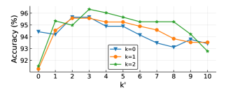
Figure 2: Accuracy of GeomNet on SBU Interaction dataset with different settings of $(k,k^{\prime})$.

Dataset	SBU Interaction	NTU RGB+D 60 Dataset
		X-Subject	X-View
Without PT	71.51	62.18	66.83
PT	96.33	93.62	96.32

Table 1: Effectiveness of PT on SBU Interaction and NTU RGB+D 60 datasets.

To investigate the effectiveness of our proposed embedding of Gaussians outside of our framework, we used it to improve the state-of-the-art neural network on SPD manifolds SPDNet [13]. In [13], the authors performed action recognition experiments by representing each sequence by a joint covariance descriptor. The covariance descriptor is computed from the second order statistics of the 3D coordinates of all body joints in each frame. For SBU Interaction dataset, the size of the covariance matrix is $90\times 90$ (30 body joints in each frame). In our experiment, we combined the covariance matrix and the mean vector using the proposed embedding of Gaussians to represent each sequence. Each sequence is then represented by a SPD $(90+k)\times(90+k)$ matrix. We used the code of SPDNet published by the authors. Fig. 3 shows the accuracies of SPDNet on SBU Interaction dataset with different settings of $k$. As can be observed, SPDNet gives the best accuracy with the setting $k=10$. The performance gap between two settings $k=1$ (90.5%) and $k=10$ (92.38%) is 1.88%. The accuracy of SPDNet when using only the covariance ($k=0$) is 79.48%, which is significantly worse than its accuracy with the setting $k=10$. The results confirm that our proposed embedding of Gaussians is effective in the framework of SPDNet and that it is advantageous over the one of [34]. This suggests that our method could also be beneficial to previous works that rely on Gaussians to capture local feature distribution, e.g. [12, 24, 25, 36, 41, 59].

Figure 3: Accuracy of SPDNet on SBU Interaction dataset with different settings of $k$.

Dataset	SBU Interaction	NTU RGB+D 60 Dataset
		X-Subject	X-View
Without LTML	94.90	92.30	95.05
LTML	96.33	93.62	96.32

Table 2: Effectiveness of lower triangular matrix learning (LTML) on SBU Interaction and NTU RGB+D 60 datasets.

Parallel transport. Tab. 1 gives the accuracies of GeomNet without using PT on SBU Interaction and NTU RGB+D 60 datasets. The accuracies of GeomNet are also shown for comparison purposes. When PT is not used, the covariance in Eq. (12) is computed as:

$$\mathbf{P}^{c}=\frac{1}{L-1}\sum_{i=1}^{L}f_{v}\big{(}\overrightarrow{\mathbf{P}^{m}\mathbf{P}_{i}}\big{)}f_{v}\big{(}\overrightarrow{\mathbf{P}^{m}\mathbf{P}_{i}}\big{)}^{T}.$$ (34)

It can be seen that the use of PT is crucial for obtaining high accuracy. Specifically, on NTU RGB+D 60 dataset, computing the covariance without PT results in a loss of 31.44% on X-Subject protocol and a loss of 29.49% on X-View protocol. On SBU Interaction dataset, a significant reduction in accuracy (24.82%) can also be observed when PT is not used. These results highlight the importance of learning the parameters $\mathbf{W}^{b}_{pt},b=1,2$ in GeomNet.

Lower triangular matrix learning. Tab. 2 gives the accuracies of GeomNet without using the layer $f_{trilmap}$ on SBU Interaction and NTU RGB+D 60 datasets. Again, the accuracies of GeomNet are also shown for comparison purposes. We can note that the introduction of the layer $f_{trilmap}$ brings performance improvement, i.e. 1.43% on SBU Interaction dataset, and 1.32% on X-Subject protocol and 1.27% on X-View protocol on NTU RGB+D 60 dataset.

5.3 Results on SBU Interaction Dataset

Results of GeomNet and state-of-the-art methods on SBU Interaction dataset are given in Tab. 3. For SPDNet, we report its best accuracy using the embedding in (3) with $k=10$. We can remark that the accuracies of most of the hand-crafted feature based methods [18, 56] are lower than 90%. The state-of-the-art method [9] for skeleton-based action recognition only gives a modest accuracy of 80.35%, the second worst accuracy among the competing methods. GeomNet achieves the best accuracy of 96.33%, which is 16.85% better than that of SPDNet.

Method	Accuracy
Lie Group [56]	47.92
Constrast Mining [18]	86.90
Interaction Graph [23]	92.56
Trust Gate LSTM [29]	93.30
Hierarchical RNN [9]	80.35
Deep LSTM+Co-occurence [68]	90.41
SPDNet [13]	92.38
GeomNet	96.33

Table 3: Recognition accuracy (%) of GeomNet and state-of-the-art methods on SBU Interaction dataset.

5.4 Results on NTU RGB+D 60 Dataset

Tab. 4 shows the results of GeomNet and state-of-the-art methods on NTU RGB+D 60 dataset. For ST-GCN and AS-GCN, we used the codes^, published by the authors. For SPDNet, we report its best accuracy using the embedding in (3) with $k=3$. We can observe that GeomNet gives the best results on this dataset. Since ST-GCN is based on fixed skeleton graphs which might miss implicit joint correlations, AS-GCN improves it by learning actional links to capture the latent dependencies between joints. AS-GCN also extends the skeleton graphs to represent structural links. However, AS-GCN does not achieve significant improvements over ST-GCN. This indicates that actional and structural links in AS-GCN are still not able to cope with complex patterns in 3DTPIR. As can be seen, GeomNet outperforms ST-GCN and AS-GCN by large margins. We can also note a large performance gap between GeomNet and SPDNet. This can probably be explained by the fact that: (1) GeomNet aims to learn inter-person joint relationships; (2) GeomNet leverages the covariance information on SPD manifolds.

Method	X-Subject	X-View
ST-LSTM [30]	83.0	87.3
ST-GCN [62]	86.75	91.17
AS-GCN [22]	87.08	92.04
LSTM-IRN [46]	90.5	93.5
SPDNet [13]	74.85	76.07
GeomNet	93.62	96.32

Table 4: Recognition accuracy (%) of GeomNet and state-of-the-art methods on NTU RGB+D 60 dataset.

Method	X-Subject	X-Setup
ST-LSTM [30]	63.0	66.6
ST-GCN [62]	78.60	79.92
AS-GCN [22]	77.83	79.30
LSTM-IRN [46]	77.7	79.6
ST-GCN-PAM [63]	83.28
SPDNet [13]	60.72	62.08
GeomNet	86.49	87.58

Table 5: Recognition accuracy (%) of GeomNet and state-of-the-art methods on NTU RGB+D 120 dataset.

5.5 Results on NTU RGB+D 120 Dataset

Results of GeomNet and state-of-the-art methods on NTU RGB+D 120 dataset are given in Tab. 5. For SPDNet, we report its best accuracy using the embedding in (3) with $k=3$. As can be observed, GeomNet performs best on this dataset. Note that LSTM-IRN performs significantly worse than GeomNet on this most challenging dataset. By adapting the graph structure in ST-GCN to involve connections between two skeletons, ST-GCN-PAM achieves significant improvements. However, ST-GCN-PAM is still outperformed by GeomNet by 3.21% on X-Subject protocol. The results indicate that: (1) without any prior knowledge, automatic inference of intra-person and inter-person joint relationships is difficult; (2) even with prior knowledge, the state-of-the-art ST-GCN performs worse than GeomNet. Compared to the results on NTU RGB+D 60 dataset, the performance gap between GeomNet and SPDNet is more pronounced on this dataset. Notice that our method is based only on the assumption that the joints of the arms of two persons and those of their legs are highly correlated during their interaction. Therefore, no explicit assumption in pairwise joint connections is required for interaction recognition.

6 Conclusion

We have presented GeomNet, a neural network based on embeddings of Gaussians and Riemannian Gaussians for 3DTPIR. To improve the accuracy of GeomNet, we have proposed the use of PT and a layer that learns lower triangular matrices with positive diagonal entries. Finally, we have provided experimental results on three benchmarks showing the effectiveness of GeomNet.

Acknowledgments. We thank the authors of NTU RGB+D datasets for providing access to their datasets.

References

- [1] Vincent Arsigny, Pierre Fillard, Xavier Pennec, and Nicholas Ayache. Fast and Simple Computations on Tensors with Log-Euclidean Metrics. Technical Report RR-5584, INRIA, 2005.
- [2] Frédéric Barbaresco. Jean-Louis Koszul and the Elementary Structures of Information Geometry. In Frank Nielsen, editor, Geometric Structures of Information, pages 333–392. Springer International Publishing, Cham, 2019.
- [3] Gary Bécigneul and Octavian-Eugen Ganea. Riemannian Adaptive Optimization Methods. In ICLR, 2019.
- [4] Daniel A. Brooks, Olivier Schwander, Frédéric Barbaresco, Jean-Yves Schneider, and Matthieu Cord. Riemannian Batch Normalization for SPD Neural Networks. In NeurIPS, pages 15463–15474, 2019.
- [5] Miquel Calvo and Josep M. Oller. A Distance between Multivariate Normal Distributions Based in an Embedding into the Siegel Group. Journal of Multivariate Analysis, 35(2):223–242, 1990.
- [6] Rudrasis Chakraborty and Baba Vemuri. Statistics on the (compact) Stiefel manifold: Theory and Applications. CoRR, abs/1708.00045, 2017.
- [7] Ke Cheng, Yifan Zhang, Xiangyu He, Weihan Chen, Jian Cheng, and Hanqing Lu. Skeleton-Based Action Recognition With Shift Graph Convolutional Network. In CVPR, pages 180–189, 2020.
- [8] Andrzej Cichocki and Shun-ichi Amari. Families of Alpha- Beta- and Gamma- Divergences: Flexible and Robust Measures of Similarities. Entropy, 12(6):1532–1568, 2010.
- [9] Yong Du, Wei Wang, and Liang Wang. Hierarchical Recurrent Neural Network for Skeleton Based Action Recognition. In CVPR, pages 1110–1118, 2015.
- [10] G. Evangelidis, G. Singh, and R. Horaud. Skeletal Quads: Human Action Recognition Using Joint Quadruples. In ICPR, pages 4513–4518, 2014.
- [11] R. Ferreira, J. Xavier, J. P. Costeira, and V. Barroso. Newton Method for Riemannian Centroid Computation in Naturally Reductive Homogeneous Spaces. In ICASSP, pages 704–707, 2006.
- [12] Liyu Gong, Tianjiang Wang, and Fang Liu. Shape of Gaussians as Feature Descriptors. In CVPR, pages 2366–2371, June 2009.
- [13] Zhiwu Huang and Luc Van Gool. A Riemannian Network for SPD Matrix Learning. In AAAI, pages 2036–2042, 2017.
- [14] Zhiwu Huang, Chengde Wan, Thomas Probst, and Luc Van Gool. Deep Learning on Lie Groups for Skeleton-Based Action Recognition. In CVPR, pages 6099–6108, 2017.
- [15] Zhiwu Huang, Jiqing Wu, and Luc Van Gool. Building Deep Networks on Grassmann Manifolds. In AAAI, pages 3279–3286, 2018.
- [16] Catalin Ionescu, Orestis Vantzos, and Cristian Sminchisescu. Matrix Backpropagation for Deep Networks with Structured Layers. In ICCV, pages 2965–2973, 2015.
- [17] Yanli Ji, Hong Cheng, Yali Zheng, and Haoxin Li. Learning Contrastive Feature Distribution Model for Interaction Recognition. Journal of Visual Communication and Image Representation, 33(C):340–349, 2015.
- [18] Yanli Ji, Guo Ye, and Hong Cheng. Interactive Body Part Contrast Mining for Human Interaction Recognition. In 2014 IEEE International Conference on Multimedia and Expo Workshops (ICMEW), pages 1–6, 2014.
- [19] Qiuhong Ke, Mohammed Bennamoun, Senjian An, Ferdous Sohel, and Farid Boussaïd. A New Representation of Skeleton Sequences for 3D Action Recognition. In CVPR, pages 4570–4579, 2017.
- [20] Diederik P. Kingma and Jimmy Ba. Adam: A Method for Stochastic Optimization. In ICLR, 2015.
- [21] Chaolong Li, Zhen Cui, Wenming Zheng, Chunyan Xu, and Jian Yang. Spatio-Temporal Graph Convolution for Skeleton Based Action Recognition. In AAAI, pages 3482–3489, 2018.
- [22] Maosen Li, Siheng Chen, Xu Chen, Ya Zhang, Yanfeng Wang, and Qi Tian. Actional-Structural Graph Convolutional Networks for Skeleton-Based Action Recognition. In CVPR, pages 3595–3603, 2019.
- [23] Meng Li and Howard Leung. Multiview Skeletal Interaction Recognition Using Active Joint Interaction Graph. IEEE Transactions on Multimedia, 18(11):2293–2302, 2016.
- [24] Peihua Li, Qilong Wang, Hui Zeng, and Lei Zhang. Local Log-Euclidean Multivariate Gaussian Descriptor and Its Application to Image Classification. TPAMI, 39(4):803–817, 2017.
- [25] P. Li, J. Xie, Q. Wang, and W. Zuo. Is Second-order Information Helpful for Large-scale Visual Recognition? In ICCV, pages 2070–2078, 2017.
- [26] Zhenhua Lin. Riemannian Geometry of Symmetric Positive Definite Matrices via Cholesky Decomposition. SIAM Journal on Matrix Analysis and Applications, 40(4):1353–1370, 2019.
- [27] Bangli Liu, Zhaojie Ju, and Honghai Liu. A Structured Multi-Feature Representation for Recognizing Human Action and Interaction. Neurocomputing, 318:287–296, 2018.
- [28] Jun Liu, Amir Shahroudy, Mauricio Perez, Gang Wang, Ling-Yu Duan, and Alex C. Kot. NTU RGB+D 120: A Large-Scale Benchmark for 3D Human Activity Understanding. TPAMI, 42(10):2684–2701, 2019.
- [29] J. Liu, A. Shahroudy, D. Xu, A. Kot Chichung, and G. Wang. Skeleton-Based Action Recognition Using Spatio-Temporal LSTM Network with Trust Gates. TPAMI, 40(12):3007–3021, 2018.
- [30] Jun Liu, Amir Shahroudy, Dong Xu, and Gang Wang. Spatio-Temporal LSTM with Trust Gates for 3D Human Action Recognition. In ECCV, pages 816–833, 2016.
- [31] Jun Liu, Gang Wang, Ping Hu, Ling-Yu Duan, and Alex C. Kot. Global Context-Aware Attention LSTM Networks for 3D Action Recognition. In CVPR, pages 3671–3680, 2017.
- [32] Mengyuan Liu, Hong Liu, and Chen Chen. Enhanced Skeleton Visualization for View Invariant Human Action Recognition. Pattern Recognition, 68:346–362, 2017.
- [33] Mengyuan Liu and Junsong Yuan. Recognizing Human Actions as The Evolution of Pose Estimation Maps. In CVPR, pages 1159–1168, 2018.
- [34] Miroslav Lovrić, Maung Min-Oo, and Ernst A Ruh. Multivariate Normal Distributions Parametrized As a Riemannian Symmetric Space. Journal of Multivariate Analysis, 74(1):36–48, 2000.
- [35] Jiajia Luo, Wei Wang, and Hairong Qi. Group Sparsity and Geometry Constrained Dictionary Learning for Action Recognition from Depth Maps. In ICCV, pages 1809–1816, 2013.
- [36] T. Matsukawa, T. Okabe, E. Suzuki, and Y. Sato. Hierarchical Gaussian Descriptor for Person Re-identification. In CVPR, pages 1363–1372, 2016.
- [37] Qianhui Men, Edmond S. L. Ho, Hubert P. H. Shum, and Howard Leung. A Two-Stream Recurrent Network for Skeleton-based Human Interaction Recognition. In ICPR, 2020.
- [38] Nina Miolane, Johan Mathe, Claire Donnat, Mikael Jorda, and Xavier Pennec. geomstats: a Python Package for Riemannian Geometry in Machine Learning. CoRR, abs/1805.08308, 2018.
- [39] Maher Moakher. A Differential Geometric Approach to the Geometric Mean of Symmetric Positive-definite Matrices. SIAM J. Matrix Anal. Appl., 26(3):735–747, 2005.
- [40] Juan C. Nez, Ral Cabido, Juan J. Pantrigo, Antonio S. Montemayor, and Jos F. Vlez. Convolutional Neural Networks and Long Short-Term Memory for Skeleton-based Human Activity and Hand Gesture Recognition. Pattern Recognition, 76(C):80–94, 2018.
- [41] Xuan Son Nguyen, Luc Brun, Olivier Lézoray, and Sébastien Bougleux. A Neural Network Based on SPD Manifold Learning for Skeleton-based Hand Gesture Recognition. In CVPR, pages 12036–12045, 2019.
- [42] Ouiza Ouyed and Mohand Said Allili. Group-of-features Relevance in Multinomial Kernel Logistic Regression and Application to Human Interaction Recognition. Expert Systems with Applications, 148:113247, 2020.
- [43] Xavier Pennec. Probabilities and Statistics on Riemannian Manifolds : A Geometric approach. Technical Report RR-5093, INRIA, 2004.
- [44] Xavier Pennec. Statistical Computing on Manifolds for Computational Anatomy. Habilitation à diriger des recherches, Université Nice Sophia-Antipolis, 2006.
- [45] Xavier Pennec, Pierre Fillard, and Nicholas Ayache. A Riemannian Framework for Tensor Computing. Technical Report RR-5255, INRIA, 2004.
- [46] Mauricio Perez, Jun Liu, and Alex C. Kot. Interaction Relational Network for Mutual Action Recognition. CoRR, abs/1910.04963, 2019.
- [47] C. Radhakrishna Rao. Information and the Accuracy Attainable in the Estimation of Statistical Parameters. In Samuel Kotz and Norman L. Johnson, editors, Breakthroughs in Statistics: Foundations and Basic Theory, pages 235–247. Springer New York, New York, NY, 1992.
- [48] Bin Ren, Mengyuan Liu, Runwei Ding, and Hong Liu. A Survey on 3D Skeleton-Based Action Recognition Using Learning Method. CoRR, abs/2002.05907, 2020.
- [49] Salem Said, Lionel Bombrun, Yannick Berthoumieu, and Jonathan Manton. Riemannian Gaussian Distributions on the Space of Symmetric Positive Definite Matrices. IEEE Trans. Inf. Theor., 63(4):2153–2170, 2017.
- [50] Salem Said, Hatem Hajri, Lionel Bombrun, and Baba C. Vemuri. Gaussian Distributions on Riemannian Symmetric Spaces: Statistical Learning With Structured Covariance Matrices. IEEE Trans. Inf. Theor., 64(2):752–772, 2018.
- [51] Adam Santoro, David Raposo, David G Barrett, Mateusz Malinowski, Razvan Pascanu, Peter Battaglia, and Timothy Lillicrap. A Simple Neural Network Module for Relational Reasoning. In NIPS, pages 4967–4976, 2017.
- [52] Amir Shahroudy, Jun Liu, Tian-Tsong Ng, and Gang Wang. NTU RGB+D: A Large Scale Dataset for 3D Human Activity Analysis. In CVPR, pages 1010–1019, 2016.
- [53] Chenyang Si, Wentao Chen, Wei Wang, Liang Wang, and Tieniu Tan. An Attention Enhanced Graph Convolutional LSTM Network for Skeleton-Based Action Recognition. In CVPR, pages 1227–1236, 2019.
- [54] Q. De Smedt, H. Wannous, and J. Vandeborre. Skeleton-Based Dynamic Hand Gesture Recognition. In CVPRW, pages 1206–1214, 2016.
- [55] Suvrit Sra and Reshad Hosseini. Conic Geometric Optimization on the Manifold of Positive Definite Matrices. SIAM Journal on Optimization, 25(1):713–739, 2015.
- [56] Raviteja Vemulapalli, Felipe Arrate, and Rama Chellappa. Human Action Recognition by Representing 3D Skeletons as Points in a Lie Group. In CVPR, pages 588–595, 2014.
- [57] Hongsong Wang and Liang Wang. Modeling Temporal Dynamics and Spatial Configurations of Actions Using Two-Stream Recurrent Neural Networks. CVPR, pages 3633–3642, 2017.
- [58] Jiang Wang, Zicheng Liu, Ying Wu, and Junsong Yuan. Mining Actionlet Ensemble for Action Recognition with Depth Cameras. In CVPR, pages 1290–1297, 2012.
- [59] Q. Wang, P. Li, and L. Zhang. G2DeNet: Global Gaussian Distribution Embedding Network and Its Application to Visual Recognition. In CVPR, pages 2730–2739, 2017.
- [60] J. Weng, M. Liu, X. Jiang, and J. Yuan. Deformable Pose Traversal Convolution for 3D Action and Gesture Recognition. In ECCV, pages 142–157, 2018.
- [61] Or Yair, Mirela Ben-Chen, and Ronen Talmon. Parallel Transport on the Cone Manifold of SPD Matrices for Domain Adaptation. IEEE Transactions on Signal Processing, 67(7):1797–1811, 2019.
- [62] Sijie Yan, Yuanjun Xiong, and Dahua Lin. Spatial Temporal Graph Convolutional Networks for Skeleton-Based Action Recognition. In AAAI, pages 7444–7452, 2018.
- [63] Chao-Lung Yang, Aji Setyoko, Hendrik Tampubolon, and Kai-Lung Hua. Pairwise Adjacency Matrix on Spatial Temporal Graph Convolution Network for Skeleton-Based Two-Person Interaction Recognition. In ICIP, pages 2166–2170, 2020.
- [64] Xiaodong Yang and Ying Li Tian. EigenJoints-based Action Recognition Using Naive-Bayes-Nearest-Neighbor. In CVPRW, pages 14–19, 2012.
- [65] K. Yun, J. Honorio, D. Chattopadhyay, T. L. Berg, and D. Samaras. Two-person Interaction Detection Using Body-pose Features And Multiple Instance Learning. In CVPRW, pages 28–35, 2012.
- [66] Miaomiao Zhang and P. Thomas Fletcher. Probabilistic Principal Geodesic Analysis. In NIPS, pages 1178–1186, 2013.
- [67] Xikang Zhang, Yin Wang, Mengran Gou, Mario Sznaier, and Octavia Camps. Efficient Temporal Sequence Comparison and Classification Using Gram Matrix Embeddings on a Riemannian Manifold. In CVPR, pages 4498–4507, 2016.
- [68] Wentao Zhu, Cuiling Lan, Junliang Xing, Wenjun Zeng, Yanghao Li, Li Shen, and Xiaohui Xie. Co-occurrence Feature Learning for Skeleton Based Action Recognition Using Regularized Deep LSTM Networks. In AAAI, pages 3697–3703, 2016.