Learning dynamical systems from data:
A simple cross-validation perspective,
part III: Irregularly-Sampled Time Series

Abstract.

A simple and interpretable way to learn a dynamical system from data is to interpolate its vector-field with a kernel. In particular, this strategy is highly efficient (both in terms of accuracy and complexity) when the kernel is data-adapted using Kernel Flows (KF) [34] (which uses gradient-based optimization to learn a kernel based on the premise that a kernel is good if there is no significant loss in accuracy if half of the data is used for interpolation). Despite its previous successes, this strategy (based on interpolating the vector field driving the dynamical system) breaks down when the observed time series is not regularly sampled in time. In this work, we propose to address this problem by directly approximating the vector field of the dynamical system by incorporating time differences between observations in the (KF) data-adapted kernels. We compare our approach with the classical one over different benchmark dynamical systems and show that it significantly improves the forecasting accuracy while remaining simple, fast, and robust.

1. Introduction

The ubiquity of time series in many domains of science has led to the development of diverse statistical and machine learning forecasting methods. Examples include ARIMA [10], GARCH [5] or LSTM [39]. Most of these methods require the time series to be regularly sampled in time. Yet, this requirement is not met in many applications. Indeed, irregularly sampled time series commonly arise in healthcare [29], finance [16] and physics [40] among other fields.

While adaptations have been proposed, these workarounds tend to consider the irregular sampling issue as a missing values problem, leading to poor performance when the resulting missing rate is very high. Such approaches include (1) the imputation of the missing values (e.g. with exponential smoothing [23, 42] or with a Kalman filter [17]), and (2) fast Fourier transforms or Lomb-Scargle periodograms [16, 2]. This issue has motivated the development of several recent deep learning-based algorithms such as VS-GRU [27], GRU-ODE-Bayes [28, 15] or ODE-RNN [18].

Amongst various learning-based approaches, kernel-based methods hold potential for considerable advantages in terms of theoretical analysis, numerical implementation, regularization, guaranteed convergence, automatization, and interpretability [11, 32]. Indeed, reproducing kernel Hilbert spaces (RKHS) [14] have provided strong mathematical foundations for analyzing dynamical systems [6, 21, 19, 20, 4, 24, 25, 1, 26, 7, 8, 9] and surrogate modeling (we refer the reader to [38] for a survey). Yet, the accuracy of these emulators depends on the kernel, and the problem of selecting a good kernel has received less attention. Recently, the experiments by Hamzi and Owhadi [22] show that when the time series is regularly sampled, Kernel Flows (KF) [34] (an RKHS technique) can successfully reconstruct the dynamics of some prototypical chaotic dynamical systems. KFs have subsequently been applied to complex large-scale systems, including climate data [30, 41]. The nonparametric version of KFs has been extended to dynamical systems in [35]. A KFs version for SDEs can be found in [36].

Despite its recent successes, we show in this paper that this strategy (based on approximating the vector field of the dynamical system) cannot directly be applied to irregularly sampled time series. Instead, we propose a simple adaptation to the original method that allows to significantly improve forecasting performance when the sampling is irregular. The adaptation is to approximate the vector field and can be reduced to adding time delays in between observations to the delay embedding used to feed the method. We demonstrate the benefits of our approach on three prototypical chaotic dynamical systems: the Hénon map, the Van der Pol oscillator, and the Lorenz map. For all, our approach shows significantly improved forecasting accuracy (compared to the original approach).

Specifically, our contributions are as follows:

• We show that learning the kernel in kernel ridge regression using our modified approach significantly improves the prediction performance for irregular time series of dynamical systems

• Using a delay embedding, we adapt the KF-adapted kernel method algorithm to make multistep predictions

The outline of this paper is as follows. In Section 2, we review kernel methods for regularly sampled time series and propose an extension of Kernel Flows to irregularly sampled time series. Section 3 contains a description of our experiments with the Hénon, Van der Pol, and Lorenz systems and a discussion. The appendix provides a summary of the theory of reproducing kernel Hilbert spaces (RKHS).

2. Statement of the problem and proposed solution

2.1. The problem

Let $x_{1},x_{2},...,x_{n}$ be observations from a deterministic dynamical system in $\mathbb{R}^{d}$, along with a vector $t=(t_{1},\ldots,t_{n})$ containing the time of observations. That is, the observation $x_{k}$ is observed at time $t_{k}$. Importantly, time differences in between observation $t_{k+1}-t_{k}$ are not necessarily regular. Our goal is to predict $x_{n+1},x_{n+2},\ldots$ given the future sampling times $t_{n+1},t_{n+2},...$ and the history of the irregularly observed time series ($x_{1},...x_{n}$ and $t_{1},...,t_{n}$).

2.2. A reminder on kernel methods for regularly sampled time series

The simplest approach to forecasting the time series (employed in [22]) is to assume that $x_{1},x_{2},\ldots$ is the solution of a discrete dynamical system of the form

$$x_{k+1}=f^{\dagger}(x_{k},\ldots,x_{k-\tau^{\dagger}+1}),$$ (1)

with an unknown vector field $f^{\dagger}$ and time delay $\tau\in\mathbb{N}^{*}$ (which we will call delay or delay embedding) and approximate $f^{\dagger}$ with a kernel interpolant $f$ of the past data (a kernel ridge regression model [13]) and use the resulting surrogate model $x_{k+1}=f(x_{k},\ldots,x_{k-\tau^{\dagger}+1})$ to predict future state.

Given $\tau\in\mathbb{N}^{*}$ (see [22] for how $\tau$ can be learned in practice), the approximation of the dynamical system can then be recast as that of interpolating $f^{\dagger}$ from pointwise measurements

$$f^{\dagger}(X_{k})=Y_{k}\text{ for }k=1,\ldots,N,$$ (2)

with $X_{k}:=(x_{k},\ldots,x_{k+\tau-1})$, $Y_{k}:=x_{k+1}$ and $N=n-\tau$. Given a reproducing kernel Hilbert space of candidates $\mathcal{H}$ for $f^{\dagger}$, and using the relative error in the RKHS norm $\|\cdot\|_{\mathcal{H}}$ as a loss, the regression of the data $(X_{k},Y_{k})$ with the kernel $K$ associated with $\mathcal{H}$ provides a minimax optimal approximation [33] of $f^{\dagger}$ in $\mathcal{H}$. This regressor (in the presence of measurement noise of variance $\lambda>0$) is

$$f(x)=K(x,X)(K(X,X)+\lambda I)^{-1}Y,$$ (3)

where $X=(X_{1},\ldots,X_{N})$, $Y=(Y_{1},\ldots,Y_{N})$, $k(X,X)$ is the $N\times N$ matrix with entries $k(X_{i},X_{j})$, $k(x,X)$ is the $N$ vector with entries $k(x,X_{i})$ and $I$ is the identity matrix. This regressor has also a natural interpretation in the setting of Gaussian process (GP) regression: (i.) (3) is the conditional mean of the centered GP $\xi\sim\mathcal{N}(0,K)$ with covariance function $K$ conditioned on $\xi(X_{k})+\sqrt{\lambda}Z_{k}=Y_{k}$ where the $Z_{k}$ are centered i.i.d. normal random variables of variance $\lambda$.

2.3. A reminder on the Kernel Flows (KF) algorithm

The accuracy of any kernel-based method depends on the kernel $K$, and [22] proposed (in the setting of Subsec. 2.2) to also learn that kernel from the data $(X_{k},Y_{k})$ with the Kernel Flows (KF) algorithm [34, 44, 12] which we will now recall.

To describe this algorithm, let $K_{\theta}(x,x^{\prime})$ be a family of kernels parameterized by $\theta$. Using the notations from Subsection 2.2, the interpolant of the data $(X,Y)$ ($X=(X_{1},\ldots,X_{N})$ and $Y=(Y_{1},\ldots,Y_{N})$) obtained with the kernel $K_{\theta}$ (and a nugget $\lambda>0$) admits the representer formula

$$u_{N}(x)=K_{\theta}(x,X)(K_{\theta}(X,X)+\lambda I)^{-1}Y$$ (4)

A fundamental question is then: which $\theta$ should be chosen in (4)? KF answers that question by learning $\theta$ from data based on the simple premise that a kernel ($K_{\theta}$) is good if the interpolant (4) does not change much under subsampling of the data. This simple cross-validation concept is then turned into an iterative algorithm as follows.
1. Given $M\leq N$, select a random subset $\{\pi_{1},\ldots,\pi_{M}\}$ of $\{1,\ldots,N\}$ and a random subset $\{\beta_{1},\ldots,\beta_{\frac{M}{2}}\}$ of $\{\pi_{1},\ldots,\pi_{M}\}$. Write $X^{\pi}$ and $Y^{\pi}$ for the sub-vectors $(X_{\pi_{1}},\ldots,X_{\pi_{M}})$ and $(Y_{\pi_{1}},\ldots,Y_{\pi_{M}})$. Write $X^{\beta}$ and $Y^{\beta}$ for the sub-vectors $(X_{\beta_{1}},\ldots,X_{\beta_{\frac{M}{2}}})$ and $(Y_{\beta_{1}},\ldots,Y_{\beta_{\frac{M}{2}}})$.
2. Write $u_{\pi}(x)=K_{\theta}(x,X^{\pi})(K(X^{\pi},X^{\pi})+\lambda I)^{-1}Y^{\pi}$ and $u_{\beta}(x)=K_{\theta}(x,X^{\beta})(K(X^{\beta},X^{\beta})+\lambda I)^{-1}Y^{\beta}$ for the regressors of $(X^{\pi},Y^{\pi})$ and $(X^{\beta},Y^{\beta})$ obtained with the kernel $K_{\theta}$.
3. Write

$$\rho(\theta):=1-\frac{Y^{\beta,T}(K_{\theta}(X^{\beta},X^{\beta})+\lambda I)^{-1}Y^{\beta}}{Y^{\pi,T}(K_{\theta}(X^{\pi},X^{\pi})+\lambda I)^{-1}Y^{\pi}}\,.$$ (5)

Note that (a) when $\lambda=0$ then $\rho(\theta)$ is the relative square error $\frac{||u_{\pi}-u_{\beta}||^{2}_{K_{\theta}}}{||u_{\pi}||^{2}_{K_{\theta}}}$ between the interpolants $u_{\pi}$ and $u_{\beta}$, (b) when $\lambda\geq 0$ then $\rho(\theta)$ is the relative difference $1-\frac{\|u_{\beta}||^{2}_{K_{\theta}}+\lambda^{-1}|u_{\beta}(X^{\beta})-Y^{\beta}|^{2}}{||u_{\pi}||^{2}_{K_{\theta}}+\lambda^{-1}|u_{\pi}(X^{\pi})-Y^{\pi}|^{2}}$ between the regression losses (c) $\rho(\theta)$ lies between 0 and 1 inclusive.
4. Move $\theta$ in the gradient descent direction of $\rho$: $\theta\leftarrow\theta-\eta\nabla_{\theta}\rho$
5. Repeat until the error reaches a minimum.

2.4. The problem with irregularly sampled time series

The model (1) fails to be accurate for irregularly sampled series because it discards the information contained in the $t_{k}$. When the $x_{k}$ are obtained by sampling a continuous dynamical system, one could consider the following alternative model:

$$x_{k+1}=x_{k}+(t_{k+1}-t_{k})f^{\dagger}(x_{k}),$$ (6)

While this approach may succeed if the time intervals $t_{k+1}-t_{k}$ are small enough, it will also break down as these time intervals get larger. In our experiments section, we refer to this approach as the Euler approach, as it consists in learning the Euler discretization of the vector field.

2.5. The proposed solution

To address this issue, we consider the model

$$x_{k+1}=f^{\dagger}(x_{k},\Delta_{k},\ldots,x_{k-\tau^{\dagger}+1},\Delta_{k-\tau^{\dagger}+1}),$$ (7)

which incorporates the time differences $\Delta_{k}=t_{k+1}-t_{k}$ between observations. That is, we employ a time-aware time series representations by interleaving observations and time differences. The proposed strategy is then to construct a surrogate model of (7) by regressing $f^{\dagger}$ from past data and a kernel $K_{\theta}$ learned with Kernel Flows as described in Subsec. 2.3. Note that the past data takes the form (2) with $X_{k}:=(x_{k},\Delta_{k},\ldots,x_{k+\tau-1},\Delta_{k+\tau-1})$, $Y_{k}:=x_{k+1}$ and $N=n-\tau$.

3. Experiments

We conduct numerical experiments on three well-known dynamical systems: the Hénon map, the van der Pol oscillator, and the Lorenz map. We generate irregularly sampled time series from these dynamical systems using numerical integration and subsequently split the time series into training and test subsets. The time series are subsequently irregularly sampled according to the following scheme. The time interval between each observation $\Delta_{k}$ is taken to be a multiple of the smallest integration setup used to generate the data $\delta_{t}$. That is, $\Delta_{k}=\alpha_{k}\delta_{t}$ where $\alpha_{k}$ is a random integer between $1$ and $\alpha$. We train the kernel on the training part of the time series and evaluate the forecasting performance of the model. We report both the mean squared error (MSE) and the coefficient of determination ($R^{2}$).

Given test samples $x_{n+1},x_{n+2},...,x_{N}$ and the predictions $\hat{x}_{n+1},\hat{x}_{n+2},...,\hat{x}_{N}$, the MSE and the coefficient of determination are computed as follows:

$$MSE =\frac{1}{N-n}\sum_{i=n+1}^{N}||x_{i}-\hat{x}_{i}||_{2}^{2}$$

$$R^{2} =1-\frac{\sum_{i=n+1}^{N}||x_{i}-\hat{x}_{i}||_{2}^{2}}{\sum_{i=n+1}^{N}||x_{i}-\bar{x}||_{2}^{2}}.$$

where $\bar{x}=\frac{1}{N-n}\sum_{i=n+1}^{N}x_{i}$. The MSE should then be as low as possible and the $R^{2}$ as high as possible. We note that it is possible to have a negative $R^{2}$, if the predictor performs worse than the average of the samples.

To showcase the importance of learning the kernel parameters and to include the time difference between subsequent observations, we proceed in three stages. We first report the results of our method when the parameters of the kernel are not learned but rather sampled at random from a uniform ($\mathcal{U}(0,1)$) distribution and when the time delays are not encoded in the input data. In this setup, we distinguish the original KF case and the Euler version, as discussed in Subsection 2.4. Second, to assess the importance of learning the Kernel parameters, we report the model performance when the parameters are learned but the time delays are not encoded in the input data. Lastly, we report the performance of our approach when we both learned the kernel parameters and included the time delays.

For all models variants and dynamical systems, we use the training procedure as described in [22] and used a mini-batch size of 100 temporal observations and minimize $\rho(\theta)$ as in Equation 5 using stochastic gradient descent. To allow for a notion of uncertainty in the reported metrics, all our experiments use a five repetition approach where five different kernel initialization are randomly chosen.

In all of our examples, we used a kernel that is a linear combination of the triangular, Gaussian, Laplace, locally periodic kernels, and the quadratic kernel.

$$K(x,y)=\gamma^{2}_{0}\max(0,1-\frac{||x-y||^{2}_{2}}{\sigma_{0}^{2}})+\gamma^{2}_{1}e^{\frac{||x-y||^{2}_{1}}{\sigma^{2}_{1}}}+\gamma^{2}_{2}e^{\frac{-||x-y||_{2}}{\sigma^{2}_{2}}}+\gamma^{2}_{3}e^{-\sigma_{3}\sin^{2}(\sigma_{4}\pi||x-y||^{2}_{2})}e^{\frac{-||x-y||^{2}_{2}}{\sigma^{2}_{5}}}+\gamma^{2}_{4}||x-y||^{2}_{2}$$ (8)

Multi-step predictions:

By learning the dynamical systems of interest, we aim at delivering accurate forecasting predictions over the longest horizon possible. However, due to the chaotic nature of the studied dynamical systems, this horizon is intrinsically limited. To use most of the testing section of the time series, we then predict the future of the time series in chunks. That is, for a horizon $h$ and for a delay embedding with delay $d$, we split the test time series in chunks of lengths $h+d$. For each of these chunks, we use the $d$ first samples as input to our model and predict over the $h$ remaining samples in the chunk. We eventually aggregate the predictions of all samples overall chunks together to compute the reporting metrics.

Overview.

Recapping, we will compare 5 approaches:

1. Regressing model (7) with a kernel learnt using KF (which we call irregular KF).

2. Regressing model (1) with a kernel learned using KF (which we call regular KF).

3. Regressing model (6) with a kernel learned using KF (which we call the Euler version).

4. Regressing model (7) without learning the kernel.

5. Regressing model (1) without learning the kernel.

Table 1 summarizes results obtained in the following sections.

Table 1. Test performance of the different datasets. We report the means along with standard deviations of the mean squared error (MSE) and coefficient of determination ($R^{2}$) on the forecasting task. As Hénon is not a time-continuous map, the Euler version of KF is not applicable in this case. For readability, we abstain from reporting the exact numbers when MSE is larger than one and $R^{2}$ larger lower than 0.

Method	Hénon		Lorenz		Van der Pol
	MSE	$R^{2}$	MSE	$R^{2}$	MSE	$R^{2}$
(A) Kernel-IFlow	$0.024\pm 0.015$	$0.869\pm 0.081$	$0.003\pm 0.003$	$0.967\pm 0.029$	$0.001\pm 0.001$	$0.998\pm 0.002$
(B) KernelFlow	$0.190\pm 0.008$	$-0.050\pm 0.041$	$0.026\pm 0.015$	$0.700\pm 0.170$	$>>1$	$<<0$
(C) KernelFlow (Euler)	/	/	$0.005\pm 0.002$	$0.947\pm 0.023$	$>>1$	$<<0$
(D) - no learning	$>>1$	$<<0$	$>>1$	$<<0$	$>>1$	$<<0$
(E) - no learning	$>>1$	$<<0$	$>>1$	$<<0$	$>>1$	$<<0$

3.1. Hénon map

Consider the Hénon map with $a=1.4,b=0.3$

$$x_{n+1}=1-ax_{n}^{2}+y_{n},y_{n+1}=bx_{n}$$ (9)

We have repeated our experiments five times with a delay embedding of 1, a learning rate $\eta$ of 0.1, a prediction horizon $h$ of 5, maximum time difference $\alpha$ of 3, and have trained the model on 600 points to predict the next 400 points. Fig. 1i shows that approach (E) cannot reconstruct the attractor because it makes no attempt at learning the kernel and ignores time differences in the sampling. Fig. 1ii shows that embedding the time delay in the kernel (approach (A)) significantly improves the reconstruction of the attractor of the Hénon map. Table 1 displays the forecasting performance of the different methods. We observe that if the kernel is not learned (if the kernel is not data adapted), then the underlying method is unable to learn an accurate representation of the dynamical system. However, if the parameters of the kernel are learned, then our proposed approach (A) clearly outperforms the regular KF (approach (B)). As for the Euler version, it is not applicable in this case as Hénon is not a continuous map.

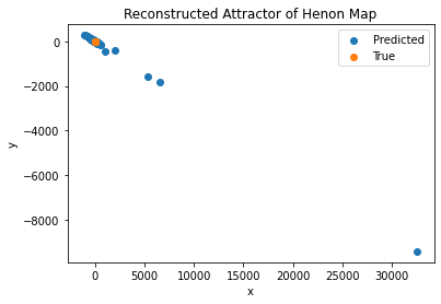
i Approach (E). Attractor Reconstruction by regressing model (1) without learning the kernel (horizon has been reduced to 1).

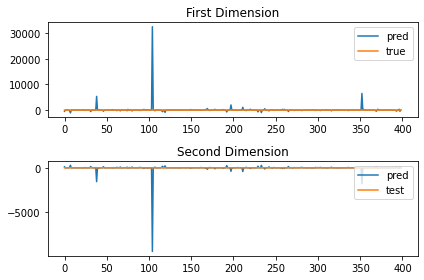
ii Approach (E). Time series reconstruction by regressing model (1) without learning the kernel (horizon has been reduced to 1).

Figure 1. Hénon map reconstructions when the kernel parameters are not learnt (regression of model (1) without learning the kernel).

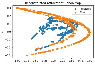
i Approach (B). With regular Kernel Flows (regression of model (1) with a kernel learnt using KF)

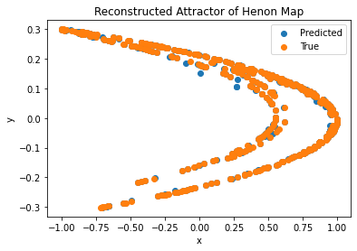
ii Approach (A). With irregular Kernel Flows (regression of model (7) with a kernel learnt using KF)

Figure 2. Hénon map attractor reconstructions with learnt kernels.

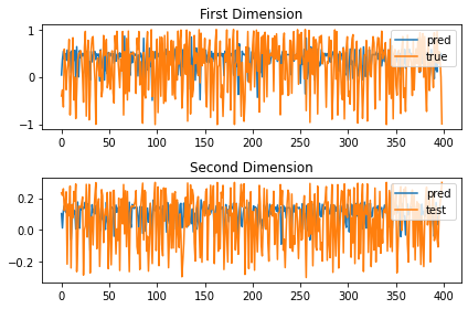
i Approach (B). With regular Kernel Flows

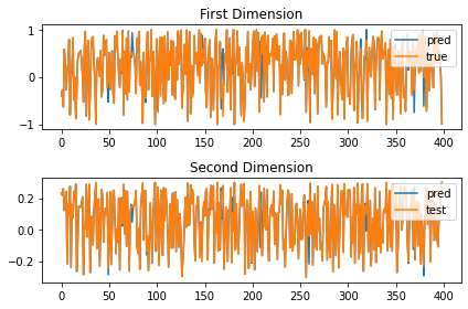
ii Approach (A). With irregular Kernel Flows

Figure 3. Reconstruction (prediction) of the test time series of the Hénon map.

3.2. Van der Pol oscillator

The second dynamical system of interest is the van der Pol oscillator represented by

$$\frac{dx}{dt}=\frac{1}{\epsilon}f(x,y)\ ,\ \frac{dy}{dt}=g(x,y)$$ (10)

where $f(x,y)=y-\frac{27}{4}x^{2}(x+1),\ g=-\frac{1}{2}-x\ ,\epsilon=0.01$.

Here, we have used a prediction horizon $h$ of 10, a learning rate $\eta$ of 0.01, a maximum time difference $\alpha$ of 5, and a delay embedding of 1. As evident from Table 1 and the following figures, our proposed approach (A) is the only one able to extract any meaningful representation of the dynamical system (including predicting future critical transitions). Other approaches are not accurate and/or exhibit forecasting instabilities.

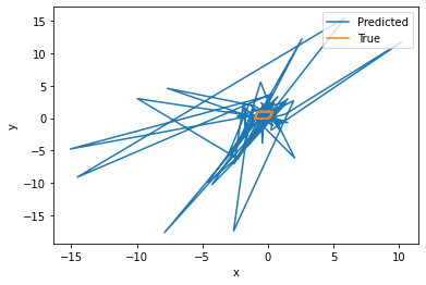
i Attractor Reconstruction.

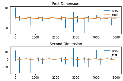
ii Time series reconstruction.

Figure 4. Van der Pol oscillator without learning the kernel (horizon has been reduced to 1).

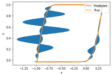
i Approach (B): with regular Kernel Flows (the horizon has been reduced to 4).

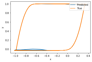
ii Approach (A): with irregular Kernel Flows

Figure 5. Van der Pol attractor reconstruction.

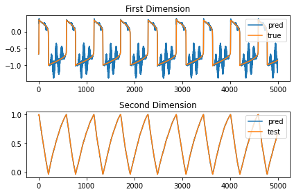
i Approach (B): with regular Kernel Flows

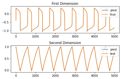
ii Approach (A): With irregular Kernel Flows

Figure 6. Reconstruction of the test time series of the Van der Pol oscillator with irregular and regular Kernel Flows.

3.3. Lorenz

Our third example is the Lorenz system described by the following system of differential equations:

$$\dot{x}=\sigma(y-x),\ \dot{y}=x(\rho-z)-y,\ \dot{z}=xy-\beta z\,,$$ (11)

with standard parameter values $\sigma=10,\ \rho=28\ ,\beta=\frac{8}{3}$

Our parameters include a delay embedding of 2, a learning rate $\eta=0.01$, a prediction horizon $h=20$, a maximum time difference $\alpha=5$, 5000 points used for training and the 5000 for testing. Fig. 7, 8 and 9 show that (1) not learning the kernel or not including time differences lead to poor reconstructions of the attractor of the Lorenz system even if the time horizon is 1. However, as observed in Table 1, the Euler version of KF leads to satisfying results, close to (but not as good as) the ones obtained with our proposed approach (A).

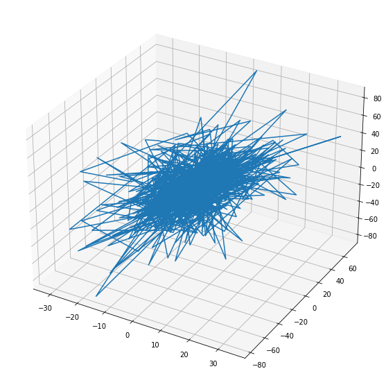
i Attractor reconstruction.

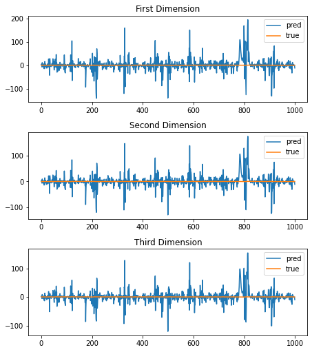
ii Time series reconstruction.

Figure 7. Lorenz map without learning the kernel (horizon has been reduced to 1).

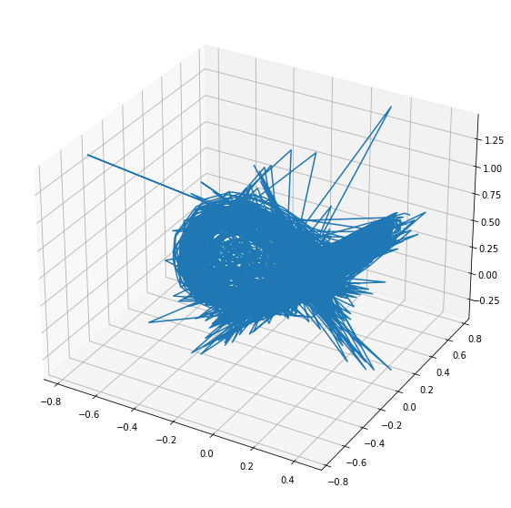
i Approach (B): With regular Kernel Flows

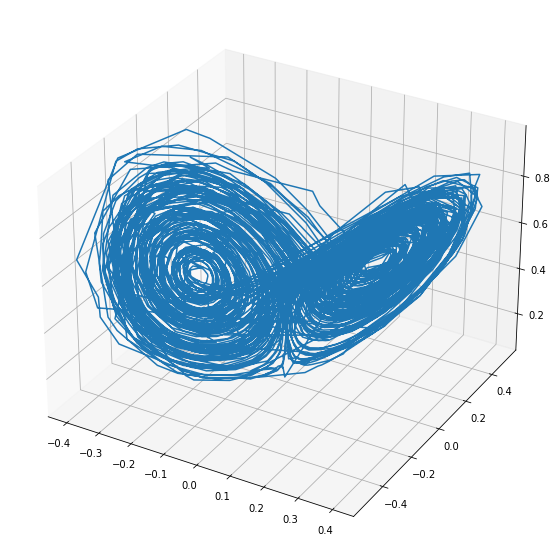
ii Approach (A): with irregular Kernel Flows

Figure 8. Lorenz map attractor reconstruction with learnt kernel.

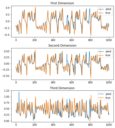
i Approach (B): with regular Kernel Flows

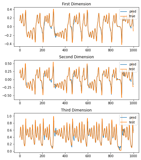
ii Approach (A): with irregular kernel flows

Figure 9. Reconstruction of the test time series of the Lorenz map with irregular and regular Kernel Flows.

Remark (Real-time learning and Newton basis):

It is possible to include new measurements when approximating the dynamics from data without repeating the learning process. This can be done by working in Newton basis as in [37] (see also section 4 of [38]). The Newton basis is just another basis for the space spanned by the kernel on the points, i.e., $\mbox{span}\{k(.,x_{1}),....,k(.,x_{N})\}=\mbox{span}\{v_{1},...,v_{N}\}$.

The kernel expansion of $f$ writes as $f(x)=\sum_{i=1}^{N}c_{i}K(x,x_{i})=\sum_{i=1}^{N}b_{i}v_{i}(x)$ with $<v_{i},v_{j}>_{H}=\delta_{ij}$ (i.e., the basis is orthonormal in the RKHS inner product).

If we add a new point $x_{N+1},...,x_{N+m}$, we’ll have corresponding elements $v_{N+1},...,v_{N+m}$ of the Newton basis, still orthonormal to the previous ones. So we will have a new interpolant $f_{\mbox{new}}(x)=\sum_{i=1}^{N+m}b_{i}v_{i}(x)$ that can be rewritten in terms of the old interpolant as

$$f_{\mbox{new}}(x)=\sum_{i=1}^{N+m}c_{i}v_{i}(x)=f(x)+\sum_{i=N+1}^{N+m}c_{i}v_{i}(x),$$

where $f$ can still be written in terms of the basis K, but with different coefficients $c^{\prime}$.

If $A$ is the kernel matrix on the first $N$ points, on can compute a Cholesky factorization $A=LL^{T}$ with $L$ lower triangular. Let $B:=L^{-T}$, then $v_{j}(x)=\sum_{i=1}^{N}(B)_{ij}K(x,x_{i})$.

When we add new points, we have an updated kernel matrix $A^{\prime}$, and the Cholesky factor of $A$ can be easily updated to the one of $A^{\prime}$.

4. Conclusion

Our numerical experiments demonstrate that embedding the time differences between the observations in the kernel considerably improves the forecasting accuracy with irregular time series. Though we have focused on a few examples, the success of our proposed approach (A) has raised the question of whether it can be extended to other systems, including those described by partial and stochastic differential equations, as well as complex real-world data.

5. Appendix

5.1. Reproducing Kernel Hilbert Spaces (RKHS)

We give a brief overview of reproducing kernel Hilbert spaces as used in statistical learning theory  [14]. Early work developing the theory of RKHS was undertaken by N. Aronszajn [3].

Definition 5.1.

Let ${\mathcal{H}}$ be a Hilbert space of functions on a set ${\mathcal{X}}$. Denote by $\langle f,g\rangle$ the inner product on ${\mathcal{H}}$ and let $\|f\|=\langle f,f\rangle^{1/2}$ be the norm in ${\mathcal{H}}$, for $f$ and $g\in{\mathcal{H}}$. We say that ${\mathcal{H}}$ is a reproducing kernel Hilbert space (RKHS) if there exists a function $K:{\mathcal{X}}\times{\mathcal{X}}\rightarrow\mathbb{R}$ such that
i. $K_{x}:=K(x,\cdot)\in{\mathcal{H}}$ for all $x\in{\mathcal{X}}$.
ii. $K$ spans ${\mathcal{H}}$: ${\mathcal{H}}=\overline{\mbox{span}\{K_{x}~{}|~{}x\in{\mathcal{X}}\}}$.
iii. $K$ has the reproducing property: $\forall f\in{\mathcal{H}}$, $f(x)=\langle f,K_{x}\rangle$.
$K$ will be called a reproducing kernel of ${\mathcal{H}}$. ${\mathcal{H}}_{K}$ will denote the RKHS ${\mathcal{H}}$ with reproducing kernel $K$ where it is convenient to explicitly note this dependence.

The important properties of reproducing kernels are summarized in the following proposition.

Proposition 5.1.

If $K$ is a reproducing kernel of a Hilbert space ${\mathcal{H}}$, then
i. $K(x,y)$ is unique.
ii. $\forall x,y\in{\mathcal{X}}$, $K(x,y)=K(y,x)$ (symmetry).
iii. $\sum_{i,j=1}^{q}\beta_{i}\beta_{j}K(x_{i},x_{j})\geq 0$ for $\beta_{i}\in\mathbb{R}$, $x_{i}\in{\mathcal{X}}$ and $q\in\mathbb{N}_{+}$ (positive definiteness).
iv. $\langle K(x,\cdot),K(y,\cdot)\rangle=K(x,y)$.

Common examples of reproducing kernels defined on a compact domain $\mathcal{X}\subset\mathrm{R}^{n}$ are the (1) constant kernel: $K(x,y)=k>0$ (2) linear kernel: $K(x,y)=x\cdot y$ (3) polynomial kernel: $K(x,y)=(1+x\cdot y)^{d}$ for $d\in\mathbb{N}_{+}$ (4) Laplace kernel: $K(x,y)=e^{-||x-y||_{2}/\sigma^{2}}$, with $\sigma>0$ (5) Gaussian kernel: $K(x,y)=e^{-||x-y||^{2}_{2}/\sigma^{2}}$, with $\sigma>0$ (6) triangular kernel: $K(x,y)=\max\{0,1-\frac{||x-y||_{2}^{2}}{\sigma}\}$, with $\sigma>0$. (7) locally periodic kernel: $K(x,y)=\sigma^{2}e^{-2\frac{\sin^{2}(\pi||x-y||_{2}/p)}{\ell^{2}}}e^{-\frac{||x-y||_{2}^{2}}{2\ell^{2}}}$, with $\sigma,\ell,p>0$.

Theorem 5.1.

Let $K:{\mathcal{X}}\times{\mathcal{X}}\rightarrow\mathbb{R}$ be a symmetric and positive definite function. Then there exists a Hilbert space of functions ${\mathcal{H}}$ defined on ${\mathcal{X}}$ admitting $K$ as a reproducing Kernel. Conversely, let ${\mathcal{H}}$ be a Hilbert space of functions $f:{\mathcal{X}}\rightarrow\mathbb{R}$ satisfying $\forall x\in{\mathcal{X}},\exists\kappa_{x}>0,$ such that $|f(x)|\leq\kappa_{x}\|f\|_{\mathcal{H}},\quad\forall f\in{\mathcal{H}}.$ Then ${\mathcal{H}}$ has a reproducing kernel $K$.

Theorem 5.2.

Let $K(x,y)$ be a positive definite kernel on a compact domain or a manifold $X$. Then there exists a Hilbert space $\mathcal{F}$ and a function $\Phi:X\rightarrow\mathcal{F}$ such that

$$K(x,y)=\langle\Phi(x),\Phi(y)\rangle_{\mathcal{F}}\quad\mbox{for}\quad x,y\in X.$$

$\Phi$ is called a feature map, and $\mathcal{F}$ a feature space.

5.2. Function Approximation in RKHSs: An Optimal Recovery Viewpoint

In this section, we review function approximation in RKHSs from the point of view of optimal recovery as discussed in [33].

Problem P:

Given input/output data $(x_{1},y_{1}),\cdots,(x_{N},y_{N})\in\mathcal{X}\times\mathbb{R}$, recover an unknown function $u^{\ast}$ mapping $\mathcal{X}$ to $\mathbb{R}$ such that $u^{\ast}(x_{i})=y_{i}$ for $i\in\{1,...,N\}$.

In the setting of optimal recovery, [33] Problem P can be turned into a well-posed problem by restricting candidates for $u$ to belong to a Banach space of functions $\mathcal{B}$ endowed with a norm $||\cdot||$ and identifying the optimal recovery as the minimizer of the relative error

$$\mbox{min}_{v}\mbox{max}_{u}\frac{||u-v||^{2}}{||u||^{2}},$$ (12)

where the max is taken over $u\in\mathcal{B}$ and the min is taken over candidates in $v\in\mathcal{B}$ such that $v(x_{i})=u(x_{i})=y_{i}$. For the validity of the constraints $u(x_{i})=y_{i}$, $\mathcal{B}^{\ast}$, the dual space of $\mathcal{B}$, must contain delta Dirac functions $\phi_{i}(\cdot)=\delta(\cdot-x_{i})$. This problem can be stated as a game between Players I and II and can then be represented as

  (13)

If $||\cdot||$ is quadratic, i.e. $||u||^{2}=[Q^{-1}u,u]$ where $[\phi,u]$ stands for the duality product between $\phi\in\mathcal{B}^{\ast}$ and $u\in\mathcal{B}$ and $Q:\mathcal{B}^{\ast}\rightarrow\mathcal{B}$ is a positive symmetric linear bijection (i.e. such that $[\phi,Q\phi]\geq 0$ and $[\psi,Q\phi]=[\phi,Q\psi]$ for $\phi,\psi\in\mathcal{B}^{\ast}$). In that case the optimal solution of (12) has the explicit form

$$v^{\ast}=\sum_{i,j=1}^{N}u(x_{i})A_{i,j}Q\phi_{j},$$ (14)

where $A=\Theta^{-1}$ and $\Theta\in\mathbb{R}^{N\times N}$ is a Gram matrix with entries $\Theta_{i,j}=[\phi_{i},Q\phi_{j}]$.

To recover the classical representer theorem, one defines the reproducing kernel $K$ as

$$K(x,y)=[\delta(\cdot-x),Q\delta(\cdot-y)]$$

In this case, $(\mathcal{B},||\cdot||)$ can be seen as an RKHS endowed with the norm

$$||u||^{2}=\mbox{sup}_{\phi\in\mathcal{B}^{\ast}}\frac{(\int\phi(x)u(x)dx)^{2}}{(\int\phi(x)K(x,y)\phi(y)dxdy)}$$

and (14) corresponds to the classical representer theorem

$$v^{\ast}(\cdot)=y^{T}AK(x,\cdot),$$ (15)

using the vectorial notation $y^{T}AK(x,\cdot)=\sum_{i,j=1}^{N}y_{i}A_{i,j}K(x_{j},\cdot)$ with $y_{i}=u(x_{i})$, $A=\Theta^{-1}$ and $\Theta_{i,j}=K(x_{i},x_{j})$.

Now, let us consider the problem of learning the kernel from data. As introduced in [34], the method of KFs is based on the premise that a kernel is good if there is no significant loss in accuracy in the prediction error if the number of data points is halved. This led to the introduction of

$$\rho=\frac{||v^{\ast}-v^{s}||^{2}}{||v^{\ast}||^{2}}$$ (16)

which is the relative error between $v^{\ast}$, the optimal recovery (15) of $u^{\ast}$ based on the full dataset $X=\{(x_{1},y_{1}),\ldots,(x_{N},y_{N})\}$, and $v^{s}$ the optimal recovery of both $u^{\ast}$ and $v^{\ast}$ based on half of the dataset $X^{s}=\{(x_{i},y_{i})\mid i\in\mathcal{S}\}$ ($\operatorname{Card}(\mathcal{S})=N/2$) which admits the representation

$$v^{s}=(y^{s})^{T}A^{s}K(x^{s},\cdot)$$ (17)

with $y^{s}=\{y_{i}\mid i\in\mathcal{S}\}$, $x^{s}=\{x_{i}\mid i\in\mathcal{S}\}$, $A^{s}=(\Theta^{s})^{-1}$, $\Theta^{s}_{i,j}=K(x_{i}^{s},x_{j}^{s})$. This quantity $\rho$ is directly related to the game in (13) where one is minimizing the relative error of $v^{\ast}$ versus $v^{s}$. Instead of using the entire the dataset $X$ one may use random subsets $X^{s_{1}}$ (of $X$) for $v^{\ast}$ and random subsets $X^{s_{2}}$ (of $X^{s_{1}}$) for $v^{s}$. Writing $\sigma^{2}(x)=K(x,x)-K(x,X^{f})K(X^{f},X^{f})^{-1}K(X^{f},x)$ we have the pointwise error bound

$$|u(x)-v^{\ast}(x)|\leq\sigma(x)\|u\|_{\mathcal{H}},$$ (18)

Local error estimates such as (18) are classical in Kriging [43] (see also [31][Thm. 5.1] for applications to PDEs). $\|u\|_{\mathcal{H}}$ is bounded from below (and, in with sufficient data, can be approximated by) by $\sqrt{Y^{f,T}K(X^{f},X^{f})^{-1}Y^{f}}$, i.e., the RKHS norm of the interpolant of $v^{\ast}$.

5.3. Code

All the relevant code for the experiments can be found at:
https://github.com/jlee1998/Kernel-Flows-for-Irregular-Time-Series

References

- [1] Romeo Alexander and Dimitrios Giannakis. Operator-theoretic framework for forecasting nonlinear time series with kernel analog techniques. Physica D: Nonlinear Phenomena, 409:132520, 2020.
- [2] R. Vio, M. Diaz-Trigo, P. Andreani. Irregular time series in astronomy and the use of the Lomb-Scargle periodogram. Astronomy and Computing, 1:5–16, 2013.
- [3] N. Aronszajn. Theory of reproducing kernels. Transaction of the American Mathematical Society, 68(3):337–404, 1950.
- [4] Andreas Bittracher, Stefan Klus, Boumediene Hamzi, Péter Koltai, and Christof Schütte. Dimensionality reduction of complex metastable systems via kernel embeddings of transition manifolds. 2019. https://arxiv.org/abs/1904.08622.
- [5] Tim Bollerslev. Generalized autoregressive conditional heteroskedasticity. Journal of Econometrics, 31 (3):307–327, 1986.
- [6] Jake Bouvrie and Boumediene Hamzi. Balanced reduction of nonlinear control systems in reproducing kernel Hilbert space. Proc. 48th Annual Allerton Conference on Communication, Control, and Computing, pages 294–301, 2010. https://arxiv.org/abs/1011.2952.
- [7] Jake Bouvrie and Boumediene Hamzi. Empirical estimators for stochastically forced nonlinear systems: Observability, controllability and the invariant measure. Proc. of the 2012 American Control Conference, pages 294–301, 2012. https://arxiv.org/abs/1204.0563v1.
- [8] Jake Bouvrie and Boumediene Hamzi. Kernel methods for the approximation of nonlinear systems. SIAM J. Control and Optimization, 2017. https://arxiv.org/abs/1108.2903.
- [9] Jake Bouvrie and Boumediene Hamzi. Kernel methods for the approximation of some key quantities of nonlinear systems. Journal of Computational Dynamics, 1, 2017. http://arxiv.org/abs/1204.0563.
- [10] G. E. P. Box and G. M. Jenkins. Time series analysis: Forecasting and control. San Francisco: Holden-Day, 1970.
- [11] Yifan Chen, Bamdad Hosseini, Houman Owhadi, and Andrew M Stuart. Solving and learning nonlinear pdes with gaussian processes. arXiv preprint arXiv:2103.12959, 2021.
- [12] Yifan Chen, Houman Owhadi, and Andrew Stuart. Consistency of empirical bayes and kernel flow for hierarchical parameter estimation. Mathematics of Computation, 2021.
- [13] Nello Cristianini and John Shawe-Taylor. An Introduction to Support Vector Machines and Other Kernel-based Learning Methods. Cambridge University Press, 2000.
- [14] Felipe Cucker and Steve Smale. On the mathematical foundations of learning. Bulletin of the American Mathematical Society, 39:1–49, 2002.
- [15] Edward De Brouwer, Adam Arany, Jaak Simm, and Yves Moreau. Latent convergent cross mapping. In International Conference on Learning Representations, 2020.
- [16] Jung Heon Song,Marcos Lopez de Prado,Horst D. Simon,Kesheng Wu. Exploring irregular time series through non-uniform fast fourier transform. Proceedings of the International Conference for High Performance Computing, IEEE, 2014.
- [17] James Durbin and Siem Jan Koopman. Time Series Analysis by State Space Methods: Second Edition. Oxford University Press, 2001.
- [18] Yulia Rubanova, Ricky T. Q. Chen, David Duvenaud. Latent ODEs for irregularly-sampled time series. 33rd Conference on Neural Information Processing Systems (NeurIPS 2019), 2019.
- [19] B.Haasdonk ,B.Hamzi , G.Santin , D.Wittwar. Kernel methods for center manifold approximation and a weak data-based version of the center manifold theorems. Physica D, 2021.
- [20] P. Giesl, B. Hamzi, M. Rasmussen, and K. Webster. Approximation of Lyapunov functions from noisy data. Journal of Computational Dynamics, 2019. https://arxiv.org/abs/1601.01568.
- [21] B. Haasdonk, B. Hamzi, G. Santin, and D. Wittwar. Greedy kernel methods for center manifold approximation. Proc. of ICOSAHOM 2018, International Conference on Spectral and High Order Methods, (1), 2018. https://arxiv.org/abs/1810.11329.
- [22] Boumediene Hamzi and Houman Owhadi. Learning dynamical systems from data: a simple cross-validation perspective, part I: parametric kernel flows. Physica D, 2021.
- [23] C.E. Holt. Forecasting seasonals and trends by exponentially weighted averages. Office of Naval Research, 1957.
- [24] Stefan Klus, Feliks Nuske, and Boumediene Hamzi. Kernel-based approximation of the koopman generator and schrödinger operator. Entropy, 22, 2020. https://www.mdpi.com/1099-4300/22/7/722.
- [25] Stefan Klus, Feliks Nüske, Sebastian Peitz, Jan-Hendrik Niemann, Cecilia Clementi, and Christof Schütte. Data-driven approximation of the koopman generator: Model reduction, system identification, and control. Physica D: Nonlinear Phenomena, 406:132416, 2020.
- [26] Andreas Bittracher, Stefan Klus, Boumediene Hamzi, Peter Koltai, and Christof Schutte. Dimensionality reduction of complex metastable systems via kernel embeddings of transition manifold, 2019. https://arxiv.org/abs/1904.08622.
- [27] Qianting Li and Yong Xu. VS-GRU: A Variable Sensitive Gated Recurrent Neural Network for Multivariate Time Series with Massive Missing Values. Appl. Sci, 9(15):3041, 2019.
- [28] Edward De Brouwer , Jaak Simm , Adam Arany , Yves Moreau. GRU-ODE-Bayes: Continuous modeling of sporadically-observed time series. NeurIPS, Advances in Neural Information Processing Systems 32, 2019.
- [29] Nancy Yesudhas Jane, Khanna Harichandran Nehemiah, and Kannan Arputharaj. A temporal mining framework for classifying unevenly spaced clinical data: An approach for building effective clinical decision-making system. Appl. Clin. Inform, 7(1):1–21, 2016.
- [30] Boumediene Hamzi , Romit Maulik, Houman Owhadi. Simple, low-cost and accurate data-driven geophysical forecasting with learned kernels. Proceedings of the Royal Society A: Mathematical, Physical and Engineering Sciences, 477(2252), 2021.
- [31] Houman Owhadi. Bayesian numerical homogenization. Multiscale Modeling —& Simulation, 13(3):812–828, 2015.
- [32] Houman Owhadi. Computational graph completion. arXiv preprint arXiv:2110.10323, 2021.
- [33] Houman Owhadi and Clint Sovel. Operator-Adapted Wavelets, Fast Solvers and Numerical Homogenization: From a Game Theoretic Approach to Numerical Approximation and Algorithm Design. Cambridge Monographs on Applied and Computational Mathematics. Cambridge University Press, 2019.
- [34] Houman Owhadi and Gene Ryan Yoo. From learning kernels from data into the abyss. Journal of Computational Physics, 389:22–47, 2019.
- [35] M. Darcy , B. Hamzi , J. Susiluoto , A. Braverman , H. Owhadi. Learning dynamical systems from data: a simple cross-validation perspective, part II: nonparametric kernel flows. submitted, 2021.
- [36] M. Darcy , P. Tavallali , G. Denevi , B. Hamzi , H. Owhadi. Learning dynamical systems from data: a simple cross-validation perspective, part IV: Sdes in finance. preprint, 2021.
- [37] Maryam Pazouki and Robert Schaback. Bases for kernel-based spaces. Journal of Computational and Applied Mathematics, 236(4):575 – 588, 2011. International Workshop on Multivariate Approximation and Interpolation with Applications (MAIA 2010).
- [38] Gabriele Santin and Bernard Haasdonk. Kernel methods for surrogate modeling. 2019. https://arxiv.org/abs/1907.105566.
- [39] Sepp Hochreiter; Jürgen Schmidhuber. Long short-term memory. Neural Computation, 9 (8):1735–1780, 1997.
- [40] L. T. Smith-Boughner and C. G. Constable. Spectral estimation for geophysical time-series with inconvenient gaps. Geophysical Journal International, 190(3):1404–1422, 2012.
- [41] Sai Prasanth , Ziad S Haddad , Jouni Susiluoto , Amy J Braverman , Houman Owhadi, Boumediene Hamzi , Svetla M Hristova-Veleva , Joseph Turk. Kernel flows to infer the structure of convective storms from satellite passive microwave observations. preprint, 2021.
- [42] P.R. Winters. Forecasting sales by exponentially weighted moving averages. Management Science, 6(3):323–342, 1960.
- [43] Zongmin Wu and Robert Schaback. Local error estimates for radial basis function interpolation of scattered data. IMA J. Numer. Anal, 13:13–27, 1992.
- [44] Gene Ryan Yoo and Houman Owhadi. Deep regularization and direct training of the inner layers of neural networks with kernel flows, 2020. https://arxiv.org/abs/2002.08335.