On extreme values for the Sudler product of quadratic irrationals
Abstract.
Given a real number and a natural number , the Sudler product is defined by Denoting by the –th Fibonacci number and by the Golden Ratio, we show that for , we have and , thereby proving a conjecture of Grepstad, Kaltenböck and Neumüller. Furthermore, we find closed expressions for and whose numerical values can be approximated arbitrarily well. We generalize these results to the case of quadratic irrationals with continued fraction expansion where , completing the calculation of , for being an arbitrary quadratic irrational with continued fraction expansion of period length 1.
1. Introduction and statement of results
For and a natural number, the Sudler product is defined as
| (1) |
This product first appeared in a paper of Erdös and Szekeres [15], where it was proven that
holds for almost every . In the same work, they raised the question whether
| (2) |
holds for all . Note that cannot hold for all since for rational , for . Thus, by periodicity of the sine function, we can restrict the asymptotic analysis of to the case of irrational numbers in the unit interval.
Denoting by , Erdös and Szekeres [15] claimed that the limit exists and equals a value between and , without formally proving it. This was done by Sudler [30] and Wright [31] showing that . Inspired by this, the order of growth of Sudler products was extensively examined from a metric point of view. For more results in this area, we refer the reader to [5, 8, 9, 10, 16, 21, 22].
In this paper, we consider the pointwise behaviour of Sudler products. In contrast to the result on , Lubinsky and Saff [25] showed that for almost every , . Estimates on for fixed were used by Avila and Jitomirskaya [6] to solve the Ten Martini Problem, and also play a role in a proof of Avila, Jitomirskaya and Marx in [7]. Recently, Aistleitner and Borda [2] established a connection between Sudler products and the work of Bettin and Drappeau [11, 12, 13] on the order of magnitude of the Kashaev invariant of certain hyperbolic knots following the work of Zagier [32].
Mestel and Verschueren [26] examined the behaviour of where is the fractional part of the Golden Ratio. Throughout this paper, will always denote this value and will be called the Sudler product of the Golden Ratio. The authors of [26] showed that the limit along the Fibonacci sequence exists, without giving a closed expression of its value. Additionally, it was proven in [26] that
| (3) |
Note that the Fibonacci numbers are the denominators of the continued fraction convergents of , hinting at a connection between the Sudler product of and its Diophantine approximation properties. This was established more broadly by Aistleitner, Technau and Zafeiropoulos [3] who generalized Mestel and Verschueren’s work to quadratic irrationals of the form for arbitrary natural numbers . They showed that for being the denominator of the –th continued fraction convergent, the limit exists, also giving a closed expression for . Further, they generalized (3) by showing that
| (4) |
In fact depends on , but we will suppress this dependence during the rest of this paper for the sake of readability.
Returning to (2), Lubisky [24] showed that holds for any that has unbounded continued fraction coefficients, conjecturing it to hold for any . However, this conjecture was disproven by Grepstad, Kaltenböck and Neumüller [18] as they proved that
| (5) |
Later Aistleitner, Technau and Zafeiropoulos [3] found a very close connection between the behaviour of and . With this connection, they extended the counterexample from [18] to all irrationals of the form with , showing that there is a sharp threshold for the value where the behaviour of and changes.
Theorem A (Aistleitner, Technau and Zafeiropoulos [3, Theorem 6]). Let be a positive integer and let . Then the following holds.
-
(i)
If , then and .
-
(ii)
If , then and .
However, the precise values of for have not been determined so far. They will be established by the following theorem.
Theorem 1.
Let be a positive integer and let . Then we have
| (6) | ||||
| (7) |
where
| (8) |
It was already shown in [3] that , although the closed expression differs from (8). The expression used in Theorem 1 first appeared in a more general setting in [2] where arbitrary quadratic irrationals were considered.
1.1. Extreme values in a finite range
We proceed to discuss the behaviour of not only asymptotically, but also for finite intervals for . In their survey paper on Sudler products [20], Grepstad and Neumüller looked at for between and a reasonable large .
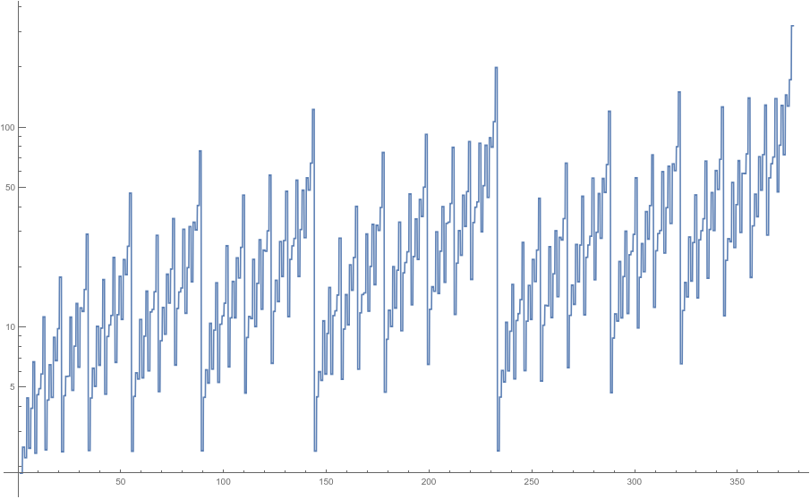
They observed that the peaks of seem to be at with a local minimum at for every . Additionally, they observed that appears to be minimal when , an observation that extends to with . This led them to the following two conjectures.
-
(i)
Let where denotes the –th Fibonacci number. Then we have
(9) -
(ii)
Let , . Then we have
(10)
We will prove these conjectures here, also extending (9) to with .
Theorem 2.
Let , . The following statements hold.
-
(i)
Let be a natural number such that , . Then we have
(11) -
(ii)
We have
(12)
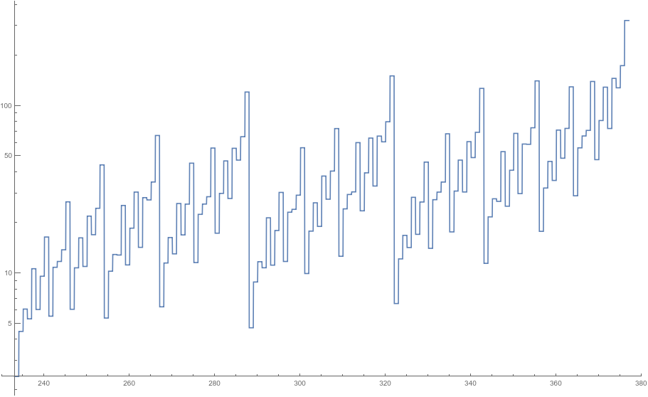
on a logarithmic scale.
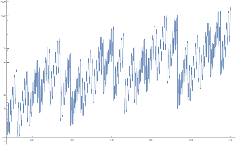
on a logarithmic scale.
Both statements (i) and (ii) of Theorem 2 are optimal for quadratic irrationals with period length in the sense that they cannot be extended to with : By Theorem A, we know that in that case , already making (12) impossible to hold. Since Aistleitner, Technau and Zafeiropoulus showed in [3] that for any we have , also must be violated for any and some sufficiently large. By a similar argument, we see that eventually fails as well.
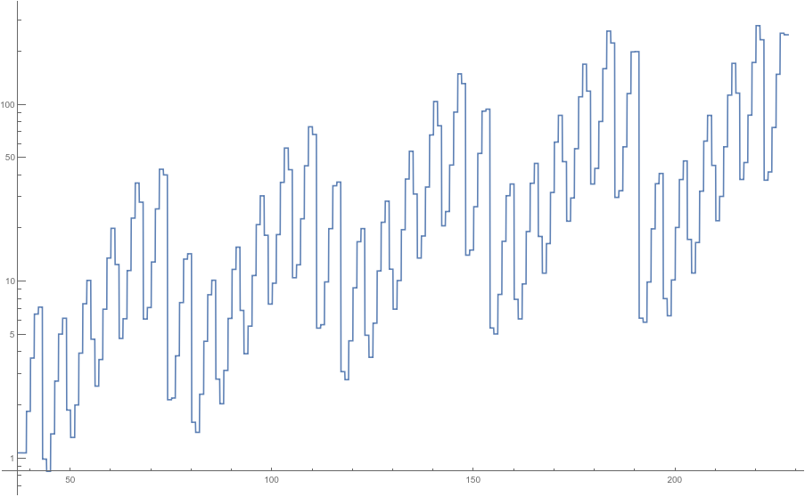
on a logarithmic scale.
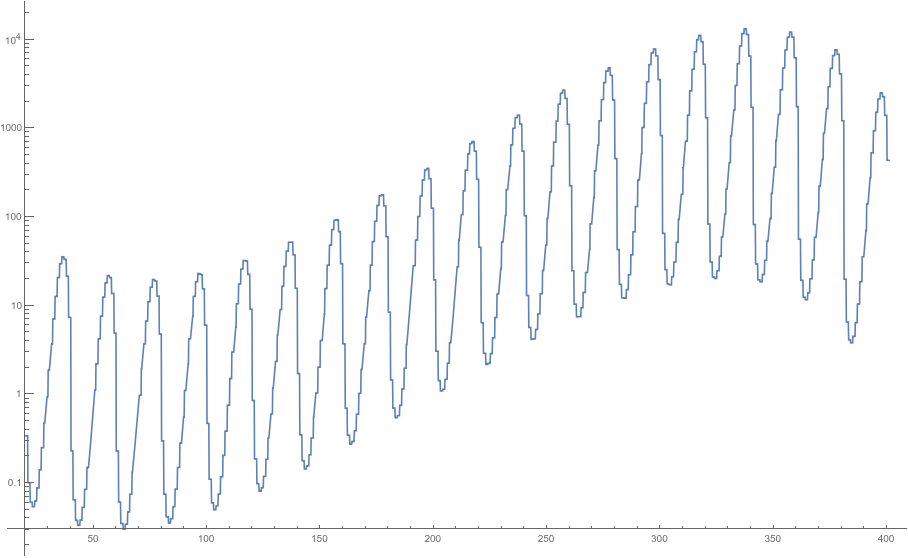
on a logarithmic scale.
1.2. Directions for further research
Recently, Grepstad, Neumüller and Zafeiropoulos [17] studied the behaviour of for quadratic irrationals of the form . They proved that if , then
| (13) |
Actually, they show that the properties in (13) are invariant under the Gauss map
, so the statement can be extended to
arbitrary quadratic irrationals
with .
It remains an open question how far the condition can be relaxed. Numerical experiments suggest that is sufficient to have (13), which would be in accordance with Theorem A (ii) where the period length is .
Grepstad and Neumüller [19] showed that for purely periodic quadratic irrationals with period length , and , exists,
hence we can argue similarly to before that whenever (13) is fulfilled, the statements
from Theorem 2 cannot hold. However, the converse does not need to be true since Theorem 2 considers the behaviour of in finite ranges. So one can ask which quadratic irrationals fulfill and , but do not fulfill (11) and (12).
It is clear that this holds for irrationals with large partial quotients in the pre-period, so a characterization of quadratic irrationals fulfilling (11) and (12) will probably
only consider irrationals with purely periodic continued fraction or will need to consider the value of
.
1.3. Notation
Given two functions we write , and when
respectively. Given a real number we write for the fractional part of and for the distance of from its nearest integer. For being a logical expression, we write
2. Preliminaries
2.1. Continued fractions
We will quickly recall all facts needed in this paper about continued fractions, stating several identities used in the subsequent proofs. For a more detailed background, see e.g. [4, 28, 29]. Every irrational has a unique infinite continued fraction expansion with convergents fulfilling the recursions
| (14) |
with initial values . From (14), one can deduce that holds for any , so in particular,
| (15) |
Furthermore, are coprime and thus,
| (16) | ||||
| (17) |
is bijective. Additionally, we have
| (18) |
We know that approximates very well. Indeed, we have the following well-known inequalities for :
| (19) |
| (20) |
| (21) |
Fixing an irrational , the Ostrowski expansion of a non-negative integer is the unique representation
| (22) |
with the additional rule that whenever .
We proceed to the special case of irrationals of the form . Here we have the following well-known identities:
| (23) | ||||
| (24) | ||||
| (25) | ||||
| (26) |
2.2. Shifted Sudler products
We follow a decomposition approach that was implicitly used already in [18] to prove and more explicitly, in later literature [1, 2, 3]. Here, the Sudler product is decomposed into a finite product with factors of the form
| (27) |
where . We will first study the case where , which is the easiest case, and will discuss the general case afterwards. Due to the well–known fact that , we will work with shifted Sudler products of the form
Let be a positive integer and let be the unique integer such that . The Ostrowski expansion (also called Zeckendorff expansion for the case of the Golden Ratio) simplifies to
for some appropriate where
Denoting
, we can write
| (28) | ||||
| (29) |
where . Using (24), we obtain
| (30) |
By (25) and , we have
so we get by (26) the upper bound
| (31) |
and the lower bound
| (32) |
We see that we have reduced the problem of finding a reasonable lower bound on to the problem of finding lower bounds on for and in a given interval.
Generalizing this idea to the case of quadratic irrationals with continued fraction period length , we let
be the Ostrowski expansion of a positive integer . Following the argument in the proof of [3, Lemma 3], we define
to obtain
| (33) | ||||
| (34) |
where
| (38) |
and
| (39) |
So again we have reduced finding bounds on to the problem of finding bounds for where lies in a specified interval. The tools to obtain these bounds will be developed in the next section.
2.3. Limit function
As mentioned in the introduction, Mestel and Verschueren [26] showed that converges to some positive constant , a result generalized by Aistleitner, Technau and Zafeiropoulus by the following theorem:
Theorem B (Aistleitner, Technau and Zafeiropoulus [3, Theorem 4]). Let be a positive integer and let . For every , the limit
exists. The convergence is uniform on compact intervals.
The authors also give a rather long, closed expression for which helped them to approximately compute and in particular, to calculate .
In a recent paper, Aistleitner and Borda [2] quantified this convergence. Their result holds for arbitrary quadratic irrationals , but we state the theorem only for irrationals whose continued fraction expansion has period length :
Theorem C (Aistleitner, Borda [2, Theorem 4]). Let and let
| (40) |
where
Furthermore, let be a compact interval. Then
| (41) |
with implied constants only depending on and .
With a more detailed analysis, we will show that the multiplicative error in (41) can be decreased further for arbitrary quadratic irrationals.
Lemma 3.
Let be as in Theorem C. Then we have
| (42) |
with implied constants only depending on and which are explicitly computable.
We note that our method of proof is not restricted to quadratic irrationals of the form ; taking other quadratic irrationals leads to other implied constants, but the order of convergence remains the same. For this reason, we can improve the convergence rate from (41) to for arbitrary quadratic irrationals.
As a corollary of Theorem C respectively Lemma 4, we can find for any given and any interval an explicitly computable such that for all and any
| (43) |
This implies that
| (44) |
fulfills the property for all . However, we can still not take as our computable lower bound due to the following two reasons:
-
•
We do not know the exact value of the perturbation , but only an interval where lies in.
-
•
is defined as an infinite product and is therefore not exactly computable.
To solve the first issue, we can show that and are both pseudo-concave on zero-free intervals. As a reminder, we call a function to be pseudo-concave on an interval if it fulfills
| (45) |
It is an easy exercise to check that -concavity implies pseudo-concavity, a fact that was used in [3] to show that is pseudo-concave on zero-free intervals. Similarly, we see by elementary calculus that for any
| (46) |
as long as is no zero of . Hence, also is pseudo-concave on zero-free intervals. Pseudo-concavity is stable under scaling, adding constants and taking a minimum, so we can conclude that (45) also holds for . Therefore, we can estimate
| (47) |
Concerning the second issue, we see that it suffices to compute a finite truncation of the infinite product to obtain a sufficiently small approximation error as shown by the following lemma.
Lemma 4.
Let be defined as in (40), , a compact interval. Writing
we have for sufficiently large that
where the implied constant only depends on and and is explicitly computable.
So we find for any and any zero-free interval an explicitly computable positive integer such that for any
| (48) |
Defining
| (49) |
where , we get from the discussion on pseudo-concavity that
for any , with being computable in finitely many steps. In some cases, this estimate will turn out to be too coarse, since takes much smaller values than for . Hence, we define analogously to (49) the function
| (50) |
Using the same arguments as for , we obtain
for any . We will apply these considerations to where . Note that still implicitly depend on several parameters; choosing very small leads to rather large values for and thus, to larger computational effort to calculate . In the following corollary, we balance this choice in a way such that and are small enough to obtain good enough lower bounds to prove Theorem 1 and 2, but are large enough such that and remain small enough to compute with reasonable computational effort. To avoid repeating the arguments five times, we will only consider the easiest case, that is the case of the Golden Ratio with , for seeing the main structure, as well as the most delicate case, that is, . The intermediate cases where can be treated analogously.
Corollary 5.
Let be defined as in Lemma 4. Then we have the following.
-
(i)
Let , . Then
(51) -
(ii)
Let , . Then
(52)
Note that the intervals are chosen in a way such that every perturbation possibly appearing in the decompositions in Section 2.2 lies in the corresponding interval, which follows from (31) and (32) for the Golden Ratio respectively (38) and (39) in the case . To avoid breaking the flow of the paper, we postpone the rather long proofs of Lemma 3, Lemma 4 and Corollary 5 to Section 5.
3. Proofs for the case of the Golden Ratio
We will prove Theorem 1 and Theorem 2 together. In fact, we prove the following three statements for .
For , we have
| (53) |
For and , we have
| (54) |
For and , we have
| (55) |
Theorem 1 follows immediately from (4), (54) and (55) whereas the statement (11) of Theorem 2 follows from (54) and (55) and (12) follows from (53) and (54). Note that in (55), we actually prove something stronger than needed in the theorems: for Theorem 1, we only need (55) to hold for sufficiently large , and for Theorem 2 it would suffice to have .
Readers who are familiar with the reflection principle, which is the reason behind the connection between the behaviour of and ) (see [15, proof of Lemma 1] or more explicit in [3]) might assume that one can extend (55) to
| (56) |
This can indeed be proven for the case of the Golden Ratio, but interestingly fails to hold for , even when assuming sufficiently large. One can show for example that for and and , we have . This can be proven with the tools provided in this paper, but will not be elaborated further.
Returning to the proofs of (53) – (55), we will concentrate first on the case where , that is the case of the Golden Ratio. Since , we assume for easier notation and . We verify (53) – (55) for all and hence, , by explicit computations, so we will assume throughout the rest of this section that .
We start with proving (53) as a warm-up. Let , then we have where is defined as in (50) with parameters determined by Corollary 5. During the rest of this paper, we will always mean by the functions with these fixed parameters, also suppressing the dependence of on respectively for the sake of readability. Numerical evaluation yields which proves (53).
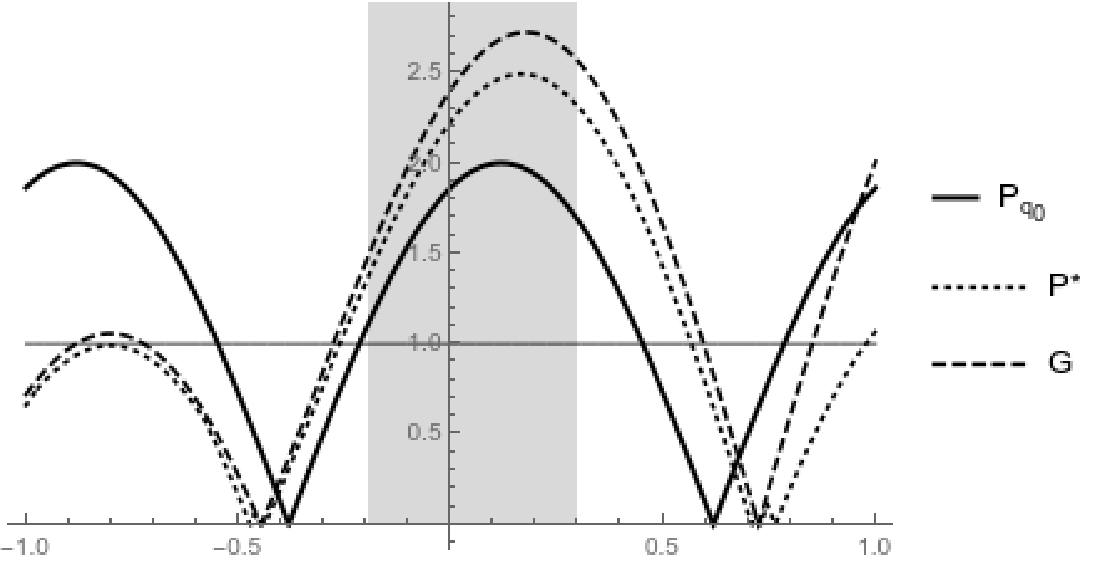
To prove (54), let be the Zeckendorff expansion of . By the discussion in Section 2.2 we can write
| (57) |
where . We obtain by actual computation that
so we can deduce that , and thus, follows immediately.
| (58) |
so we see that (55) is equivalent to showing that
| (59) |
Since (55) holds trivially for , we can write
in its Zeckendorff expansion with . Using the arguments from Section 2.2, with substituted by and the additional perturbation coming from , we see that
| (60) |
where
| (61) |
with . The only difference to (30) is the opposite sign in the last summand above. However, it can be shown that we still have for : by (26), we have
so the additional perturbation equals precisely the worst case possible for the estimate on higher orders of appearing in (31) and (32). Therefore, we can deduce immediately that holds for any . These arguments are the key for the connection between and established in [3]. There, it sufficed to prove that the left-hand side of (59) is bounded away from , which is not enough to prove (55): in fact, for , we have
| (62) |
so it suffices to prove
| (63) |
We consider the following case distinction, depending on the Ostrowski coefficients of , showing that we fulfill (63) in any case.
-
•
Case 1: , . In this case, we have
Since for , we can deduce that .
-
•
Case 2: , . Observe that for , the sum in (61) simplifies to the single term . Thus, we obtain the better estimates
(64) which imply
(65) -
•
Case 3: , . We have for any that
(66) Since and all other factors are bounded from below by , we obtain (63).
-
•
Case 4: , . Directly bounding by and by is not enough to obtain a value that exceeds , so we have to argue differently. First note that implies . Since , we have or , so in both cases at least one of the perturbations is very close to , improving the estimates sufficiently:
If , we have
and by , the result follows.
4. Proofs for quadratic irrationals of the form
Here we prove (53) – (55) for the case where . The general layout of the proof remains similar to the one for the Golden Ratio, however, we have to be more careful in the numerical analysis. As before, we check numerically with computer assistance that (53) – (55) hold for and allowing us to assume from now on that .
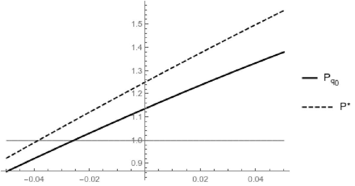
Proving (53) is still straightforward: We have , so (53) follows by the same argument as in the case of the Golden Ratio (see Figure 5).
Next, we proceed to show (54). We recall from (34) that if is the Ostrowski expansion of , we can write
| (67) |
with
| (68) |
where . The analysis here is more tedious than in the Golden Ratio case since the limit function does not fulfill for all appearing perturbations , so in particular, we cannot argue that .
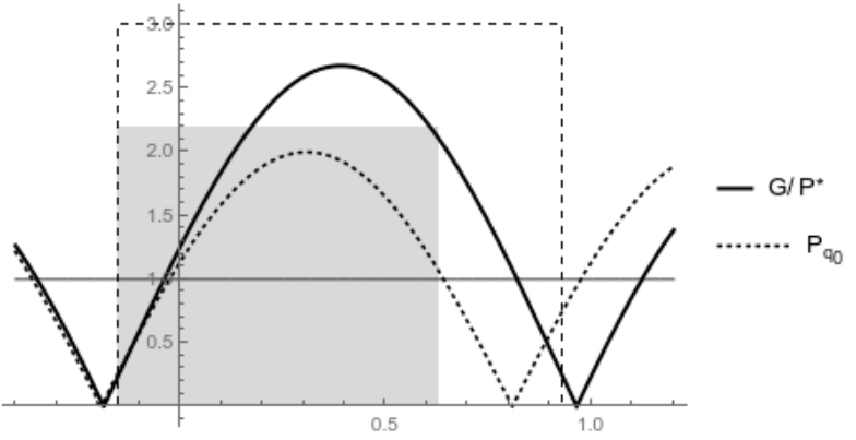
However, as we see in Figure 6, we only have if is either very small or very large. Looking at (68), we see that is very small if and is “large”, that is or . We will see that are values located in an area where is close to its peak, exceeding by a large margin. As the factors are factors of the product when or , these factors will overcompensate the factor which might be smaller than , which results in exceeding in most cases. Similarly, if the perturbation is very large, this implies that and , again yielding overcompensating factors that allow us to deduce that the above product exceeds in most cases. For a detailed explanation and an explicit example of this phenomenon, we refer to [3, p.28 – 30]. Following this observation, we write
| (69) | ||||
| (70) |
with the convention . For shorter notation, we define
| (71) |
It follows immediately that showing is equivalent to proving
| (72) |
To prove that, we will show that most factors fulfill . If this cannot be shown for some fixed , we will prove that there is another factor for which is much larger than such that . This approach is very similar to the proof of [3, Lemma 3]. However, in [3] it suffices to show that (or ) holds whenever is sufficiently large and for all where is another, arbitrary large constant. As we cannot make these assumptions here, we will work with the functions and and not with arbitrary close approximations to the limit function . Since , we need to distinguish even more cases than already considered in the delicate analysis in [3]. Note that estimates on need a special treatment when is small: We might not be able to use as lower bound, but need to consider the weaker bound . Additionally, the error appearing in the estimate for (see (68)) gets larger the smaller is. Therefore, we need to distinguish several cases depending on whether or not.
Estimates for
In view of (68) and (71), we have perturbations of the form for with
| (73) |
where
| (74) |
Since , we can deduce that
| (75) |
If , we will use the estimate for upper bounds and for lower bounds. If , we use the converse inequalities for upper respectively lower bounds. Note that these values are very small, so they will not play a main role. Using (26), we obtain
| (76) |
Since , we have in particular , and thus, we know by the properties of the Ostrowski expansion that . This leads to
| (77) |
Since is a lower bound on the pseudo-convex function , we can deduce from (75), (76) and (77) that if ,
| (78) |
Concerning , we see by similar arguments that
| (79) |
with being or , depending on the value of . Looking at (71), we observe that the value of heavily depends on the coefficients , so we will make a case distinction depending on the values of those coefficients. The values on the right-hand sides of (78) and (79) are used as lower bounds in most cases stated below, so we collect these lower bounds for and in the following table.
| k | If , then | If , then |
|---|---|---|
| 0 | - | 1.20 |
| 1 | 1.47 | 0.97 |
| 2 | 2.37 | 0.73 |
| 3 | 2.25 | 0.48 |
| 4 | 1.12 | 0.24 |
Case 1: . In this case, . From Table 1 we obtain .
Case 2: . As in Case 1, we have , but the lower bound for from (79) is not enough to show . Fixing the values of , we obtain the sharper estimate
| (80) |
with equality to the bound from (79) in case of . We will consider two subcases, depending on :
-
–
Case 2a: or : In this case, (80) is good enough to deduce .
- –
Case 3: . In this case we have , so by Table 1 we have
Case 4: . This gives , which leads to .
Case 5: . We obtain and so we can deduce .
Case 6: . Note that this case covers completely since implies .
-
–
Case 6a: : Then the product for is empty and hence, .
-
–
Case 6b: . , so we obtain .
-
–
Case 6c: . and thus, .
-
–
Case 6d: . gives
. -
–
Case 6e: . which leads to
To conclude, we see that the only case where we cannot show that is Case 2b, which forces the factor to be in one of the Cases 6b – 6e. We see that this implies , so we deduce therefore, follows.
Estimates for
For , we have
If , we can apply Case from above and are done. If, however, , we cannot apply the estimate , but will compute directly. We can take the estimates for from (79) with the adjustment that can now only be bounded from above by . The correspondingly changed values in the table look as follows:
| k | If , then |
|---|---|
| 0 | 1.10 |
| 1 | 0.89 |
| 2 | 0.68 |
| 3 | 0.46 |
| 4 | 0.23 |
Going through the calculations in Cases with these slightly changed values from Table 2 shows that this is still sufficient to prove . Concerning Case 2, which was already the most intricate one before, we have to argue differently. We see that without making additional assumptions, we can only prove that . As above, we will find a factor which overcompensates the factor and differs from the factors used to overcompensate Case 2b for any . However, we cannot fix the as in the case with , but will depend on possibly all Ostrowski coefficients. We consider the following cases:
-
–
Case : There exists some such that . Taking the smallest with that property, we know that . This leads for to Case 1 where we have proven that . Thus, .
-
–
Case : for all and there exists some such that . This implies that for we are either in Case 4 or Case 5 where we have shown that , so again we can prove
-
–
Case : for all . This implies in particular , so we can improve the estimate (79) to
(81) This leads to the sharper estimate . By the assumption , we see that is in Case 2 or Case 3. If is in Case 3, we obtain from the discussion above that which suffices to show If we are in Case 2, we use the improved bound (81) (with instead of ) to get , again deducing .
As mentioned, the factor appearing in Cases is not used by some to overcompensate Case 2b: Overcompensating factors for Case 2b always come from Case 6, whereas is always in one of the Cases 1 – 5.
Estimates for
Observe that by definition, , so here we are always in Case 6a – 6d. Case 6a is an empty product, which is defined to be equal to , so we can concentrate on the case where . Using estimates as in (78) and (79), we obtain
which implies that . Therefore, we have .
Summing up all estimates on for , we obtain (72), and thus, follows.
Proof of (55).
We proceed to prove that for all we have
| (82) |
To do so, we apply the same procedure as done in (59) for the Golden Ratio to see that (55) is equivalent to
| (83) |
Let be the Ostrowski expansion of , possibly with leading zero coefficients. By an analogous argument as in (69), we obtain
| (84) |
where
| (85) |
Accordingly, we get
| (86) |
which shows us that we can interpret as the “normal” defined in (36) with an additional negative Ostrowski coefficient . This additional perturbation will only contribute significantly when is very small. This leads to the following lemma:
Lemma 6.
Let
with as before and assume that or . Then we have
| (87) |
Proof.
If , we see analogously to the Golden Ratio case that the additional perturbation vanishes in the estimate for the geometric series: by (26), we have so the additional perturbation equals precisely the worst-case higher-order estimates used in (76) and (77). Therefore, we can use Table 1 for to deduce by the same arguments as in (54) that we have or, if Case 2b applies, . Note that if , we cannot consider to show (87), hence we simply take the estimate if Case 2b applies. We observe that by the assumptions made in Case 2b, at most one of can be in this case. This factor is bounded from below by , with the other factor exceeding . Since the special cases can be treated completely analogously to the proof of (54), we conclude the proof of the lemma.
Returning to the proof of (55), we argue similarly to the case of the Golden Ratio: we need to obtain factors being significantly larger than to gain the extra factor for in (83). Bounding by
turns out to be too coarse, so we will use a better bound, depending on the Ostrowski coefficients of .
Proposition 7.
Let and be the Ostrowski expansion of , possibly with leading zero coefficients. Then
| (88) |
Proof.
By the properties of the Ostrowski expansion, we obtain
which implies by the recursion formula from (14) that
Applying (14) again, we get , and the result follows.
Leaving the possibility of for the moment aside, we will show that the additional factor exceeding comes from : we recall from Cases 3 – 6 above that a large leads to a large factor , significantly exceeding , a fact which will hold for as well. So if is large, we know that or has to be large, and thus, exceeds significantly. If is small, then it suffices that stays just above . To be more specific, we show the following lemma:
Lemma 8.
Let as above and assume we have or . Then
| (89) |
Proof.
Setting , we obtain from (36) that for ,
which leads to
| (90) |
Note that
where
| (91) | ||||
| (92) |
with reverted inequality symbols for (92) in case of . Since , we can deduce that and if . Computing lower bounds for as in Cases 1 – 6 above leads to the following table:
| k | If , | If , | If | |||
| 0 | - | 1.20 | 1.20 | - | 1.125 | 1.35 |
| 1 | 2.37 | 0.97 | 1.425 | 1.47 | 1.422 | 1.8 |
| 2 | 2.66 | 0.73 | 2.54 | 3.48 | 1.93 | 2.7 |
| 3 | 2.25 | 0.48 | 4.44 | 9.26 | 3 | 5.4 |
| 4 | - | 0.24 | - | 20.85 | 6.75 | - |
We see that holds whenever , but might fail for . In these cases, we will see that gives us another factor that exceeds significantly, closing the gap between and : note that implies , so we obtain that
where
| (93) | ||||
| (94) |
The special case
We are left to consider the special case which implies . We set and assume first that . This implies that is in Case 1 and thus, . Since , we see that
a range where we can prove that . Similarly to Lemma 6, we show that
with the following adjustments:
For , we cannot use the case distinction in Cases , so we can only deduce .
Recall that in Lemma 6 (which treated the case or ), we found no overcompensating factor if . This translates now to finding no compensating factor if . However, by construction, rules out an appearance of Case 2b there, so we do not have to consider an additional factor below . Since
is an empty product and , we can complete the case and are left with the possibility that . We see that with
Using instead of , we can compute that . Since the only other non-trivial factor from (84) is , we have finished the last case and therefore, also the proof of (55).
5. Proofs of Lemma 3, Lemma 4 and Corollary 5
Proof of Lemma 3
We will follow the main structure of the proof in [2, Theorem 4], improving at some points the estimates by refined arguments and making the constants hidden in the explicit. Note that we do not aim to determine the best constants possible, but are contented with sufficiently small constants to deduce Corollary 5 for small enough to compute and with acceptable computational help. The following proposition will be used several times in the proof of Lemma 3 to find reasonable bounds on products whose factors are close to 1.
Lemma 9.
-
(i)
Let and . Then
(95) -
(ii)
If and , then
(96) -
(iii)
If , then
(97)
Proof overview
We will prove the inequality
with explicitly specified constants. This is the inequality we need to prove the main results of this paper. The other inequality can be shown by very similar methods (with different explicit values of the implied constants). For better readability, we define and . Note that is –periodic and an even function, facts that will be used implicitly several times below. Taking the last factor of out of the product and using (18), we obtain
| (99) |
Observe that the factors on the right-hand side of (99) only depend on the residue class of . Using properties (15) and (16), we deduce
We see that
so we can write
| (100) |
Combining the –th and () –th factor of (100) for and using the trigonometric identity , we obtain
| (101) |
with an additional factor
| (102) |
if is even.
Next, we consider a monotonically non-decreasing integer-valued function fulfilling , but , which will be optimized later. Furthermore, let be a sufficiently large integer, depending only on and . We denote
and
We split the factors on the right-hand side of (101) into several groups and prove Lemma 3 via the following steps:
-
Step 1:
(103) -
Step 2:
(104) -
Step 3:
(105) -
Step 4:
(106) -
Step 5:
(107) -
Step 6:
(108)
Combining Steps 1 – 6, we deduce
| (109) |
Proof of Step 1
For better readability, we define
If is sufficiently large, then and thus we can estimate
Proof of Step 2
If is large enough such that , we can remove for the absolute values of . We use the trigonometric identity
| (110) |
to get
| (111) |
Since quadratic irrationals have bounded partial quotients, we see from (19) that there exists some fixed such that . Therefore, we have
which leads with to
| (112) |
By for we get that
| (113) |
Combining these estimates, we obtain
where
For large enough, we have , so
| (114) |
By Proposition 9 (iii), we get
| (115) |
To bound the first product in (114), we apply partial summation and employ the monotonicity of on to obtain
| (116) |
where and . A short elementary computation shows that we can bound the variation by
Using a standard discrepancy estimate in the form of [14, Theorem 1.1], we have for
where denotes the star-discrepancy. Applying Koksma’s inequality yields
| (117) |
For an introduction on discrepancy and Koksma’s inequality, we refer the reader to [23]. Using and Proposition 9 (i), we obtain
| (118) |
| (119) |
Proof of Step 3
Observe that for sufficiently large and , one can remove the absolute values of
and therefore,
where
| (120) |
Due to a result in Ostrowski’s famous work [27], we get for the estimate
If , we use the triangle inequality and to obtain
Applying summation by parts and , we get
| (121) |
For sufficiently large, the left-hand side of (121) is bounded by , and thus, Proposition 9 (ii) gives
| (122) |
For and we use the estimate . Following the same steps as in the case, we end up with an error term as in (122), but with substituted by . Note that this argument also works for arbitrary quadratic irrationals since Ostrowski’s estimates can be generalized to all irrationals with bounded partial quotients.
Proof of Step 4
Before we start with the actual proof of Step 4, we need a technical, but nevertheless important lemma to find good bounds for terms of the form under certain conditions on . This lemma gives us a power saving in comparison to applying the estimate for all terms independently as done in [2, Theorem 4], leading to the improvement of the convergence rate in Lemma 3.
Lemma 10.
Let and
| (123) |
| (124) |
Then we have
| (125) |
Proof.
By Taylor approximates and , we have
Since implies that , we obtain
| (127) |
Concerning , we use Taylor approximations and to obtain
which leads by to
| (128) |
Note that (124) implies
Returning to the proof of Step 4, we set
Note that where are defined as in the proofs of Step 1 and 2. This implies that for with chosen sufficiently large, we can apply Lemma 10 to obtain
| (131) |
Since , we have for sufficiently large that
This implies that the error in the last product of (5) can be bounded by
| (132) |
with . If is large enough, then the right-hand side of (132) can be bounded from above by , so we get by Proposition 9 (iii) that
| (133) |
We are left to compare
with the product
Writing
we see that
| (134) |
From the identities (24) and (25), we can deduce that for sufficiently large
| (135) |
To treat , we will show that for sufficiently large ,
| (136) |
that is, the function has no discontinuity between and . Such a “jump” would imply that there exists an integer such that
| (137) |
We assume the former to be the case, with the other one working analogously. Let with . By (19) and (20), we obtain
So we have by (137)
| (139) |
Next, we define
We argue similarly to (135) to show that
| (140) |
Finally, combining (139) and (140) and assuming that is large enough such that , we can deduce that
| (141) |
For sufficiently large, the error term in (141) is bounded from below by , so we can apply Proposition 9 (iii) together with (133) to obtain
| (142) | ||||
Proof of Step 5
We will imitate a part of the argument from Step 4. However, here we cannot guarantee that the assumptions of Lemma 10 are fulfilled. So we use the weaker estimate
| (143) |
on to obtain
| (144) |
where the implied constant depends on . By the same arguments as in Step 4, we can prove the inequalities (139) and (140). Since we cannot assume that , we now get from
| (145) |
an additive error of order .
Proof of Step 6
follows. This finishes the proof of Lemma 3.
Proof of Lemma 4
The proof of Lemma 4 works in a similar fashion to Step 3 of Lemma 3, although this time we need a lower bound on . If is sufficiently large, we can remove the absolute values in the definition of and obtain
| (148) | ||||
| (149) |
| (150) |
We see that for sufficiently large, (150) can be bounded by , hence applying Proposition 9 (ii) leads to
| (151) |
Again, for , we can replace in the estimate by .
Proof of Corollary 5
We can explicitly compute the constants used in the proof of Lemma 3 for the Golden Ratio respectively the quadratic irrational , and specify all the errors from Steps 1 – 6. It turns out that and for the Golden Ratio respectively for are large enough to fulfill all assumptions on to be “sufficiently large” that are made in the proofs of Lemmas 3 and 4. We see that the errors from Steps are in , and since all constants are small and since we can choose in both cases , we can bound both the additive and the multiplicative error by in the Golden Ratio case and by in the case . To not repeat all arguments from above again, we will only address Steps and consider the main error terms there. In the case of the Golden Ratio, we can bound , and thus we get for Step 2 an error bounded by Step 3 leads to an error bounded by , Step 4 to . Adding these errors, we obtain the result for the Golden Ratio. Similarly, we can treat the case : Here we can bound which leads for Step 2 to an error bounded by For Step 3, we can bound the error by , for Step 4 by . Again, the result follows immediately from adding these errors.
6. Acknowledgements
The author would like to thank Christoph Aistleitner for helpful discussions and for suggesting this direction of research.
References
- [1] C. Aistleitner, B. Borda, Maximizing Sudler products via Ostrowski expansions and cotangent sums, pre-print: arXiv:2104.01379.
- [2] C. Aistleitner, B. Borda, Quantum invariants of hyperbolic knots and extreme values of trigonometric products. pre-print: arXiv:2006.08578v2.
- [3] C. Aistleitner, N. Technau and A. Zafeiropoulos On the order of magnitude of Sudler products, pre-print: arXiv:2002.06602.
- [4] J. Allouche, J. Shallit, Automatic Sequences: Theory, Applications, Generalizations. Cambridge University Press, 2003.
- [5] F.V. Atkinson, On a problem of Erdös and Szekeres. Canad. Math. Bull., 4 (1961), 7–12.
- [6] A. Avila, S. Jitomirskaya, The Ten Martini Problem. Ann. of Math. (2) 170 (2009), no. 1, 303–342.
- [7] A. Avila, S. Jitomirskaya, C.A. Marx, Spectral theory of extended Harper’s model and a question by Erdös and Szekeres. Invent. Math. 210 (2017), no. 1, 283–339.
- [8] J.P. Bell, P.B. Borwein, L.B. Richmond, Growth of the product . Acta Arith. 86 (1998), no. 2, 155–170.
- [9] J. Bell, Estimates for the norms of sines and cosines. J. Math. Anal. Appl., 405 (2013), no. 2, 530–545.
- [10] J. Bourgain, M.C. Chang, On a paper of Erdöss and Szekeres. J. d’Anal. Math., 136 (2018), no. 1, 253–271.
- [11] S. Bettin, S. Drappeau, Limit laws for rational continued fractions and value distribution of quantum modular forms. pre-print: arXiv:1903.00457.
- [12] S. Bettin, S. Drappeau, Modularity and value distribution of quantum invariants of hyperbolic knots. Math. Ann. (2021).
- [13] S. Bettin, S. Drappeau, Partial sums of the cotangent function. J. Théor. Nombres Bordeaux 32 (2020), 217-230
- [14] K. Doi, N. Shimaru, K. Takashima, An upper estimate for the discrepancy of irrational rotations. Acta Math. Hungar. 152, 109–113 (2017).
- [15] P. Erdös, G. Szekeres, On the product . Acad. Serbe Sci. Publ. Inst. Math. 12 (1958), 29–34.
- [16] Q G. Freiman, H. Halberstam, On a product of sines. Acta Arith., 49 (1988), no. 4, 377–385.
- [17] S. Grepstad, M. Neumüller, A. Zafeiropoulos, On the order of magnitude of Sudler products II. pre-print: arXiv: 2109.04342
- [18] S. Grepstad, L. Kaltenböck, M. Neumüller, A positive lower bound for . Proc. Amer. Math. Soc. 147 (2019), 4863–4876.
- [19] S. Grepstad, M. Neumüller, Asymptotic behaviour of the Sudler product of sines for quadratic irrationals. J. Math. Anal. Appl. 465 (2017), no. 2, 928–960.
- [20] S. Grepstad, M. Neumüller, On the asymptotic behaviour of the sine product . pre-print: arXiv:1909.00980.
- [21] M.N. Kolountzakis, A construction related to the cosine problem. Proc. Amer. Math. Soc. 122 (1994), no. 4, 1115–1119.
- [22] M.N. Kolountzakis, The density of Bh[g] sets and the minimum of dense cosine sums. J. Number Theory 56 (1996), no. 1, 4–11.
- [23] L. Kuipers, H. Niederreiter, Uniform Distribution of Sequences, Wiley (1974).
- [24] D. Lubinsky, {The size of for on the unit circle}, J. Number Theory 76 (2) (1999), 217–247.
- [25] D. Lubinsky, E.B. Saff, Convergence of Padé Approximants of Partial Theta Functions and the Rogers- Szegö Polynomials. Constr. Approx. 3 (1987), no. 4, 331–361.
- [26] B. Mestel, P. Verschueren, Growth of the Sudler product of sines at the golden rotation number. Journal of Mathematical Analysis and Applications, 433(1) pp. 200–226.
- [27] A. Ostrowski Bemerkungen zur Theorie der Diophantischen Approximationen. Abh. Math. Semin. Univ. Hamburg. 1, 77–98 (1922).
- [28] A.M. Rockett, P. Szüsz Continued fractions. World Scientific Publishing, River Edge, NJ, 1992.
- [29] W.M. Schmidt Diophantine approximation. Lecture Notes in Mathematics, 785. Springer, Berlin, 1980.
- [30] C. Sudler Jr. An estimate for a restricted partition function. Quart. J. Math. Oxford Ser. 15 (1964), 1–10.
- [31] E.M. Wright Proof of a conjecture of Sudler’s Quart. J. Math. Oxford Ser. 15 (2) (1964), 11–15.
- [32] D. Zagier, Quantum modular forms. Quanta of maths, 659–675, Clay Math. Proc., 11, Amer. Math. Soc., Providence, RI, 2010.