Joint Stereo 3D Object Detection and Implicit Surface Reconstruction

Abstract

We present a new learning-based framework S-3D-RCNN that can recover accurate object orientation in SO(3) and simultaneously predict implicit shapes for outdoor rigid objects from stereo RGB images. In contrast to previous studies that map local appearance to observation angles, we explore a progressive approach by extracting meaningful Intermediate Geometrical Representations (IGRs) to estimate egocentric object orientation. This approach features a deep model that transforms perceived intensities to object part coordinates, which are mapped to a 3D representation encoding object orientation in the camera coordinate system. To enable implicit shape estimation, the IGRs are further extended to model visible object surface with a point-based representation and explicitly addresses the unseen surface hallucination problem. Extensive experiments validate the effectiveness of the proposed IGRs and S-3D-RCNN achieves superior 3D scene understanding performance using existing and proposed new metrics on the KITTI benchmark. Code and pre-trained models will be available at this https URL.

Figure 1: Given a pair of stereo RGB images, S-3D-RCNN can detect rigid 3D objects and predict their implicit shapes with one forward pass. (a) Alpha-blended image pair to show the disparities. (b) 3D object proposals shown as 3D bounding boxes. (c) Shape predictions for the detected objects. (d) Estimated surface normal of the nearby object. (e) The predicted implicit shape supports a spatially-varying resolution.

I Introduction

“The usefulness of a representation depends upon how well suited it is to the purpose for which it is used”. –David Marr [1]

Estimating 3D attributes of outdoor objects is an important task for image-based autonomous perception and augmented reality. Despite the binocular human visual system can recover multiple 3D object properties effortlessly from a glance, this task is challenging for computers to accomplish. The difficulty results from a lack of geometry information after image formation, which causes the semantic gap between RGB pixels and unknown geometrical quantities. This problem is even exacerbated by the complexities of different unknown attributes and a huge variation of object appearances. To address this problem, Marr pointed out the importance of representations and further proposed the representational framework of vision. In the framework, intermediate representations called the 2.5D sketch are built upon low-level pixels and are later lifted to 3D model representations. Recently, advances in deep learning greatly facilitated the representation learning process from data, where a neural network can fit an arbitrarily complex function. However, how to design effective intermediate representations toward accurate and robust outdoor 3D attribute recovery is still task-dependent and under-explored.

The conference version of this study [2] addressed the aforementioned problem for a single task, i.e., estimating orientation in SO(3) from a single RGB image for a class of rigid objects (vehicle). Instead of directly regressing object orientation from pixels with a black-box neural network, a progressive mapping from pixels to 3D poses was designed inspired by the representational framework of vision. The proposed model, Ego-Net, computed part-based screen coordinates from object part heatmaps and further lifted them to 3D object part coordinates for orientation inference. These intermediate geometrical representations (IGRs) bridge the semantic gap and were shown to be effective for accurate and robust orientation estimation from single-view image inputs.

While the previous study [2] is effective for vehicle orientation estimation, it is limited in several aspects which demands further exploration. Firstly, the approach was demonstrated only for a single-view setting. The difficulty of monocular depth estimation makes it less useful in perception systems and thus an extension to multi-view sensor configuration is highly favorable. Secondly, the approach was only validated for vehicles and not shown for other common articulated objects such as pedestrians. These objects are smaller and have fewer training labels, it would be intriguing whether the proposed IGRs show consistent effectiveness or not. Lastly, the approach can only recover the orientation in a 3D object detection (3DOD) system to predict 3D bounding boxes. A complete and detailed shape description within 3D bounding boxes is desirable for various machine vision applications. For example, an autonomous perception system can give a more accurate collision prediction for an object intruding another object’s 3D bounding box. An outdoor augmented reality system can enable photo-realistic lighting and simulate physics-based surface effects as illustrated by the green ray reflecting on the object surface in Fig. 1(d). These functions cannot be achieved by using 3D bounding boxes to represent objects due to the lack of fine-grained surface normal estimation indicated by the red reflecting ray.

To address these gaps, this study presents an extended model S-3D-RCNN for joint object detection, orientation estimation, and implicit shape estimation from a pair of RGB images. Firstly, we demonstrate the effectiveness of the proposed IGRs in a stereo perception setting, where part-based screen coordinates aggregated from two views further improves orientation estimation accuracy. Secondly, we validate the robustness of the proposed IGRs for other outdoor objects such as pedestrians and cyclists. These tiny objects are underrepresented in the training dataset yet the proposed approach still achieves accurate orientation estimation. Lastly, we propose several new representations in the framework to further extend EgoNet for implicit shape estimation. We formulate the problem of implicit shape estimation as an unseen surface hallucination problem and propose to solve it with visible object point coordinates in the object coordinate system. For quantitative evaluation, we further propose two new metrics to extend the 3DOD evaluation to consider the retrieval of the object surface. In summary, this study extends the previous conference version in various aspects with the following contributions.

• It explored the proposed IGRs in a stereo perception setting and validates the effectiveness of the proposed approach in recovering orientation in SO(3) for two-view inputs.

• It shows the proposed approach is not limited to rigid objects, and has robust orientation estimation performance for other small objects that may have fewer training labels.

• It extends the representational framework in Ego-Net with several new intermediate representations to achieve implicit shape estimation from stereo region-of-interests. To our best knowledge, Ego-Net++ is the first stereo image-based 3D object detection and implicit shape estimation approach for outdoor rigid objects.

• To quantitatively evaluate the proposed implicit shape estimation task, two new metrics are designed to extend the previous average precision metrics so as to be aware of the object surface estimation quality.

We introduce and compare with relevant studies in the next section and revisit Ego-Net in the next section. We further detail extended studies in designing Ego-Net++ followed by experimental evaluations.

II Related Work

Our approach features outdoor environment, orientation estimation, and implicit shape reconstruction. It draws a connection with prior studies in the following domains yet has unique contributions.

Image-based 3D scene understanding aims at recovering 3D object properties from RGB images which usually consists of multiple sub-tasks [3, 4, 5, 6, 7, 8, 9, 10, 11, 12, 13]. Two popular paradigms were proposed. The generative, a.k.a analysis-by-synthesis approaches [14, 15, 9, 16, 17, 18] build a generative model of image observation and unknown 3D attributes. During inference one searches in 3D state space to find an optimum that best explains the image evidence. However, good initialization and iterative optimization are required to search in a state space that is usually high-dimensional. In contrast, the discriminative approaches [19, 20, 21, 22, 23, 24] directly learn a mapping from image observation to 3D representations. Our overall framework can be categorized into the latter yet is unique. Unlike previous studies that are only applicable for indoor environments with small depth variation [25, 7, 26, 27, 18, 28], only consider the monocular camera setting [9, 21, 29, 30], and require PCA-based templates [31, 32, 33, 23, 34] which are limited to a fixed mesh topology [23] or voxel grid [32, 35, 36, 37], our framework can exploit two-view geometry to accurately locate objects as well as enables flexible implicit shape reconstruction for challenging outdoor environments.

Learning-based 3D object detection learns a function that maps sensor input to objects represented as 3D bounding boxes in the camera coordinate frame [38]. Depending on the type of the used sensors, they can be categorized into RGB-based methods [39, 40, 41, 42, 43, 44, 2, 45, 46, 47, 48, 49, 50] and LiDAR-based approaches [51, 52, 53, 54, 55, 56, 57, 58, 59, 60, 61]. Our approach is RGB-based which does not require expensive range sensors. Compared to previous RGB-based methods that can describe objects only up to a 3D bounding box representation, our approach complements them with shape reconstruction capability by predicting detailed, complete, and resolution-agnostic object surfaces.

Learning-based orientation estimation for 3D object detection seeks a function that maps pixels to instance orientation in the camera coordinate system via learning from data. Early studies [62, 63] utilized hand-crafted features [64] and boosted trees for discrete pose classification (DPC). More recent studies replace the feature extraction stage with deep models. ANN [65] and DAVE [66, 67] classify instance feature maps extracted by CNN into discrete bins. To deal with images containing multiple instances, Fast-RCNN-like architectures were employed in [38, 68, 69, 70, 23] where region-of-interst (ROI) features were used to represent instance appearance and a classification head gives pose prediction. Deep3DBox [71] proposed MultiBin loss for joint pose classification and residual regression. Wasserstein loss was promoted in [72] for DPC. Our Ego-Net [2] is also a learning-based approach but possesses key differences. Our approach promotes learning explicit part-based IGRs while previous works do not. With IGRs, Ego-Net is robust to occlusion and can directly estimate global (egocentric) pose in the camera coordinate system while previous works can only estimate relative (allocentric) pose. Compared to EgoNet, Ego-Net++ in this extended study is no longer limited to monocular input images and rigid objects. In addition, Ego-Net++ can further achieve object surface retrieval from images while Ego-Net cannot.

Instance-level modeling in 3D object detection builds a feature representation for a single object to estimate its 3D attributes [21, 73, 74, 75, 23]. FQ-Net [73] draws a re-projected 3D cuboid on an instance patch to predict its 3D Intersection over Union (IoU) with the ground truth. RAR-Net [75] formulates a reinforcement learning framework for instance location prediction. 3D-RCNN [21] and GSNet [23] learn a mapping from instance features to the PCA-based shape codes. Ours Ego-Net++ is a new instance-level model in that we can predict the implicit shape and can utilize stereo imagery while previous studies cannot.

Neural implicit shape representation was proposed to encode object shape as latent vectors via a neural network [76, 77, 78, 79, 80], which shows an advantage over classical shape representations. However, many prior works focus on using perfect synthetic point cloud as inputs. Instead, we study the inference of such representations under a realistic object detection scenario with stereo sensors.

Figure 2: The proposal model $\mathcal{D}$ of S-3D-RCNN. In this implementation, a volumetric 3D scene representation is built from semantic features and cost-volume-based geometric features similar to [33]. An anchor-based object detector processes the Bird’s Eye View feature maps to generate 3D object proposals. Note that Ego-Net++ $\mathcal{E}$ is agnostic to the design choice of $\mathcal{D}$ and can be used with other 3D object detectors.

Figure 3: Model architecture of Ego-Net. A fully convolutional model $\mathcal{H}$ regresses part heatmaps from a 2D patch of a proposal. The heatmaps are mapped to local coordinates with several strided convolution layers. The local coordinates are transformed to screen coordinates $\phi_{g}(\mathbf{x}_{i})$ and mapped to a point-based 3D representation $\psi(\mathbf{x}_{i})$ of a cuboid, whose orientation directly represents egocentric pose in the camera coordinate system. k=33 when q=2 as in Sec. IV-B.

Figure 4: Diagram of Ego-Net++ $\mathcal{E}$ that performs joint orientation and implicit shape estimation for rigid objects. A local cost volume is constructed to estimate disparities. The visible surface is computed from the predicted disparities and an estimated mask. The partial foreground points are normalized to a canonical coordinate system and passed to an encoder-decoder network $Ha$ that infers the missing surface of the object. The complete shape points are passed to an encoder to extract an implicit shape vector, which can be used by a downstream decoder to perform resolution-agnostic surface extraction. A zoomed-in view of the orientation computation is shown in Fig. 8.

III Overall framework

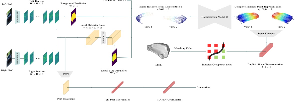
Our framework S-3D-RCNN detects objects and estimates their 3D attributes from a pair of images captured with calibrated stereo cameras. S-3D-RCNN consists of a proposal model $\mathcal{D}$ and an instance-level model $\mathcal{E}$ (Ego-Net++) for instance-level 3D attribute recovery. $\mathcal{E}$ is agnostic to the design choice of $\mathcal{D}$ and can be used as a plug-and-play module. $\mathcal{D}$ is implemented as a voxel-based 3D object detector as shown in Fig. 2. Given an image pair $(\mathcal{L},\mathcal{R})$ captured by stereo cameras with left camera intrinsics $\text{K}_{3\times 3}$, $\mathcal{D}$ predicts $N$ cuboid proposals $\{b_{i}\}_{i=1}^{N}$ as $\mathcal{D}(\mathcal{L},\mathcal{R};\theta_{\mathcal{D}})=\{b_{q}\}_{q=1.}^{N}$ Conditioned on each proposal $b_{i}$, $\mathcal{E}$ constructs instance-level representations and predicts its orientation as $\mathcal{E}(\mathcal{L},\mathcal{R};\theta_{\mathcal{E}}|b_{i})=\bm{\theta}_{i.}$ In addition, for rigid object proposals (i.e., vehicles in this study), $\mathcal{E}$ can predict its implicit shape representation. The following sections first revisit Ego-Net and highlight the newly designed representations in Ego-Net++.

IV Ego-Net: monocular egocentric vehicle pose estimation with IGRs

IV-A Orientation estimation with a progressive mapping

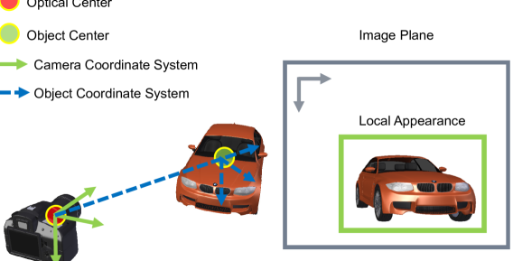
Previous studies [71, 21, 40, 81] regress vehicle orientation with the computational graph in Eq. 1. A CNN-based model $\mathcal{N}$ is used to map local instance appearance $\mathbf{x}_{i}$ to allocentric pose, i.e., 3D orientation in the object coordinate system (OCS), which is then converted to the egocentric pose, i.e., orientation in the camera coordinate system (CCS). The difference between these two coordinate systems is shown in Fig. 5. This two-step design is a workaround since an object with the same egocentric pose $\bm{\theta}_{i}$ can produce different local appearance depending on its location [21] and learning the mapping from $\mathbf{x}_{i}$ to $\bm{\theta}_{i}$ is ill-posed. In this two-step design, OCS was estimated by another module. The error of this module can propagate to the final estimation of egocentric poses and optimizing $\mathcal{N}$ does not optimize the final target directly. Another problem of this design is that the mapping from pixels $\mathbf{x}_{i}$ to pose vectors $\bm{\alpha}_{i}$ is highly non-linear and difficult to approximate [82].

$$\begin{array}[]{llll}\mathbf{x}_{i}&\xrightarrow{\mathcal{N}}&~{}~{}\bm{\alpha}_{i}&\xrightarrow{convert}~{}~{}\bm{\theta}_{i}\\ &&\text{OCS}&\nearrow{}\\ \end{array}$$ (1)

Figure 5: Local appearance cannot uniquely determine egocentric pose. Existing solutions first estimate allocentric pose in the object coordinate system (blue) and convert it to egocentric pose in the camera coordinate system (green) based on the object location.

Ego-Net instead learns a mapping from images to egocentric poses to optimize the target directly. However, instead of relying on a black box model to fit such a non-linear mapping, it promotes a progressive mapping, where coordinate-based IGRs are extracted from pixels and eventually lifted to the 3D target. Specifically, Ego-Net is a composite function with learnable modules $\{\mathcal{H},\mathcal{C},Li\}$. Given the cropped 2D image patch of one proposal $\mathbf{x}_{i}$, Ego-Net predicts its egocentric pose as $\mathcal{E}(\mathbf{x}_{i})=Li(\mathcal{A}_{i}(\mathcal{C}(\mathcal{H}(\mathbf{x}_{i}))))=\bm{\theta}_{i}$. Fig. 3 depicts Ego-Net, whose computational graph is shown in Eq. 2. $\mathcal{H}$ extracts heatmaps $h(\mathbf{x}_{i})$ for 2D object parts that are mapped by $\mathcal{C}$ to coordinates $\phi_{l}(\mathbf{x}_{i})$ representing their local location on the patch. $\phi_{l}(\mathbf{x}_{i})$ is converted to the global image plane coordinates $\phi_{g}(\mathbf{x}_{i})$ with an affine transformation $\mathcal{A}_{i}$ parametrized with scaling and 2D translation. $\phi_{g}(\mathbf{x}_{i})$ is further lifted to a 3D representation $\psi(\mathbf{x}_{i})$ by $Li$. The final pose prediction derives from $\psi(\mathbf{x}_{i})$.

$$\begin{array}[]{lllllllllll}\mathbf{x}_{i}&\xrightarrow{\mathcal{H}}&h(\mathbf{x}_{i})&\xrightarrow{\mathcal{C}}&\phi_{l}(\mathbf{x}_{i})&\xrightarrow{\mathcal{A}_{i}}&\phi_{g}(\mathbf{x}_{i})&\xrightarrow{Li}&\psi(\mathbf{x}_{i})&\rightarrow&\bm{\theta}_{i}\end{array}$$ (2)

IV-B Design of Labor-free Intermediate Representations

The IGRs in Eq. 2 are designed considering:

Availability: It is favorable if the IGRs can be easily derived from existing ground truth annotations with none or minimum extra manual effort. Thus we define object parts from existing 3D bounding box annotations.

Discriminative: The IGRs should be indicative for orientation estimation, so that they can serve as a good bridge between visual appearance input and the geometrical target.

Transparency: The IGRs should be easy to understand, which makes them debugging-friendly and trustworthy for applications such as autonomous driving. Thus IGRs are defined with explicit meaning in Ego-Net.

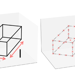
With the above considerations, we define the 3D representation $\psi(\mathbf{x}_{i})$ as a sparse 3D point cloud (PC) representing an interpolated cuboid. Autonomous driving datasets such as KITTI [83] usually label instance 3D bounding boxes from captured point clouds where an instance $\mathbf{x}_{i}$ is associated with its centroid location in the camera coordinate system $\mathbf{t}_{i}=[t_{x},t_{y},t_{z}]$, size $[h_{i},w_{i},l_{i}]$, and its egocentric pose $\bm{\theta}_{i}$. For consistency, many prior studies only use the yaw angle denoted as $\theta_{i}$. As shown in Fig. 6, denote the 12 lines enclosing the vehicle as $\{\mathbf{l}_{j}\}_{j=1}^{12}$, where each line is represented by two endpoints (start and end) as $\mathbf{l}_{j}=[\mathbf{p}_{j}^{s};\mathbf{p}_{j}^{e}]$. $\mathbf{p}_{j}^{v}$ ($v$ is $s$ or $e$) is a 3-vector $(X_{j}^{v},Y_{j}^{v},Z_{j}^{v})$ representing the point’s location in the camera coordinate system. As a complexity-controlling parameter, $q$ more points are derived from each line with a pre-defined interpolation matrix $B_{q\times 2}$ as

$$\begin{bmatrix}\mathbf{p}_{j}^{1}\\ \mathbf{p}_{j}^{2}\\ \dots\\ \mathbf{p}_{j}^{q}\\ \end{bmatrix}=B_{q\times 2}\begin{bmatrix}\mathbf{p}_{j}^{s}\\ \mathbf{p}_{j}^{e}\\ \end{bmatrix}=\begin{bmatrix}\beta_{1}&1-\beta_{1}\\ \beta_{2}&1-\beta_{2}\\ \dots&\dots\\ \beta_{q}&1-\beta_{q}\\ \end{bmatrix}\begin{bmatrix}\mathbf{p}_{j}^{s}\\ \mathbf{p}_{j}^{e}\\ \end{bmatrix}.$$ (3)

The 8 endpoints, the instance’s centroid, and the interpolated points for each of the 12 lines form a set of $9+12q$ points. The concatenation of these points forms a $9+12q$ by $3$ matrix $\tau(\mathbf{x}_{i})$. Since we do not need the 3D target $\psi(\mathbf{x}_{i})$ to encode location, we deduct the instance translation $\mathbf{t}_{i}$ from $\tau(\mathbf{x}_{i})$ and represent $\psi(\mathbf{x}_{i})$ as a set of $8+12q$ points representing the shape relative to the centroid $\psi(\mathbf{x}_{i})=\{(X_{j}^{v}-t_{x},Y_{j}^{v}-t_{y},Z_{j}^{v}-t_{z})\}$ where $v\in\{s,1,\dots,q,e\}$ and $j\in\{1,2,\dots,12\}$. Larger $q$ provides more cues for inferring pose yet increases complexity. In practice we choose $q=2$ and the right figure of Fig. 6 shows an example with $B_{2\times 2}=\begin{bmatrix}\frac{3}{4}&\frac{1}{4}\\ \frac{1}{4}&\frac{3}{4}\\ \end{bmatrix}$ and 2 points are interpolated for each line.

Serving as the 2D representation to be located by $\mathcal{H}$ and $\mathcal{C}$, $\phi_{g}(\mathbf{x}_{i})$ is defined to be the projected screen coordinates of $\tau(\mathbf{x}_{i})$ given camera intrinsics $\text{K}_{3\times 3}$ as

$$\phi_{g}(\mathbf{x}_{i})=\text{K}_{3\times 3}\tau(\mathbf{x}_{i}).$$ (4)

Figure 6: An instance $\mathbf{x}_{i}$ with primitive 3D bounding box annotation (left) and its 3D point cloud representation $\psi(\mathbf{x}_{i})$ (right) in the camera coordinate system as the collection of red crosses.

$\phi_{g}(\mathbf{x}_{i})$ implicitly encodes instance location on the image plane so that it is not an ill-posed problem to estimate egocentric pose from it directly. In summary, these IGRs can be computed with zero extra manual annotation, are easy to understand, and contain rich information for estimating the instance orientation.

V Ego-Net++: towards multi-view perception and implicit shape inference

V-A Orientation estimation with paired part coordinates

Under the stereo perception setting, another viewpoint provides more information to infer the unknown object orientation. It is thus necessary to extend the IGRs to aggregate information from both views.

Figure 7: Diagram of the paired part coordinates representation for an object part (red) of a non-rigid object.

Figure 8: Zoomed-in view of the orientation estimation part in $\mathcal{E}$ in Fig. 4.

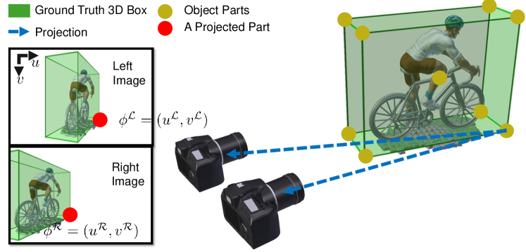
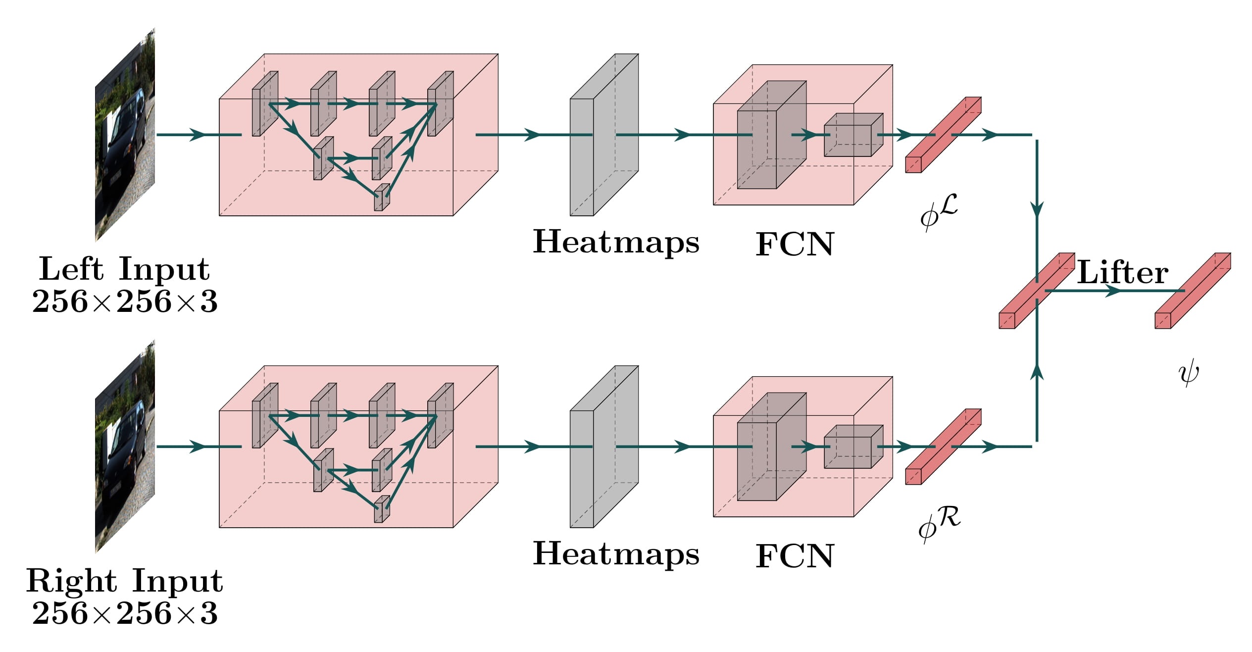
In Ego-Net++, paired part coordinates (PPCs) are defined with a simple-yet-effective concatenation operation to aggregate two-view information as a k by 4 representation

$$\phi_{g}(\mathbf{x}_{i}^{\mathcal{L}},\mathbf{x}_{i}^{\mathcal{R}})=\phi_{g}(\mathbf{x}_{i}^{\mathcal{L}})\oplus\phi_{g}(\mathbf{x}_{i}^{\mathcal{R}}),$$ (5)

PPC is illustrated in Fig. 7. for one object part, and it extends the computational graph in Eq. 2 as

The learnable modules are implemented with convolutional and fully-connected layers. During training, ground truth IGRs are available to penalize the predicted heatmaps, predicted 2D coordinates, and 3D coordinates. Such supervision is implemented with $L_{2}$ loss for heatmaps and $L_{1}$ loss for coordinates. In inference, the predicted egocentric pose is obtained by estimating the rotation from an interpolated cuboid at a canonical pose to the predicted 3D coordinates, which is solved efficiently with SVD.

V-B Implicit shape reconstruction via surface hallucination

Previous sections enable recovering object orientation from one or two views. However, such perception capability is limited to describing objects as 3D bounding boxes, failing at a more detailed representation within the box. While some previous studies [31, 32, 23, 34] explore shape estimation for outdoor rigid objects, they cannot exploit the stereo inputs or require PCA-based templates [31, 32, 23, 34] which are limited to a fixed mesh topology [23]. In contrast, this study can take advantage of stereo information and conduct implicit shape estimation which can produce flexible resolution-agnostic meshes. To our best knowledge, how to design effective intermediate representations for recovering implicit shape attributes for outdoor rigid objects with stereo cameras is under-explored.

We design the IGRs for implicit shape estimation based on the following fact. The implicit shape representation $s(\mathbf{x}_{i})$ for each rigid object describes its complete surface geometry. However, the observation from stereo cameras only encodes a portion of the object’s surface. This indicates that the implicit shape reconstruction problem can be modeled as a unseen surface hallucination problem, i.e., one needs to infer the unseen surface based on partial visual evidence. Specifically, Ego-Net++ addresses this problem by extending the IGRs in Ego-Net with several new representations and learning a progressive mapping from stereo appearances to $s(\mathbf{x}_{i})$. This mapping is represented as a composite function $E\circ Ha\circ O\circ V,$ that has learnable parameters $\{Ha,V,E\}$ and the following computational graph

$$\begin{array}[]{lllllllll}\mathbf{x}_{i}^{\mathcal{L}},\mathbf{x}_{i}^{\mathcal{R}}&\xrightarrow{V}&v(\mathbf{x}_{i})&\xrightarrow{O}&o(\mathbf{x}_{i})&\xrightarrow{Ha}&ha(\mathbf{x}_{i})&\xrightarrow{E}&s(\mathbf{x}_{i}).\end{array}$$ (7)

Here $v(\mathbf{x}_{i})$ represents the visible portion of the object surface. After a normalization operator, such representation is converted to the OCS. To recover the missing surface, a point-based encoder-decoder $Ha$ hallucinates a complete surface based on learned prior knowledge of an object class. $E$ encodes the complete shape into an implicit shape vector.

V-C The visible-surface representation

We propose a point-based representation for the visible object surface. Given a pair of stereo RoIs, $V$ estimates the foreground mask and depth, samples a set of pixels from the foreground, and re-projects them to the CCS. Denote $\mathcal{M}(\mathbf{x}_{i})$ as the predicted set of foreground pixels, we sample $e$ elements from it as $\mathcal{M}^{sp}(\mathbf{x}_{i})$. These elements are re-projected to the CCS to form a set of $e$ 3D points as

$$\{\text{K}_{3\times 3}^{-1}\begin{bmatrix}w_{m}*m^{x}\\ w_{m}*m^{y}\\ w_{m}\\ \end{bmatrix}|m\in\mathcal{M}^{sp}(\mathbf{x}_{i})\subset\mathcal{M}(\mathbf{x}_{i})\},$$ (8)

where $(m^{x},m^{y})$ denotes the screen coordinates of pixel $m$. Concatenating these elements gives a 3 by $e$ matrix $v(\mathbf{x}_{i})$ encoding the visible instance PC in the CCS.

In implementation, $\mathcal{M}(\mathbf{x}_{i})$ is obtained by a fully convolutional network that uses 2D features for foreground classification. To obtain the depth prediction for the foreground region, a local cost volume is constructed to estimate disparity for the local patch. The disparities are then converted to depth as $m^{z}=fB/m^{disp}$ where $m^{disp}$, $B$, and $f$ are the estimated disparity, stereo baseline length, and focal length respectively.

V-D Hallucination with normalized points

To ease the learning of unseen surface hallucination conditioned on the visible surface, the operator $O$ normalizes the visible PC to the canonical OCS conditioned on the current bounding box prediction $b_{i}$ as

$$o(\mathbf{x}_{i})=\begin{gathered}\begin{bmatrix}cos\theta_{i}*l_{i}&0&sin\theta_{i}*l_{i}&t_{x}\\ 0&l_{i}&0&t_{y}\\ -sin\theta_{i}*l_{i}&0&cos\theta_{i}*l_{i}&t_{z}\\ 0&0&0&1\end{bmatrix}^{-1}\begin{bmatrix}\vline\\ v(\mathbf{x}_{i})\\ \vline\\ \textbf{1}\end{bmatrix}.\end{gathered}$$ (9)

$Ha$ is implemented as a point-based encoder-decoder module, which extracts point-level features [84] from $o(\mathbf{x}_{i})$ and infers $N_{c}$ by 3 coordinates to represent the complete surface.

Finally, the shape encoder $E$ maps the estimated complete surface $c(\mathbf{x}_{i})$ into a latent vector $s(\mathbf{x}_{i})$ that encodes the object’s implicit shape.

To extract a mesh representation from the predicted implicit shape code, $\mathcal{E}$ uses the occupancy decoder [77] where a set of grid locations is specified and predicts the occupancy field on such grid. Note this grid is not necessarily evenly distributed thus one can easily use the shape code in a resolution-agnostic manner. Given the occupancy field, we then use the Marching Cube algorithm [85] to extract an isosurface as a mesh representation.

To optimize the parameters in the above-mentioned modules during training, the supervision consists of the cross-entropy segmentation loss, the smooth $L_{1}$ disparity estimation loss, and the hallucination loss implemented as Chamfer distance. We train the shape decoder on ShapeNet [86] by randomly sampling grid locations within object 3D bounding boxes with paired ground truth occupancy. In inference, we apply zero padding if $Card(\mathcal{M}(\mathbf{x}_{i}))<e$.

V-E Penalizing in-box descriptions for 3D object detection

Per the new representations introduced in Ego-Net++, S-3D-RCNN can not only estimate 3D bounding boxes accurately from stereo cameras but also can describe detected rigid objects within the bounding boxes. However, existing 3DOD studies only penalize the predicted 3D bounding boxes and fail to measure the goodness of a more detailed representation within the boxes. To fill this gap, we extend the previous official metrics to enable them for the required evaluation.

As a basic metric to extend, the official Average Orientation Similarity ($AOS$) metric in KITTI is defined as

$$AOS=\frac{1}{11}\sum_{r\in\{0,0.1,\dots,1\}}\text{max}_{\tilde{r}:\tilde{r}\geq r}s(\tilde{r}),$$ (10)

where $r$ is the detection recall and $s(r)\in[0,1]$ is the orientation similarity (OS) at recall level $r$. OS is defined as

$$s(r)=\frac{1}{|D(r)|}\sum_{b_{i}\in D(r)}\frac{1+\text{cos}\Delta_{i}^{\theta}}{2}\delta_{i}$$ (11)

, where $D(r)$ denotes the set of all object predictions at recall rate $r$ and $\Delta^{(i)}_{\theta}$ is the difference in yaw angle between estimated and ground-truth orientation for object $i$. If $b_{i}$ is a 2D false positive, i.e., its 2D intersection-over-union (IoU) with ground truth is smaller than a threshold (0.5 or 0.7), $\delta_{i}=0$. Note that $AOS$ itself builds on the official average precision metric $AP_{2D}$ and is upper-bounded by $AP_{2D}$. $AOS=AP_{2D}$ if and only if there is no false-positive prediction and the orientation estimations are perfect.

Based on Minimal Matching Distance (MMD)[87, 88], we propose a new metric $AP_{MMD}$ in the same manner as

$$AP_{MMD}=\frac{1}{11}\sum_{r\in\{0,0.1,\dots,1\}}\text{max}_{\tilde{r}:\tilde{r}\geq r}s_{MMD}(\tilde{r})$$ (12)

where $r$ is the same detection recall and $s_{MMD}(r)\in[0,1]$ is the MMD similarity (MMDS) at recall level $r$. MMDS is defined as

$$s_{MMD}(r)=\frac{1}{|D(r)|}\sum_{b_{i}\in D(r)}[(0.05-MMD(c(\mathbf{x}_{i}))*20]\delta_{i}^{MMD}$$ (13)

, where $\delta_{i}^{MMD}$ is a indicator and $MMD(c(\mathbf{x}_{i}))$ denotes the MMD of prediction $i$ which measures the quality of the predicted surface. If the $i$th prediction is a false postive or $MMD(c(\mathbf{x}_{i}))>0.05$, $\delta_{i}^{MMD}=0$. $AP_{MMD}$ is thus also upper-bounded by the official $AP_{2D}$. $AP_{MMD}=AP_{2D}$ if and only if there is no false positive prediction and $MMD(c(\mathbf{x}_{i}))=0$ for all predictions.

Since instance-level ground truth shape is not available in KITTI, $MMD(c(\mathbf{x}_{i}))$ is implemented as category-level similarity similar to [87, 88]. For a predicted instance PC $c(\mathbf{x}_{i})$, it is defined as the minimal $L_{2}$ Chamfer distance between it and a collection of template PCs in ShapeNet [86] that has the same class label. It is formally expressed as $MMD(c(\mathbf{x}_{i}))=\min_{\mathcal{G}\in SN}d_{CD}(c(\mathbf{x}_{i}),\mathcal{G}),$ where $SN$ stands for the set of ShapeNet template PCs and $d_{CD}(c(\mathbf{x}_{i}),\mathcal{G})$ is defined as

During the evaluation, we downloaded 250 ground truth car PCs that were used in [87, 88] for consistency.

$AP_{MMD}$ penalizes all predictions including false negatives. For completeness, we propose True Positive Minimal Matching Distance (MMDTP) to evaluate MMD for true positive predictions similar to [89]. We define MMDTP@$\beta$ as the average MMD of the predicted objects that have 3D IoU $>$ $\beta$ with at least one ground truth object,

$$MMDTP@\beta=\frac{1}{SUM}\sum_{i=1}^{N}TP(i)*MMD(c(\mathbf{x}_{i})),$$ (15)

where $TP(i)$ is 1 if $b_{i}$ is a true positive and 0 otherwise as

$$TP(i)=\begin{cases}1,&\mbox{if }IoU_{3D}(b_{i},gt)>\beta,\exists gt\\ 0,&\mbox{else}.\end{cases}$$

and $SUM=\sum_{i=1}^{N}TP(i)$.

VI Experiments

We first introduce the used benchmark dataset and the evaluation metrics, followed by a system-level comparison between our S-3D-RCNN with other approaches in terms of outdoor 3D scene understanding capabilities. We further present a module-level comparison to demonstrate the effectiveness of the proposed IGRs in Ego-Net++. Finally, we conduct an ablation study on key design factors and hyper-parameters.

VI-A Experimental settings

Dataset. We employ the KITTI object detection benchmark [83] that contains stereo RGB images captured in outdoor scenes. The dataset is split into 7,481 training images and 7,518 testing images. The training images are further split into the train split and the val split containing 3,712 and 3,769 images respectively. For consistency with prior studies, we use the train split for training and report results on the val split and the testing images.

Evaluation metrics. We use the official average precision metrics as well as our newly designed $AP_{MMD}$ and MMDTP. As defined in Eq. 10, $AOS$ is used to assess the system performance for joint object detection and orientation estimation. 3D Average Precision ($AP_{3D}$) measures precisions at the same recall values where a true positive prediction has 3D IoU $>$ 0.7 with the ground truth one. BEV Average Precision ($AP_{BEV}$) instead uses 2D IoU $>$ 0.7 as the criterion for true positives where the 3D bounding boxes are projected to the ground plane. Each ground truth label is assigned a difficulty level (easy, moderate, or hard) depending on its 2D bounding box height, occlusion level, and truncation level.

Method	Reference	Modality	Number of Viewpoints	Easy	Moderate	Hard	Average
Mono3D [90]	CVPR’ 16	RGB	Monocular	91.01	86.62	76.84	84.82
Deep3DBox [71]	CVPR’ 17	RGB	Monocular	92.90	88.75	76.76	86.14
ML-Fusion [91]	CVPR’ 18	RGB	Monocular	90.35	87.03	76.37	84.58
FQNet [73]	CVPR’ 19	RGB	Monocular	92.58	88.72	76.85	86.05
GS3D [92]	CVPR’ 19	RGB	Monocular	85.79	75.63	61.85	74.42
MonoPSR [93]	CVPR’ 19	RGB + LiDAR	Monocular	93.29	87.45	72.26	84.33
M3D-RPN [40]	ICCV’ 19	RGB	Monocular	88.38	82.81	67.08	79.42
MonoPair [94]	CVPR’ 20	RGB	Monocular	91.65	86.11	76.45	84.74
Disp R-CNN [43]	CVPR’ 20	RGB + LiDAR	Stereo	93.02	81.70	67.16	80.63
DSGN [33]	CVPR’ 20	RGB	Stereo	95.42	86.03	78.27	86.57
D4LCN [81]	CVPR’ 20	RGB	Monocular	90.01	82.08	63.98	78.69
RAR-Net [75]	ECCV’ 20	RGB	Monocular	88.40	82.63	66.90	79.31
RTM3D [95]	ECCV’ 20	RGB	Monocular	91.75	86.73	77.18	85.22
Kinematic3D [96]	ECCV’ 20	RGB	Monocular	58.33	45.50	34.81	46.21
Ours [2]	CVPR’ 21	RGB	Monocular	96.11	91.23	80.96	89.43

TABLE I: System-level evaluation by comparing Average Orientation Similarity ($AOS$) with previous learning-based methods on the KITTI test set for the car category. Without using LiDAR data [93] during training (indicated by +LiDAR) or temporal information [96], a monocular system using Ego-Net out-performs previous image-based methods.

Method	Reference	Modality	Number of Viewpoints	Easy	Moderate	Hard	Average
PointPillars [97]	CVPR’ 19	LiDAR	N/A	57.47	48.05	45.40	50.31
PointRCNN [54]	CVPR’ 19	LiDAR	N/A	57.19	47.33	44.31	49.61
M3D-RPN [40]	ICCV’ 19	RGB	Monocular	44.33	31.88	28.55	34.92
TANet [98]	AAAI’ 20	LiDAR	N/A	42.54	36.21	34.39	37.71
Disp R-CNN [43]	CVPR’ 20	RGB + LiDAR	Stereo	63.16	45.66	41.14	50.00
D4LCN [81]	CVPR’ 20	RGB	Monocular	46.73	33.62	28.71	36.35
DSGN [33]	CVPR’ 20	RGB	Stereo	31.21	24.32	23.09	26.21
YOLOStereo [99]	ICRA’ 21	RGB	Stereo	48.99	35.62	31.58	38.73
MonoEF [100]	CVPR’ 21	RGB	Monocular	47.45	34.63	31.01	37.70
CaDDN [45]	CVPR’21	RGB	Monocular	24.45	17.13	15.79	19.12
LIGA-Stereo [49]	ICCV’ 21	RGB + LiDAR	Stereo	53.16	40.98	38.12	44.09
GUPNet [101]	ICCV’ 21	RGB	Monocular	68.93	50.74	44.01	54.56
MonoCon [102]	AAAI’ 22	RGB	Monocular	52.16	38.67	33.15	41.33
Ours	N/A	RGB	Stereo	73.14	53.92	46.93	57.98

TABLE II: Comparison of $AOS$ with other methods on the KITTI test set for the pedestrian category. Without using LiDAR data [97], a stereo system using Ego-Net++ significantly outperforms previous studies. The proposals are the same as GUPNet [101].

Figure 9: Qualitative results of S-3D-RCNN on KITTI val set. Left: input left images and 3D proposals. Middle: rendered objects in the original camera view. Right: rendered objects in a different view (camera 2 meters higher with 15^∘ pitch angle).

Qualitative comparison of perception capability
Method	Modality	Location	Dimension	Orientation	Shape Representation
					Instance point cloud	Mesh	Implicit shape
3D-RCNN [21]	Monocular	✓	✓	✓		✓
DSGN [33]	Stereo	✓	✓	✓	✓ (Partial)
Disp-RCNN [43]	Stereo	✓	✓	✓	✓ (Partial)
S-3D-RCNN (Ours)	Stereo	✓	✓	✓	✓ (Full)	✓	✓
Quantitative comparison of 3D object detection performance
Method		$AP_{3D}@R_{11}\uparrow$			$AP_{BEV}@R_{11}\uparrow$
		Easy	Moderate	Hard	Easy	Moderate	Hard
3D-RCNN [21]		N/A	N/A	N/A	N/A	N/A	N/A
DSGN [33]		72.31	54.27	47.71	83.24	63.91	57.83
Disp-RCNN [43]		64.29	47.73	40.11	77.63	64.38	50.68
S-3D-RCNN (Ours)		77.04	62.98	56.56	87.37	72.87	66.62
Quantitative comparison of shape reconstruction performance with MMDTP@0.5$\downarrow$
Depth range		(0,10m]	(10,20m]	(20,30m]	(30,40m]	(40,50m]	(50,60m]
DSGN [33]		0.036	0.039	0.041	0.044	0.048	0.051
Disp-RCNN [43]		0.034	0.037	0.039	0.038	0.041	0.034
Disp-RCNN [43]+ $\mathcal{E}$		0.0051	0.0071	0.0074	0.0065	0.0050	0.0035

TABLE III: A comparison of image-based outdoor 3D scene understanding performance on the KITTI val set for the Car class. We compare with methods that can perform 3D object localization as well as provide at least one type of object shape representation. During evaluating MMDTP, the predictions are grouped according to the predicted depth.

VI-B System-level comparison with previous studies

VI-B1 Joint object detection and orientation estimation performance

Ego-Net can be used with a 2D proposal model to form a joint object detection and orientation estimation system, whose performance is measured by $AOS$. Per the proposals used in [2], Tab. I compares the $AOS$ of our system using Ego-Net with other approaches on the KITTI test set for the car category. Among the single-view image-based approaches, our system outperforms others by a clear margin. Our approach using a single image outperforms Kinematic3D [96] which exploits temporal information using RGB video. This result indicates that vehicle pose can be reliably estimated with a single frame. In fact, our approach can also serve for per-frame initialization of temporal models.

In addition to orientation estimation for rigid objects with monocular images, we provide extended studies and performance comparison in Tab. II for the pedestrian class with our Ego-Net++ that uses stereo images. For a fair comparison, we use the same proposals in [101]. Using our $\mathcal{E}$ consistently outperforms the proposal model and the system performance based on RGB images even surpasses some LiDAR-based approaches [97, 54] that have more accurate depth measurements. This result indicates that the LiDAR point cloud is not discriminative for determining the accurate orientation of distant non-rigid objects due to a lack of fine-grained visual information. In contrast, our image-based approach effectively addresses the limitations of LiDAR sensors and can complement them in this scenario.

VI-B2 Comparison of 3D scene understanding capability

To our best knowledge, S-3D-RCNN is the first model that jointly performs accurate 3DOD and implicit shape estimation for outdoor rigid objects with stereo cameras. Tab. III presents a summary and comparison of perception capability with previous image-based outdoor 3D scene understanding approaches. Qualitatively, S-3D-RCNN is the only method that can utilize stereo geometry as well as predict implicit shape representations. Compared to the monocular method 3D-RCNN [21] that uses template meshes with fixed topology, our framework can produce meshes in a resolution-agnostic way and can provide an accurate estimation of object locations by exploiting two-view geometry. We show qualitative results in Fig. 9 where the predicted implicit shapes are decoded to meshes. Our approach shows accurate localization performance along with plausible shape predictions, which opens up new opportunities for outdoor augmented reality.

VI-C Module-level comparison with previous studies

VI-C1 Comparison of orientation estimation performance

To assess if Ego-Net can help improve the pose estimation accuracy of other 3DOD systems, we download proposals from other open-source implementations and use Ego-Net for orientation refinement. The result is summarized in Tab. IV for the car category. While $AOS$ depends on the detection performance of these methods, using Ego-Net consistently improves the pose estimation accuracy of these approaches. This indicates that Ego-Net is robust despite the performance of a vehicle detector varying with different recall levels. For true positive predictions we plot the distribution of orientation estimation error versus different depth ranges and occlusion levels in Fig. 10. The error in each bin is the averaged orientation estimation error for those instances that fall into it. While the performance of M3D-RPN [40] and D4LCN [81] degrades significantly for distant and occluded cars, the errors of our approach increase gracefully. We believe that explicitly learning the object parts makes our model more robust to occlusion as the visible parts can provide rich information for pose estimation.

Method	$AOS\&AP_{2D}$,  $AOS\leq AP_{2D}$
	Easy	Moderate	Hard
	$AP_{2D}$
M3D-RPN [40]	90.28	83.75	67.72
D4LCN [81]	92.80	84.43	67.89
Method	$AOS$
M3D-RPN [40]	88.79	81.25	65.37
M3D-RPN + Ego-Net	90.20	83.60	67.53
D4LCN [81]	91.74	82.96	66.45
D4LCN + OCM3D [103]	92.12	83.27	66.81
D4LCN + Ego-Net	92.62	84.25	67.60

TABLE IV: $AOS$ evaluation on KITTI validation set. After employing Ego-Net, the vehicle pose estimation accuracy of other 3DOD systems can be improved. The space for $AOS$ improvement is upper-bounded by $AP_{2D}$.

Figure 10: Average orientation error (AOE) on KITTI val split in different depth ranges and occlusion levels. Our approach is robust to distant and partially occluded instances.

Figure 11: Detected instances on KITTI val split along with the comparison of the predicted vehicle orientations in bird’s eye view.

Figure 12: Similar comparison as Fig. 11 showing pedestrian orientation predictions using two-view images as inputs.

Method	$AP_{BEV}$
	Easy	Moderate	Hard
ROI-10D [104]	14.04	3.69	3.56
Mono3D++ [105]	16.70	11.50	10.10
MonoDIS [41]	24.26	18.43	16.95
D4LCN [81]	31.53	22.58	17.87
D4LCN + Ego-Net (Ours)	33.60	25.38	22.80

TABLE V: $AP_{BEV}$ evaluated on KITTI validation set. Ego-Net can correct the erroneous pose predictions from [81] as shown in Fig. 11.

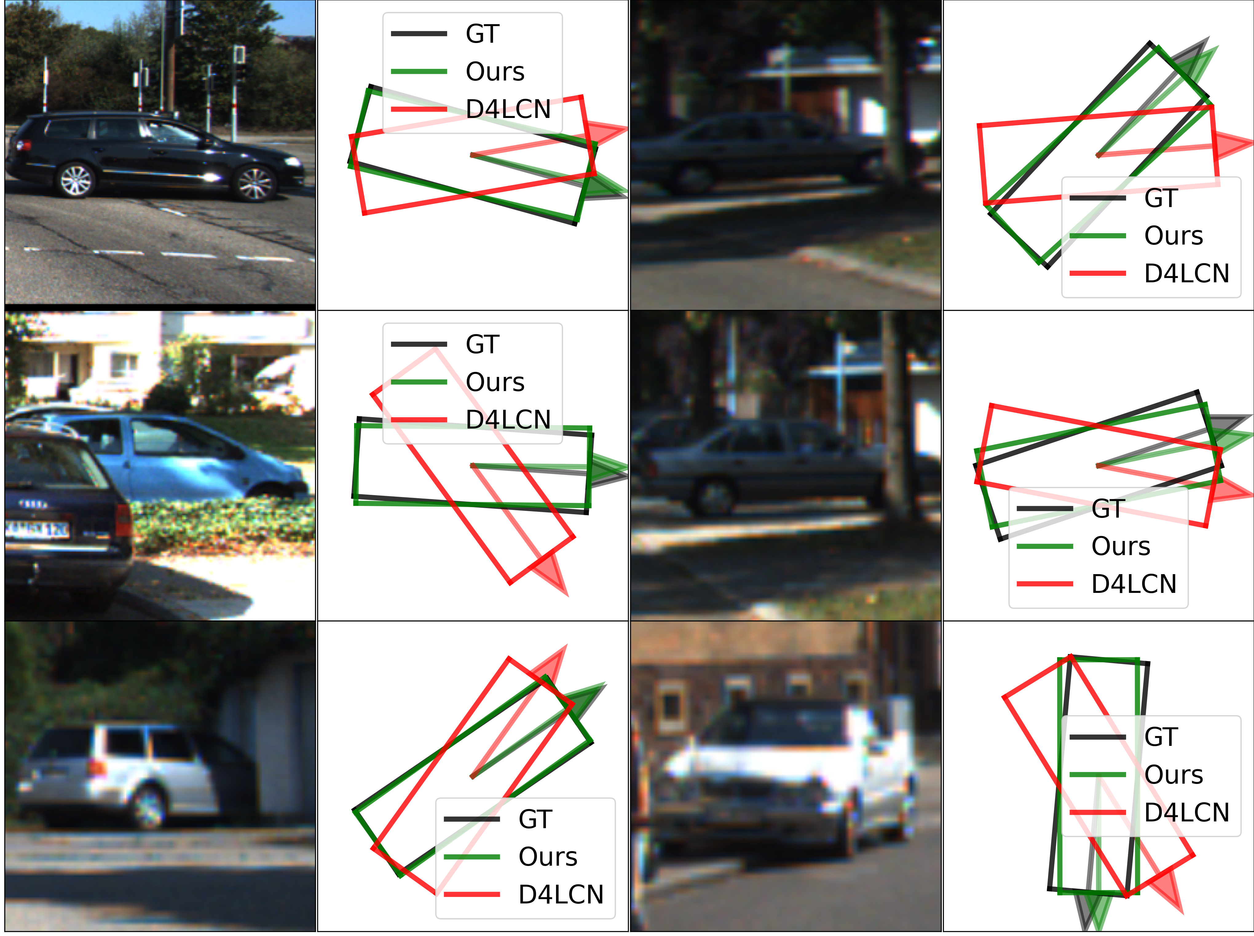
Bird’s eye view (BEV) evaluation compared with D4LCN [81] is visualized in Fig. 11. The orientation predictions are shown in BEV and the arrows point to the heading direction of those vehicles. From the local appearance, it can be hard to tell whether certain cars head towards or away from the camera, as validated by the erroneous predictions of D4LCN [81] since it regresses pose from local features. In comparison, our approach gives accurate egocentric pose predictions for these instances and others that are partially occluded. Quantitative comparison with several 3D object detection systems on the KITTI val split is shown in Tab. V. Note that utilizing Ego-Net can correct wrong pose predictions especially for difficult instances, which leads to improved 3D IoU and results in significantly improved $AP_{BEV}$.

Method	$AP_{3D}@R_{40}$
	Easy	Moderate	Hard
LIGA [49]	45.54	37.80	32.09
LIGA + Ego-Net++ (Ours)	50.25	44.48	38.63
Method	$AP_{BEV}@R_{40}$
	Easy	Moderate	Hard
LIGA [49]	54.59	47.14	41.12
LIGA + Ego-Net++ (Ours)	59.55	53.35	47.96
Method	$AOS@R_{40}$
	Easy	Moderate	Hard
LIGA [49]	54.64	48.22	43.10
LIGA + Ego-Net++ (Ours)	73.56	69.28	62.92

TABLE VI: Quantitative comparison for orientation predictions for pedestrians on the KITTI val set using the same proposals as [49]. 40 recall values are used for consistency.

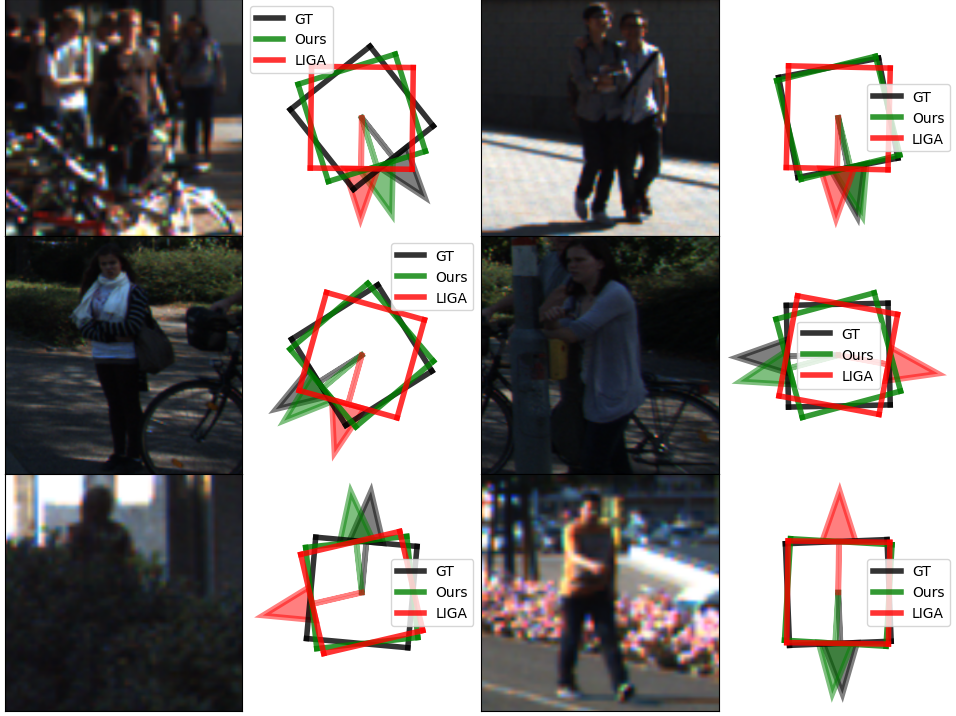
Apart from using Ego-Net for monocular detectors, we also provide extended studies of using Ego-Net++ for stereo detectors. Tab.VI instead shows a comparison for the non-rigid pedestrian class where the same proposals are used as a stereo 3D object detector [49]. Thanks to the effectiveness of PPC, our $\mathcal{E}$ significantly improves the 3DOD performance for these non-rigid objects and some examples are shown in Fig. 12.

Figure 13: Qualitative comparison for instances on the KITTI val split. Left: instance RoIs in the left image. Middle: instance point cloud predictions from Disp R-CNN [43]. Right: Our predictions $c(\mathbf{x}_{i})$ after the hallucination module.

Figure 14: The bar plots show the distribution of the predicted bounding boxes used in MMDTP evaluation. The average MMD for each bin is shown in the line plots. Using $\mathcal{E}$ consistently improves performance for objects in all bins.

VI-C2 Comparison of shape estimation performance

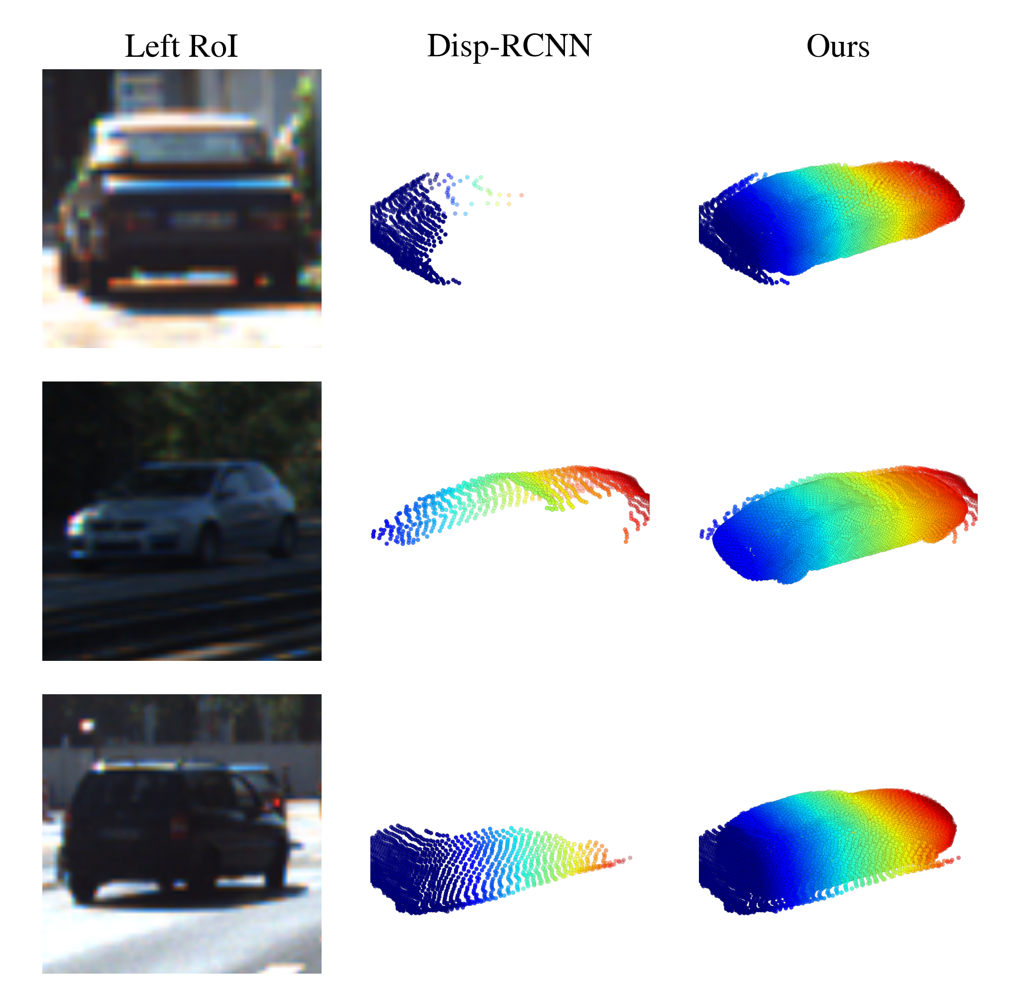
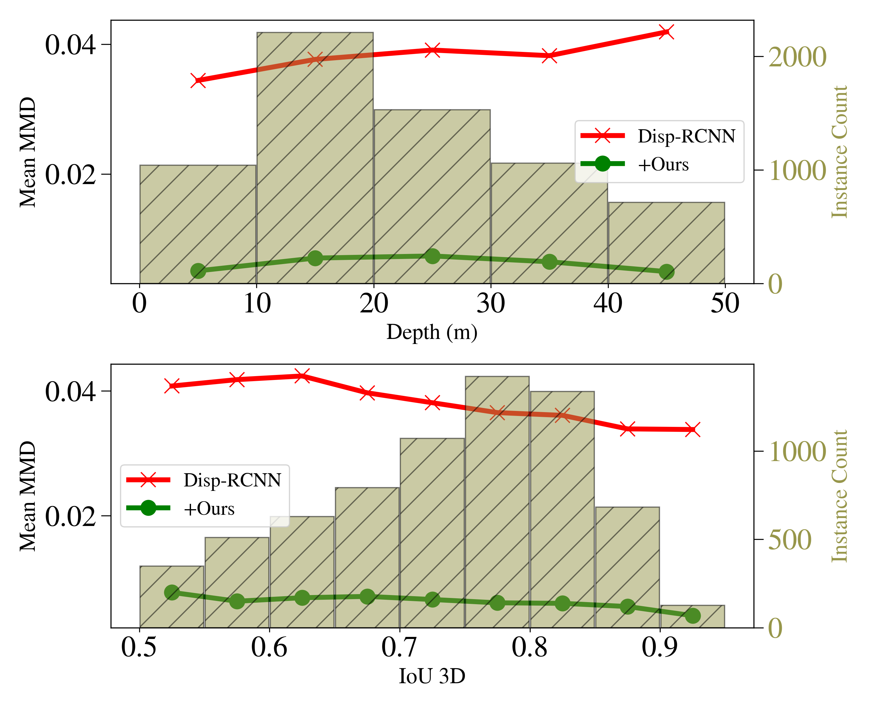
Here we present a quantitative comparison of shape estimation quality using our newly-introduced metric MMDTP. We compare with [43] for MMDTP due to its availability of the official implementation. We downloaded 13,575 predicted objects from its website in which 9,488 instances have 3D IoU large enough to compute MMDTP@0.5 shown in Tab. III. Our $\mathcal{E}$ can produce a complete shape description of a detected instance thanks to our visible surface representation and explicit modeling of the unseen surface hallucination problem. This leads to a significant improvement in MMDTP. Fig. 13 shows a qualitative comparison of the predicted instance shapes as PCs. Note that the visible portion of the instances varies from one to another, but our $\mathcal{E}$ can reliably infer the invisible surface. Fig. 14 shows the relationship between MMDTP with factors such as object depth and bounding box quality. More distant objects and less accurate 3D bounding boxes suffer from larger MMD for [43] due to fewer visible points and larger alignment errors. Note that our approach consistently improves [43] across different depth ranges and box proposal quality levels.

Method	Reference	$AP_{MMD}@R_{11}$ (2D IoU $>$ 0.7)			$AP_{MMD}@R_{11}$ (2D IoU $>$ 0.5)
		Easy	Moderate	Hard	Easy	Moderate	Hard
Disp-RCNN [43]	CVPR’ 20	37.50	30.93	25.29	37.66	31.34	26.68
Disp-RCNN + $\mathcal{E}$ (Ours)	N/A	89.10	83.71	72.26	89.56	84.90	77.13

TABLE VII: Quantitative comparison using our introduced new metric $AP_{MMD}$ on KITTI val split.

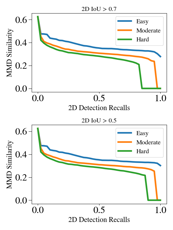
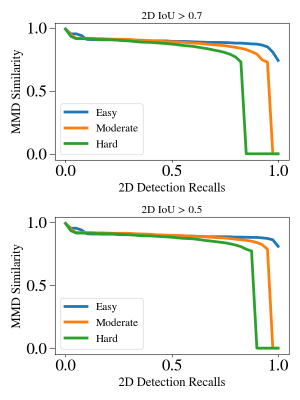
Per our definition of $AP_{MMD}$, the $s_{MMD}$ at different recall values are shown in Fig. 15 for the predictions of Disp-RCNN. In contrast, the performance of using our $\mathcal{E}$ for the same proposals is shown in Fig. 16. The detailed quantitative results are shown in Tab. VII. The $AP_{2D}$ (IoU $>$ 0.7), i.e., the upper bound for $AP_{MMD}$, is 99.16, 93.22, 81.28 for Easy, Moderate, and Hard categories respectively. Note our $\mathcal{E}$ has contributed a significant improvement compared with [43]. This indicates our approach has greatly complemented existing 3DOD approaches with the ability to describe outdoor object surface geometry within the 3D bounding boxes.

Figure 15: MMD similarity of Disp R-CNN [43] used for computing the newly introduced metric $AP_{MMD}$. Top: 2D IoU $>$0.7 is used to determine a true positive. Bottom: 2D IoU $>$0.5 is used instead.

Figure 16: The same plot as Fig. 15 for Disp R-CNN [43]+$\mathcal{E}$. Using our Ego-Net++ significantly improves $AP_{MMD}$.

Method	$AOS$ when $AP_{2D}=100.00$
	Easy	Moderate	Hard
B	95.22	92.14	88.37
Deep3DBox [71]	98.48	95.81	91.98
B+IGRs (Ego-Net)	99.58	99.06	96.55

TABLE VIII: Module-level evaluation assuming perfect object detection ($AP_{2D}=100.00$) on the KITTI val split. B: baseline using direct regression. +IGR: adding intermediate geometric representations.

Depth range	(0,10m]	(10,20m]	(20,30m]	(30,40m]	(40,50m]	(50,60m]
w/o $Ha$	0.027	0.029	0.032	0.028	0.033	0.028
w $Ha$	0.0051	0.0071	0.0074	0.0065	0.0050	0.0035
w/o mask	0.0092	0.013	0.015	0.014	0.012	0.0087
w mask	0.0051	0.0071	0.0074	0.0065	0.0050	0.0035

TABLE IX: MMDTP evaluated with and without using the $Ha$ module. The same object proposals are used as in Tab. III.

Method	$AOS$ when $AP_{2D}=100.00$
	Easy	Moderate	Hard
Ego-Net [2]	91.35	90.93	89.48
Ego-Net++	91.88	91.76	90.23

TABLE X: Module-level evaluation assuming perfect object detection on the KITTI val split for pedestrians. Ego-Net++ consistently improves over its single-view counterpart.

	(0,10m]	(10,20m]	(20,30m]
$\mathcal{N}\sim$(0, 0.01m)	0.0050	0.0070	0.0074
$\mathcal{N}\sim$(0, 0.03m)	0.0050	0.0071	0.0074
$\mathcal{N}\sim$(0, 0.1m)	0.0051	0.0071	0.0075
$\mathcal{N}\sim$(0, 0.2m)	0.0054	0.0075	0.0079

TABLE XI: MMDTP evaluated after adding synthetic translation noise to the 3D bounding box proposals $b_{i}$.

VI-D Ablation study

Direct regression vs. learning IGRs To evaluate the effectiveness of our proposed IGRs, we compare the pose estimation accuracy with learned IGRs to that of a baseline that directly regresses pose angles from the instance feature maps. To eliminate the impact of the used object detector, we compare $AOS$ on all annotated vehicle instances in the validation set. This is equivalent to measuring $AOS$ with $AP_{2D}=1$ so that the orientation estimation accuracy becomes the only focus. The comparison is summarized in Tab. VIII. Note learning IGRs outperforms the baseline by a significant margin. Deep3DBox [71] is another popular architecture that performs direct angle regression. Our approach outperforms it with the novel design of IGRs.

Is PPCs better than the single-view representation? Tab. X shows the performance comparison between single-view Ego-Net and Ego-Net++ that uses stereo inputs. Using PPCs leads to better performance because it aggregates more information from different views for inferring instance orientation.

Is $Ha$ useful? Hereafter we use the same object proposals as used in Tab. III for consistency. We compare the performance without $Ha$ in Tab. IX, where the normalized representation $ocsi$ is directly used for evaluation before being passed to $Ha$. The results indicate $Ha$ effectively hallucinates plausible points to provide a complete shape representation.

Is the mask prediction useful? Tab. XI shows the performance with and without using a mask to remove background points. Not using masks leads to inferior performances. We believe such background points can introduce noise to the $Ha$ module and deteriorate its performance.

Is $\mathcal{E}$ robust to varying proposal quality? We experimented with adding Gaussian noise to the BEV locations $(t_{x},t_{z})$ of the proposal $b_{i}$ and the results are reported in Tab. XI. The performance gracefully degrades with an increased noise level which indicates the improvement brought by our approach is not sensitive to bounding box noise.

VII Conclusion

We propose the first approach for joint stereo 3D object detection and implicit shape reconstruction with a new two-stage model S-3D-RCNN. S-3D-RCNN can (i) perform precise object localization as well as provide a complete and resolution-agnostic shape description for the detected rigid objects and (ii) produce significantly more accurate orientation predictions. To address the challenging problem of 3D attribute estimation from images, a set of new intermediate geometrical representations are designed and validated. Experiments show that S-3D-RCNN achieves strong image-based 3D scene understanding capability and bring new opportunities for outdoor augmented reality.

References

- [1] D. Marr, Vision: A computational investigation into the human representation and processing of visual information. MIT press, 2010, pp. 32–33.
- [2] S. Li, Z. Yan, H. Li, and K.-T. Cheng, “Exploring intermediate representation for monocular vehicle pose estimation,” in Proceedings of the IEEE/CVF Conference on Computer Vision and Pattern Recognition, 2021, pp. 1873–1883.
- [3] D. Hoiem, A. A. Efros, and M. Hebert, “Closing the loop in scene interpretation,” in 2008 IEEE Conference on Computer Vision and Pattern Recognition. IEEE, 2008, pp. 1–8.
- [4] A. Geiger, C. Wojek, and R. Urtasun, “Joint 3d estimation of objects and scene layout,” Advances in Neural Information Processing Systems, vol. 24, pp. 1467–1475, 2011.
- [5] A. Geiger, M. Lauer, C. Wojek, C. Stiller, and R. Urtasun, “3d traffic scene understanding from movable platforms,” IEEE transactions on pattern analysis and machine intelligence, vol. 36, no. 5, pp. 1012–1025, 2013.
- [6] B.-s. Kim, P. Kohli, and S. Savarese, “3d scene understanding by voxel-crf,” in Proceedings of the IEEE International Conference on Computer Vision, 2013, pp. 1425–1432.
- [7] Y. Zhang, S. Song, P. Tan, and J. Xiao, “Panocontext: A whole-room 3d context model for panoramic scene understanding,” in European conference on computer vision. Springer, 2014, pp. 668–686.
- [8] S. Wang, S. Fidler, and R. Urtasun, “Holistic 3d scene understanding from a single geo-tagged image,” in Proceedings of the IEEE Conference on Computer Vision and Pattern Recognition, 2015, pp. 3964–3972.
- [9] S. Huang, S. Qi, Y. Zhu, Y. Xiao, Y. Xu, and S.-C. Zhu, “Holistic 3d scene parsing and reconstruction from a single rgb image,” in Proceedings of the European conference on computer vision (ECCV), 2018, pp. 187–203.
- [10] S. Tulsiani, S. Gupta, D. F. Fouhey, A. A. Efros, and J. Malik, “Factoring shape, pose, and layout from the 2d image of a 3d scene,” in Proceedings of the IEEE Conference on Computer Vision and Pattern Recognition, 2018, pp. 302–310.
- [11] Y. Chen, S. Huang, T. Yuan, S. Qi, Y. Zhu, and S.-C. Zhu, “Holistic++ scene understanding: Single-view 3d holistic scene parsing and human pose estimation with human-object interaction and physical commonsense,” in Proceedings of the IEEE/CVF International Conference on Computer Vision, 2019, pp. 8648–8657.
- [12] S. Hampali, S. Stekovic, S. D. Sarkar, C. S. Kumar, F. Fraundorfer, and V. Lepetit, “Monte carlo scene search for 3d scene understanding,” in Proceedings of the IEEE/CVF Conference on Computer Vision and Pattern Recognition, 2021, pp. 13 804–13 813.
- [13] M. Dahnert, J. Hou, , M. Nießner, and A. Dai, “Panoptic 3d scene reconstruction from a single rgb image,” Proc. Neural Information Processing Systems (NeurIPS), 2021.
- [14] A. Yuille and D. Kersten, “Vision as bayesian inference: analysis by synthesis?” Trends in cognitive sciences, vol. 10, no. 7, pp. 301–308, 2006.
- [15] M. M. Loper and M. J. Black, “Opendr: An approximate differentiable renderer,” in European Conference on Computer Vision. Springer, 2014, pp. 154–169.
- [16] M. Niemeyer, L. Mescheder, M. Oechsle, and A. Geiger, “Differentiable volumetric rendering: Learning implicit 3d representations without 3d supervision,” in Proceedings of the IEEE/CVF Conference on Computer Vision and Pattern Recognition, 2020, pp. 3504–3515.
- [17] S. Zakharov, R. A. Ambrus, V. C. Guizilini, D. Park, W. Kehl, F. Durand, J. B. Tenenbaum, V. Sitzmann, J. Wu, and A. Gaidon, “Single-shot scene reconstruction,” in 5th Annual Conference on Robot Learning, 2021. [Online]. Available: https://openreview.net/forum?id=CGn3XKSf7vf
- [18] C. Zhang, Z. Cui, C. Chen, S. Liu, B. Zeng, H. Bao, and Y. Zhang, “Deeppanocontext: Panoramic 3d scene understanding with holistic scene context graph and relation-based optimization,” in Proceedings of the IEEE/CVF International Conference on Computer Vision, 2021, pp. 12 632–12 641.
- [19] S. Eslami, N. Heess, T. Weber, Y. Tassa, D. Szepesvari, G. E. Hinton et al., “Attend, infer, repeat: Fast scene understanding with generative models,” Advances in Neural Information Processing Systems, vol. 29, pp. 3225–3233, 2016.
- [20] F. Chabot, M. Chaouch, J. Rabarisoa, C. Teuliere, and T. Chateau, “Deep manta: A coarse-to-fine many-task network for joint 2d and 3d vehicle analysis from monocular image,” in Proceedings of the IEEE conference on computer vision and pattern recognition, 2017, pp. 2040–2049.
- [21] A. Kundu, Y. Li, and J. M. Rehg, “3d-rcnn: Instance-level 3d object reconstruction via render-and-compare,” in Proceedings of the IEEE conference on computer vision and pattern recognition, 2018, pp. 3559–3568.
- [22] Y. Du, Z. Liu, H. Basevi, A. Leonardis, B. Freeman, J. Tenenbaum, and J. Wu, “Learning to exploit stability for 3d scene parsing.” in NeurIPS, 2018, pp. 1733–1743.
- [23] L. Ke, S. Li, Y. Sun, Y.-W. Tai, and C.-K. Tang, “Gsnet: Joint vehicle pose and shape reconstruction with geometrical and scene-aware supervision,” in European Conference on Computer Vision. Springer, 2020, pp. 515–532.
- [24] F. Engelmann, K. Rematas, B. Leibe, and V. Ferrari, “From points to multi-object 3d reconstruction,” in Proceedings of the IEEE/CVF Conference on Computer Vision and Pattern Recognition, 2021, pp. 4588–4597.
- [25] A. G. Schwing and R. Urtasun, “Efficient exact inference for 3d indoor scene understanding,” in European conference on computer vision. Springer, 2012, pp. 299–313.
- [26] Y. Nie, X. Han, S. Guo, Y. Zheng, J. Chang, and J. J. Zhang, “Total3dunderstanding: Joint layout, object pose and mesh reconstruction for indoor scenes from a single image,” in Proceedings of the IEEE/CVF Conference on Computer Vision and Pattern Recognition, 2020, pp. 55–64.
- [27] M. Runz, K. Li, M. Tang, L. Ma, C. Kong, T. Schmidt, I. Reid, L. Agapito, J. Straub, S. Lovegrove et al., “Frodo: From detections to 3d objects,” in Proceedings of the IEEE/CVF Conference on Computer Vision and Pattern Recognition, 2020, pp. 14 720–14 729.
- [28] F. Liu and X. Liu, “Voxel-based 3d detection and reconstruction of multiple objects from a single image,” in In Proceeding of Thirty-fifth Conference on Neural Information Processing Systems, Virtual, December 2021.
- [29] G. Gkioxari, J. Malik, and J. Johnson, “Mesh r-cnn,” in Proceedings of the IEEE/CVF International Conference on Computer Vision, 2019, pp. 9785–9795.
- [30] A. Mustafa, A. Caliskan, L. Agapito, and A. Hilton, “Multi-person implicit reconstruction from a single image,” in Proceedings of the IEEE/CVF Conference on Computer Vision and Pattern Recognition, 2021, pp. 14 474–14 483.
- [31] M. Zeeshan Zia, M. Stark, and K. Schindler, “Are cars just 3d boxes?-jointly estimating the 3d shape of multiple objects,” in Proceedings of the IEEE Conference on Computer Vision and Pattern Recognition, 2014, pp. 3678–3685.
- [32] F. Engelmann, J. Stückler, and B. Leibe, “Joint object pose estimation and shape reconstruction in urban street scenes using 3d shape priors,” in German Conference on Pattern Recognition. Springer, 2016, pp. 219–230.
- [33] Y. Chen, S. Liu, X. Shen, and J. Jia, “Dsgn: Deep stereo geometry network for 3d object detection,” in Proceedings of the IEEE/CVF Conference on Computer Vision and Pattern Recognition, 2020, pp. 12 536–12 545.
- [34] L. Chen, J. Sun, Y. Xie, S. Zhang, Q. Shuai, Q. Jiang, G. Zhang, H. Bao, and X. Zhou, “Shape prior guided instance disparity estimation for 3d object detection,” IEEE Transactions on Pattern Analysis and Machine Intelligence, 2021.
- [35] C. B. Choy, D. Xu, J. Gwak, K. Chen, and S. Savarese, “3d-r2n2: A unified approach for single and multi-view 3d object reconstruction,” in European conference on computer vision. Springer, 2016, pp. 628–644.
- [36] A. Kar, C. Häne, and J. Malik, “Learning a multi-view stereo machine,” in Proceedings of the 31st International Conference on Neural Information Processing Systems, 2017, pp. 364–375.
- [37] H. Xie, H. Yao, X. Sun, S. Zhou, and S. Zhang, “Pix2vox: Context-aware 3d reconstruction from single and multi-view images,” in Proceedings of the IEEE/CVF International Conference on Computer Vision, 2019, pp. 2690–2698.
- [38] X. Chen, K. Kundu, Y. Zhu, A. G. Berneshawi, H. Ma, S. Fidler, and R. Urtasun, “3d object proposals for accurate object class detection,” in Advances in Neural Information Processing Systems. Citeseer, 2015, pp. 424–432.
- [39] T. Roddick, A. Kendall, and R. Cipolla, “Orthographic feature transform for monocular 3d object detection,” in Proceedings of the British Machine Vision Conference (BMVC), K. Sidorov and Y. Hicks, Eds. BMVA Press, September 2019, pp. 59.1–59.13. [Online]. Available: https://dx.doi.org/10.5244/C.33.59
- [40] G. Brazil and X. Liu, “M3d-rpn: Monocular 3d region proposal network for object detection,” in Proceedings of the IEEE/CVF International Conference on Computer Vision, 2019, pp. 9287–9296.
- [41] A. Simonelli, S. R. Bulo, L. Porzi, M. López-Antequera, and P. Kontschieder, “Disentangling monocular 3d object detection,” in Proceedings of the IEEE/CVF International Conference on Computer Vision, 2019, pp. 1991–1999.
- [42] X. Ma, Z. Wang, H. Li, P. Zhang, W. Ouyang, and X. Fan, “Accurate monocular 3d object detection via color-embedded 3d reconstruction for autonomous driving,” in Proceedings of the IEEE/CVF International Conference on Computer Vision, 2019, pp. 6851–6860.
- [43] J. Sun, L. Chen, Y. Xie, S. Zhang, Q. Jiang, X. Zhou, and H. Bao, “Disp r-cnn: Stereo 3d object detection via shape prior guided instance disparity estimation,” in Proceedings of the IEEE/CVF Conference on Computer Vision and Pattern Recognition, 2020, pp. 10 548–10 557.
- [44] Y. Wang, B. Yang, R. Hu, M. Liang, and R. Urtasun, “Plume: Efficient 3d object detection from stereo images,” arXiv preprint arXiv:2101.06594, 2021.
- [45] C. Reading, A. Harakeh, J. Chae, and S. L. Waslander, “Categorical depth distribution network for monocular 3d object detection,” in Proceedings of the IEEE/CVF Conference on Computer Vision and Pattern Recognition, 2021, pp. 8555–8564.
- [46] H. Chen, Y. Huang, W. Tian, Z. Gao, and L. Xiong, “Monorun: Monocular 3d object detection by reconstruction and uncertainty propagation,” in Proceedings of the IEEE/CVF Conference on Computer Vision and Pattern Recognition, 2021, pp. 10 379–10 388.
- [47] A. Kumar, G. Brazil, and X. Liu, “Groomed-nms: Grouped mathematically differentiable nms for monocular 3d object detection,” in Proceedings of the IEEE/CVF Conference on Computer Vision and Pattern Recognition, 2021, pp. 8973–8983.
- [48] Z. Qin, J. Wang, and Y. Lu, “Monogrnet: A general framework for monocular 3d object detection,” IEEE Transactions on Pattern Analysis and Machine Intelligence, 2021.
- [49] X. Guo, S. Shi, X. Wang, and H. Li, “Liga-stereo: Learning lidar geometry aware representations for stereo-based 3d detector,” in Proceedings of the IEEE/CVF International Conference on Computer Vision, 2021, pp. 3153–3163.
- [50] S. Li, Z. Liu, Z. Shen, and K.-T. Cheng, “Stereo neural vernier caliper,” Proceedings of the AAAI Conference on Artificial Intelligence, vol. 36, no. 2, pp. 1376–1385, Jun. 2022. [Online]. Available: https://ojs.aaai.org/index.php/AAAI/article/view/20026
- [51] X. Chen, H. Ma, J. Wan, B. Li, and T. Xia, “Multi-view 3d object detection network for autonomous driving,” in Proceedings of the IEEE conference on Computer Vision and Pattern Recognition, 2017, pp. 1907–1915.
- [52] Y. Yan, Y. Mao, and B. Li, “Second: Sparsely embedded convolutional detection,” 2018.
- [53] Y. Zhou and O. Tuzel, “Voxelnet: End-to-end learning for point cloud based 3d object detection,” in Proceedings of the IEEE conference on computer vision and pattern recognition, 2018, pp. 4490–4499.
- [54] S. Shi, X. Wang, and H. Li, “Pointrcnn: 3d object proposal generation and detection from point cloud,” in Proceedings of the IEEE/CVF conference on computer vision and pattern recognition, 2019, pp. 770–779.
- [55] Z. Yang, Y. Sun, S. Liu, X. Shen, and J. Jia, “Std: Sparse-to-dense 3d object detector for point cloud,” in Proceedings of the IEEE/CVF International Conference on Computer Vision, 2019, pp. 1951–1960.
- [56] W. Shi and R. Rajkumar, “Point-gnn: Graph neural network for 3d object detection in a point cloud,” in Proceedings of the IEEE/CVF conference on computer vision and pattern recognition, 2020, pp. 1711–1719.
- [57] C. He, H. Zeng, J. Huang, X.-S. Hua, and L. Zhang, “Structure aware single-stage 3d object detection from point cloud,” in Proceedings of the IEEE/CVF Conference on Computer Vision and Pattern Recognition, 2020, pp. 11 873–11 882.
- [58] Q. Meng, W. Wang, T. Zhou, J. Shen, L. Van Gool, and D. Dai, “Weakly supervised 3d object detection from lidar point cloud,” in European Conference on Computer Vision. Springer, 2020, pp. 515–531.
- [59] T. Yin, X. Zhou, and P. Krahenbuhl, “Center-based 3d object detection and tracking,” in Proceedings of the IEEE/CVF Conference on Computer Vision and Pattern Recognition, 2021, pp. 11 784–11 793.
- [60] C. R. Qi, Y. Zhou, M. Najibi, P. Sun, K. Vo, B. Deng, and D. Anguelov, “Offboard 3d object detection from point cloud sequences,” in Proceedings of the IEEE/CVF Conference on Computer Vision and Pattern Recognition, 2021, pp. 6134–6144.
- [61] S. Shi, L. Jiang, J. Deng, Z. Wang, C. Guo, J. Shi, X. Wang, and H. Li, “Pv-rcnn++: Point-voxel feature set abstraction with local vector representation for 3d object detection,” arXiv preprint arXiv:2102.00463, 2021.
- [62] R. Juranek, A. Herout, M. Dubská, and P. Zemcik, “Real-time pose estimation piggybacked on object detection,” in Proceedings of the IEEE International Conference on Computer Vision, 2015, pp. 2381–2389.
- [63] Y. Xiang, W. Choi, Y. Lin, and S. Savarese, “Data-driven 3d voxel patterns for object category recognition,” in Proceedings of the IEEE Conference on Computer Vision and Pattern Recognition, 2015, pp. 1903–1911.
- [64] P. Dollár, R. Appel, S. Belongie, and P. Perona, “Fast feature pyramids for object detection,” IEEE transactions on pattern analysis and machine intelligence, vol. 36, no. 8, pp. 1532–1545, 2014.
- [65] L. Yang, J. Liu, and X. Tang, “Object detection and viewpoint estimation with auto-masking neural network,” in European conference on computer vision. Springer, 2014, pp. 441–455.
- [66] Y. Zhou, L. Liu, L. Shao, and M. Mellor, “Dave: A unified framework for fast vehicle detection and annotation,” in European Conference on Computer Vision. Springer, 2016, pp. 278–293.
- [67] ——, “Fast automatic vehicle annotation for urban traffic surveillance,” IEEE Transactions on Intelligent Transportation Systems, vol. 19, no. 6, pp. 1973–1984, 2017.
- [68] M. Braun, Q. Rao, Y. Wang, and F. Flohr, “Pose-rcnn: Joint object detection and pose estimation using 3d object proposals,” in 2016 IEEE 19th International Conference on Intelligent Transportation Systems (ITSC). IEEE, 2016, pp. 1546–1551.
- [69] X. Chen, K. Kundu, Y. Zhu, H. Ma, S. Fidler, and R. Urtasun, “3d object proposals using stereo imagery for accurate object class detection,” vol. 40, no. 5. IEEE, 2017, pp. 1259–1272.
- [70] S. Huang, Y. Chen, T. Yuan, S. Qi, Y. Zhu, and S.-C. Zhu, “Perspectivenet: 3d object detection from a single rgb image via perspective points,” arXiv preprint arXiv:1912.07744, 2019.
- [71] A. Mousavian, D. Anguelov, J. Flynn, and J. Kosecka, “3d bounding box estimation using deep learning and geometry,” in CVPR, 2017, pp. 7074–7082.
- [72] X. Liu, Y. Zou, T. Che, P. Ding, P. Jia, J. You, and B. Kumar, in Proceedings of the IEEE International Conference on Computer Vision, 2019, pp. 8262–8272.
- [73] L. Liu, J. Lu, C. Xu, Q. Tian, and J. Zhou, “Deep fitting degree scoring network for monocular 3d object detection,” in Proceedings of the IEEE/CVF Conference on Computer Vision and Pattern Recognition, 2019, pp. 1057–1066.
- [74] W. Peng, H. Pan, H. Liu, and Y. Sun, “Ida-3d: Instance-depth-aware 3d object detection from stereo vision for autonomous driving,” in Proceedings of the IEEE/CVF Conference on Computer Vision and Pattern Recognition, 2020, pp. 13 015–13 024.
- [75] L. Liu, C. Wu, J. Lu, L. Xie, J. Zhou, and Q. Tian, “Reinforced axial refinement network for monocular 3d object detection,” in European Conference on Computer Vision. Springer, 2020, pp. 540–556.
- [76] J. J. Park, P. Florence, J. Straub, R. Newcombe, and S. Lovegrove, “Deepsdf: Learning continuous signed distance functions for shape representation,” in Proceedings of the IEEE/CVF Conference on Computer Vision and Pattern Recognition, 2019, pp. 165–174.
- [77] L. Mescheder, M. Oechsle, M. Niemeyer, S. Nowozin, and A. Geiger, “Occupancy networks: Learning 3d reconstruction in function space,” in Proceedings of the IEEE/CVF Conference on Computer Vision and Pattern Recognition, 2019, pp. 4460–4470.
- [78] R. Chabra, J. E. Lenssen, E. Ilg, T. Schmidt, J. Straub, S. Lovegrove, and R. Newcombe, “Deep local shapes: Learning local sdf priors for detailed 3d reconstruction,” in European Conference on Computer Vision. Springer, 2020, pp. 608–625.
- [79] P. Erler, P. Guerrero, S. Ohrhallinger, N. J. Mitra, and M. Wimmer, “Points2surf learning implicit surfaces from point clouds,” in European Conference on Computer Vision. Springer, 2020, pp. 108–124.
- [80] T. Takikawa, J. Litalien, K. Yin, K. Kreis, C. Loop, D. Nowrouzezahrai, A. Jacobson, M. McGuire, and S. Fidler, “Neural geometric level of detail: Real-time rendering with implicit 3d shapes,” in Proceedings of the IEEE/CVF Conference on Computer Vision and Pattern Recognition, 2021, pp. 11 358–11 367.
- [81] M. Ding, Y. Huo, H. Yi, Z. Wang, J. Shi, Z. Lu, and P. Luo, “Learning depth-guided convolutions for monocular 3d object detection,” in Proceedings of the IEEE/CVF Conference on Computer Vision and Pattern Recognition Workshops, 2020, pp. 1000–1001.
- [82] J. J. Tompson, A. Jain, Y. LeCun, and C. Bregler, “Joint training of a convolutional network and a graphical model for human pose estimation,” Advances in neural information processing systems, vol. 27, 2014.
- [83] A. Geiger, P. Lenz, and R. Urtasun, “Are we ready for autonomous driving? the kitti vision benchmark suite,” in Proceedings of the IEEE/CVF Conference on Computer Vision and Pattern Recognition. IEEE, 2012, pp. 3354–3361.
- [84] C. R. Qi, H. Su, K. Mo, and L. J. Guibas, “Pointnet: Deep learning on point sets for 3d classification and segmentation,” in Proceedings of the IEEE conference on computer vision and pattern recognition, 2017, pp. 652–660.
- [85] W. E. Lorensen and H. E. Cline, “Marching cubes: A high resolution 3d surface construction algorithm,” ACM siggraph computer graphics, vol. 21, no. 4, pp. 163–169, 1987.
- [86] A. X. Chang, T. Funkhouser, L. Guibas, P. Hanrahan, Q. Huang, Z. Li, S. Savarese, M. Savva, S. Song, H. Su et al., “Shapenet: An information-rich 3d model repository,” arXiv preprint arXiv:1512.03012, 2015.
- [87] W. Yuan, T. Khot, D. Held, C. Mertz, and M. Hebert, “Pcn: Point completion network,” in 2018 International Conference on 3D Vision (3DV). IEEE, 2018, pp. 728–737.
- [88] X. Yu, Y. Rao, Z. Wang, Z. Liu, J. Lu, and J. Zhou, “Pointr: Diverse point cloud completion with geometry-aware transformers,” in Proceedings of the IEEE/CVF International Conference on Computer Vision, 2021, pp. 12 498–12 507.
- [89] H. Caesar, V. Bankiti, A. H. Lang, S. Vora, V. E. Liong, Q. Xu, A. Krishnan, Y. Pan, G. Baldan, and O. Beijbom, “nuscenes: A multimodal dataset for autonomous driving,” in Proceedings of the IEEE/CVF conference on computer vision and pattern recognition, 2020, pp. 11 621–11 631.
- [90] X. Chen, K. Kundu, Z. Zhang, H. Ma, S. Fidler, and R. Urtasun, “Monocular 3d object detection for autonomous driving,” in Proceedings of the IEEE Conference on Computer Vision and Pattern Recognition, 2016, pp. 2147–2156.
- [91] B. Xu and Z. Chen, “Multi-level fusion based 3d object detection from monocular images,” in CVPR, 2018, pp. 2345–2353.
- [92] B. Li, W. Ouyang, L. Sheng, X. Zeng, and X. Wang, “Gs3d: An efficient 3d object detection framework for autonomous driving,” in CVPR, 2019, pp. 1019–1028.
- [93] J. Ku, A. D. Pon, and S. L. Waslander, “Monocular 3d object detection leveraging accurate proposals and shape reconstruction,” in CVPR, 2019, pp. 11 867–11 876.
- [94] Y. Chen, L. Tai, K. Sun, and M. Li, “Monopair: Monocular 3d object detection using pairwise spatial relationships,” in Proceedings of the IEEE/CVF Conference on Computer Vision and Pattern Recognition, 2020, pp. 12 093–12 102.
- [95] P. L. F. C. Peixuan Li, Huaici Zhao, “Rtm3d: Real-time monocular 3d detection from object keypoints for autonomous driving,” in Proceedings of the European Conference on Computer Vision (ECCV), 2020.
- [96] G. Brazil, G. Pons-Moll, X. Liu, and B. Schiele, “Kinematic 3d object detection in monocular video,” in In Proceeding of European Conference on Computer Vision, Virtual, August 2020.
- [97] A. H. Lang, S. Vora, H. Caesar, L. Zhou, J. Yang, and O. Beijbom, “Pointpillars: Fast encoders for object detection from point clouds,” in Proceedings of the IEEE/CVF Conference on Computer Vision and Pattern Recognition, 2019, pp. 12 697–12 705.
- [98] Z. Liu, X. Zhao, T. Huang, R. Hu, Y. Zhou, and X. Bai, “Tanet: Robust 3d object detection from point clouds with triple attention,” in Proceedings of the AAAI Conference on Artificial Intelligence, vol. 34, no. 07, 2020, pp. 11 677–11 684.
- [99] Y. Liu, L. Wang, and M. Liu, “Yolostereo3d: A step back to 2d for efficient stereo 3d detection,” in 2021 International Conference on Robotics and Automation (ICRA). IEEE, 2021.
- [100] Y. Zhou, Y. He, H. Zhu, C. Wang, H. Li, and Q. Jiang, “Monocular 3d object detection: An extrinsic parameter free approach,” in Proceedings of the IEEE/CVF Conference on Computer Vision and Pattern Recognition (CVPR), June 2021, pp. 7556–7566.
- [101] Y. Lu, X. Ma, L. Yang, T. Zhang, Y. Liu, Q. Chu, J. Yan, and W. Ouyang, “Geometry uncertainty projection network for monocular 3d object detection,” in Proceedings of the IEEE/CVF International Conference on Computer Vision, 2021, pp. 3111–3121.
- [102] T. W. Xianpeng Liu, Nan Xue, “Learning auxiliary monocular contexts helps monocular 3d object detection,” in AAAI, 2022.
- [103] L. Peng, F. Liu, S. Yan, X. He, and D. Cai, “Ocm3d: Object-centric monocular 3d object detection,” arXiv preprint arXiv:2104.06041, 2021.
- [104] F. Manhardt, W. Kehl, and A. Gaidon, “Roi-10d: Monocular lifting of 2d detection to 6d pose and metric shape,” in CVPR, 2019, pp. 2069–2078.
- [105] T. He and S. Soatto, “Mono3d++: Monocular 3d vehicle detection with two-scale 3d hypotheses and task priors,” in Proceedings of the AAAI Conference on Artificial Intelligence, vol. 33, 2019, pp. 8409–8416.