Relativistic X-ray Reflection Models for Accreting Neutron Stars

Abstract

We present new reflection models specifically tailored to model the X-ray radiation reprocessed in accretion disks around neutron stars, in which the primary continuum is characterized by a single temperature blackbody spectrum, emitted either at the surface of the star, or at the boundary layer. These models differ significantly from those with a standard power-law continuum, typically observed in most accreting black holes. We show comparisons with earlier reflection models, and test their performance in the NuSTAR observation of the neutron star 4U 1705$-$44. Simulations of upcoming missions such as XRISM-Resolve and Athena X-IFU are shown to highly the diagnostic potential of these models for high-resolution X-ray reflection spectroscopy. These new reflection models xillverNS, and their relativistic counterpart relxillNS, are made publicly available to the community as an additional flavor in the relxill suite of reflection models.

1 Introduction

Studying X-ray reflection of high-energy photons emitted near a compact object and then reprocessed and reflected off an accretion disk, has traditionally been focused in the case of accreting black holes, both of stellar-mass in binary systems and supermassive black holes in active galactic nuclei. This is because the physics of the problem is essentially independent of the mass of the central object. For this same reason, this technique, normally referred to as X-ray reflection spectroscopy, can be equally applied to accreting neutron star systems (e.g.; Bhattacharyya & Strohmayer, 2007; Cackett et al., 2008).

There exist, however, some differences between accreting black holes and neutron stars. The most obvious and relevant in the context of X-ray reflection is the fact that in a black hole system the accretion disk is expected to be sharply truncated at the inner-most circular orbit (ISCO), whereas in a neutron star system the inner edge of the disk can reach the surface of the star if not impeded by a boundary layer (Popham & Sunyaev, 2001; D’Aì et al., 2010), or the magnetosphere (e.g.; Ibragimov & Poutanen, 2009; Cackett et al., 2009; Papitto et al., 2009; Ludlam et al., 2017b). In particular, D’Aì et al. (2010) showed that the primary continuum during the soft state of 4U 1705$-$44 can be attributed to the boundary layer and modelled the reflection component accordingly (see also Egron et al., 2013; Pintore et al., 2015; Chiang et al., 2016).

Additionally, the structure of the disk can also be different, as the simple corona-disk model of Svensson & Zdziarski (1994) predicts much higher density for disks around neutron stars than for those around black holes, unless the accretion rate is very low. Furthermore, while the relativistic effects such as boosting and gravitational shifts of the spectral features are independent of the nature of the compact object, neutron stars have much lower spin values than black holes. Due to this slower rotation speed ($a_{*}<0.3$, e.g.; Galloway et al., 2008; Miller et al., 2011), and the solid surface of the neutron star, the inner edge of the disk is at a much larger radius than for a rapidly rotating black hole. As the strength of the relativistic distortion strongly increases with smaller radius (see, e.g., Dauser et al., 2010), reflection from the innermost region of the accretion disk around a neutron star will therefore show a much more subtle distortion due to relativistic effects in comparison to black holes typically with a high spin. Such a small spin value also means the reflection will not be a dominant component in the spectrum, due to the much lower reflection fraction (Dauser et al., 2014). Moreover, neutron stars must radiate all the accretion energy, whereas black holes swallow some (i.e orbital energy). Also important for reflection spectroscopy is the fact that the metric describing the space-time around a neutron star can differ significantly from the Kerr metric for black holes, particularly for neutron stars with large angular momentum (Sibgatullin & Sunyaev, 1998).

The relativistic blurring effects mentioned above are the main tool used in reflection spectroscopy to access physical information of the central object, such as estimates of the spin, location of the inner accretion disk, and inclination of the system. This is done through careful modeling of atomic features in the reflection spectrum, with the most prominent being that due to the iron emission complex near $6.4-7.1$ keV. Broad iron lines (as well as other lines at soft energies) have been observed in several neutron star binaries (e.g.; Bhattacharyya & Strohmayer, 2007; di Salvo et al., 2009; Cackett et al., 2010, 2012), and more recently thanks to the improved sensitivity and bandpass of the instruments onboard of the XMM-Newton, NuSTAR and NICER X-ray observatories (e.g.; Miller et al., 2013; Degenaar et al., 2015, 2016; Matranga et al., 2017; Mondal et al., 2018; Jaisawal et al., 2019; Mondal et al., 2020; van den Eijnden et al., 2020; Koliopanos et al., 2021).

Models to treat X-ray reflection have been in continuous development for the past several decades. For a comprehensive review of the literature, the reader is referred to Fabian & Ross (2010); García et al. (2013); Dauser et al. (2016). Primitive models only considered the scattering problem in a optically-thick medium in a fully neutral gas (e.g.; Lightman et al., 1981; Lightman & White, 1988), in some cases including emission K lines from iron (e.g.; Matt et al., 1991). Later, the importance of other astrophysically abundant elements was recognized as major contributors to the observed features (e.g.; Reynolds & Fabian, 1997). A consistent treatment of the ionization balance in an X-ray illuminated slab was first developed by Ross & Fabian (1993), producing the widely used reflection model reflionx (Ross & Fabian, 2005). This code was used to compute reflection models tailored for neutron stars by taking into account the appropriate parameters for the illumination (Ross & Fabian, 2007; Ballantyne, 2004). However, the ionization structure in these models is somewhat limited by the use of outdated atomic data for the relevant transitions.

A major advance in reflection models was introduced in the xillver model by García & Kallman (2010), which includes the largest and most recent atomic database for inner-shell transitions, implementing the routines from the photoionization code xstar for the determination of the ionization and energy balance. The code xillver also provides a more accurate radiative transfer calculation based on the Feautrier method as described in (Mihalas, 1978), which includes a fully angle-dependent solution for the reflected spectrum (García et al., 2013). Furthermore, pre-computed xillver spectra are self-consistently linked to the relativistic blurring convolution code relconv (Dauser et al., 2010, 2013), which is known as the suite of models relxill (García et al., 2014; Dauser et al., 2014).

In this paper we present a new flavor of the relxill models specifically tailored to describe the X-ray radiation reprocessed in accretion disks around neutron stars, in which the primary continuum is characterized and dominated by a blackbody spectrum, rather than the standard power-law continuum typically observed in most accreting black holes. Preliminary versions of these models, referred to as relxillNS, have been already tested and implemented to analyze data for several neutron star X-ray binaries observed with the NuSTAR and NICER observatories (e.g., Serpens X-1, GX 3+1, and 4U 1735$-$44; Ludlam et al., 2018, 2019a, 2020, respectively).

We also present comparisons with the standard models based on power-law illumination, and with previously calculated reflection models that also consider a blackbody illumination. An example of the performance of these models is shown for the case of the neutron star system 4U 1705$-$44. Like other flavors of the relxill suite, these models are made publicly available to the community for they use in any of the traditional X-ray fitting packages, such as xspec (Arnaud, 1996), isis (Houck & Denicola, 2000), sherpa (Freeman et al., 2001), and spex (Kaastra et al., 1996).

2 The X-ray Reflection Model

To compute the reprocessed (reflected) X-ray spectrum out of an illuminated accretion disk around a neutron star, we make use of a modified version of our reflection code xillver. In this case, the illuminating radiation field is changed from the standard power-law spectrum (mostly appropriate for sources in the hard state), to a spectrum described by a blackbody radiation field at a given temperature, appropriate for sources with such a continuum, as it is the case of some accreting neutron stars. The implicit assumption is that in these systems most of the X-ray continuum emission is thermal radiation originating from either the surface of the neutron star (whether that be uniform thermal emission or a hot spot on the surface), or from the boundary layer region extending from the surface of the star. This continuum radiation then illuminates the disk and produces a reflection spectrum accordingly. We thus refer to these new models as xillverNS.

The xillverNS code solves the radiation transfer problem in a plane-parallel slab implementing the Feautrier method (Feautrier, 1964; Mihalas, 1978) with two boundary conditions (at the top and bottom of the slab), in an iterative process. This solution is coupled with the calculation of the ionization and energy balance equation making use of the routines from the xstar photoionization code (Kallman & Bautista, 2001), with the most up-to-date atomic database. The code provides the angle-dependent spectrum emergent at the top of the slab for a given irradiation, gas density, and elemental abundances. An extensive and detailed discussion on these reflection calculations can be found in García & Kallman (2010); García et al. (2013, 2014, 2016).

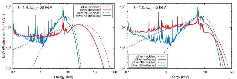
Figure 1: Comparison of the reflection calculations produced with the xillver code using the standard power-law illumination (red), and those produced with the new model xillverNS implementing a blackbody illumination spectrum (blue). The left panel shows the xillver case for $\Gamma$$=1.4$ and $E_{\mathrm{cut}}$$=50$ keV; while the right panel shows the extreme case of $\Gamma$$=1.0$ and $E_{\mathrm{cut}}$$=5$ keV. In both cases, the xillverNS is calculated for $kT_{\mathrm{bb}}$$=2$ keV. Other parameters common to all models are: $\log(\xi/$erg cm s${}^{-1})$$=3.1$, $A_{\mathrm{Fe}}$$=1$, $i=30$^∘, and $\log(n_{e}/$cm${}^{-3})$$=15$. The reflection fraction was set to $R_{\rm frac}=0$ when plotting the incident components, and to $R_{\rm frac}=-1$ when plotting the reflected components.

Finally, and in the same fashion of all our previous models, we produce a grid of synthetic spectra for a given set of input parameters, each covering a range of values appropriate for the astrophysical sources of interest. This model table is then self-consistently connected with our relativistic convolution model relconv (Dauser et al., 2010, 2013). The model takes into account the angular distribution of the solution provided by xillverNS and correctly predicts the integrated reflection off the disk by including all relativistic effects. This includes the distortion of the spectral features due to relativistic corrections such as boosting, gravitational redshift and Doppler effects. As described in García et al. (2014), this procedure is significantly different from simple convolution of the reflection spectrum, since a given line of sight will receive contributions from photons emitted at various angles due to light bending effects. This complete relativistic model is then referred to as relxillNS.

In the following, we describe the main parameters of the model, highlight the main differences with respect to reflection out of power-law illumination, and show detailed comparisons with previous calculations reported in the literature.

3 Results

3.1 X-ray Reflection in the Disk’s Frame

In this Section we describe the calculation of a new grid of reflection spectra in which the radiation field that illuminates the accretion disk takes the form of a blackbody spectrum. The resulting spectra are produced for a single slab at constant density, thus they represent reflection in the frame of the disk (i.e., ignoring relativistic effects). This new set of models are designed to be applicable for the case of irradiated accretion disks around neutron stars. The blackbody X-ray continuum is produced at the surface of the neutron star, or close to the surface from a boundary layer region, with typical temperatures in the $\sim 0.5-10$ keV range.

The shape of the illuminating radiation has a direct effect in controlling the ionization state and temperature profile of the atmosphere, and thus in determining the overall shape and spectral features of the reprocessed radiation. This effect is shown in Figure 1, where we compare the xillverNS calculations using a blackbody spectrum at a temperature of $kT_{\mathrm{bb}}$$=2$ keV, with the standard xillver spectra assuming a power-law illumination. The left panel shows a case representative of power-law reflection in black hole binaries, i.e., $\Gamma$$=1.4$, and $E_{\mathrm{cut}}$$=50$ keV. This spectrum shows a close resemblance to the xillverNS at energies below $\sim 2$ keV, but at higher energies the differences are evident. The power-law illumination has a larger number of photons at high energies, which contributes to a more pronounced Compton hump. Even when the parameters of the power-law are set to their extreme values in order to produce a spectrum closer to the blackbody in xillverNS, i.e., $\Gamma$$=1$ and $E_{\mathrm{cut}}$$=5$ keV (right panel, Figure 1), the differences in the resulting reflected spectra are large enough such that they will likely affect the spectral fitting to observational data.

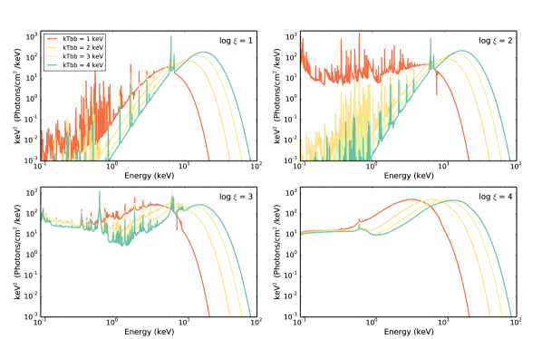
Figure 2: Effects of changing the temperature and overall flux of the illuminating radiation in the reflection spectra computed with the new xillverNS code. Each panel shows the reflected spectra for an increasing temperature $kT_{\mathrm{bb}}$ of the blackbody illumination at a given ionization parameter $\log(\xi/$erg cm s${}^{-1})$, as indicated. Other parameters common to all the models shown are: $A_{\mathrm{Fe}}$$=1$, $i=30$^∘, $\log(n_{e}/$cm${}^{-3})$$=15$, and $R_{\rm frac}=-1$ (i.e., only the reflection without the continuum spectrum is shown).

Given the relevance of the illuminating radiation in shaping the reprocessed spectrum, we have produced a full grid of reflection spectra using exclusively a blackbody at a given temperature $kT_{\mathrm{bb}}$. As in our previous models (García & Kallman, 2010; García et al., 2011, 2013), xillverNS assumes an illuminating spectrum incident at 45^∘ on the surface of a plane-parallel slab with constant density $n_{e}$. The slab has a total optical depth of 10, with no illumination from the bottom. The abundance of all astrophysically relevant elements is set to their Solar values based on the Grevesse & Sauval (1998) standard, with iron set at different values $A_{\mathrm{Fe}}$. The net incident flux (integrated in the $0.1-10^{3}$ keV range), is set to match a desired ionization parameter $\xi=4\pi F_{\mathrm{x}}/n_{e}^{2}$, for a given blackbody temperature $kT_{\mathrm{bb}}$ and density $n_{e}$. The complete set of parameters and the values used to produce the final grid of models is listed in Table 1.

Table 1: List of Parameters for the xillverNS Model

Parameter	Symbol (Units)	Range
Blackbody Temperature	$kT_{\mathrm{bb}}$ (keV)	$[0.5,10]$
Ionization Parameter	$\log(\xi/$erg cm s${}^{-1})$	$[1,4]$
Electron Number Density	$\log(n_{e}/$cm${}^{-3})$	$[15,19]$
Iron Abundance	$A_{\mathrm{Fe}}$ (Solar)	$[0.5,10]$

Figures 2, 3, and 4 show examples of the resulting calculations of the reflected spectra with xillverNS  for several combinations of model parameters. The overall behavior of these models is similar to any of the previous incarnations of the xillver calculations: the continuum of the reflected spectrum follows the general shape of the incident radiation (a blackbody in this case), with strong departures caused by a combination of photoelectric absorption, fluorescent emission, and absorption edges from the different ions in material; as well as the redistribution of photons due to Compton scattering.

Specifically, Figure 2 shows the effects of varying the illuminating radiation field by either changing the net incident flux (parameterized via $\xi$), or the temperature of the blackbody emission ($kT_{\mathrm{bb}}$). As expected, increasing the net flux results in a more ionized slab, which reduces the amount of spectral features. However, for a given value of $\xi$, increasing the temperature of the blackbody changes the bulk energy of the incident photons, producing strong changes in the spectrum. Models with higher $kT_{\mathrm{bb}}$ have more photons in the Fe K band, making the line emission more efficient, and producing a more noticeable Fe K-edge. Interestingly, for $\log(\xi/$erg cm s${}^{-1})$$\gtrsim 2$, the reflected continuum at low energies ($\lesssim 1$ keV) becomes much more prominent (and flatter) than the incident blackbody, due to the bremsstrahlung (free-free) emissivity.

Figure 3: Effects of changing the gas electron density for different illuminating fluxes in the reflection spectra computed with the new xillverNS code. Each panel shows the reflected spectra for increasing density $\log(n_{e}/$cm${}^{-3})$  at a given ionization parameter $\log(\xi/$erg cm s${}^{-1})$, as indicated. Other parameters common to all the models shown are: $A_{\mathrm{Fe}}$$=5$, $i=30$^∘, $kT_{\mathrm{bb}}$$=2$ keV, and $R_{\rm frac}=-1$ (i.e., only the reflection without the continuum spectrum is shown).

The effect of the increased bremsstrahlung emissivity due to an increment in the gas density is clearly depicted in Figure 3. Each panel show the comparison of the spectra reflected out slabs with different densities, but produced with the same illumination spectra. The higher the density, the more the flux in the reflected continuum at soft energies (see in particular the case for $\log(\xi/$erg cm s${}^{-1})$$=2$). This behavior resembles closely the reflection produced with a power-law illumination, as described in García et al. (2016). At higher densities the free-free heating is enhanced, raising the temperature of the atmosphere. This increases the amount of broadening in the spectral features through Compton scattering. The increased density and temperature may also increase the ionization of some species, which is likely the reason why the Fe K-edge appears less pronounced (e.g., see $\log(\xi/$erg cm s${}^{-1})$$=1$). At high ionization (e.g., $\log(\xi/$erg cm s${}^{-1})$$=3$) the changes in the soft flux are less severe, and in fact, at even higher ionization the effect is inverted. In the case of $\log(\xi/$erg cm s${}^{-1})$$=4$, the higher density models have the lower flux at $\sim 0.1$ keV. This is because the peak of the bremsstrahlung emissivity keeps shifting to higher energies, likely blending with the incident radiation field.

Finally, the effects of varying the iron abundance are exemplified in Figure 4. As in any of our previous xillver calculations, the iron abundance has a very predictable effect in the spectrum: any of the spectral profiles associated with iron, both in emission and absorption, are enhanced linearly with the increase of $A_{\mathrm{Fe}}$. In particular, the Fe K emission complex at $\sim 6.4-6.9$ keV becomes more intense with increased abundance, as well as the Fe K-edge ($\sim 7-9$ keV) becomes more prominent. This is also observed at lower energies, where other Fe transitions occur. A good example is the Fe L-shell emission complex near 1 keV. In the case of $\log(\xi/$erg cm s${}^{-1})$$=3$, the reflected flux at those energies increases by almost 2 orders of magnitude, when comparing the models with $A_{\mathrm{Fe}}$$=0.5$ and $A_{\mathrm{Fe}}$$=10$.

A closer inspection of Figure 4 shows an interesting aspect of these models. At soft energies (below $\sim 1$ keV), the effects of increasing the iron abundance seem to invert as the ionization parameter increases. At low $\xi$, larger iron abundance increases the photoelectric opacity causing a drop in the continuum. But at these energies the opacity is mostly dominated by low-$Z$ ions. However, more iron means that hard X-ray photons are absorbed more efficiently and at a much lower depth, which makes the overall ionization of the slab lower. Thus, at low ionization, the larger the abundance the more neutral the gas appears for the same incident radiation field. At high values of $\xi$ the situation changes, because most of the ions are either highly ionized or completely stripped. Thus, increasing the Fe abundance mostly contributes to increasing the gas temperature through photoionization heating, which increases the overall ionization state of the gas. In this regime, models with high iron abundance have the strongest flux at soft energies.

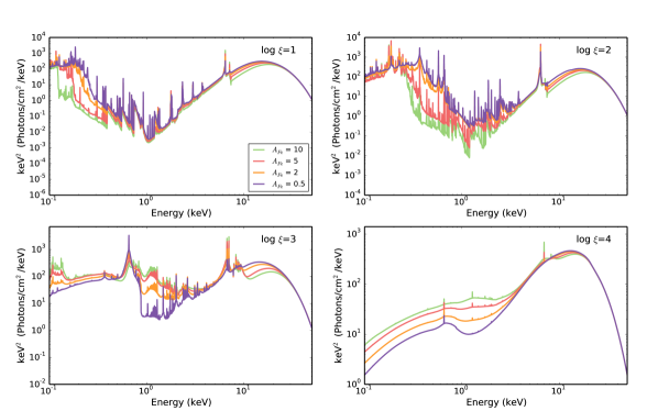
Figure 4: Effects of changing the content of iron for different illuminating fluxes in the reflection spectra computed with the new xillverNS code. Each panel shows the reflected spectra for iron abundance $A_{\mathrm{Fe}}$ (in Solar units), at a given ionization parameter $\log(\xi/$erg cm s${}^{-1})$, as indicated. Other parameters common to all the models shown are: $\log(n_{e}/$cm${}^{-3})$$=19$, $i=30$^∘, $kT_{\mathrm{bb}}$$=4$ keV, and $R_{\rm frac}=-1$ (i.e., only the reflection without the continuum spectrum is shown).

3.2 Relativistic Reflection

Similarly to the case of accretion disks around black holes, when the reflection of X-rays occurs in the regions of the accretion disk closer to the neutron star, reprocessed photons are affected by light-bending and energy shifts on their way to the observer. Doppler boosting and gravitational shifts take place causing a distortion of the spectrum, mainly affecting sharp atomic features. The magnitude of the spectral blurring increases close to the compact object. Thus, modeling in detail the spectral shapes provides estimates on the properties of the accretion disk, including its inner boundary. Under certain assumptions the inner radius of the disk can then be associated with the radius of the neutron star, or at the very least it provides a reasonable upper limit (Cackett et al., 2008).

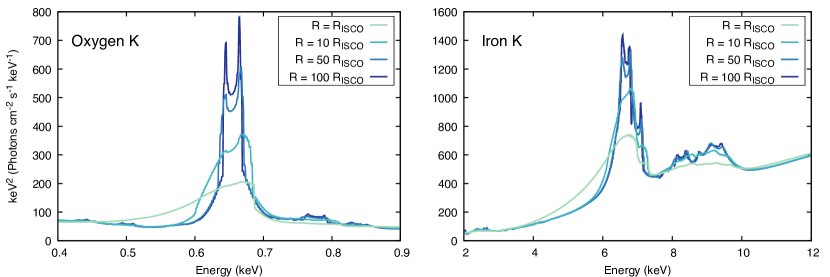
Figure 5: Reflection spectra produced with relxillNS for different values of disk truncation, as indicated. Left and right panels show the emission due to oxygen and iron K fluorescence, respectively. Other model parameters are: $q_{1}=q_{2}=3$, $a=0$, $i=30$^∘, $R_{\mathrm{out}}=10^{3}R_{g}$, $kT_{\mathrm{bb}}$$=4$ keV, $\log(\xi/$erg cm s${}^{-1})$$=3.1$, $A_{\mathrm{Fe}}$$=5$, $\log(n_{e}/$cm${}^{-3})$$=15$, and $R_{\mathrm{frac}}=1$ (i.e., including both reflection and continuum components).

Given the importance of properly modeling the relativistic effects in the reflected component, the reflection models discussed in the previous section (xillverNS) have been included in our suite of relativistic reflection models relxill (Dauser et al., 2014; García et al., 2014). This new flavor of our models, called relxillNS, calculates the total spectrum reprocessed in an accretion disk illuminated by a blackbody radiation field, by integrating the individual angle-dependent xillverNS reflection spectra emitted by different annuli and self-consistently including the relativistic effects. We note that all relativistic effects are computed using the Kerr metric, which correctly describes the space-time near for black holes and non rotating neutron stars. However, it is important to point out that deviations can occur from an induced quadrupole moment as the neutron star becomes oblate in structure as rotation rate increases. The Kerr metric is a good approximation for the space-time near a neutron star at low spin values, with a quadrupole-induced deviation of at most $10$% from the Kerr metric at $a=0.3$ (Sibgatullin & Sunyaev, 1998). The discrepancy becomes larger as break-up of the neutron star is approached ($\sim 25\%$, Sibgatullin & Sunyaev, 1998), but most neutron stars in LMXBs are expected to have a spin of $a_{*}\leq 0.3$ (Galloway et al., 2008; Miller et al., 2011).

As in previous models, the emissivity profile of the disk is assumed to follow a broken power-law profile with inner and outer emissivity indices, and breaking radius, taken as fit parameters. This is a parameterization of the illumination pattern rather than a physical model, given the uncertainty on the exact geometry of the primary source of photons. Meanwhile, Wilkins (2018) studied the illumination of disks around neutron stars using a fully relativistic ray tracing approach, producing theoretical emissivity profiles for illumination due to hotspots, bands of emission, and emission by the entirety of the spherical star surface. In all these cases, the emissivity is well described by a single power-law with the canonical index slightly steeper than the canonical value of $-3$.

Table 2: List of Parameters for the relxillNS Model

Parameter	Symbol (Units)	Range
Inner Emissivity Index	$q_{1}$	$[-10,10]$
Outer Emissivity Index	$q_{2}$	$[-10,10]$
Break Radius	$R_{\mathrm{Br}}$ ($R_{g}$)	$[1-1000]$
Spin Parameter	$a_{*}$ ($cJ/GM^{2}$)	$[-0.998,0.998]$
Inclination	$i$ (degrees)	$[3,87]$
Inner Disk Radius	$R_{\mathrm{in}}$ ($R_{\mathrm{ISCO}}$)	$[1,1000]$
Outer Disk Radius	$R_{\mathrm{out}}$ ($R_{g}$)	$[1,1000]$
Blackbody Temperature	$kT_{\mathrm{bb}}$ (keV)	$[0.5,10]$
Ionization Parameter	$\log(\xi/$erg cm s${}^{-1})$	$[1,4]$
Electron Number Density	$\log(n_{e}/$cm${}^{-3})$	$[15,19]$
Iron Abundance	$A_{\mathrm{Fe}}$ (Solar)	$[0.5,10]$
Reflection Fractiona	$R_{\mathrm{frac}}$	$[0,10]$

In addition to the parameters describing the reflection spectra (see Table 1), other model parameters include the dimensionless spin parameter, inclination, inner and outer radius of the disk, and the reflection fraction. The latter controls the proportion of the blackbody continuum to the reflection component. Given that the exact origin of the blackbody emission is unknown, and its geometry is not specified, we parametrize the emissivity profile as a power-law. Thus, a self-consistent calculation of the reflection fraction is not possible with this model. For the same reasons, it is not possible to derive a physical interpretation of the fitted values. However, the reflection fraction does provides some clues on the possible geometry of the region responsible for the primary emission, as relativistic effects strongly affect its value. For example, reflection dominated spectra are only likely for compact emitting regions, for which relativistic beaming reduces the flux of the primary component and enhances the reflection fraction.

The full list of parameters with their allowed ranges is summarized in Table 2. Figure 5 shows a series of reflected spectra produced with relxillNS for different values of the inner radius (i.e., for different degrees of disk truncation), looking in particular at the emission due to oxygen and iron K transitions. Traditionally, reflection spectroscopy studies had focused on the Fe K emission given its prominence in the X-ray spectra. However, in cases where the continuum is much softer than a power-law, such as is the case of the blackbody illumination in relxillNS, lines from lower-$Z$ elements can also become important probes of relativistic effects. The oxygen K emission lines are a good example of an alternative atomic feature that can be used for the estimation of the disk radius and other model parameters.

3.3 Comparisons with other reflection models

In this Section we present a detailed discussion of the performance of the xillverNS and relxillNS models, and compare them with other reflection models previously published.

3.3.1 Fits to the neutron star 4U 1705$-$44

As a reference source we have chosen the low mass X-ray binary neutron star system 4U 1705$-$44, which is a well studied bursting source that displays strong signatures of disk reflection in the X-ray spectrum. Previous XMM-Newton observations taken in the hard and soft states have been analyzed by di Salvo et al. (2009); D’Aì et al. (2010), and Egron et al. (2013). All these works reported the presence of iron K-shell emission lines, as well as several other emission features at softer energies associated with lower-$Z$ elements like argon and calcium. As discussed in Egron et al. (2013), Ar and Ca lines were not included in earlier reflection codes, until the production of the xillver models.

Although it is clear that the largest discrepancies between different generations of reflection models are most significant at softer energies, where the largest amount of spectral lines are observed, the reflection models featured in this paper (xillverNS, relxillNS) are generally intended for observations from sources in soft states, where the continuum is dominated by thermal emission (both from the disk and from the neutron star), which it is expected to overcome the reflection component at soft energies. In some systems, however, the accretion disk does not extend down to the surface of the neutron star, but it is rather truncated at a few gravitational radii, likely due to the presence of a boundary layer. This causes a fainter disk emission, allowing for the soft energy features of the reflection spectrum to be observed. Thus, accurate reflection models with updated atomic data for all relevant species are necessary to constraint the physical parameters that describe the accretion flow around neutron stars.

In any case, detailed comparisons of spectral features at energies below the NuSTAR bandpass require analysis of data from other observatories, which are prone to vetting instrumental effects such as photon pile-up (in the case of XMM-Newton; however, see Egron et al., 2013), or uncertain calibration (in the case of NICER). This would require a much more careful and complicated analysis, far beyond the scope of the present paper.

We thus restrict our analysis and comparison of all the models to the same observational dataset: a 29 ks spectrum in the $3-30$ keV X-ray band observed with both Focal Plane Modules onboard of NuSTAR. This observation was previously analyzed by Ludlam et al. (2017c) with the BBrefl and reflionx_BB models. The data was reduced using the standard mission procedures as described in Ludlam et al. (2017c). In general, the models applied to the NuSTAR observations of 4U 1705$-$44 have the same structure: a multi-temperature disk emission spectrum modeled with diskbb (Mitsuda et al., 1984; Makishima et al., 1986), plus a single temperature blackbody component (likely originating from the surface or boundary region of the neutron star), and its corresponding reflection spectrum. Galactic absorption is modeled with the TBabs model assuming Wilms et al. (2000) abundances and Verner et al. (1996) cross sections. Relativistic effects that distort the reflected radiation produced close to the neutron star are included via the convolution model relconv (Dauser et al., 2010, 2013). Thus, in xspec notation the models are written as:

• TBabs*(diskBB+relconv$\otimes$BBrefl)

• TBabs*(diskBB+relxillNS)

• TBabs*(diskBB+BBody+relconv$\otimes$reflionx_BB)

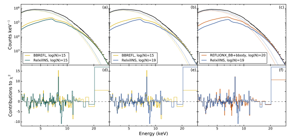
Figure 6: Spectral fits to the NuSTAR data of the neutron star 4U 1705$-$44, using three different reflection models: BBrefl, relxillNS and reflionx_BB. Each column shows a comparison of the fits using relxillNS and BBrefl (left and middle columns), and reflionx_BB (right column). The top row shows the model components (blackbody continuum, dotted) and reflection spectrum (solid color lines), and the the total relxillNS model applied to the observational data (black solid line and data points, respectively). The panels in the bottom row show the contributions to $\chi^{2}$ from each fit.

Here, both BBrefl (Ballantyne, 2004) and reflionx_BB are based on the same parent code reflionx (Ross & Fabian, 2005), with the difference they both assume a blackbody illumination spectrum, rather than the standard power-law. Moreover, BBrefl assumes local thermo-dynamical equilibrium (LTE) throughout the slab, while reflionx_BB produces a non-LTE calculation that predicts the local flux at each depth, which accounts for differences in the line profiles. Reflionx_BB was constructed as a simple, generally applicable model for reflection in neutron stars. It uses the standard reflionx code, without additional physics, but replacing the power-law illumination with a black body spectrum and increasing the density from $10^{15}$ cm^-3 to $10^{20}$ cm^-3. It covers a wide range in ionization ($10-10^{4}$ erg cm s^-1), iron abundance ($0.1-10$ Solar) and black body temperature ($0.1-10$ keV). Reflionx_BB also has a broader range of elements, charge states, and ionization than BBRefl. We have chosen a version of BBrefl with iron abundance fixed to twice the Solar value, and gas density of $\log(n_{e}/$cm${}^{-3})$$=15$. Note that BBrefl provides the blackbody continuum, and thus this component does not need to be explicitly included. The same applies to relxillNS, which also self-consistently includes all relativistic blurring effects, and thus the relconv convolution model is also not required.

Table 3: Comparison of the best-fit parameters to NuSTAR data of 4U 1705$-$44 using different reflection models

Component	Parameter	Model 1	Model 2		Model 3
TBabs	$N_{\mathrm{H}}(10^{22}$ cm${}^{-2})$	$0.7$	$0.7$	$0.7$	$0.7$
diskbb	$T_{\mathrm{in}}$ (keV)	$2.01^{+0.05}_{-0.04}$	$2.14^{+0.06}_{-0.06}$	$2.14^{+0.03}_{-0.04}$	$1.95^{+0.02}_{-0.04}$
diskbb	$N_{\mathrm{d}}$	$11.4^{+0.6}_{-0.8}$	$9.5^{+0.8}_{-0.7}$	$9.7^{+0.5}_{-0.4}$	$12.5^{+0.9}_{-0.3}$
BBody	$kT$ (keV)	$\cdots$	$\cdots$	$\cdots$	$2.53^{+0.02}_{-0.03}$
BBody	$N_{\mathrm{BB}}$ $(10^{-2})$	$\cdots$	$\cdots$	$\cdots$	$1.21^{+0.06}_{-0.10}$
relconv	$q$	$3.45^{+0.39}_{-0.40}$	$\cdots$	$\cdots$	$3.29^{+0.46}_{-0.84}$
relconv	$a_{*}$ ($cJ/GM^{2}$)	$0.0$	$\cdots$	$\cdots$	$0.0$
relconv	$i$ (∘)	$25.5^{+0.9}_{-2.6}$	$\cdots$	$\cdots$	$24.7^{+1.2}_{-11.5}$
relconv	$R_{\mathrm{in}}$ (ISCO)	$1.53^{+0.15}_{-0.19}$	$\cdots$	$\cdots$	$1.49^{+0.49}_{-0.16}$
relconv	$R_{\mathrm{out}}$ ($R_{g}=GM/c^{2}$)	$990$	$\cdots$	$\cdots$	$990$
BBrefl	$\log(n_{e}/$cm${}^{-3})$	$15$	$\cdots$	$\cdots$	$\cdots$
BBrefl	$\log(\xi/$erg cm s${}^{-1})$	$2.71^{+0.16}_{-0.09}$	$\cdots$	$\cdots$	$\cdots$
BBrefl	$kT$ (keV)	$2.67^{+0.05}_{-0.03}$	$\cdots$	$\cdots$	$\cdots$
BBrefl	$A_{\mathrm{Fe}}$ (Solar†)	$2$	$\cdots$	$\cdots$	$\cdots$
BBrefl	$f_{\mathrm{refl}}$	$0.76^{+0.16}_{-0.07}$	$\cdots$	$\cdots$	$\cdots$
BBrefl	$N_{\mathrm{BBR}}$ $(10^{-26})$	$2.2^{+0.4}_{-0.8}$	$\cdots$	$\cdots$	$\cdots$
reflionx_BB	$\log(n_{e}/$cm${}^{-3})$	$\cdots$	$\cdots$	$\cdots$	$20$
reflionx_BB	$\xi$ (erg cm s-1)	$\cdots$	$\cdots$	$\cdots$	$407\pm 218$
reflionx_BB	$A_{\mathrm{Fe}}$ (Solar†)	$\cdots$	$\cdots$	$\cdots$	$2.7^{+1.4}_{-1.7}$
reflionx_BB	$N_{\mathrm{RX}}$	$\cdots$	$\cdots$	$\cdots$	$0.57\pm 0.14$
relxillNS	$q$	$\cdots$	$3.7^{+0.7}_{-0.3}$	$3.9^{+0.8}_{-0.4}$	$\cdots$
relxillNS	$a_{*}$ ($cJ/GM^{2}$)	$\cdots$	$0$	$0$	$\cdots$
relxillNS	$i$ (∘)	$\cdots$	$30.5^{+1.0}_{-1.1}$	$30.9^{+1.0}_{-1.0}$	$\cdots$
relxillNS	$R_{\mathrm{in}}$ (ISCO)	$\cdots$	$1.74^{+0.18}_{-0.22}$	$1.64^{+0.18}_{-0.22}$	$\cdots$
relxillNS	$R_{\mathrm{out}}$ ($R_{g}=GM/c^{2}$)	$\cdots$	$990$	$990$	$\cdots$
relxillNS	$kT_{\mathrm{BB}}$ (keV)	$\cdots$	$2.80^{+0.13}_{-0.08}$	$2.90^{+0.09}_{-0.07}$	$\cdots$
relxillNS	$\log(n_{e}/$cm${}^{-3})$	$\cdots$	$15$	$19$	$\cdots$
relxillNS	$\log(\xi/$erg cm s${}^{-1})$	$\cdots$	$2.64^{+0.07}_{-0.04}$	$2.56^{+0.02}_{-0.01}$	$\cdots$
relxillNS	$A_{\mathrm{Fe}}$ (Solar†)	$\cdots$	$2.63$	$2.63$	$\cdots$
relxillNS	$R_{f}$	$\cdots$	$0.9^{+0.7}_{-0.3}$	$1.3^{+0.6}_{-0.4}$	$\cdots$
relxillNS	$N_{\mathrm{XNS}}$ ($10^{-4}$)	$\cdots$	$4.6^{+2.0}_{-1.9}$	$3.3^{+1.1}_{-1.0}$	$\cdots$
	$\chi^{2}$	$797.59$	$801.50$	$789.91$	$809.16$
	$\nu$	$665$	$665$	$665$	$664$
	$\chi_{\nu}^{2}$	$1.20$	$1.21$	$1.19$	$1.22$

The best-fit parameters and statistics for the goodness of the fits are summarized in Table 3. In all the cases, we fixed the hydrogen column density to the Kalberla et al. (2005) value, and the spin parameter to zero. The disk density in relxillNS (Model 2) was also fixed to match as close as possible the values assumed in BBrefl ($10^{15}$ cm^-3) and reflionx_BB ($10^{20}$ cm^-3). Thus, for Model 2 we present results fixing the density to $10^{15}$ and $10^{19}$ cm^-3 (the latter being the maximum value possible in the current version of our model). The results show that the density has a minor effect on the quality of the fits. The majority of the model parameters are consistent among these fits: importantly, the blackbody temperature, inner disk radius, and ionization parameter are all in agreement within their uncertainty levels. Iron abundance is in good agreement between Models 1 and 2, when the differences in the Solar value are considered (see caption in Table 3). The fits with relxillNS (Model 2) yield disk inclinations a few degrees higher than the other two models, likely due to differences in the atomic data implemented by each code, which can affect the details of the Fe K emission profile. In general, the three models provide fits of comparable quality, with only a marginal preference of relxillNS (Model 2) using the highest density value ($\log(n_{e}/$cm${}^{-3})$$=19$), with a $\chi^{2}$ of 790 compared to 798 of BBrefl (both for 665 degrees of freedom, d.o.f.), and 809 for reflionx_BB for 664 d.o.f.

A comparison of the performance of the different fits in reproducing the NuSTAR data in the $3-30$ keV region is shown in Figure 6, where we include the model components (incident blackbody and reflection spectra), the total model with the data, and the residuals of each fit. We compare the relxillNS fit (Model 2) with low and high density against the BBrefl fit (Model 1), and against the reflionx_BB fit (Model 3) for the high density case. In all cases the strongest residuals are seen at high energies, above $\sim 20$ keV, where the source counts start to get dominated by the background. An additional narrow emission feature is observed at $\sim 8$ keV, as well as some absorption at $\sim 8.5$ keV, whose origin is unclear. However, we emphasize that the analysis presented here is intended for comparative purposes only, and thus a more detailed examination of the physics of this system is left for future publications. The residuals show otherwise a relatively similar fit by all the models, as also demonstrated by the fit statistics.

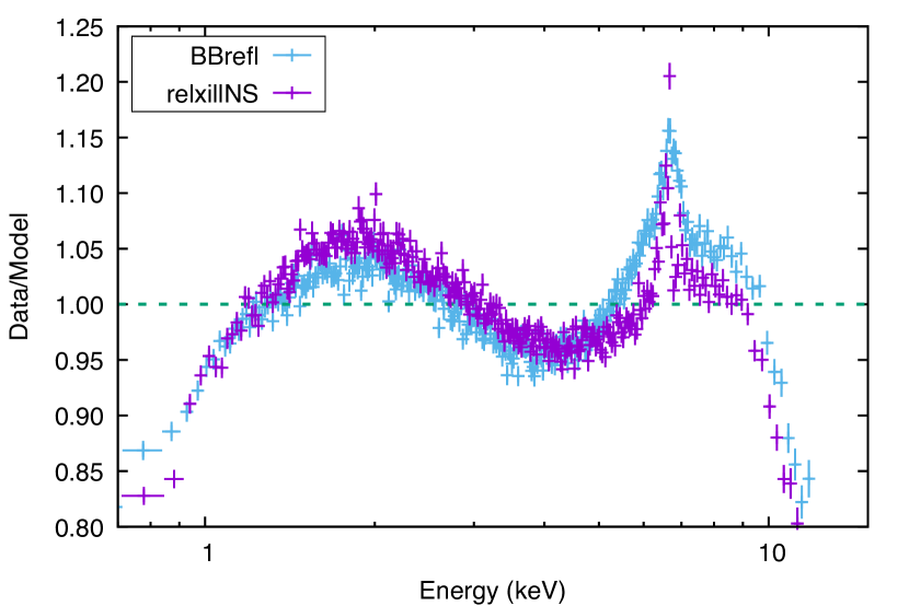
Figure 7: Ratio plot of simulated XRISM-Resolve observations to an absorbed blackbody plus power-law model. The simulations were produced using the best-fit parameters for Model 1 (based on BBrefl) and Model 2 (based on relxillNS). In both cases we use the Resolve response matrix for a 5 eV spectral resolution at 6 keV, and a exposure time of 20 ks.

3.3.2 XRISM Simulations

Although the fits discussed in the previous Section yielded results with very similar statistical quality, the different models implemented are not identical. It is thus expected that the new generation of X-ray observatories with improved effective area and spectral resolution will provide data with sufficient signal to distinguish between these models. To demonstrate this, we have carried out simulations of observational data using the instrumental response for the Resolve instrument onboard of the X-Ray Imaging and Spectroscopy mission (XRISM) (Tashiro et al., 2018). Resolve is a soft X-ray micro-calorimeter spectrometer, which provides non-dispersive $5-8$ eV energy resolution in the $0.3-12$ keV bandpass.

Specifically for these simulations, we have used the most optimistic RMFs for 5 eV resolution together with the ARF files for the case of gate-valve open (i.e., no filter). The simulations were produced with the fakeit routine in xspec, based on the best-fits produced with Model 1 (which is based on BBrefl) and Model 2 (based on relxillNS), for the NuSTAR data of 4U 1705$-$44 shown in the previous Section. The flux predicted by this fit is close to 100 mCrab in the $2-10$ keV band, and we assumed a 20 ks exposure time for each simulation.

Figure 7 shows the two XRISM-Resolve simulations as a ratio plot of the data to a model for the continuum, based on an absorbed blackbody plus power-law model. We note that the power-law is included to provide a continuum that better resembles the observations and improve clarity in the ratio plot. The superior energy resolution of the micro-calorimeter makes evident the differences between these two models, particularly in the shape of Fe K emission, as well as the overall shape of the continuum at softer energies. Interestingly, relxillNS predicts a narrower Fe K profile than BBrefl. Given that the two models were evaluated for similar parameters (e.g., ionization, spin, inner radius, inclination), the difference in the width of the emission cannot be due to a different relativistic smearing, but rather to the intrinsic shape of the reflection spectrum in the local frame. When relativistic effects are excluded, the most significant source of line broadening is due to Comptonization of reflected photons in the hot layers of the disk’s atmosphere. Photons are shifted to higher or lower energies due to electron scattering, depending on the optical depth and temperature of the material. In fact, for high enough temperatures ($T\sim 10^{7}-10^{8}$ K), the Compton kernel is dominated by the contribution of the kinetic energy of the electrons, causing a rather symmetric broadening of spectral features (García et al., 2020). The differences observed between relxillNS and BBrefl suggests a dissimilar solution for the state of the gas between the two models. Our simulations show that such discrepancies can only be distinguished with the superior energy resolution of future instruments. Conversely, this simple comparison demonstrates the importance of accurate models for the upcoming generation of X-ray instruments.

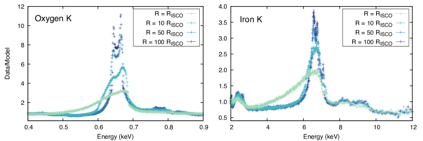
Figure 8: Ratio plot of Athena X-IFU simulations to an absorbed blackbody plus power-law model. The simulations were generated with relxillNS for different values of disk truncation, using the same parameters of the models in Figure 5. In all the cases, the exposure time is 10 ks for a flux source of 10 mCrab.

3.3.3 Athena Simulations

In order to further emphasize the diagnostic power of our new reflection models in combination with the enhanced instrumental capabilities of planned facilities, we have also carried out simulations for the flagship mission Athena (Advanced Telescope for High Energy Astrophysics; Nandra et al., 2013), currently under development and planned to be operational in the mid 2030’s. The X-ray Integral Field Unit (X-IFU) is Athena’s micro-calorimeter spectrometer, which is expected to deliver data with an unprecedented energy resolution of 2.5 eV or better up to 7 keV (Barret et al., 2018).

In this case we carried out simulations based on the relxillNS models presented in Section 3.2 (shown in Figure 5), i.e., $q_{1}=q_{2}=3$, $a=0$, $i=30$^∘, $R_{\mathrm{out}}=10^{3}R_{g}$, $kT_{\mathrm{bb}}$$=4$ keV, $\log(\xi/$erg cm s${}^{-1})$$=3.1$, $A_{\mathrm{Fe}}$$=5$, $\log(n_{e}/$cm${}^{-3})$$=15$, and $R_{\mathrm{frac}}=1$ (including both reflection and continuum components). The four different cases shown correspond to models with disk inner radius set at $1,10,50$, and $100R_{\mathrm{ISCO}}$, as indicated. For all these cases Galactic absorption is included via the TBabs model assuming a low H column density of $N_{H}=10^{20}$ cm^-2, and a source flux of 10 mCrab. Sources with fluxes of $\sim 100$ mCrab or more will require a defocussed mode (which degrades the energy resolution), in order to prevent photon pile-up. However, owing to the significantly larger effective area of Athena, observations of moderately bright source (10 mCrab) with a exposure of 10 ks will provide sufficient signal-to-noise to resolve most of the structure of relativistically broadened atomic lines.

The X-IFU simulations are shown in Figure 8, which displays the same energy ranges depicted in Figure 5 for the O and Fe K-shell transitions. These simulations clearly show that with relatively short observations precise constraints on important parameters like the disk inner radius will be easily achievable. The details of the line emission are almost fully resolved, particularly in the case of the O K emission, where the double horn of the line profile is clearly resolved at even large truncation radii. However, we note that the conditions for the present simulations are overly optimistic: we have chosen to simulate the case of a source with very low Galactic absorption with no disk emission (only the blackbody continuum and its corresponding reflection components are included), in order to emphasize the strength of the O K emission. In reality, most of the sources for which relxillNS was designed are expected to show a strong disk component which will likely outshine the reflection emission at soft energies, making the detection of oxygen lines challenging. Nevertheless, this example demonstrates the potential capabilities of future instruments in resolving the detailed structure of the spectral profiles.

3.3.4 Comparison with convolution models

Another model used for the analysis of neutron star X-ray spectra is xilconv, which is an updated version of the rfxconv model (Kolehmainen et al., 2011), as first described in Done & Gierliński (2006). The only difference between these two models is that rfxconv uses the reflection tables produced with the reflionx code, while xilconv uses those from xillver. These models act as a convolution kernel upon any spectral component, allowing the user to input any desired continuum spectrum. The model then determines the average power-law index in the $2-10$ keV region, and selects the corresponding reflection spectra from the precomputed table. The main caveat of this procedure is the lack of self-consistency between the input spectrum and the reflection, as the latter is always chosen from the standard xillver library computed with the illumination in form of a power-law, regardless of what input spectrum is selected. This model is thus prone to spurious results while fitting observational data. This is demonstrated in Figure 9, where we compare the xillverNS spectra with those predicted by a xilconv$\otimes$bbody model with the same input parameters. We found that for low ionization parameters the two models compare reasonably well. However, at higher ionization the discrepancy is striking: the overall shape of the reflection spectrum is dramatically different at all energies, with xilconv consistently under-predicting the flux at soft energies, and over-predicting the Fe K emission. We thus advise against the use of these models, particularly in cases where the input spectrum is different from the standard power-law shape.

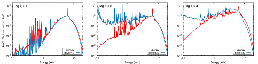
Figure 9: Comparison of xillverNS spectra with those predicted by the xilconv$\otimes$bbody model, for three different values of the ionization parameter $\log(\xi/$erg cm s${}^{-1})$, as indicated. For all these cases the other model parameters are: $kT_{\mathrm{bb}}$$=1$ keV, $A_{\mathrm{Fe}}$=1, $\log(n_{e}/$cm${}^{-3})$$=15$, $i=60$ ^∘, and $R_{\rm frac}=-1$. The xillverNS spectra were re-normalized such that the input blackbody spectrum in the two models are the same when $R_{\rm frac}=0$.

4 Discussion & Conclusions

We have presented new X-ray reflection models for geometrically-thin, optically-thick accretion disks around compact objects. The illumination spectrum is assumed to be a blackbody emission at a given temperature, which after being reprocessed by the disk, produces a reflection spectrum with characteristic signatures of great diagnostic potential. The new reflection models featured here, xillverNS, and its relativistic counterpart relxillNS, are primarily intended for the interpretation of the X-ray spectrum observed from accretion disks around neutron stars, which are now commonly observed with current X-ray satellites. The superior capabilities of the XMM-Newton, NICER and NuSTAR observatories have opened new venues to study these systems, and thus accurate X-ray reflection models are crucial for the interpretation of new observational data. Similar reflection models have been produced in the past with outdated codes and atomic databases (e.g. Ballantyne, 2004; Ross & Fabian, 2007). Here, we provide a major update by implementing angle-resolved radiative transfer calculations which make use of the most up-to-date collection of atomic parameters for inner-shell transitions.

A simple test case to the NuSTAR data of 4U 1705$-$44 shows a satisfactory performance of the new relxillNS in describing the observational data. Comparisons of fits with earlier models like BBrefl and reflionx_BB show very good consistency between the models. Although the newer atomic database included in relxillNS is expected to have a more significant impact at softer energies, we defer such a detailed analysis for future publications. Meanwhile, simulations of observations with new generation of X-ray observatories such as XRISM-Resolve and Athena X-IFU revealed the large diagnostic potential of these new models in describing the detailed structure of the reprocessed emission, which will be required to describe the high-resolution spectrum delivered by upcoming micro-calorimeter instruments.

Preliminary versions of the xillverNS and relxillNS models shown in this paper have already been implemented in several previous works. The model has been tested and used on a NICER observation of Serpens X-1 (Ludlam et al., 2018), a NuSTAR observation of GX 3+1 (Ludlam et al., 2019a), and a joint NICER and NuSTAR observation of 4U 1735$-$44 (Ludlam et al., 2020). These are all persistently accreting “atoll” sources (named after characteristic island-like patterns that are traced out in hardness-intensity and color-color diagrams; Hasinger & van der Klis, 1989).

In all spectral fits, the models have been able to successfully describe the data, providing evidence for relativistically smeared atomic lines. The density of the inner disk was inferred to be higher than the $10^{15}$ cm^-3 that used to be the standard value assumed in reflection models. The emissivity index is less than 4, which is consistent with expectations for a disk illuminated by a neutron star (Wilkins, 2018). The limits on inner disk radius constrained via relxillNS allowed for limits to be placed on the dipolar magnetospheric strengths of the neutron stars and presence of boundary layer regions in these systems. Serpens X-1, in particular, was a useful test since this source exhibited multiple broad emission features (i.e., Fe L and Fe K). Through employing the relxillNS model it became clear that the Fe L emission profile was more complex than a single line, but rather a blend of emission from lower-$Z$ elements, such as Mg iii-vii (see Figure 4 in Ludlam et al., 2018).

Unexpectedly, these models have also played a fundamental role in the detection of returning disk radiation. This is a general relativistic effect theoretically predicted by Cunningham (1976), in which thermal disk photons are returned to the other regions of the disk due to the strong gravitational bending. The first observational evidences for returning radiation was recently found in soft-state observations of several black hole binaries, such as XTE J1550$-$564 (Connors et al., 2020), 4U 1630$-$47 (Connors et al., 2021), EXO 1846-031 (Wang et al., 2021), and MAXI J0637$-$430 (Lazar et al., 2021). In all these works, the relxillNS model was implemented in the spectral fits as a proxy for reflection produced by returning disk radiation.

We note that the present setup of relxillNS is somewhat simplistic, as it only considers illumination with a single temperature thermal emitter. Future versions of these models will likely be expanded to also include non-thermal illumination (i.e., power-law) in combination with the blackbody emission, in order to closely resemble the X-ray continuum observed in several neutron star systems such as Serpens X-1 (Cackett et al., 2008), 4U 1728$-$34 (Sleator et al., 2016), Aquila X-1 (Ludlam et al., 2017b), XTE J1709$-$267 (Ludlam et al., 2017a), and 4U 1543$-$624 (Ludlam et al., 2019b), among several others. Modern observations have shown that the power-law continuum is best modelled with a thermal Comptonization model (Matranga et al., 2017), just like in the case of black hole binaries. We thus plan to implement the newest version of the thComp mode (Zdziarski et al., 2020) in upcoming version of relxillNS, in close similarity to the relxillCp family of models (note, however, that in relxillCp there is not thermal component in the illuminating spectrum).

Implementing a Comptonization continuum to fit neutron stars will also require the possibility for a variable photon seed temperature, that can be set well above the fixed value of $0.05$ keV in the current relxillCp models. This will be particularly important for sources in the soft state, where the disk temperature can reach the $0.5-1$ keV range. Such a model feature will also be useful to correctly reproduce sources in the intermediate state (especially atoll sources), which display an X-ray continuum departing from a simple blackbody spectrum.

A relatively weak and steep power-law in addition to the thermal components can also be observed during the soft states of Z and atoll sources, with photon indices larger than 2 and an overall flux of no more than $10\%$ of the total emission (see, Di Salvo et al., 2000; D’Amico et al., 2001; Piraino et al., 2007; Pintore et al., 2016). However, in these cases the contribution of the power-law component to the illuminating spectrum is weak and will no likely affect the reflection spectrum in a significant manner.

Another limitation of the models presented here is due to the fact that it uses the Kerr metric to describe the space-time near the compact object. Technically, this metric is correct for black holes, and sufficiently accurate for non rotating neutron stars, but it becomes increasingly inaccurate for larger spins. The exact metric near a neutron star depends on its mass and equation of state, which are largely unknown. We thus caution users to proceed with care when allowing non-zero spins while fitting data neutron star systems, and we generally recommend no to exceed spin values above $a_{*}=0.3$. Both the new reflection model flavor relxillNS, and its non-relativistic counterpart xillverNS, are publicly distributed to the community in our suite of models relxill, v-1.5.0.

References

- Arnaud (1996) Arnaud, K. A. 1996, in Astronomical Society of the Pacific Conference Series, Vol. 101, Astronomical Data Analysis Software and Systems V, ed. G. H. Jacoby & J. Barnes, 17
- Ballantyne (2004) Ballantyne, D. R. 2004, MNRAS, 351, 57, doi: 10.1111/j.1365-2966.2004.07767.x
- Barret et al. (2018) Barret, D., Lam Trong, T., den Herder, J.-W., et al. 2018, in Society of Photo-Optical Instrumentation Engineers (SPIE) Conference Series, Vol. 10699, Space Telescopes and Instrumentation 2018: Ultraviolet to Gamma Ray, ed. J.-W. A. den Herder, S. Nikzad, & K. Nakazawa, 106991G
- Bhattacharyya & Strohmayer (2007) Bhattacharyya, S., & Strohmayer, T. E. 2007, ApJ, 664, L103, doi: 10.1086/520844
- Cackett et al. (2009) Cackett, E. M., Altamirano, D., Patruno, A., et al. 2009, ApJ, 694, L21, doi: 10.1088/0004-637X/694/1/L21
- Cackett et al. (2012) Cackett, E. M., Miller, J. M., Reis, R. C., Fabian, A. C., & Barret, D. 2012, ApJ, 755, 27, doi: 10.1088/0004-637X/755/1/27
- Cackett et al. (2008) Cackett, E. M., Miller, J. M., Bhattacharyya, S., et al. 2008, ApJ, 674, 415, doi: 10.1086/524936
- Cackett et al. (2010) Cackett, E. M., Miller, J. M., Ballantyne, D. R., et al. 2010, ApJ, 720, 205, doi: 10.1088/0004-637X/720/1/205
- Chiang et al. (2016) Chiang, C.-Y., Cackett, E. M., Miller, J. M., et al. 2016, ApJ, 821, 105, doi: 10.3847/0004-637X/821/2/105
- Connors et al. (2021) Connors, R., García, J., Tomsick, J., et al. 2021, arXiv e-prints, arXiv:2101.06343. https://arxiv.org/abs/2101.06343
- Connors et al. (2020) Connors, R. M. T., García, J. A., Dauser, T., et al. 2020, ApJ, 892, 47, doi: 10.3847/1538-4357/ab7afc
- Cunningham (1976) Cunningham, C. 1976, ApJ, 208, 534, doi: 10.1086/154636
- D’Aì et al. (2010) D’Aì, A., di Salvo, T., Ballantyne, D., et al. 2010, A&A, 516, A36, doi: 10.1051/0004-6361/200913758
- D’Amico et al. (2001) D’Amico, F., Heindl, W. A., Rothschild, R. E., & Gruber, D. E. 2001, ApJ, 547, L147, doi: 10.1086/318902
- Dauser et al. (2014) Dauser, T., García, J., Parker, M., Fabian, A., & Wimls, J. 2014, Submitted to MNRAS, 430, 1694
- Dauser et al. (2016) Dauser, T., García, J., & Wilms, J. 2016, Astronomische Nachrichten, 337, 362, doi: 10.1002/asna.201612314
- Dauser et al. (2013) Dauser, T., Garcia, J., Wilms, J., et al. 2013, MNRAS, 430, 1694, doi: 10.1093/mnras/sts710
- Dauser et al. (2010) Dauser, T., Wilms, J., Reynolds, C. S., & Brenneman, L. W. 2010, MNRAS, 409, 1534, doi: 10.1111/j.1365-2966.2010.17393.x
- Degenaar et al. (2015) Degenaar, N., Miller, J. M., Chakrabarty, D., et al. 2015, MNRAS, 451, L85, doi: 10.1093/mnrasl/slv072
- Degenaar et al. (2016) Degenaar, N., Altamirano, D., Parker, M., et al. 2016, MNRAS, 461, 4049, doi: 10.1093/mnras/stw1593
- Di Salvo et al. (2000) Di Salvo, T., Stella, L., Robba, N. R., et al. 2000, ApJ, 544, L119, doi: 10.1086/317309
- di Salvo et al. (2009) di Salvo, T., D’Aí, A., Iaria, R., et al. 2009, MNRAS, 398, 2022, doi: 10.1111/j.1365-2966.2009.15240.x
- Done & Gierliński (2006) Done, C., & Gierliński, M. 2006, MNRAS, 367, 659, doi: 10.1111/j.1365-2966.2005.09968.x
- Egron et al. (2013) Egron, E., Di Salvo, T., Motta, S., et al. 2013, A&A, 550, A5, doi: 10.1051/0004-6361/201219675
- Fabian & Ross (2010) Fabian, A. C., & Ross, R. R. 2010, Space Sci. Rev., 157, 167, doi: 10.1007/s11214-010-9699-y
- Feautrier (1964) Feautrier, P. 1964, Comptes Rendus Academie des Sciences (serie non specifiee), 258, 3189
- Freeman et al. (2001) Freeman, P., Doe, S., & Siemiginowska, A. 2001, in Society of Photo-Optical Instrumentation Engineers (SPIE) Conference Series, Vol. 4477, Astronomical Data Analysis, ed. J.-L. Starck & F. D. Murtagh, 76–87
- Galloway et al. (2008) Galloway, D. K., Muno, M. P., Hartman, J. M., Psaltis, D., & Chakrabarty, D. 2008, ApJS, 179, 360, doi: 10.1086/592044
- García et al. (2013) García, J., Dauser, T., Reynolds, C. S., et al. 2013, ApJ, 768, 146, doi: 10.1088/0004-637X/768/2/146
- García & Kallman (2010) García, J., & Kallman, T. R. 2010, ApJ, 718, 695, doi: 10.1088/0004-637X/718/2/695
- García et al. (2011) García, J., Kallman, T. R., & Mushotzky, R. F. 2011, ApJ, 731, 131, doi: 10.1088/0004-637X/731/2/131
- García et al. (2014) García, J., Dauser, T., Lohfink, A., et al. 2014, ApJ, 782, 76, doi: 10.1088/0004-637X/782/2/76
- García et al. (2016) García, J. A., Fabian, A. C., Kallman, T. R., et al. 2016, MNRAS, 462, 751, doi: 10.1093/mnras/stw1696
- García et al. (2020) García, J. A., Sokolova-Lapa, E., Dauser, T., et al. 2020, ApJ, 897, 67, doi: 10.3847/1538-4357/ab919b
- Grevesse & Sauval (1998) Grevesse, N., & Sauval, A. J. 1998, Space Sci. Rev., 85, 161, doi: 10.1023/A:1005161325181
- Hasinger & van der Klis (1989) Hasinger, G., & van der Klis, M. 1989, A&A, 225, 79
- Houck & Denicola (2000) Houck, J. C., & Denicola, L. A. 2000, in Astronomical Society of the Pacific Conference Series, Vol. 216, Astronomical Data Analysis Software and Systems IX, ed. N. Manset, C. Veillet, & D. Crabtree, 591
- Ibragimov & Poutanen (2009) Ibragimov, A., & Poutanen, J. 2009, MNRAS, 400, 492, doi: 10.1111/j.1365-2966.2009.15477.x
- Jaisawal et al. (2019) Jaisawal, G. K., Wilson-Hodge, C. A., Fabian, A. C., et al. 2019, ApJ, 885, 18, doi: 10.3847/1538-4357/ab4595
- Kaastra et al. (1996) Kaastra, J. S., Mewe, R., & Nieuwenhuijzen, H. 1996, in UV and X-ray Spectroscopy of Astrophysical and Laboratory Plasmas, 411–414
- Kalberla et al. (2005) Kalberla, P. M. W., Burton, W. B., Hartmann, D., et al. 2005, A&A, 440, 775, doi: 10.1051/0004-6361:20041864
- Kallman & Bautista (2001) Kallman, T., & Bautista, M. 2001, ApJS, 133, 221, doi: 10.1086/319184
- Kolehmainen et al. (2011) Kolehmainen, M., Done, C., & Díaz Trigo, M. 2011, MNRAS, 416, 311, doi: 10.1111/j.1365-2966.2011.19040.x
- Koliopanos et al. (2021) Koliopanos, F., Vasilopoulos, G., Guillot, S., & Webb, N. 2021, MNRAS, 500, 5603, doi: 10.1093/mnras/staa3490
- Lazar et al. (2021) Lazar, H., Tomsick, J. A., Pike, S. N., et al. 2021, arXiv e-prints, arXiv:2108.03299. https://arxiv.org/abs/2108.03299
- Lightman et al. (1981) Lightman, A. P., Lamb, D. Q., & Rybicki, G. B. 1981, ApJ, 248, 738, doi: 10.1086/159198
- Lightman & White (1988) Lightman, A. P., & White, T. R. 1988, ApJ, 335, 57, doi: 10.1086/166905
- Ludlam et al. (2017a) Ludlam, R. M., Miller, J. M., Cackett, E. M., Degenaar, N., & Bostrom, A. C. 2017a, ApJ, 838, 79, doi: 10.3847/1538-4357/aa661a
- Ludlam et al. (2017b) Ludlam, R. M., Miller, J. M., Degenaar, N., et al. 2017b, ApJ, 847, 135, doi: 10.3847/1538-4357/aa8b1b
- Ludlam et al. (2017c) Ludlam, R. M., Miller, J. M., Bachetti, M., et al. 2017c, ApJ, 836, 140, doi: 10.3847/1538-4357/836/1/140
- Ludlam et al. (2018) Ludlam, R. M., Miller, J. M., Arzoumanian, Z., et al. 2018, ApJ, 858, L5, doi: 10.3847/2041-8213/aabee6
- Ludlam et al. (2019a) Ludlam, R. M., Miller, J. M., Barret, D., et al. 2019a, ApJ, 873, 99, doi: 10.3847/1538-4357/ab0414
- Ludlam et al. (2019b) Ludlam, R. M., Shishkovsky, L., Bult, P. M., et al. 2019b, ApJ, 883, 39, doi: 10.3847/1538-4357/ab3806
- Ludlam et al. (2020) Ludlam, R. M., Cackett, E. M., García, J. A., et al. 2020, ApJ, 895, 45, doi: 10.3847/1538-4357/ab89a6
- Makishima et al. (1986) Makishima, K., Maejima, Y., Mitsuda, K., et al. 1986, ApJ, 308, 635, doi: 10.1086/164534
- Matranga et al. (2017) Matranga, M., Di Salvo, T., Iaria, R., et al. 2017, A&A, 600, A24, doi: 10.1051/0004-6361/201628576
- Matt et al. (1991) Matt, G., Perola, G. C., & Piro, L. 1991, A&A, 247, 25
- Mihalas (1978) Mihalas, D. 1978, Stellar atmospheres (2nd ed.; San Francisco, CA: Freeman)
- Miller et al. (2011) Miller, J. M., Maitra, D., Cackett, E. M., Bhattacharyya, S., & Strohmayer, T. E. 2011, ApJ, 731, L7, doi: 10.1088/2041-8205/731/1/L7
- Miller et al. (2013) Miller, J. M., Parker, M. L., Fuerst, F., et al. 2013, ApJ, 779, L2, doi: 10.1088/2041-8205/779/1/L2
- Mitsuda et al. (1984) Mitsuda, K., Inoue, H., Koyama, K., et al. 1984, PASJ, 36, 741
- Mondal et al. (2018) Mondal, A. S., Dewangan, G. C., Pahari, M., & Raychaudhuri, B. 2018, MNRAS, 474, 2064, doi: 10.1093/mnras/stx2931
- Mondal et al. (2020) Mondal, A. S., Dewangan, G. C., & Raychaudhuri, B. 2020, MNRAS, 494, 3177, doi: 10.1093/mnras/staa1001
- Morrison & McCammon (1983) Morrison, R., & McCammon, D. 1983, ApJ, 270, 119, doi: 10.1086/161102
- Nandra et al. (2013) Nandra, K., Barret, D., Barcons, X., et al. 2013, ArXiv e-prints, arXiv:1306.2307. https://arxiv.org/abs/1306.2307
- Papitto et al. (2009) Papitto, A., Di Salvo, T., D’Aì, A., et al. 2009, A&A, 493, L39, doi: 10.1051/0004-6361:200811401
- Pintore et al. (2015) Pintore, F., Di Salvo, T., Bozzo, E., et al. 2015, MNRAS, 450, 2016, doi: 10.1093/mnras/stv758
- Pintore et al. (2016) Pintore, F., Sanna, A., Di Salvo, T., et al. 2016, MNRAS, 457, 2988, doi: 10.1093/mnras/stw176
- Piraino et al. (2007) Piraino, S., Santangelo, A., di Salvo, T., et al. 2007, A&A, 471, L17, doi: 10.1051/0004-6361:20077841
- Popham & Sunyaev (2001) Popham, R., & Sunyaev, R. 2001, ApJ, 547, 355, doi: 10.1086/318336
- Reynolds & Fabian (1997) Reynolds, C. S., & Fabian, A. C. 1997, MNRAS, 290, L1
- Ross & Fabian (1993) Ross, R. R., & Fabian, A. C. 1993, MNRAS, 261, 74
- Ross & Fabian (2005) —. 2005, MNRAS, 358, 211, doi: 10.1111/j.1365-2966.2005.08797.x
- Ross & Fabian (2007) —. 2007, MNRAS, 381, 1697, doi: 10.1111/j.1365-2966.2007.12339.x
- Sibgatullin & Sunyaev (1998) Sibgatullin, N. R., & Sunyaev, R. A. 1998, Astronomy Letters, 24, 774. https://arxiv.org/abs/astro-ph/9811028
- Sleator et al. (2016) Sleator, C. C., Tomsick, J. A., King, A. L., et al. 2016, ApJ, 827, 134, doi: 10.3847/0004-637X/827/2/134
- Svensson & Zdziarski (1994) Svensson, R., & Zdziarski, A. A. 1994, ApJ, 436, 599, doi: 10.1086/174934
- Tashiro et al. (2018) Tashiro, M., Maejima, H., Toda, K., et al. 2018, in Society of Photo-Optical Instrumentation Engineers (SPIE) Conference Series, Vol. 10699, 1069922
- van den Eijnden et al. (2020) van den Eijnden, J., Degenaar, N., Ludlam, R. M., et al. 2020, MNRAS, 493, 1318, doi: 10.1093/mnras/staa423
- Verner et al. (1996) Verner, D. A., Ferland, G. J., Korista, K. T., & Yakovlev, D. G. 1996, ApJ, 465, 487, doi: 10.1086/177435
- Wang et al. (2021) Wang, Y., Ji, L., García, J. A., et al. 2021, ApJ, 906, 11, doi: 10.3847/1538-4357/abc55e
- Wilkins (2018) Wilkins, D. R. 2018, MNRAS, 475, 748, doi: 10.1093/mnras/stx3167
- Wilms et al. (2000) Wilms, J., Allen, A., & McCray, R. 2000, ApJ, 542, 914, doi: 10.1086/317016
- Zdziarski et al. (2020) Zdziarski, A. A., Szanecki, M., Poutanen, J., Gierliński, M., & Biernacki, P. 2020, MNRAS, 492, 5234, doi: 10.1093/mnras/staa159