Random switching in an ecosystem with two prey and one predator

Abstract.

In this paper we study the long term dynamics of two prey species and one predator species. In the deterministic setting, if we assume the interactions are of Lotka-Volterra type (competition or predation), the long term behavior of this system is well known. However, nature is usually not deterministic. All ecosystems experience some type of random environmental fluctuations. We incorporate these into a natural framework as follows. Suppose the environment has two possible states. In each of the two environmental states the dynamics is governed by a system of Lotka-Volterra ODE. The randomness comes from spending an exponential amount of time in each environmental state and then switching to the other one. We show how this random switching can create very interesting phenomena. In some cases the randomness can facilitate the coexistence of the three species even though coexistence is impossible in each of the two environmental states. In other cases, even though there is coexistence in each of the two environmental states, switching can lead to the loss of one or more species. We look into how predators and environmental fluctuations can mediate coexistence among competing species.

1. Introduction

An important question in ecology is the relationship between complexity and stability. In particular, ecologists have been interested in whether predators can help facilitate coexistence or whether they are always detrimental to species diversity. Since the important work by Paine (1966) it has been clear that predators play a fundamental role in species diversity. There are experimental studies which show that the removal of predators can lead to the extinctions of various species. Other studies have shown the opposite effect, namely, that introducing a predator does not help mediate coexistence or that the addition of the predator leads to fewer species coexisting. In this paper we are interested in exploring these phenomena in the setting of Lotka-Volterra (LV) dynamics. The dynamics of two competing species is well-known in this setting - it can lead to coexistence where both species persist, competitive exclusion where one species is dominant and drives the other one extinct or to bistability where, depending on the initial conditions, one species persists and one goes extinct. There have been numerous studies which looked at how the introduction of a predator changes the long term outcome of two competitors, see work by Hutson & Vickers (1983); Takeuchi & Adachi (1983); Schreiber (1997).

Every natural system experiences unpredictable environmental fluctuations. In the ecological setting, these environmental fluctuations will change the way species grow, die, and interact with each other. It is therefore key to include environmental fluctuations in the mathematical framework when trying to determine species richness. Sometimes the deterministic dynamics can predict certain species going extinct. However, if one adds the effects of a random environment extinction might be reversed into coexistence. In other cases deterministic systems that coexist become extinct once one takes into account the random environmental fluctuations. One of fruitful way of introducing randomness is by modelling the populations as discrete or continuous time Markov processes and analyzing the long-term behavior of these processes (Chesson, 1982; Chesson & Ellner, 1989; Chesson, 2000; Evans et al., 2013, 2015; Lande et al., 2003; Schreiber & Lloyd-Smith, 2009; Schreiber et al., 2011; Benaïm & Schreiber, 2009; Benaïm et al., 2008; Benaïm, 2018; Hening, Nguyen & Chesson, 2021).

There are many ways in which one can model the environmental fluctuations that affect an ecological system. One way is by going from ordinary differential equations (ODE) to stochastic differential equations (SDE). This amounts to saying that the various birth, death and interaction rates in an ecosystem are not constant, but fluctuate around their average values according to some white noise. There is now a well established general theory of coexistence and extinction for these systems (Schreiber et al., 2011; Hening & Nguyen, 2018; Hening, Nguyen & Chesson, 2021). However, this way of modelling environmental fluctuations can sometimes seem artificial in an ecological setting. In certain ecosystems, it makes more sense to assume that when the environment changes, the dynamics also changes significantly. In a deterministic setting this can be modelled by periodic vector fields which can be interpreted to mimic seasonal fluctuations. In the random setting, these types of fluctations are captured by piecewise deterministic Markov processes (PDMP) - see the work by Davis (1984) for an introduction to these stochastic processes. In a PDMP, the environment switches between a fixed finite number of states to each of which we associate an ODE. In each state the dynamics is given by the flow of its associated ODE. After a random time, the environment switches to a different state, and the dynamics is governed by the ODE from that state.

Recently there have been some important results for two-species ecosystems that showcased how the switching behavior of PDMP can create novel ecological phenomena. The first set of results is for a two-species competitive LV model. In Benaïm & Lobry (2016); Hening & Nguyen (2020) the authors show that the random switching between two environments that are both favorable to the same species, e.g. the favored species is dominant and persists and the unfavored species goes extinct, can lead to the extinction of this favored species and the persistence of the unfavored species, to the coexistence of the two competing species, or to bistability. This is extremely interesting as it relates to the competitive exclusion principle (Volterra, 1928; Hardin, 1960; Levin, 1970), a fundamental principle of ecology, which says in its simplest form that when multiple species compete with each other for the same resource, one competitor will win and drive all the others to extinction. Nevertheless, it has been observed in nature that multiple species can coexist despite limited resources. Hutchinson (1961) gave a possible explanation by arguing that variations of the environment can keep species away from the deterministic equilibria that are forecasted by the competitive exclusion principle. The PDMP example from Benaïm & Lobry (2016); Hening & Nguyen (2020) shows how the switching can save species from extinction, even though in each fixed environment, the same species is dominant. The second result looks at the classical predator-prey LV model. In Hening & Strickler (2019) the authors study a system that switches randomly between two deterministic classical Lotka-Volterra predator-prey systems. Even though for each deterministic predator-prey system the predator and the prey densities form closed periodic orbits, it is shown in Hening & Strickler (2019) that the switching makes the system leave any compact set. Moreover, in the switched system, the predator and prey densities oscillate between $0$ and $\infty$. These two sets of results show that random switching can radically change the dynamics of the system, and create new, possibly unexpected, long term results.

For three-species LV systems, the classification of the dynamics is incomplete in the deterministic setting. In the setting of SDE an almost complete classification appears in Hening, Nguyen & Schreiber (2021). Not much is known for the dynamics of three-species systems in the PDMP setting. We hope that this paper will provide valuable results both phenomenologically, by showcasing some counterintuitive results, and mathematically, by developing new tools for the analysis of the ergodic properties of PDMP.

The deterministic dynamics are given by

(1.1) $$\frac{dX_{1}}{dt}(t) =X_{1}(t)[r-X_{1}(t)-b_{1}X_{2}(t)-c_{1}X_{3}(t)],$$

$$\frac{dX_{2}}{dt}(t) =X_{2}(t)[r-X_{2}(t)-b_{2}X_{1}(t)-c_{2}X_{3}(t)],$$

$$\frac{dX_{3}}{dt}(t) =X_{3}(t)[e_{1}X_{1}(t)+e_{2}X_{2}(t)-d].$$

Here $X_{1}(t),X_{2}(t)$ are the densities of the two prey species at time $t\geq 0$ while $X_{3}(t)$ is the density of the generalist predator at time $t\geq 0$. For simplicity we assume that the per-capita growth rates of both prey species are equal and given by $r>0$ and that the per-capita intraspecies competition are both equal to $1$. The per-capita interspecies competition rate of species $j$ on species $i$ is given by $b_{i}>0$ where $i,j\in\{1,2\}.$ The predator dies, when there is no prey, at the per-capita rate $d>0$, the predation rates on species $1$ and $2$ are given by $c_{1},c_{2}>0$ and the quantities $e_{1},e_{2}>0$ measure how efficient the predator is at using up the predated species. We will sometimes write (1.1) in the more compact form

(1.2) $$\frac{dX_{i}}{dt}(t)=X_{i}(t)f_{i}(\mathbf{X}(t)),i=1,2,3,$$

where $\mathbf{X}:=(X_{1},X_{2},X_{3}),f_{1}(\mathbf{x}):=r-x_{1}-b_{1}x_{2}-c_{1}x_{3},f_{2}(\mathbf{x})=r-x_{2}-b_{2}x_{1}-c_{2}x_{3},f_{3}(\mathbf{x})=e_{1}x_{1}+e_{2}x_{2}-d$. In the absence of the predator ($X_{3}=0$) if we have

(1.3) $$b_{1}<1,b_{2}<1$$

then the coexistence of $(X_{1},X_{2})$ is impossible (except for a stable manifold of dimension 1)- one species will go extinct (Takeuchi & Adachi, 1983; Schreiber, 1997). However, if one assumes additionally that

(1.4) $$e_{1}r >d,$$

$$e_{2}r >d,$$

$$r-\frac{d}{e_{1}}b_{2}-\left(r-\frac{d}{e_{1}}\right)\frac{c_{2}}{c_{1}} >0,$$

$$r-\frac{d}{e_{2}}b_{1}-\left(r-\frac{d}{e_{2}}\right)\frac{c_{1}}{c_{2}} >0$$

then the three species will coexist (Takeuchi & Adachi, 1983; Schreiber, 1997). This shows that it is possible for the predator to mediate coexistence in this setting.

We next explain how the switching is introduced. We assume there are a two environmental states $\mathcal{S}:=\{1,2\}$. We note that our theoretical analysis works for any finite number of environmental states. The environmental state at time $t\geq 0$ will be given by $\xi(t)\in\mathcal{S}$. We suppose that the coefficients $c_{1},c_{2},e_{1},e_{2}$ which capture the interaction between the predator and the two prey species, are different in the two environmental states. As a result we will have coefficients $c_{1}(j),c_{2}(j),e_{1}(j),e_{2}(j)$ if the environment is in state $j$.

The dynamics becomes

(1.5) $$\frac{dX_{i}}{dt}(t)=X_{i}(t)f_{i}(\mathbf{X}(t),\xi(t)),i=1,2,3,$$

where $f_{1}(\mathbf{x},j):=r-x_{1}-b_{1}x_{2}-c_{1}(j)x_{3},f_{2}(\mathbf{x},j)=r-x_{2}-b_{2}x_{1}-c_{2}(j)x_{3},f_{3}(\mathbf{x},j)=e_{1}(j)x_{1}+e_{2}(j)x_{2}-d$. We assume that $\xi(t)$ is an irreducible continuous time Markov chain that switches from state 1 to 2 at rate $q_{12}$ and from state 2 to 1 at rate $q_{21}$:

(1.6) $$\mathbb{P}\{\xi(t+\Delta)=j~{}|~{}\xi(t)=i,\xi(s),s\leq t\}=q_{ij}\Delta+o(\Delta)\text{ if }i\neq j.$$

In this setting, the process spends an exponential random time, whose rate can be determined as a function of $q_{12},q_{21}$, in one environment, after which it switches to the other environment, spends an exponential time there, then switches, and so on. Since $\xi(t)$ is an irreducible Markov chain it will have a unique invariant distribution on $\mathcal{S}$ given by

$$\pi=(\pi_{1},\pi_{2})=\left(\frac{q_{21}}{q_{12}+q_{21}},\frac{q_{12}}{q_{12}+q_{21}}\right).$$

1.1. Mathematical setup.

It is well-known that a process $(\mathbf{X}(t),\xi(t))$ satisfying (1.5) and (1.6) is a Markov process with generator acting on functions $G:\mathbb{R}_{+}^{3}\times\mathcal{S}\mapsto\mathbb{R}_{+}^{3}$ that are continuously differentiable in $\mathbf{x}$ for each $k\in\mathcal{S}$ as

(1.7) $${\mathcal{L}}G(\mathbf{x},k)=\sum_{i=1}^{3}x_{i}f_{i}(\mathbf{x},k)\frac{\partial G}{\partial x_{i}}(\mathbf{x},k)+\sum_{l\in\mathcal{S}}q_{kl}G(\mathbf{x},l).$$

We use the norm $\|\mathbf{x}\|=\sum_{i=1}^{3}|x_{i}|$ in $\mathbb{R}^{3}$. For $a,b\in\mathbb{R}$, let $a\wedge b:=\min\{a,b\}$ and $a\vee b:=\max\{a,b\}$. Similarly we let $\bigwedge_{i=1}^{3}u_{i}:=\min_{i}u_{i}$ and $\bigvee_{i=1}^{3}u_{i}:=\max_{i}u_{i}$.

The quantity $\mathbb{P}_{\mathbf{x},k}(A)$ will denote the probability of event $A$ if $(\mathbf{X}(0),\xi(0))=(\mathbf{x},k)$. Call $\mu$ an invariant measure for the process $\mathbf{X}$ if $\mu(\cdot,\cdot)$ is a measure such that for any $k\in\mathcal{S}$ one has that $\mu(\cdot,k)$ is a Borel probability measure on $\mathbb{R}_{+}^{3}$ and, if one starts the process with initial conditions distributed according to $\mu(\cdot,\cdot)$, then for any time $t\geq 0$ the distribution of $(\mathbf{X}(t),\xi(t))$ is given by $\mu(\cdot,\cdot)$.

Let $\operatorname{Conv}\mathcal{M}$ denote the set of invariant measures of $(\mathbf{X}(t),\xi(t))$ whose support is contained in $\partial\mathbb{R}^{3}_{+}\times\mathcal{S}$. The set of extreme points of $\operatorname{Conv}\mathcal{M}$, denoted by $\mathcal{M}$, is the set of ergodic invariant measures with support on the boundary $\partial\mathbb{R}^{3}_{+}\times\mathcal{S}$.

We next define what we mean by persistence in our setting.

Definition 1.

The process $\mathbf{X}$ is strongly stochastically persistent if it has a unique invariant probability measure $\pi^{*}$ on $\mathbb{R}^{3,\circ}_{+}\times\mathcal{S}$ and

(1.8) $$\lim\limits_{t\to\infty}\|P_{\mathbf{X}}(t,\mathbf{x},k,\cdot)-\pi^{*}(\cdot)\|_{\text{TV}}=0,\;\mathbf{x}\in\mathbb{R}^{3,\circ}_{+},k\in\mathcal{N}$$

where $\|\cdot,\cdot\|_{\text{TV}}$ is the total variation norm and $P_{\mathbf{X}}(t,\mathbf{x},k,\cdot)$ is the transition probability of $(\mathbf{X}(t),\xi(t))$.

If $\mu\in\mathcal{S}$ is an invariant measure and $\mathbf{X}$ spends a lot of time close to its support, $\text{supp\,}(\mu)$, then it will get attracted or repelled in the $i$th direction according to the Lyapunov exponent, or invasion rate,

(1.9) $$\lambda_{i}(\mu)=\sum_{k\in\mathcal{N}}\int_{\partial\mathbb{R}^{n}_{+}}f_{i}(\mathbf{x},k)\mu(d\mathbf{x},k).$$

The intuition comes from noting that $\frac{\ln X_{i}(t)}{t}=\frac{\ln X_{i}(0)}{t}+\frac{\int_{0}^{t}f_{i}(\mathbf{X}(s),\xi(s))\,ds}{t}$ is approximated well by $\lambda_{i}(\mu)$ if $t$ is large and $\mathbf{X}$ stays close to the support of $\mu$.

Piecewise deterministic Markov processes can be quite degenerate and proving that there exist unique invariant probability measures in certain subspaces is far from trivial - see Benaïm (2018).

2. Well-posedness and solutions on the boundary

In this section we prove some preliminary results which will be useful later on.

Theorem 1.

For any $(\mathbf{x}_{0},j_{0})\in\mathbb{R}^{3}_{+}\times\mathcal{S}$ there exists a unique solution $(\mathbf{X}_{t},\xi_{t})_{t\geq 0}$ to (1.5) with initial value $(\mathbf{X}(0),\xi(0))=(\mathbf{x}_{0},j_{0})$. There exists a compact set $\mathcal{K}\subset\mathbb{R}^{3}_{+}$ such that every nonnegative solution of (1.5) eventually enters $K$ and then remains there forever. Moreover, if $\mathbf{X}(0)=\mathbf{x}_{0}\in\mathbb{R}_{+}^{3,\circ}$ then with probability one $\mathbf{X}(t)\in\mathbb{R}_{+}^{3,\circ}$ for all $t\geq 0$.

Proof.

Because the coefficients of (1.5) are locally Lispchitz, for each initial value, there exists uniquely a local solution to (1.5) (up to a possible explosion time). If the initial value is positive, it is clear that the solution will remain positive up to the exposion time because we can write

(2.1) $$X_{1}(t) =e^{\int_{0}^{t}(r-X_{1}(s)-b_{1}X_{2}(s)-c_{1}(\xi_{s})X_{3}(s))ds}$$

$$X_{2}(t) =e^{\int_{0}^{t}(r-X_{2}(s)-b_{2}X_{1}(s)-c_{2}(\xi_{s})X_{3}(s))ds}$$

$$X_{3}(t) =e^{\int_{0}^{t}(e_{1}(\xi_{s})X_{1}(s)+e_{2}(\xi_{s})X_{2}(s)-d)ds}.$$

On the other hand, it is clear that any solution with nonnegative initial value cannot blow up in a finite time. Since

$$\frac{dX_{1}}{dt}(t)\leq X_{1}(t)(r-X_{1}(s)),$$

it is clear that if $X_{1}(0)\geq 0$ then $X_{1}(t)$ is finite for any $t$. Moreover, eventually, we have $X_{1}(t)\leq r$. The same conclusion holds true for $X_{2}(t)$.

Note that

$$\frac{dX_{3}}{dt}(t)=X_{3}(t)[e_{1}(\xi_{t})X_{1}(t)+e_{2}(\xi_{t})X_{2}(t)-d].$$

Since we already have shown that $X_{1}(t),X_{2}(t)$ are bounded, it is clear from the above that $X_{3}(t)$ is finite for all $t$.

Finally, take $\widehat{\varepsilon}>0$ be sufficiently small such that for all $i\in\mathcal{S}$ we have

$$c_{1}(i)-e_{1}(i)\widehat{\varepsilon} \geq 0$$

$$c_{2}(i)-e_{2}(i)\widehat{\varepsilon} \leq 0.$$

From (1.5), we have for $W_{t}:=X_{1}(t)+X_{2}(t)+\widehat{\varepsilon}X_{3}(t)$ that

$$\frac{dW_{t}}{dt}\leq r(X_{1}(t)+X_{2}(t))-X_{1}(t)^{2}-X_{2}(t)^{2}-d\widehat{\varepsilon}X_{3}(t)$$

$$\leq (r+d\widehat{\varepsilon})(X_{1}(t)+X_{2}(t))-(X_{1}(t)^{2}+X_{2}(t)^{2})-d\widehat{\varepsilon}W_{t}$$

$$\leq \widehat{R}-d\widehat{\varepsilon}W_{t}\$$

for some $\widehat{R}>0$. From this equation, it is easy to show that, eventually, we have $W_{t}\leq\frac{\widehat{R}}{d\widehat{\varepsilon}}$ and if $W_{0}\leq\frac{\widehat{R}}{d\widehat{\varepsilon}}$, then $W_{t}\leq\frac{\widehat{R}}{d\widehat{\varepsilon}},t\geq 0$. As a result

$$\left\{(x_{1},x_{2},x_{3})\in\mathbb{R}^{3}_{+}:x_{1}+x_{2}+\widehat{\varepsilon}x_{3}\leq\frac{\widehat{R}}{d\widehat{\varepsilon}}\right\}$$

is an attractive invariant set for (1.5). ∎

The next assumption is enforced throughout the paper.

Assumption 2.1.

The following conditions hold:

1. $b_{1}<1,b_{2}<1$.

2. $r\sum_{j\in\mathcal{S}}e_{i}(j)\pi_{j}>d;i=1,2.$

3. $c_{1}(i)e_{1}(j)-c_{1}(j)e_{1}(i)\neq 0$ for some $i,j\in\mathcal{S}$.

4. $c_{2}(i)e_{2}(j)-c_{2}(j)e_{2}(i)\neq 0$ for some $i,j\in\mathcal{S}$.

Let $\mu_{1}=\boldsymbol{\delta}_{(r,0,0)}\times\mathcal{S}$ and $\mu_{2}=\boldsymbol{\delta}_{(0,r,0)}\times\mathcal{S}$ where $\boldsymbol{\delta}_{\mathbf{x}}$ is the Dirac measure with mass at $\mathbf{x}$.

Because $(r,0,0)$ and $(0,r,0)$ are equilibria on the axes $Ox_{1}$ and $Ox_{2}$ respectively, Assumption 2.1 (2) implies that

$$\lambda_{3}(\mu_{i})=r\sum_{j\in\mathcal{S}}e_{i}(j)\pi_{j}-d>0;i=1,2.$$

Then in view of Benaïm (2018) or Du & Dang (2014), there exists an invariant measure $\mu_{13}$ on $\mathbb{R}^{13,\circ}_{+}\times\mathcal{S}$ where $\mathbb{R}^{13,\circ}_{+}:=\{x_{1}>0,x_{3}>0,x_{2}=0\}$ (species $X_{2}$ is extinct in this subspace) and an invariant measure $\mu_{23}$ on $\mathbb{R}^{23,\circ}_{+}\times\mathcal{S}$ where $\mathbb{R}^{23,\circ}_{+}:=\{x_{2}>0,x_{3}>0,x_{1}=0\}$ (species $X_{1}$ is extinct in this subspace).

On $\mathbb{R}^{12,\circ}_{+}\times\mathcal{S}$, because $b_{1}<1,b_{2}<1$, the point $(x_{-},y_{-}):=\left(\frac{r(1-b_{1})}{1-b_{1}b_{2}},\frac{r(1-b_{2})}{1-b_{1}b_{2}}\right)$ will be a saddle equilibrium for the deterministic system

(2.2) $$\frac{dX_{1}}{dt}(t) =X_{1}(t)[r-X_{1}(t)-b_{1}X_{2}(t)]$$

$$\frac{dX_{2}}{dt}(t) =X_{2}(t)[r-X_{2}(t)-b_{2}X_{1}(t)].$$

Since the coefficients $r,b_{1},b_{2}$ are not influenced by the random switching, the process $\mathbf{X}$ is fully degenerate and deterministic on $\mathbb{R}^{12,\circ}_{+}$. As a result, if we let $\boldsymbol{\delta}_{x_{-},y-}$ be the Dirac measure at $(x_{-},y_{-})$, then

(2.3) $$\mu_{12}:=\boldsymbol{\delta}_{x_{-},y-}\times\pi$$

is the unique invariant probability measure of the process $(\mathbf{X},\xi)$ from (1.5) on $\mathbb{R}^{12,\circ}_{+}\times\mathcal{S}$.

To proceed, we recall the concept of the bracket condition which is an analogue of Hörmander’s condition for hypoelliptic diffusion operators Bakhtin & Hurth (2012). Let $[F,G]$ be the Lie bracket of two vector fields $F$ and $G$ and ${\mathcal{F}}_{0}$ the set of vector fields $\{F_{\ell}:\ell\in{\mathcal{S}}\}$. For $k=1,2,...,$ define ${\mathcal{F}}_{k}={\mathcal{F}}_{k-1}\cup\{[F_{\ell},V]:\ell\in{\mathcal{S}},V\in{\mathcal{F}}_{k-1}\}$, where ${\mathcal{F}}_{k}(x_{1},y,z)$ is the vector space spanned by $\{V(x_{1},x_{2},x_{3}):V\in{\mathcal{F}}_{k}\}$. Similarly, let ${\mathcal{G}}_{0}$ = $\{F_{\ell}-F_{m}:\ell\neq m\in{\mathcal{S}}\}$ and ${\mathcal{G}}_{k}={\mathcal{G}}_{k-1}\cup\{[F_{\ell},V]:\ell\in{\mathcal{S}},V\in{\mathcal{G}}_{k-1}\}$. Then we say the weak (strong) bracket condition is satisfied at $(x_{1},x_{2},x_{3})\in\mathbb{R}^{3}$ if there exists $k\geq 0$ such that ${\mathcal{F}}_{k}(x_{1},x_{2},x_{3})={\mathbb{R}}^{3}$ (${\mathcal{G}}_{k}(x_{1},x_{2},x_{3})={\mathbb{R}}^{3}$).

If the weak bracket condition is satisfied at some $x\in\Gamma(K)$, then by (Bakhtin & Hurth, 2012, Theorem 1) the invariant measure of the semigroup $(P^{\langle t\rangle})$ is unique and absolutely continuous with respect to the product of the Lebesgue measure on $K$ and the discrete measure on $\mathcal{S}.$ If the strong bracket condition is satisfied at some $x\in\Gamma(K)$, then by (Benaïm et al., 2015, Theorem 4.5) the Markov Chain $(\textbf{Y}_{n})$ is irreducible and aperiodic, and every compact subset of $\mathbb{R}^{3}_{+}\times\mathcal{S}$ is petite.

We can easily have similar conditions for the absolute continuity of an invariant measure in a subspace of $\mathbb{R}^{3}_{+}$.

We next prove that the invariant measures of $(X_{1},X_{3})$, and mutatis mutandis for $(X_{2},X_{3})$, are unique.

Theorem 2.

There exist unique invariant measures $\mu_{13}$ and $\mu_{23}$ on $\mathbb{R}^{13,\circ}_{+}$ and $\mathbb{R}^{23,\circ}_{+}$ respectively.

Proof.

From Assumption 2.1 (iii), we can assume without loss of generation that $c_{1}(1)e_{1}(2)-c_{1}(2)e_{1}(1)\neq 0$. We show that $(X_{1},X_{3})$ satisfies the strong bracket condition (see Benaïm et al. (2015)). Consider the vector fields

$$G_{0}=F_{1}-F_{2}=x_{1}x_{3}\left[\begin{matrix}-A\\ B\end{matrix}\right]$$

and

$$G_{1}=[F_{1},G_{0}]=x_{1}x_{3}\left[\begin{matrix}Ad+(A-C)x_{1}\\ Cx_{3}-Bx_{1}+Br\end{matrix}\right],$$

where $A=c_{1}(1)-c_{1}(2)$, $B=e_{1}(1)-e_{1}(2)$ and $C=c_{1}(1)e_{1}(2)-c_{1}(2)e_{1}(1).$ Then

$$G_{2}=[G_{0},G_{1}]=x_{1}x_{3}\left[\begin{matrix}x_{1}(A(2C-A)x_{3}-BCx_{1}+AB(d+r))\\ x_{3}(B(2C+A)x_{1}-ACx_{3}-AB(d+r))\end{matrix}\right].$$

The determinant of the matrix $\left[\begin{matrix}G_{0}&G_{1}\end{matrix}\right]$ is given by

$$x_{1}^{2}x_{3}^{2}\left(BCx_{1}-ABr-ABd-ACx_{3}\right).$$

which vanishes when $x_{1}=\frac{A}{BC}(B(d+r)+Cx_{3}).$ Next the determinant of $\left[\begin{matrix}G_{0}&G_{2}\end{matrix}\right]$ is given by

$$x_{1}^{2}x_{3}^{2}(B^{2}Cx_{1}^{2}+A^{2}Cx_{3}^{2}-(AB^{2}d+AB^{2}r)x_{1}+(A^{2}Bd+A^{2}Br)x_{3}-4ABCx_{1}x_{3}),$$

which is zero when

$$x_{1}=\frac{A}{2BC}(B(d+r)+4Cx_{3}\pm\sqrt{D}),$$

where

$$D=B^{2}(d+r)^{2}+4BC(d+r)x_{3}+12C^{2}x_{3}^{2}.$$

Then the strong bracket condition may be unsatisfied when

$$2(B[d+r]+Cx_{3})=B(d+r)+4Cx_{3}\pm\sqrt{D}.$$

This implies

$$8Cx_{3}(B[d+r]+Cx_{3})=0,$$

i.e., $x_{3}=-B(d+r)/C.$ This gives $\frac{A}{BC}(B(d+r)+Cx_{3})=0.$ So the strong bracket condition is satisfied in $\mathbb{R}^{23,\circ}$.

Now, by (Benaïm et al., 2015, Theorem 4.4, Theorem 4.6), the probability measure $\mathbb{P}_{(\mathbf{x}_{0},j_{0})}[(\mathbf{X}_{t},\xi_{t})\in\cdot\times\{j_{0}\}]$ is absolutely continuous with respect to Lebesgue measure on $\mathbb{R}^{13,\circ}_{+}$, and there exists a unique invariant probability measure $\mu_{13}$ on $\mathbb{R}^{13,\circ}_{+}\times\mathcal{S}$. In addition there are constants $c>1$ and $\alpha>0$ such that for any $t\geq 0,\mathbf{x}\in\mathbb{R}^{13,\circ}_{+},j\in\mathcal{S}$ we have $\|\mathbb{P}_{(\mathbf{x},j)}[(\mathbf{X}_{t},\xi_{t})\in\cdot]-\mu_{13}\|_{TV}\leq ce^{-\alpha t},$ so that the convergence is exponential.

∎

Now we present some auxiliary lemmas needed to obtain the main results.

Lemma 2.1.

$$\int_{\mathbb{R}^{3}_{+}}\sum_{j\in\mathcal{S}}\dfrac{x_{1}f_{1}(\mathbf{x},j)+x_{2}f_{2}(\mathbf{x},j)}{x_{1}+x_{2}}\pi(d\mathbf{x},j)=0,\pi\in\{\mu_{1},\mu_{2},\mu_{13},\mu_{23}\}.$$

Remark 1.

Note that even though $\frac{1}{x_{1}+x_{2}}$ is undefined on the set $E_{0}:=\{(x_{1},x_{2},x_{3})\in\mathbb{R}_{+}^{3}~{}|~{}x_{1}+x_{2}=0\}$ this does not matter since none of the measures $\{\mu_{1},\mu_{2},\mu_{13},\mu_{23}\}$ put any mass on the set $E_{0}$.

Proof.

To prove the lemma, one can use a contradiction argument similar to (Hening & Nguyen, 2018, Lemma 3.3 and Lemma 5.1). ∎

Lemma 2.2.

For any ergodic measure $\mu\in\mathcal{M}$ we have that $\lambda_{i}(\mu)$ is well defined and finite. Furthermore,

$$\lambda_{i}(\mu)=0,~{}i\in I_{\mu}.$$

Proof.

The proof is the same as the proof of Hening & Nguyen (2018)[Lemma 5.1]. ∎

Define the normalized occupation measures $\Pi^{\mathbf{x},j}_{t}$ by

(2.4) $$\Pi^{\mathbf{x},j}_{t}(d\mathbf{y},i):=\frac{1}{t}\int_{0}^{t}\mathbb{P}_{\mathbf{x},j}\{\mathbf{X}(s)\in d\mathbf{y},\xi(s)=i\}\,ds.$$

and the random normalized occupation measures by

(2.5) $$\widetilde{\Pi}_{t}(d\mathbf{y},i):=\frac{1}{t}\int_{0}^{t}\boldsymbol{1}_{\{\mathbf{X}(s)\in d\mathbf{y},\xi(s)=i\}}\,ds.$$

Lemma 2.3.

Suppose the following:

• The sequences $\{(\mathbf{x}_{k},j_{k})\}_{k\in N}\subset\mathcal{K}\times\mathcal{S},(T_{k})_{k\in{\mathbb{Z}}_{+}}\subset\mathbb{R}_{+}$ are such that $T_{k}>1$ for all $k\in{\mathbb{Z}}_{+}$ and $\lim_{k\to\infty}T_{k}=\infty$.

• The sequence $(\Pi^{\mathbf{x}_{k},j_{k}}_{T_{k}})_{k\in{\mathbb{Z}}_{+}}$ converges weakly to an invariant probability measure $\pi$.

Then for any function $h(\mathbf{x},i):\mathcal{K}\times\mathcal{S}\to\mathbb{R}$ that is upper semi-continuous (in $x$ for each fixed $i$), one has

(2.6) $$\lim_{k\to\infty}\int_{\mathbb{R}^{3}_{+}}\sum_{j\in\mathcal{S}}h(\mathbf{x},j)\Pi^{\mathbf{x}_{k},j_{k}}_{T_{k}}(d\mathbf{x},j)\leq\int_{\mathbb{R}^{3}_{+}}\sum_{j\in\mathcal{S}}h(\mathbf{x},j)\pi(d\mathbf{x},j).$$

Proof.

Since $\mathcal{K}$ is a compact set, (2.6) can be obtained directly from the Portmanteau theorem. The details are left to the readers. ∎

3. Persistence

For $\mu\in\mathcal{M}$ remember that the invasion rate of species $i$ with respect to $\mu\in\mathcal{S}$ is defined by

$$\lambda_{i}(\mu)=\sum_{j\in\mathcal{S}}\int_{\partial\mathbb{R}^{3}_{+}}f_{i}(\mathbf{x},j)\mu(d\mathbf{x},j).$$

We assume that

(3.1) $$\lambda_{2}(\mu_{13})>0\text{ and }\lambda_{1}(\mu_{21})>0.$$

Using (2.3) we have

$$\lambda_{3}(\mu_{12})=\sum_{j\in\mathcal{S}}(e_{1}(j)x_{-}+e_{2}(j)y_{-}d)\pi_{j}=\overline{e}_{1}\frac{r(1-b_{1})}{1-b_{1}b_{2}}+\overline{e}_{2}\frac{r(1-b_{2})}{1-b_{1}b_{2}}-d.$$

Since $\overline{e}_{1}r>d;\overline{e}_{2}r>d$ and $\frac{1-b_{1}}{1-b_{1}b_{2}}+\frac{1-b_{1}}{1-b_{1}b_{2}}>1$, (which can be easily checked using $b_{1}<1,b_{2}<1$, we have

(3.2) $$\lambda_{3}(\mu_{12})>0.$$

By the minimax principle, (3.1) and (3.2) are equivalent to the existence of $p_{1},p_{2},p_{3}>0$ satisfying

(3.3) $$\sum_{i=1}^{3}p_{i}\lambda_{i}(\pi)>0,\pi\in\{\mu_{1},\mu_{2},\mu_{13},\mu_{23},\mu_{12}\}.$$

Let $p_{0}$ be sufficiently large (compared to $p_{1},p_{2},p_{3}$) such that

(3.4) $$p_{0}\min\{\lambda_{1}(\boldsymbol{\delta}^{*}),\lambda_{2}(\boldsymbol{\delta}^{*})\}+\sum_{i=1}^{3}p_{i}\lambda_{i}(\boldsymbol{\delta}^{*})>0.$$

Define

(3.5) $$2\rho^{*}:=\min\left\{p_{0}\min\{\lambda_{1}(\boldsymbol{\delta}^{*}),\lambda_{2}(\boldsymbol{\delta}^{*})\}+\sum_{i=1}^{3}p_{i}\lambda_{i}(\boldsymbol{\delta}^{*}),\sum_{i=1}^{3}p_{i}\lambda_{i}(\pi),\pi\in\{\mu_{1},\mu_{2},\mu_{13},\mu_{23},\mu_{12}\}\right\}>0.$$

Let $\mathcal{K}$ be the attractive compact mentioned in Theorem 1 and $\mathcal{K}^{\circ}=\mathbb{R}^{3,\circ}_{+}\cap\mathcal{K}$.

Let $\mathbf{p}=(p_{0},\cdots,p_{3})$ satisfy (3.5) and consider the function

(3.6) $$V(\mathbf{x}):=V_{\mathbf{p}}(\mathbf{x})=\dfrac{1}{(x_{1}+x_{2})^{p_{0}}\prod_{i=1}^{3}x_{i}^{p_{i}}}.$$

It is readily seen that

(3.7) $$\dfrac{x_{1}f_{1}(\mathbf{x})+x_{2}f_{2}(\mathbf{x})}{x_{1}+x_{2}}\geq\min\left\{f_{1}(\mathbf{x}),f_{2}(\mathbf{x})\right\}.$$

Define $\Phi:\{\mathbb{R}_{+}^{3}\setminus\{(x_{1},x_{2},x_{3})\in\mathbb{R}_{+}^{3}~{}|~{}x_{1}+x_{2}=0\}\}\times\mathcal{S}\mapsto\mathbb{R}$ by

$$\Phi(\mathbf{x},j)= -p_{1}f_{1}(\mathbf{x},j)-p_{2}f_{2}(\mathbf{x},j)-p_{3}f_{3}(\mathbf{x},j)$$

$$-p_{0}\frac{x_{1}f_{1}(\mathbf{x},j)+x_{2}f_{2}(\mathbf{x},j)}{x_{1}+x_{2}}.$$

Let $\widehat{\Phi}:\mathbb{R}^{3}_{+}\times\mathcal{S}\mapsto\mathbb{R}$ be the function

(3.8) $$\widehat{\Phi}(\mathbf{x},j)= -p_{1}f_{1}(\mathbf{x},j)-p_{2}f_{2}(\mathbf{x},j)-p_{3}f_{3}(\mathbf{x},j)$$

$$-p_{0}\min\left\{f_{1}(\mathbf{x},j),f_{2}(\mathbf{x},j)\right\}.$$

Define $\widetilde{\Phi}:\mathbb{R}^{3}_{+}\times\mathcal{S}\mapsto\mathbb{R}$ by

$$\widetilde{\Phi}(\mathbf{x},j)=\begin{cases}&\widehat{\Phi}(\mathbf{x},j),\text{ if }~{}~{}~{}x_{1}+x_{2}=0.\\ &\Phi(\mathbf{x},j),\text{ if }~{}~{}~{}x_{1}+x_{2}\neq 0.\end{cases}$$

In view of (3.7), for each $j\in\mathcal{S}$, $\widetilde{\Phi}(\mathbf{x},j)$ is an upper semi-continuous function.

Lemma 3.1.

Suppose that (3.1) holds. Let $\mathbf{p}$ and $\rho^{*}$ be as in (3.5). There exists a $T>0$ such that for any $\mathbf{x}\in\partial\mathbb{R}^{3}_{+}\cap\mathcal{K},j\in\mathcal{S}$ one has

(3.9) $$\dfrac{1}{T}\int_{0}^{T}\mathbb{E}_{\mathbf{x},j}\widetilde{\Phi}(\mathbf{X}(t),\xi(t))dt\leq-\rho^{*}.$$

As a corollary, there is a $\tilde{\delta}>0$ such that

(3.10) $$\dfrac{1}{T}\int_{0}^{T}\mathbb{E}_{\mathbf{x},j}\Phi(\mathbf{X}(t),\xi(t))dt\leq-\dfrac{3}{4}\rho^{*},$$

for any $(\mathbf{x},j)\in\mathcal{K}\times\mathcal{S}$ satisfying dist$(\mathbf{x},\partial\mathbb{R}^{3}_{+})<\tilde{\delta}.$

Proof.

We argue by contradiction to obtain (3.9). Suppose that the conclusion of this lemma is not true. Then, we can find $(\mathbf{x}_{k},j_{k})\in\partial\mathbb{R}^{3}_{+}\times\mathcal{S},\|\mathbf{x}_{k}\|\leq M$ and $T_{k}>0$, $\lim_{k\to\infty}T_{k}=\infty$ such that

(3.11) $$\dfrac{1}{T_{k}}\int_{0}^{T_{k}}\mathbb{E}_{\mathbf{x}_{k}}\widetilde{\Phi}(\mathbf{X}(t),\xi(t))dt>-\rho^{*}\,,\,k\in{\mathbb{Z}}_{+}.$$

Remember that the normalized occupation measures are defined by

$$\Pi^{\mathbf{x},j}_{t}(d\mathbf{y},i):=\frac{1}{t}\int_{0}^{t}\mathbb{P}_{\mathbf{x},j}\{\mathbf{X}(s)\in d\mathbf{y},\xi(s)=i\}\,ds.$$

It follows from (Hening & Nguyen, 2018, Lemma 4.1) that $\left(\Pi^{\mathbf{x}_{k},j_{k}}_{T_{k}}\right)_{k\in{\mathbb{Z}}_{+}}$ is tight. As a result $\left(\Pi^{\mathbf{x}_{k},j_{k}}_{T_{k}}\right)_{k\in{\mathbb{Z}}_{+}}$ has a convergent subsequence in the weak^∗-topology. Without loss of generality, we can suppose that $\left(\Pi^{\mathbf{x}_{k},j_{k}}_{T_{k}}\right)_{k\in{\mathbb{Z}}_{+}}$ is a convergent sequence in the weak^∗-topology. It can be shown (see Lemma 4.1 from Hening & Nguyen (2018) or Theorem 9.9 from Ethier & Kurtz (2009)) that its limit is an invariant probability measure $\mu$ of $(\mathbf{X},\xi)$. Since $(\mathbf{x}_{k},j_{k})\in\partial\mathbb{R}^{3}_{+}\times\mathcal{S}$, the support of $\mu$ lies in $\partial\mathbb{R}_{+}^{3}\times\mathcal{S}$. As a consequence of Lemma 2.3

$$\lim_{k\to\infty}\dfrac{1}{T_{k}}\int_{0}^{T_{k}}\mathbb{E}_{\mathbf{x}_{k},j_{k}}\widetilde{\Phi}(\mathbf{X}(t),\xi(t))dt\leq\int_{\mathbb{R}^{3}_{+}}\sum_{j\in\mathcal{S}}\widetilde{\Phi}(\mathbf{x},j)\mu(d\mathbf{x},j).$$

Using Lemmas 2.1 and 2.2, together with equation (3.5) we get that

$$\lim_{k\to\infty}\dfrac{1}{T_{k}}\int_{0}^{T_{k}}\mathbb{E}_{\mathbf{x}_{k},j_{k}}\widetilde{\Phi}(\mathbf{X}(t),\xi(t))dt\leq-2\rho^{*}.$$

This contradicts (3.11), which means (3.9) is proved.

With $\widehat{\Phi}$ defined in (3.8), we have $\widehat{\Phi}(\mathbf{x},j)\geq\Phi(\mathbf{x},j)$ for $x_{1}+x_{2}\neq 0$ and $\widehat{\Phi}(\mathbf{x},j)=\widetilde{\Phi}(\mathbf{x},j)$ if $x_{1}+x_{2}=0$. As a result of (3.5)

$$\widehat{\Phi}(\boldsymbol{0})=\widetilde{\Phi}(\boldsymbol{0})=-\sum\left(p_{i}f_{i}(\boldsymbol{0})\right)-p_{0}\min\left\{f_{1}(\boldsymbol{0}),f_{2}(\boldsymbol{0})\right\}\leq-2\rho^{*}.$$

Thus

(3.12) $$\dfrac{1}{T}\int_{0}^{T}\mathbb{E}_{(0,0,x_{3}),j}\widehat{\Phi}(\mathbf{X}(t),\xi(t))dt=\dfrac{1}{T}\int_{0}^{T}\mathbb{E}_{(0,0,x_{3}),j}\widetilde{\Phi}(\mathbf{X}(t),\xi(t))dt\leq-\rho^{*},(0,0,x_{3})\in\mathcal{K}.$$

Due to the Feller property of $(\mathbf{X}(t),\xi(t))$ on $\mathbb{R}^{3}_{+}\times\mathcal{S}$ and the continunity of $\widehat{\Phi}$ on $\mathbb{R}^{3}_{+}$, there is an $\widehat{\varepsilon}>0$ such that

(3.13) $$\dfrac{1}{T}\int_{0}^{T}\mathbb{E}_{\mathbf{x},j}\widehat{\Phi}(\mathbf{X}(t),\xi(t))dt\leq-\frac{3}{4}\rho^{*},\text{ if }x_{1}+x_{2}\leq\widehat{\varepsilon},(\mathbf{x},j)\in\mathcal{K}\times\mathcal{S}.$$

Together with $\Phi(\mathbf{x},j)\leq\widehat{\Phi}(\mathbf{x},j),x_{1}+x_{2}\neq 0,$ this implies

$$\dfrac{1}{T}\int_{0}^{T}\mathbb{E}_{\mathbf{x},j}\Phi(\mathbf{X}(t),\xi(t))dt\leq-\frac{3}{4}\rho^{*},\,\,(\mathbf{x},j)\in\mathcal{K}\times\mathcal{S},x_{1}+x_{2}\leq\widehat{\varepsilon}.$$

If $x_{1}+x_{2}\neq 0$, then

$$\mathbb{P}_{\mathbf{x},j}\left\{\widetilde{\Phi}(\mathbf{X}(t),\xi(t))=\Phi(\mathbf{X}(t),\xi(t)),t\geq 0\right\}=1.$$

Using the Feller property of $(\mathbf{X}(t))$ on $\{(x_{1},x_{2},x_{3})\in\mathbb{R}_{+}^{3}~{}|~{}x_{1}+x_{2}\neq 0\}$, equation (3.9) and the continuity of $\Phi(t)=\widetilde{\Phi}(t)$ on $\{(x_{1},x_{2},x_{3})\in\mathbb{R}_{+}^{3}~{}|~{}x_{1}+x_{2}\neq 0\}$ one can see that there exists $\tilde{\delta}\in(0,\widehat{\varepsilon})$ for which

(3.14) $$\dfrac{1}{T}\int_{0}^{T}\mathbb{E}_{\mathbf{x},j}\Phi(\mathbf{X}(t),\xi(t))dt\leq-\frac{3}{4}\rho^{*},(\mathbf{x},j)\in\mathcal{K}^{\circ}\times\mathcal{S},x_{1}+x_{2}\geq\widehat{\varepsilon},\text{dist}(\mathbf{x},\partial\mathbb{R}^{3}_{+})<\tilde{\delta}.$$

Combining (3.13) and (3.14) yields (3.10).

∎

Lemma 3.2.

Let $Y$ be a random variable, $\theta_{0}>0$ a constant, and suppose

$$\mathbb{E}\exp(\theta_{0}Y)+\mathbb{E}\exp(-\theta_{0}Y)\leq K_{1}.$$

Then the log-Laplace transform $\phi(\theta)=\ln\mathbb{E}\exp(\theta Y)$ is twice differentiable on $\left[0,\frac{\theta_{0}}{2}\right)$ and

$$\dfrac{d\phi}{d\theta}(0)=\mathbb{E}Y,$$

$$0\leq\dfrac{d^{2}\phi}{d\theta^{2}}(\theta)\leq K_{2}\,,\theta\in\left[0,\frac{\theta_{0}}{2}\right)$$

for some $K_{2}>0$ depending only on $K_{1}$.

Proof.

See Lemma 3.5 in Hening & Nguyen (2018). ∎

Proposition 3.1.

Let $V$ be defined by (3.6) with $\mathbf{p}$ and $\rho^{*}$ satisfying (3.5) and $T>0$ satisfying the assumptions of Lemma 3.1. There are $\theta\in\left(0,1\right)$, $K_{\theta}>0$, such that for $\mathbf{x}\in\mathcal{K}^{\circ}$,

(3.15) $$\mathbb{E}_{\mathbf{x}}V^{\theta}(\mathbf{X}(T))\leq\exp(-0.5\theta\rho^{*}T)V^{\theta}(\mathbf{x})+K_{\theta}.$$

Proof.

We have

(3.16) $$\ln V(\mathbf{X}(T))=\ln V(\mathbf{X}(0))+\int_{0}^{T}\Phi(\mathbf{X}(t),\xi(t))dt.$$

Since $\Phi$ is bounded on $\mathcal{K}\times\mathcal{S}$, we can easily have that

(3.17) $$\exp\{-HT\}\leq\frac{V(\mathbf{X}(T))}{V(\mathbf{x})}\leq\exp\{HT\},\mathbf{x}\in\mathcal{K},$$

for some nonrandom constant $H$. Thus, the assumptions of Lemma 3.2 hold for the random variable $\int_{0}^{T}\Phi(\mathbf{X}(t),\xi(t))dt=\frac{V(\mathbf{X}(T))}{V(\mathbf{x})}\leq\exp\{HT\}$. Therefore, there is $\tilde{K}_{2}\geq 0$ such that

(3.18) $$0\leq\dfrac{d^{2}\tilde{\phi}_{\mathbf{x},j,T}}{d\theta^{2}}(\theta)\leq\tilde{K}_{2}\,\text{ for all }\,\theta\in\left[0,1\right),\,(\mathbf{x},j)\in\mathbb{R}^{3,\circ}_{+}\times\mathcal{S},\|\mathbf{x}\|\leq M,T\in[T^{*},n^{*}T^{*}]$$

where

$$\tilde{\phi}_{\mathbf{x},j,T}(\theta)=\ln\mathbb{E}_{\mathbf{x},j}\exp\Big{(}\theta\int_{0}^{T}\Phi(\mathbf{X}(t),\xi(t))dt\Big{)}.$$

An application of Lemma 3.1, and equation (3.16) yields

(3.19) $$\dfrac{d\tilde{\phi}_{\mathbf{x},j,T}}{d\theta}(0)=\mathbb{E}_{\mathbf{x},j}\int_{0}^{T}\Phi(\mathbf{X}(t),\xi(t))dt\leq-\dfrac{3}{4}\rho^{*}T$$

for all $(\mathbf{x},j)\in\mathcal{K}^{\circ}_{+}$ satisfying dist$(\mathbf{x},\partial\mathbb{R}^{3}_{+})<\tilde{\delta}.$ By a Taylor expansion around $\theta=0$, for $\mathbf{x}\in\mathcal{K},\operatorname{dist}(\mathbf{x},\partial\mathbb{R}^{n}_{+})<\tilde{\delta},$ and $\theta\in\left[0,1\right)$ and using (3.18)-(3.19) we have

$$\tilde{\phi}_{\mathbf{x},j,T}(\theta)=\tilde{\phi}_{\mathbf{x},j,T}(0)+\dfrac{d\tilde{\phi}_{\mathbf{x},j,T}}{d\theta}(0)\theta+\frac{1}{2}\dfrac{d^{2}\tilde{\phi}_{\mathbf{x},T}}{d\theta^{2}}(\theta^{\prime})(\theta-\theta^{\prime})^{2}\leq-\dfrac{3}{4}\rho^{*}T\theta+\theta^{2}\tilde{K}_{2}.$$

If we choose any $\theta\in\left(0,1\right)$ satisfying $\theta<\frac{\rho^{*}T^{*}}{4\tilde{K}_{2}}$, we obtain that

(3.20) $$\tilde{\phi}_{\mathbf{x},j,T}(\theta)\leq-\dfrac{1}{2}\rho^{*}T\theta\,\,\text{ for all }\,(\mathbf{x},j)\in\mathbb{R}^{3,\circ}\times\mathcal{S},\|\mathbf{x}\|\leq M,\operatorname{dist}(\mathbf{x},\partial\mathbb{R}^{n}_{+})<\tilde{\delta},T\in[T^{*},n^{*}T^{*}],$$

which leads to

(3.21) $$\dfrac{\mathbb{E}_{\mathbf{x},j}V^{\theta}(\mathbf{X}(T))}{V^{\theta}(\mathbf{x})}=\exp\tilde{\phi}_{\mathbf{x},j,T}(\theta)\leq\exp(-0.5p^{*}T\theta).$$

In view of (3.17), we have for $(\mathbf{x},j)\in\mathcal{K}^{\circ}\times\mathcal{S}$ satisfying $\operatorname{dist}(\mathbf{x},\partial\mathbb{R}^{n}_{+})\geq\tilde{\delta}$ that

(3.22) $$\mathbb{E}_{\mathbf{x},j}V^{\theta}(\mathbf{X}(T))\leq\exp(\theta TH)\sup\limits_{\mathbf{x}\in\mathcal{K},\operatorname{dist}(\mathbf{x},\partial\mathbb{R}^{n}_{+})\geq\tilde{\delta}}\{V(\mathbf{x})\}=:K_{\theta}<\infty.$$

The proof can be finished by combining (3.21) and (3.22). ∎

Theorem 3.

Suppose

$$\lambda_{2}(\mu_{13})=\int_{\mathbb{R}^{13,\circ}_{+}}\sum_{j\in\mathcal{S}}(r-b_{2}x_{1}-c_{2}(j)x_{3})\mu_{13}(dx_{1},dx_{3},j)>0$$

and

$$\lambda_{1}(\mu_{23})=\int_{\mathbb{R}^{23,\circ}_{+}}\sum_{j\in\mathcal{S}}(r-b_{1}x_{2}-c_{1}(j)x_{3})\mu_{23}(dx_{2},dx_{3},j)>0$$

where $\mu_{13}$ is the (unique) invariant measure on $\mathbb{R}^{13,\circ}_{+}\times\mathcal{S}$ and $\mu_{23}$ is the (unique) invariant measure on $\mathbb{R}^{23,\circ}_{+}\times\mathcal{S}$. Then for each $\varepsilon>0$, there exists $\delta>0$ such that

$$\liminf_{t\to\infty}\mathbb{P}_{\mathbf{x}}\{X_{i}\geq\delta,i=1,2,3\}\geq 1-\varepsilon.$$

If the strong bracket condition is satisfied in $\mathcal{K}^{\circ}$ then the system is strongly stochastically persistent.

Proof.

In Proposition 3.1, we have constructed a Lyapunov function $V$ satisfying (3.15). This inequality and (3.17) show that

$$\limsup_{t\to\infty}\mathbb{E}_{\mathbf{x}}V^{\theta}(\mathbf{X}(t))\leq K_{0}$$

for a nonrandom $K_{0}$ independent of $\mathbf{x}$; see e.g. (Watts et al., 2021, Theorem 3.3) or (Tuong et al., 2019, Theorem 2.2). As a result, because $\lim_{x_{1}\wedge x_{2}\wedge x_{3}\to 0}V(\mathbf{x})=0$, for each $\varepsilon>0$, there exists $\delta>0$ such that

$$\liminf_{t\to\infty}\mathbb{P}_{\mathbf{x}}\{X_{i}\geq\delta,i=1,2,3\}\geq 1-\varepsilon.$$

∎

4. Extinction

Piecewise deterministic Markov processes can be quite degenerate, and one has to do some additional work in order to see which parts of the state space are visited by the process. Let $\phi_{t}^{k}(\cdot)$ be the flow associated with the equation

$$dX_{i}(t)=X_{i}(t)f_{i}(\mathbf{X}(t),k)dt,i=1,\dots,n$$

for each fixed $k\in\mathcal{N}$. That is, $\phi_{t}^{k}(\mathbf{x})$ is the solution at time $t$ to

$$dX_{i}(t)=X_{i}(t)f_{i}(\mathbf{X}(t),k)dt,i=1,\dots,n$$

with initial value $\mathbf{X}(0)=\mathbf{x}$. Define the orbit

$$\gamma^{+}(\mathbf{x})=\left\{\phi_{t_{n}}^{k_{n}}\circ\cdots\circ\phi_{t_{1}}^{k_{1}}(\mathbf{x}):n\in\mathbb{Z}_{+},t_{l}\geq 0,k_{l}\in\mathcal{S}:l=1,\dots,n\right\}$$

and for the invariant set $K\subset\mathbb{R}^{3}_{+}$ let

$$\Gamma(K)=\bigcap_{\mathbf{x}\in K^{\circ}}\overline{\gamma^{+}(\mathbf{x})}$$

be, the possibly empty, compact subset which is accessible for the process $(\mathbf{X}(t),\xi(t))$ from $K$.

Theorem 4.

We have the following extinction results:

1. If $\lambda_{2}(\mu_{13})<0$ then for any compact set $\mathcal{K}_{13}\subset\mathbb{R}^{13,\circ}$ any for any $\varepsilon>0$, there exists $\delta>0$ such that for all $(x_{1},x_{3})\in\mathcal{K}_{13},0<x_{2}<\delta$ we have

   $$\mathbb{P}_{\mathbf{x},i}\left\{\lim_{t\to\infty}\frac{X_{2}(t)}{t}=\lambda_{2}(\mu_{13})<0\right\}\geq 1-\varepsilon.$$

2. If $\lambda_{1}(\mu_{23})<0$ then for any compact set $\mathcal{K}_{23}\subset\mathbb{R}^{23,\circ}$ and for any $\varepsilon>0$, there exists $\delta>0$ such that for all $(x_{2},x_{3})\in\mathcal{K}_{23},0<x_{1}<\delta$ we have

   $$\mathbb{P}_{\mathbf{x},i}\left\{\lim_{t\to\infty}\frac{X_{1}(t)}{t}=\lambda_{1}(\mu_{23})<0\right\}\geq 1-\varepsilon.$$

1. If $\lambda_{2}(\mu_{13})<0,\lambda_{1}(\mu_{23})>0$ and $\mathbb{R}^{13,\circ}_{+}$ is accessible from any $\mathbf{x}\in\mathbb{R}^{3,\circ}_{+}$, that is $\mathbb{R}^{13,\circ}_{+}\cap\Gamma(K)\neq\emptyset$, then

   $$\mathbb{P}_{\mathbf{x},i}\left\{\lim_{t\to\infty}\frac{X_{2}(t)}{t}=\lambda_{2}(\mu_{13})<0\right\}=1.$$

2. If $\lambda_{1}(\mu_{23})<0,\lambda_{2}(\mu_{13})>0$ and $\mathbb{R}^{23,\circ}_{+}$ is accessible from any $\mathbf{x}\in\mathbb{R}^{3,\circ}_{+}$ then

   $$\mathbb{P}_{\mathbf{x},i}\left\{\lim_{t\to\infty}\frac{X_{1}(t)}{t}=\lambda_{1}(\mu_{23})<0\right\}=1.$$

3. If $\lambda_{1}(\mu_{23})<0,\lambda_{2}(\mu_{13})<0$ and $\mathbb{R}^{13,\circ}$ and $\mathbb{R}^{23,\circ}_{+}$ are accessible from any $\mathbf{x}\in\mathbb{R}^{3,\circ}_{+}$ then

   $$\mathbb{P}_{\mathbf{x},i}\left\{\lim_{t\to\infty}\frac{X_{1}(t)}{t}=\lambda_{1}(\mu_{23})<0\right\}+\mathbb{P}_{\mathbf{x},i}\left\{\lim_{t\to\infty}\frac{X_{2}(t)}{t}=\lambda_{2}(\mu_{13})<0\right\}=1.$$

Proof.

Let $\overline{p}_{1},\overline{p}_{2},\overline{p}_{3}>0$ such that

(4.1) $$\overline{p}_{1}\lambda_{1}(\mu)-\overline{p}_{2}\lambda_{2}(\mu)+\overline{p}_{3}\lambda_{3}(\mu)>0,\text{for any }\mu\in\{\boldsymbol{\delta}^{*},\mu_{1},\mu_{13}\}.$$

Define

$$\overline{V}(\mathbf{x})=\frac{x_{2}^{\overline{p}_{2}}}{x_{1}^{\overline{p}_{1}}x_{3}^{\overline{p}_{2}}}.$$

As in the proof of Lemma 3.1, we can show that, for any $\mathbf{x}\in\mathbb{R}^{13,+}$ and $\|\mathbf{x}\|\leq M$, we have

$$\frac{1}{\overline{T}}\int_{0}^{\overline{T}}\mathbb{E}_{\mathbf{x},j}\left(-\overline{p}_{1}f_{1}(\mathbf{X}(t),\xi(t)-\overline{p}_{3}f_{3}(\mathbf{X}(t),\xi(t)+\overline{p}_{2}f_{2}(\mathbf{X}(t),\xi(t)\right)dt<-\overline{\rho}<0$$

for some $\overline{\rho}>0$, $\overline{T}>0$. Next, we can show as in Proposition 3.1 that

(4.2) $$\mathbb{E}_{\mathbf{x},j}\overline{V}(\mathbf{X}(\overline{T}))\leq\overline{\kappa}\overline{V}(\mathbf{x}),\text{ for all }\mathbf{x}\in\mathbb{R}^{3,\circ}_{+}:x_{2}<\overline{\delta},\|\mathbf{x}\|\leq M$$

for some $\overline{\kappa}\in(0,1),\overline{\delta}>0$. Define

$$U(\mathbf{x})=\overline{V}(\mathbf{x})\wedge\frac{\overline{\delta}^{\overline{p}_{2}}}{M^{\overline{p}_{1}+\overline{p}_{2}}}$$

and

$$\eta:=\inf\{k\geq 0:\overline{V}(X(k\overline{T}))>\overline{v}_{M}\overline{\theta}^{k-1}\}.$$

From (4.2), we have

(4.3) $$\mathbb{P}_{\mathbf{x},j}\{\overline{V}(X(\overline{T}))>\varsigma\}\leq\frac{\mathbb{E}_{\mathbf{x},j}\overline{V}(\mathbf{X}(\overline{T}))}{\varsigma}\leq\frac{\overline{\kappa}}{\varsigma}\overline{V}(\mathbf{x}).$$

In particular, we have

$$\mathbb{P}_{\mathbf{x},j}\{\eta=1\}\leq\frac{\overline{\kappa}}{\overline{v}_{M}\overline{\theta}}\overline{V}(\mathbf{x}).$$

Similarly, using the Markov property of $(\mathbf{X}(t),\xi(t))$ and (4.3), we have

$$\mathbb{P}_{\mathbf{x},j}\{\eta=2\}= \mathbb{E}_{\mathbf{x},j}\left[\boldsymbol{1}_{\{\eta>1\}}\mathbb{P}_{\mathbf{X}(\overline{T}),\xi(\overline{T})}\{\eta=2\}\right]$$

$$\leq \mathbb{E}_{\mathbf{x},j}\left[\boldsymbol{1}_{\{\eta>1\}}\frac{\overline{\kappa}}{\overline{v}_{M}\overline{\theta}^{2}}\overline{V}(\mathbf{X}(\overline{T}))\right]$$

$$\leq \frac{\overline{\kappa}^{2}}{\overline{v}_{M}\overline{\theta}^{2}}\overline{V}(\mathbf{x}).$$

Continuing this way, we can show that

$$\mathbb{P}_{\mathbf{x},j}\{\eta<\infty\}=\sum_{k=1}^{\infty}\mathbb{P}_{\mathbf{x},j}\{\eta=k\}\leq\frac{\overline{V}(\mathbf{x})}{\overline{v}_{M}}\sum_{k=1}^{\infty}\frac{\overline{\kappa}^{k}}{\overline{\theta}^{k}}\leq\frac{\overline{V}(\mathbf{x})}{\overline{v}_{M}}\frac{\overline{\theta}}{\overline{\theta}-\overline{\kappa}}.$$

This easily implies that if $\overline{V}(\mathbf{x})$ is sufficiently small then

(4.4) $$\mathbb{P}_{\mathbf{x},i}\left\{\lim_{k\to\infty}X_{3}(k\overline{T})=0\right\}>1-\varepsilon$$

On the other hand, since $\mathbf{X}(t)$ lives in a compact space, and the coefficients of (1.5) are locally Lipschitz, there exists $\overline{K}>0$ such that $X_{3}(t)\leq\overline{K}X_{3}(k\overline{T})$ for any $t\in(k\overline{T},(k+1)\overline{T})$. As a result,

$$\mathbb{P}_{\mathbf{x},i}\left\{\lim_{k\to\infty}X_{3}(k\overline{T})=0\right\}>1-\varepsilon.$$

Finally, to obtain the exact convergence rate, we use the fact that any weak limit of the random occupation measure $\widetilde{\Pi}_{t_{k}}:=\frac{1}{t}\int_{0}^{t}\boldsymbol{1}_{\{(\mathbf{X}(s),\xi(s))\in\cdot\}}ds$ must be almost surely an invariant measure of $(\mathbf{X}(t),\xi(t))$. If $X_{3}(t)$ converges to 0 then the weak limit must be an invariant measure on $\mathbb{R}_{+}^{13,\circ}\times\mathcal{S}$. Suppose with a positive probability, there exists a random sequence $\{t_{k}\}$ such that the limit of $\widetilde{\Pi}_{t_{k}}$ is of the form $a_{1}\boldsymbol{\delta}^{*}\times\pi+a_{2}\mu_{1}+a_{3}\mu_{13}$ with $a_{1}>0$ or $a_{2}>0$, then we show this leads to a contradiction as follows. We have from the weak convergence that

$$\lim_{k\to\infty}\frac{\ln X_{1}(t_{k})}{t_{k}}=\lim_{k\to\infty}\lambda_{1}(\widetilde{\Pi}_{t_{k}})=\lambda_{1}(a_{1}\boldsymbol{\delta}^{*}\times\pi+a_{2}\mu_{1}+a_{3}\mu_{13})=a_{1}\lambda_{1}(\boldsymbol{\delta}^{*}\times\pi)$$

because $\lambda_{1}(\mu_{1})=0,\lambda_{1}(\mu_{13})=0$. Since $\lambda_{1}(\boldsymbol{\delta}^{*}\times\pi)>0$ we must have $a_{1}=0$ otherwise $\lim_{k\to\infty}\frac{\ln X_{1}(t_{k})}{t_{k}}=\infty$, which contradicts the fact that the solution is bounded.

Once we proved that $a_{1}=0$, we have

$$\lim_{k\to\infty}\frac{\ln X_{3}(t_{k})}{t_{k}}=\lim_{k\to\infty}\lambda_{3}(\widetilde{\Pi}_{t_{k}})=\lambda_{3}(a_{2}\mu_{1}+a_{3}\mu_{13})=a_{2}\lambda_{3}(\mu_{1})$$

since $\lambda_{3}(\mu_{13})=0$. The fact that $X_{3}(t)$ is bounded implies that $a_{2}=0$ as well.

As a result, we proved that the only weak limit of $\widetilde{\Pi}_{t}$, if $X_{3}(t)$ converges to $0$, is $\mu_{13}$. Because of this uniqueness, we have

$$\lim_{t\to\infty}\frac{\ln X_{2}(t)}{t}=\lim_{t\to\infty}\lambda_{2}(\widetilde{\Pi}_{t})=\lambda_{2}(\mu_{13})$$

for almost all trajectories satisfying $\lim_{t\to\infty}X_{3}(t)=0$.

Combining this conclusion and (4.4) completes our proof for part (1). Part (2) is similar.

For parts (3), (4) and (5), we combine the result from part (1), the accessibility of the boundary and (Benaïm et al., 2015, Lemma 3.1) to obtain that

$$\mathbb{P}_{(\mathbf{x}_{0},i)}\left(\lim_{t\to\infty}\operatorname{dist}(\mathbf{X}(t),\partial\mathbb{R}^{3}_{+})=0\right)>0.$$

This implies that there is no invariant measure on $\mathbb{R}^{3,\circ}_{+}\times\mathcal{S}$. As a result, any weak-limit of $\widetilde{\Pi}_{t}(\cdot):=\frac{1}{t}\int_{0}^{t}\boldsymbol{1}_{\{(\mathbf{X}(s),\xi(s))\in\cdot\}}ds$ is an invariant measure on the boundary $\partial\mathbb{R}^{3,\circ}_{+}\times\mathcal{S}$. This can be used in conjunction with a standard contradiction argument (Hening & Nguyen, 2018, Lemma 5.8) to obtain the claims in parts (3), (4), and (5). ∎

5. Examples

In this section we showcase our theoretical results in two specific illuminating examples. For the deterministic system, without switching, corresponding to fixing $\xi(t)=j\in\mathcal{S},t\geq 0$, if $b_{1},b_{2}<1$ coexistence for the prey ecosystem $(X_{1},X_{2})$ is impossible in the absence of the predator. However, if $e_{1}(j)r>d$ and $e_{2}(j)r>d$ and

$$\lambda_{2}(\delta_{13},j)=r-\frac{d}{e_{1}(j)}b_{2}-\left(r-\frac{d}{e_{1}(j)}\right)\frac{c_{2}(j)}{c_{1}(j)}>0,$$

$$\lambda_{1}(\delta_{23},j)=r-\frac{d}{e_{2}(j)}b_{1}-\left(r-\frac{d}{e_{2}(j)}\right)\frac{c_{1}(j)}{c_{2}(j)}>0,$$

where $(\delta_{13},j)$ is the point mass at the unique equilibrium of $(X_{1},X_{3})$ in environment $j$ on $R_{+}^{13,\circ}$, then the three-species ecosystem $(X_{1},X_{2},X_{3})$ exhibits coexistence.

We will study how the random switching can change the longterm behavior of such ecosystems.

Example 5.1.

Consider the parameters

$$\begin{cases}r=1,\hskip 10.00002ptd=0.1\\ b_{1}=0.55,\hskip 10.00002ptb_{2}=0.95\\ c_{1}(1)=0.15,\hskip 10.00002ptc_{1}(2)=0.4\\ c_{2}(1)=0.178,\hskip 10.00002ptc_{1}(2)=0.45\\ e_{1}(1)=0.6,\hskip 10.00002pte_{1}(2)=0.85\\ e_{2}(1)=0.45,\hskip 10.00002pte_{2}(2)=0.15.\\ \end{cases}$$

Then

$$\begin{cases}\lambda_{2}(\delta_{13},1)\approx-0.0667,\\ \lambda_{2}(\delta_{13},2)\approx-0.05,\\ \lambda_{2}(\delta_{23},1)\approx 0.185,\\ \lambda_{2}(\delta_{23},2)\approx 0.3111,\\ \end{cases}$$

and

$$\begin{cases}r-\frac{d}{\overline{e_{1}}}b_{2}-(r-\frac{d}{\overline{e_{1}}})\frac{\overline{c_{2}}}{\overline{c_{1}}}\approx 0.0022,\\ r-\frac{d}{\overline{e_{2}}}b_{1}-(r-\frac{d}{\overline{e_{2}}})\frac{\overline{c_{1}}}{\overline{c_{2}}}\approx 0.1742,\end{cases}$$

where we set $\overline{g}=(g(1)+g(2))/2$ for $g=c_{1},c_{2},e_{1},e_{2}$. When the switching between the two environments is fast with equal rates $1\to 2$ and $2\to 1$, standard averaging arguments show that $\lambda_{2}(\mu_{13})\approx r-\frac{d}{\overline{e_{1}}}b_{2}-(r-\frac{d}{\overline{e_{1}}})\frac{\overline{c_{2}}}{\overline{c_{1}}}$ and $\lambda_{1}(\mu_{23})\approx r-\frac{d}{\overline{e_{2}}}b_{1}-(r-\frac{d}{\overline{e_{2}}})\frac{\overline{c_{1}}}{\overline{c_{2}}}$.

As a result, the equilibrium point on the boundary $\mathbb{R}^{13,\circ}_{+}$ is asymptotically stable for both deterministic systems corresponding to state 1 and state 2. This shows that in the deterministic systems prey 2 goes extinct. However, with switching we have $\lambda_{2}(\mu_{13})>0$ and $\lambda_{1}(\mu_{23})>0$. By Theorem 3 the three species coexist and converge to the unique invariant measure $\pi$ on $\mathbb{R}^{3,\circ}_{+}$ (see Figure 1).

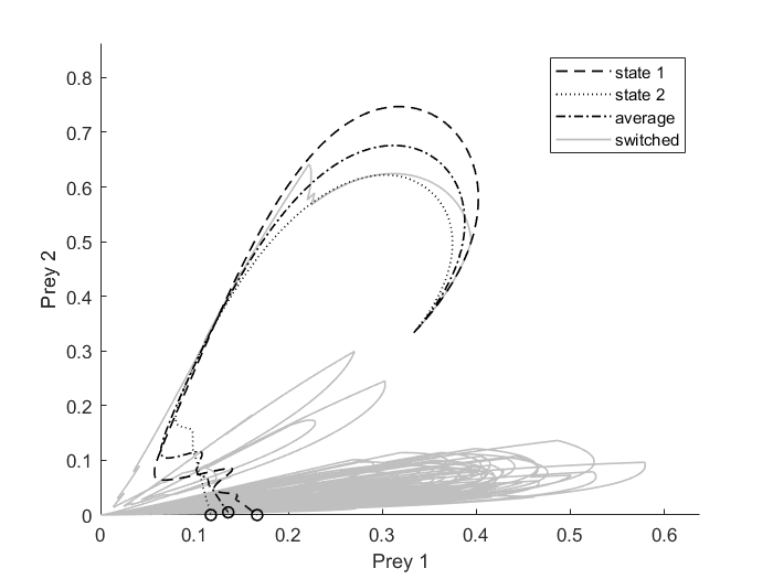
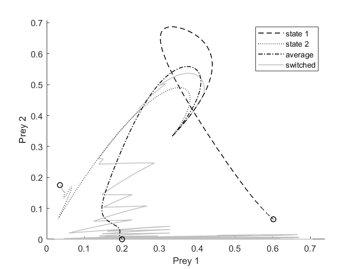
Figure 1. Trajectories in prey 1 - prey 2 phase space. All simulations in a given panel have the same initial conditions. Small circles denote the fixed points for the various vector fields. Left panel: (Example 5.1) In each fixed environmental state prey 2 goes extinct. Switching makes all three species coexist. Right panel: (Example 5.2) In each fixed environmental state the three species coexist. Prey 2 goes extinct in the switched system.

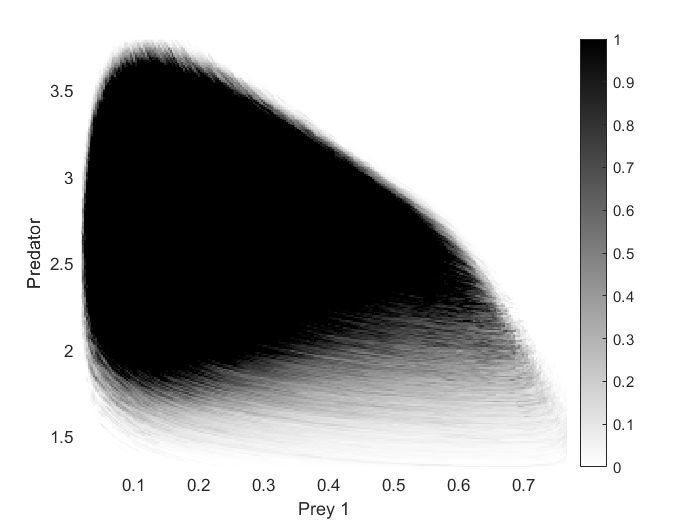
(a) State 1

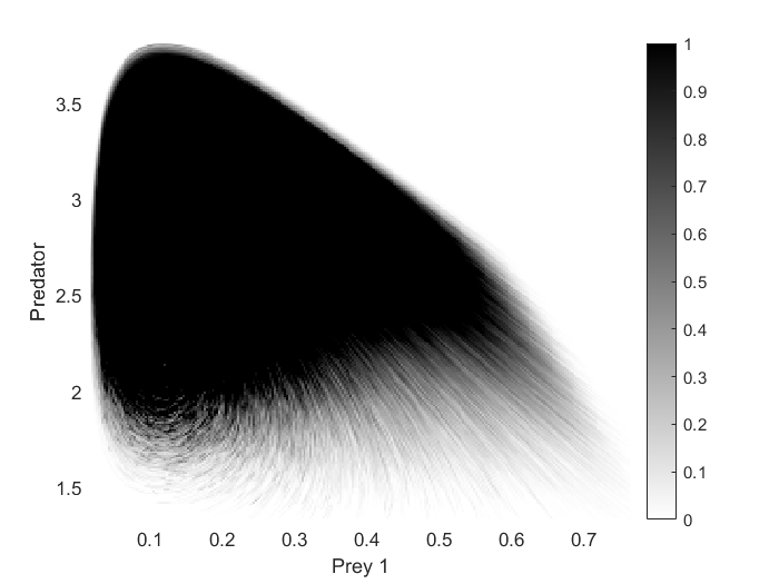
(b) State 2

Figure 2. (Example 5.2) The joint density of $X_{1}=\text{Prey 1}$ and $X_{3}=\text{Predator}$ in state 1 and state 2 was simulated 100 times on the time interval $[0,10000]$ for a solution $(X_{1},X_{2},X_{3})$ initial values $(2/3,2/3,3/2).$ The occupation measure for the switched system converges exponentially fast to the absolutely continuous invariant measure on $\mathbb{R}^{13,\circ}_{+}$.

Example 5.2.

Consider the parameters

$$\begin{cases}r=1,\hskip 10.00002ptd=0.1\\ b_{1}=0.9,\hskip 10.00002ptb_{2}=0.5\\ c_{1}(1)=0.15,\hskip 10.00002ptc_{1}(2)=0.4\\ c_{2}(1)=0.28,\hskip 10.00002ptc_{1}(2)=0.4\\ e_{1}(1)=0.15,\hskip 10.00002pte_{1}(2)=0.85\\ e_{2}(1)=0.15,\hskip 10.00002pte_{2}(2)=0.4.\\ \end{cases}$$

Then

$$\begin{cases}\lambda_{1}(\delta_{13},1)\approx 0.1333,\\ \lambda_{1}(\delta_{13},2)\approx 0.0667,\\ \lambda_{1}(\delta_{23},1)\approx 0.6643,\\ \lambda_{1}(\delta_{23},2)\approx 0.0333,\\ \end{cases}$$

and

$$\begin{cases}r-\frac{d}{\overline{e_{1}}}b_{2}-(r-\frac{d}{\overline{e_{1}}})\frac{\overline{c_{2}}}{\overline{c_{1}}}\approx-0.1114,\\ r-\frac{d}{\overline{e_{2}}}b_{1}-(r-\frac{d}{\overline{e_{2}}})\frac{\overline{c_{1}}}{\overline{c_{2}}}\approx 0.2483.\end{cases}$$

This shows that the equilibrium point in the interior $\mathbb{R}^{3,\circ}_{+}$ is asymptotically stable for both deterministic systems corresponding to state 1 and state 2. The three species coexist in both environments, if there is no randomness. However, when the switching is fast, one has $\lambda_{2}(\mu_{13})\approx r-\frac{d}{\overline{e_{1}}}b_{2}-(r-\frac{d}{\overline{e_{1}}})\frac{\overline{c_{2}}}{\overline{c_{1}}}<0$ and $\lambda_{1}(\mu_{23})\approx r-\frac{d}{\overline{e_{2}}}b_{1}-(r-\frac{d}{\overline{e_{2}}})\frac{\overline{c_{1}}}{\overline{c_{2}}}>0$. Using Theorem 4 we see that in the random system, prey 1 and the predator persist, while prey 2 can go extinct with a large probability when it starts at a small initial density (see Figure 1 and Figure 2).

Acknowledgments: The authors acknowledge support from the NSF through the grants DMS-1853463 for Alexandru Hening and DMS-1853467 for Dang Nguyen.

References

• (1)
• Bakhtin & Hurth (2012) Bakhtin, Y. & Hurth, T. (2012), ‘Invariant densities for dynamical systems with random switching’, Nonlinearity 25(10), 2937.
• Benaïm (2018) Benaïm, M. (2018), ‘Stochastic persistence’. preprint.
• Benaïm et al. (2008) Benaïm, M., Hofbauer, J. & Sandholm, W. H. (2008), ‘Robust permanence and impermanence for stochastic replicator dynamics’, J. Biol. Dyn. 2(2), 180–195.
• Benaïm et al. (2015) Benaïm, M., Le Borgne, S., Malrieu, F. & Zitt, P.-A. (2015), Qualitative properties of certain piecewise deterministic markov processes, in ‘Annales de l’IHP Probabilités et statistiques’, Vol. 51, pp. 1040–1075.
• Benaïm & Lobry (2016) Benaïm, M. & Lobry, C. (2016), ‘Lotka Volterra in fluctuating environment or “how switching between beneficial environments can make survival harder”’, Ann. Appl. Probab. . to appear.
• Benaïm & Schreiber (2009) Benaïm, M. & Schreiber, S. J. (2009), ‘Persistence of structured populations in random environments’, Theoretical Population Biology 76(1), 19–34.
• Chesson (2000) Chesson, P. (2000), ‘General theory of competitive coexistence in spatially-varying environments’, Theoretical Population Biology 58(3), 211–237.
• Chesson (1982) Chesson, P. L. (1982), ‘The stabilizing effect of a random environment’, Journal of Mathematical Biology 15(1), 1–36.
• Chesson & Ellner (1989) Chesson, P. L. & Ellner, S. (1989), ‘Invasibility and stochastic boundedness in monotonic competition models’, Journal of Mathematical Biology 27(2), 117–138.
• Davis (1984) Davis, M. H. A. (1984), ‘Piecewise-deterministic markov processes: A general class of non-diffusion stochastic models’, Journal of the Royal Statistical Society: Series B (Methodological) 46(3), 353–376.
• Du & Dang (2014) Du, N. H. & Dang, N. H. (2014), ‘Asymptotic behavior of kolmogorov systems with predator-prey type in random environment’, Communications on Pure & Applied Analysis 13(6), 2693.
• Ethier & Kurtz (2009) Ethier, S. N. & Kurtz, T. G. (2009), Markov processes: characterization and convergence, Vol. 282, John Wiley & Sons.
• Evans et al. (2015) Evans, S. N., Hening, A. & Schreiber, S. J. (2015), ‘Protected polymorphisms and evolutionary stability of patch-selection strategies in stochastic environments’, J. Math. Biol. 71(2), 325–359.
• Evans et al. (2013) Evans, S. N., Ralph, P. L., Schreiber, S. J. & Sen, A. (2013), ‘Stochastic population growth in spatially heterogeneous environments’, J. Math. Biol. 66(3), 423–476.
• Hardin (1960) Hardin, G. (1960), ‘The competitive exclusion principle’, science 131(3409), 1292–1297.
• Hening, Nguyen & Chesson (2021) Hening, A., Nguyen, D. & Chesson, P. (2021), ‘A general theory of coexistence and extinction for stochastic ecological communities’, Journal of Mathematical Biology 82(6), 1–76.
• Hening & Nguyen (2018) Hening, A. & Nguyen, D. H. (2018), ‘Coexistence and extinction for stochastic Kolmogorov systems’, Ann. Appl. Probab. 28(3), 1893–1942.
• Hening & Nguyen (2020) Hening, A. & Nguyen, D. H. (2020), ‘The competitive exclusion principle in stochastic environments’, Journal of Mathematical Biology 80, 1323––1351.
• Hening, Nguyen & Schreiber (2021) Hening, A., Nguyen, D. H. & Schreiber, S. J. (2021), ‘A classification of the dynamics of three-dimensional stochastic ecological systems’, Annals of Applied Probability .
• Hening & Strickler (2019) Hening, A. & Strickler, E. (2019), ‘On a predator-prey system with random switching that never converges to its equilibrium’, SIAM Journal on Mathematical Analysis 51(5), 3625–3640.
• Hutchinson (1961) Hutchinson, G. E. (1961), ‘The paradox of the plankton’, The American Naturalist 95(882), 137–145.
• Hutson & Vickers (1983) Hutson, V. & Vickers, G. T. (1983), ‘A criterion for permanent coexistence of species, with an application to a two-prey one-predator system’, Mathematical Biosciences 63(2), 253–269.
• Lande et al. (2003) Lande, R., Engen, S. & Saether, B.-E. (2003), Stochastic population dynamics in ecology and conservation, Oxford University Press on Demand.
• Levin (1970) Levin, S. A. (1970), ‘Community equilibria and stability, and an extension of the competitive exclusion principle’, The American Naturalist 104(939), 413–423.
• Paine (1966) Paine, R. T. (1966), ‘Food web complexity and species diversity’, The American Naturalist 100(910), 65–75.
• Schreiber (1997) Schreiber, S. J. (1997), ‘Generalist and specialist predators that mediate permanence in ecological communities’, Journal of Mathematical Biology 36(2), 133–148.
• Schreiber et al. (2011) Schreiber, S. J., Benaïm, M. & Atchadé, K. A. S. (2011), ‘Persistence in fluctuating environments’, J. Math. Biol. 62(5), 655–683.
• Schreiber & Lloyd-Smith (2009) Schreiber, S. J. & Lloyd-Smith, J. O. (2009), ‘Invasion dynamics in spatially heterogeneous environments’, The American Naturalist 174(4), 490–505.
• Takeuchi & Adachi (1983) Takeuchi, Y. & Adachi, N. (1983), ‘Existence and bifurcation of stable equilibrium in two-prey, one-predator communities’, Bulletin of mathematical Biology 45(6), 877–900.
• Tuong et al. (2019) Tuong, T., Nguyen, D. H., Dieu, N. & Tran, K. (2019), ‘Extinction and permanence in a stochastic sirs model in regime-switching with general incidence rate’, Nonlinear Analysis: Hybrid Systems 34, 121–130.
• Volterra (1928) Volterra, V. (1928), ‘Variations and fluctuations of the number of individuals in animal species living together’, J. Cons. Int. Explor. Mer 3(1), 3–51.
• Watts et al. (2021) Watts, H., Mishra, A., Nguyen, D. H. & Tuong, T. D. (2021), ‘Dynamics of a vector-host model under switching environments’, Discrete & Continuous Dynamical Systems-B .