Robust Accelerated Primal-Dual Methods for Computing Saddle Points

Abstract

We consider strongly-convex-strongly-concave saddle point problems assuming we have access to unbiased stochastic estimates of the gradients. We propose a stochastic accelerated primal-dual (SAPD) algorithm and show that SAPD sequence, generated using constant primal-dual step sizes, linearly converges to a neighborhood of the unique saddle point. Interpreting the size of the neighborhood as a measure of robustness to gradient noise, we obtain explicit characterizations of robustness in terms of SAPD parameters and problem constants. Based on these characterizations, we develop computationally tractable techniques for optimizing the SAPD parameters, i.e., the primal and dual step sizes, and the momentum parameter, to achieve a desired trade-off between the convergence rate and robustness on the Pareto curve. This allows SAPD to enjoy fast convergence properties while being robust to noise as an accelerated method. SAPD admits convergence guarantees for the distance metric with a variance term optimal up to a logarithmic factor –which can be removed by employing a restarting strategy. We also discuss how convergence and robustness results extend to the convex-concave setting. Finally, we illustrate our framework on distributionally robust logistic regression problem.

1 Introduction

We consider the following saddle point (SP) problem:

$$\min_{x\in\mathcal{X}}\max_{y\in\mathcal{Y}}\mathcal{L}(x,y)\triangleq f(x)+\Phi(x,y)-g(y),$$ (1)

where $\mathcal{X}$ and $\mathcal{Y}$ are, $n$ and $m$ dimensional inner product spaces endowed with inner product norms $\|x\|_{\mathcal{X}}=\sqrt{\langle x,x\rangle}_{\mathcal{X}}$ and $\|y\|_{\mathcal{Y}}=\sqrt{\langle y,y\rangle}_{\mathcal{Y}}$, respectively; $\Phi:\mathcal{X}\times\mathcal{Y}\rightarrow\mathbb{R}$ is convex in $x$, concave in $y$ with a Lipschitz gradient; $f:\mathcal{X}\rightarrow\mathbb{R}{\color[rgb]{0,0,0}\cup\{{\color[rgb]{0,0,0}+}\infty\}}$ and $g:\mathcal{Y}\rightarrow\mathbb{R}{\color[rgb]{0,0,0}\cup\{{\color[rgb]{0,0,0}+}\infty\}}$ are closed, convex functions. We assume that $\mathcal{L}(x,y)$ is (strongly) convex in $x$ and (strongly) concave in $y$ with moduli $\mu_{x},\mu_{y}\geq 0$, respectively. The SP problem in (1) has a wide range of applications; in fact, many convex optimization problems arising in machine learning (ML) can be recast as (1) through Lagrangian duality. Prominent applications with SP formulations include empirical risk minimization (ERM) [53, 42], supervised learning with non-separable losses, or regularizers [46, 38], distributionally robust ERM [29], and robust optimization [4]. In many of these applications, one does not have access to exact values of the gradients $\nabla_{x}\Phi$ and $\nabla_{y}\Phi$; but, rather has access to their unbiased stochastic estimates $\tilde{\nabla}_{x}\Phi$ and $\tilde{\nabla}_{y}\Phi$. This would typically be the case when the gradients are estimated from a subset of data points in the big-data regime (as in stochastic gradient, and stochastic approximation methods) or if noise is injected to the gradients on purpose to protect the privacy of the user data [45].

We propose a first-order method, the Stochastic Accelerated Primal-Dual (SAPD) algorithm, to solve (1) under the assumption that we have access to unbiased stochastic oracles $\tilde{\nabla}_{x}\Phi$ and $\tilde{\nabla}_{y}\Phi$ with a bounded variance, see Assumption 2 for the details. This setting is commonly considered in the literature and is relevant to a number of applications, e.g., training GANs [55] and robust learning [44]. First, assuming that $\mathcal{L}$ is strongly convex strongly concave (SCSC), we show that SAPD sequence, generated using constant primal-dual step sizes, linearly converges to a neighborhood of the unique saddle point. Interpreting the size of the neighborhood as a measure of robustness to gradient noise, we propose computationally tractable techniques for optimizing the SAPD parameters to achieve a desired trade-off between the convergence rate and robustness. We also discuss how convergence and robustness results extend to the convex-concave setting with $\mu_{x}=\mu_{y}=0$.

1.1 Related Work

When the coupling term $\Phi(x,y)$ is bilinear, i.e., $\Phi(x,y)=\langle Kx,y\rangle$ for some linear operator $K:\mathcal{X}\rightarrow{\color[rgb]{0,0,0}\mathcal{Y}^{*}}$, (1) is well-studied for both strongly-convex-strongly-concave (SCSC) problems ($\mu_{x},\mu_{y}>0$) as well as for merely-convex-merely-concave (MCMC) problems ($\mu_{x}=\mu_{y}=0$). The convergence results cover both the stochastic case (when only stochastic estimates of the gradients are available) and the deterministic case (when the gradient information is exact). In our work, we do not assume bilinear $\Phi$. When the coupling term $\Phi$ is non-bilinear, there exist some convergence results in the deterministic case; however, the stochastic setting remains relatively understudied. Two standard metrics to measure the quality of a random $(\bar{x},\bar{y})\in\mathcal{X}\times\mathcal{Y}$ returned by a stochastic algorithm are the gap function $\mathcal{G}:\mathcal{X}\times\mathcal{Y}\to\mathbb{R}_{+}$ for the MCMC case and distance metric $\mathcal{D}:\mathcal{X}\times\mathcal{Y}\to\mathbb{R}_{+}$ for the SCSC case, for which there is a unique saddle point $(x^{*},y^{*})$, i.e.,

$$\mathcal{G}(\bar{x},\bar{y})\triangleq\mathbb{E}\big{[}\sup_{(x,y)\in\mathcal{X}\times\mathcal{Y}}\big{\{}\mathcal{L}(\bar{x},y)-\mathcal{L}(x,\bar{y})\big{\}}\big{]},\quad{\color[rgb]{0,0,0}\mathcal{D}(\bar{x},\bar{y})\triangleq\mathbb{E}[\mu_{x}\|\bar{x}-x^{*}\|^{2}+\mu_{y}\|\bar{y}-y^{*}\|^{2}]},\vspace*{-2mm}$$ (2)

where the expectation is taken with respect to the randomness encountered in the generation of the point $(\bar{x},\bar{y})\in\mathcal{X}\times\mathcal{Y}$. In the following discussion, we summarize existing results closely related to our setting, and discuss our contributions.

1.1.1 The Deterministic Case

The bilinear structure has been thoroughly studied; some well-known algorithms include excessive gap technique [34, 33], primal-dual hybrid gradient (PDHG) [7, 8] –also see [41] achieving the best bound. On the other extreme, when $\mathcal{L}$ owns a general form and the smoothness cannot be guaranteed, primal-dual subgradient algorithms have been proposed in several works, e.g., [30, 35, 21]. The iteration complexity of these subgradient-based methods can be significantly improved when $\mathcal{L}$ has further structure. Indeed, there are methods exploiting the structure when $\Phi$ is smooth, and $f,g$ have efficient prox maps, which include Mirror-Prox(MP) [31], Optimistic Gradient Descent Ascent (OGDA) and Extra-gradient (EG) [28] methods. Additionally, the effect of Lipschitz constants along different blocks of variables also has been explored recently; some new works account for the individual effects of $L_{xx}$, $L_{yx}$ and $L_{yy}$, i.e., the Lipschitz constants of $\nabla_{x}\Phi(\cdot,y)$, $\nabla_{y}\Phi(x,\cdot)$ and $\nabla_{y}\Phi(\cdot,y)$, respectively, instead of using the worst-case parameters $L\triangleq\max\{L_{xx},L_{xy},L_{yx},{\color[rgb]{0,0,0}L_{yy}}\}$, $\mu\triangleq\min\{\mu_{x},\mu_{y}\}$. For bilinear SP problems, a lower complexity bound of ${{\Omega}\Big{(}\sqrt{1+\frac{L_{yx}^{2}}{\mu_{x}\mu_{y}}}\cdot\ln(1/\epsilon)\Big{)}}$ is shown in [49] for a class of first-order primal-dual algorithms employing proximal-gradient steps; on the other hand, the lower bound for gradient-based methods is $\Omega\Big{(}\sqrt{\frac{L_{xx}}{\mu_{x}}+\frac{L_{yx}^{2}}{\mu_{x}\mu_{y}}+\frac{L_{yy}}{\mu_{y}}}\cdot\ln(1/\epsilon)\Big{)}$ when $f(\cdot)=g(\cdot)=0$ and $\Phi$ is SCSC [49]. In the rest, we focus on the deterministic SCSC setup, for which the results in $\mathcal{D}$ metric can be converted into gap metric $\mathcal{G}$ by only increasing the logarithmic term by problem parameters, see [10, Appendix C].

Mokhtari et al. [28] show that both OGDA and EG have an iteration complexity of $\mathcal{O}\Big{(}\frac{L}{\mu}\ln(1/\varepsilon)\Big{)}$ for $\mathcal{D}$ metric defined in (2). Gidel et al. [15] also show the same rate for OGDA from a variational inequality (VI) perspective. In the analysis of these algorithms, primal and dual step sizes are set equal, which may lead to conservative steps whenever $L_{xx}\gg L_{yy}$, or vice versa. For instance, in the primal-dual formulation of empirical risk minimization problems in machine learning, choosing primal and dual step sizes to be different can lead to an improved convergence rate [53]. There are also some multi-loop algorithms. In particular, Lin et al. [26] proposed an inexact proximal point algorithm, which consists of 3-nested loops. Indeed, each proximal step computation requires calling Nesterov’s accelerated gradient descent (AGD) iteratively to solve strongly convex smooth (SCS) optimization subproblems with a high precision that can be impractical. The computational complexity to compute $(\bar{x},\bar{y})$ such that $\mathcal{G}(\bar{x},\bar{y})\leq\epsilon$ is $\mathcal{O}\left(\frac{L}{\sqrt{\mu_{x}\mu_{y}}}\cdot{\color[rgb]{0,0,0}\ln^{3}}(1/\epsilon)\right)$. Although [26] claims to achieve the lower complexity bound provided in [49], this is not the case for problems with $L_{yx}\ll L$. The algorithm in [43] consists of 4-nested loops and has similar shortcomings in practice. The computational complexity to compute $(\bar{x},\bar{y})$ such that $\mathcal{D}(\bar{x},\bar{y})\leq\epsilon$ is $\mathcal{O}(\sqrt{\frac{L_{xx}}{\mu_{x}}+\frac{LL_{xy}}{\mu_{x}\mu_{y}}+\frac{L_{yy}}{\mu_{y}}}\cdot\ln^{3}(1/\epsilon))$. More recently, after our preprint [51] has appeared, Jin el al. [20] independently obtain the iteration complexity of ${\mathcal{O}}\Big{(}\big{(}\frac{L_{xx}}{\mu_{x}}+\frac{L_{yx}}{\sqrt{\mu_{x}\mu_{y}}}+\frac{L_{yy}}{\mu_{y}}\big{)}\cdot\ln(1/\epsilon)\Big{)}$ for satisfying $\mathcal{G}(\bar{x},\bar{y})\leq\epsilon$.

1.1.2 The Stochastic Case

While the deterministic SP problem has attracted much attention, the study on the first-order stochastic methods for (1) is still relatively limited. For MCMC SP problems, proximal methods have been developed, e.g., Stochastic Mirror-Descent(SMD) [32], the Stochastic Mirror-Prox (SMP) [22] and its accelerated version (SAMP) [9]. In [54], MCMC and strongly-convex-merely-concave (SCMC) scenarios are considered under additive unbiased noise with a bounded variance. When $\mu_{x}>0$, a multi-stage scheme achieving the best known complexity for the stochastic SP problems is proposed in [54]; however, this is a two-loop method and each outer iteration requires solving a non-trivial sub-problem with an increasing accuracy, which is a function of some problems parameters that may not be known in practice, e.g., Bregman diameters of $\mathcal{X},\mathcal{Y}$ and noise variance. There are also some VI-based methods [12, 15] for the MCMC scenario.

Our focus in this paper will be on the stochastic SCSC case. Yan et al. [47] consider $\min_{x\in X}\max_{y\in Y}\Phi(x,y)$ for possibly non-smooth, SCSC $\Phi$, and propose Epoch-GDA with an oracle complexity of $\mathcal{O}\left(\frac{1}{\epsilon}\ln(1/p)\right)$ for computing $(\bar{x},\bar{y})$ such that $\mathcal{G}(\bar{x},\bar{y})\leq\epsilon$ with probability $1-p$. When $\Phi$ is smooth, stochastic EG method [19] for SCSC SP problems and Stochastic Operator Extrapolation method [24] for strongly monotone VIs, both using constant step sizes, can guarantee $\mathcal{D}(x_{k},y_{k})\leq\epsilon$ within $\mathcal{O}\left(\frac{1}{\epsilon}\right)$ and $\mathcal{O}(\kappa\ln(1/\epsilon)+\tfrac{\delta^{2}}{\mu\epsilon}\ln(1/\epsilon))$ iterations, respectively, where $\kappa=L/\mu$. Fallah et al. [13] propose multi-stage variants (employing restarts) of Stochastic Gradient Descent Ascent (S-GDA) and Stochastic OGDA (S-OGDA) that can guarantee $\mathcal{D}(x_{k},y_{k})\leq\epsilon$ within $\mathcal{O}(\kappa^{2}\ln(1/\epsilon)+\tfrac{\delta^{2}}{\mu\epsilon})$ and $\mathcal{O}(\kappa\ln(1/\epsilon)+\tfrac{\delta^{2}}{\mu\epsilon})$ iterations, respectively. Unlike our paper, in both [19, 13], Lipschitz constant of $\nabla\Phi$, i.e., $L$, is used to determine the step size, rather than exploiting the block Lipschitz structure.

1.2 Comparison

Method	Bias	Variance	Loop	Metric	BV-tradeoff
[26]	$\frac{L}{\sqrt{\mu_{x}\mu_{y}}}\ln^{3}\big{(}\frac{1}{\epsilon}\big{)}$	✗	3	$\mathcal{G}$	N/A
[43]	$\tilde{\mathcal{O}}\Big{(}\big{(}{\frac{L_{xx}}{\mu_{x}}}+\frac{L\cdot L_{xy}}{\mu_{x}\mu_{y}}+{\frac{L_{yy}}{\mu_{y}}}\big{)}^{1/2}\Big{)}{\ln\left(\frac{1}{\epsilon}\right)}$	✗	4	$\mathcal{D}$	N/A
[48]	$\frac{L}{\mu}\ln(\frac{1}{\epsilon})$	✗	2	$\mathcal{D}$	N/A
[28]	$\frac{L}{\mu}\ln(\frac{1}{\epsilon})$	✗	1	$\mathcal{D}$	N/A
[10, 20]	$(\frac{L_{xx}}{\mu_{x}}+{\frac{L_{yx}}{\sqrt{\mu_{x}\mu_{y}}}}+\frac{L_{yy}}{\mu_{y}}){\ln(\frac{1}{\epsilon})}$	✗	1	$\mathcal{G}$	N/A
[47]	$\tilde{\mathcal{O}}(\frac{1}{\epsilon}\ln(1/p))$	$\tilde{\mathcal{O}}(\frac{\delta^{2}}{\mu\epsilon}\ln(1/p))$	2	$\mathcal{P}_{p}$	✗
[13]	$\frac{L}{\mu}\ln(\frac{1}{\epsilon})$	$\frac{\delta^{2}}{\mu\epsilon}$	2	$\mathcal{D}$	✗
[19]	$\frac{1}{\epsilon}$	$\frac{\delta^{2}}{\mu\epsilon}$	1	$\mathcal{D}$	✗
ours	$(\frac{L_{xx}}{\mu_{x}}+{\frac{L_{yx}}{\sqrt{\mu_{x}\mu_{y}}}}+\frac{L_{yy}}{\mu_{y}}){\ln(\frac{1}{\epsilon})}$	${(\frac{\delta_{x}^{2}}{\mu_{x}}+\frac{\delta_{y}^{2}}{\mu_{y}})\frac{1}{\epsilon}}\ln(\frac{1}{\epsilon})$	1	$\mathcal{D}$	✔

Table 1: Related work: Comparison of methods for solving SCSC saddle point problem in (1) with a non-bilinear $\Phi$. [10] requires $\Phi$ to be twice differentiable. Results in $\mathcal{D}$ metric can be converted into guarantees in the gap metric $\mathcal{G}$ while still preserving $\ln(1/\epsilon)+1/\epsilon$ complexity, see [10, Appendix C]. The metric $\mathcal{P}_{p}$ denotes the number of oracle calls for $\mathcal{G}\leq\epsilon$ with probability at least $1-p$. Among single-loop methods, [28] employs $\tau=\sigma=\frac{1}{4L}$, [10] employs $\tau=\frac{1}{\mu_{x}\lambda}$ and $\sigma=\frac{1}{\mu_{y}\lambda}$, where $\lambda=\frac{L_{xx}}{\mu_{x}}+\frac{L_{xy}}{\sqrt{\mu_{x}\mu_{y}}}+\frac{L_{yy}}{\mu_{y}}$, [19] employs $\tau_{k}=\sigma_{k}=\frac{1}{\alpha k+4L}$ for $\alpha\in(0,\mu)$. In the column “BV-tradeoff” we indicated whether a systematic analysis is provided for the bias-variance trade-off.

In table 1, among the papers we discuss in section 1.1 we compare the deterministic and stochastic methods for solving the SCSC saddle point problem in (1) with a non-bilinear $\Phi$ –to focus on more relevant papers, we did not include methods for $\Phi$ that is bilinear and/or in the finite-sum form. For deterministic methods, having access to $\nabla_{x}\Phi$ and $\nabla_{y}\Phi$, we only provide the bias term of the oracle complexity –this term represents the work required against the bias introduced due to initialization of the algorithm while computing an $\epsilon$-solution. For methods employing stochastic first-order oracles (SFO) to get noisy estimates $\tilde{\nabla}_{x}\Phi$ and $\tilde{\nabla}_{y}\Phi$, we provide both the bias and variance terms in the oracle complexity result, where variance term denotes the additional oracle calls required due to persistent noise in gradient estimates compared to the (noiseless) deterministic case. For all the methods compared, we list how many nested loops they employ. Finally, in the last column “BV-tradeoff” of Table 1 we indicate whether a systematic analysis is provided for the bias-variance trade-off for the stochastic methods discussed in the table. While our paper is achieving near optimal state-of-the art complexities for both bias and variance as a single loop method, it also provides conditions on algorithm parameters describing the dependency between the parameter choice and corresponding certifiable rate –see (5); hence, our admissibility rule allows us to characterize the bias-variance trade-off for the SAPD algorithm.

1.3 Contributions

We propose the Stochastic Accelerated Primal-Dual (SAPD) algorithm which extends APD method proposed in [18] to the stochastic gradient setting. We assume that the first-order oracles $\tilde{\nabla}\Phi_{x}$ and $\tilde{\nabla}\Phi_{y}$ return noisy partial gradients that are unbiased and have finite variance bounded by $\delta_{x}^{2}$ and $\delta_{y}^{2}$, respectively. Let $z^{*}=(x^{*},y^{*})$ denote the unique saddle point of the SCSC minimax problem in (1). For any $\epsilon>0$, SAPD guarantees $\mathcal{D}({x}_{N},{y}_{N})\leq\epsilon$ within

$$N\leq\mathcal{O}\Big{(}\Big{(}\frac{L_{xx}}{\mu_{x}}+\frac{L_{yx}}{\sqrt{\mu_{x}\mu_{y}}}+\frac{L_{yy}}{\mu_{y}}+\Big{(}\frac{\delta_{x}^{2}}{{\color[rgb]{0,0,0}\mu_{x}}}+\frac{\delta_{y}^{2}}{{\color[rgb]{0,0,0}\mu_{y}}}\Big{)}\frac{1}{\epsilon}\Big{)}\cdot\ln\Big{(}\frac{{\color[rgb]{0,0,0}\mathcal{D}(x_{0},y_{0})}}{\epsilon}\Big{)}\Big{)}\vspace*{-2mm}$$

iterations. The oracle complexity bound on the bias term $\mathcal{O}(\kappa\ln(1/\epsilon))$ is optimal, where $\kappa=L/\mu$, and the bound on the variance term $\tilde{\mathcal{O}}((\delta_{x}^{2}/{\color[rgb]{0,0,0}\mu_{x}}+\delta_{y}^{2}/{\color[rgb]{0,0,0}\mu_{y}})/\epsilon)$ is optimal up to a log factor, which can be removed by employing a restarting strategy as in [13] –see appendix D for details. Since the noise is persistent, linear convergence cannot be achieved – unlike the finite sum problems where variance reduction-based methods are applicable to obtain linear convergence [38]. However, for SCSC problems, SAPD with constant step size converges to a neighborhood of the saddle-point at a linear rate $\rho\in(0,1)$, and the size of the neighborhood, defined as $\limsup_{N\to\infty}\mathbb{E}[\|z_{N}-z^{*}\|^{2}]$, scales linearly with the gradient noise level; hence, we interpret the ratio $\limsup_{N\to\infty}\mathbb{E}[\|z_{N}-z^{*}\|^{2}]/\delta^{2}$ as a measure of robustness, which we denote with $\mathcal{J}$, where $\delta^{2}=\max\{\delta^{2}_{x},\delta^{2}_{y}\}$. We evaluate the overall algorithmic performance with two metrics: SAPD parameters should be tuned to achieve a faster rate $\rho$ with a smaller noise amplification $\mathcal{J}$. Our analysis leads to explicit characterizations of $\mathcal{J}$ for a particular problem class, and of an upper bound $\mathcal{R}$ on $\mathcal{J}$ for more general problems; both $\mathcal{J}$ and $\mathcal{R}$ are given as functions of SAPD parameters. Based on these characterizations, we develop computationally tractable techniques for optimizing the SAPD parameters to achieve a desired systematic trade-off between $\rho$ and $\mathcal{J}$ without assuming the knowledge of noise variance bounds, $\delta^{2}_{x}$ and $\delta^{2}_{y}$. This allows SAPD to enjoy fast convergence with a robust performance in the presence of stochastic gradient noise. Achieving systematic trade-offs between the rate and robustness has been previously studied in [2] in the context of accelerated methods for smooth strongly convex minimization problems. To our knowledge, our work is the first one that can trade-off $\rho$ with $\mathcal{J}$ in a systematic fashion in the context of primal-dual algorithms for (1).

For the stochastic MCMC case, SAPD can generate $(\bar{x},\bar{y})$ such that $\mathcal{G}(\bar{x},\bar{y})\leq\epsilon$ within $\mathcal{O}(L/\epsilon+\delta^{2}/\epsilon^{2})$ oracle calls, which is optimal for this setting in both bias and variance terms. For both SCSC and MCMC scenarios, the deterministic results can be derived from our stochastic results immediately by setting the noise variances $\delta_{x}^{2}=\delta_{y}^{2}=0$. In the deterministic setting, our algorithm, when applied to (1) with a bilinear $\Phi$, generates the same iterate sequence with [8] for a specific choice of step size parameters; therefore, SAPD, being able to handle noisy gradients and non-bilinear couplings, can be viewed as a general form of the optimal method (CP) proposed by Chambolle and Pock [8] for MCMC and SCSC problems with a bilinear coupling. Indeed, in the deterministic case when $\Phi$ is bilinear, both CP and SAPD hit the lower complexity bounds, $\Omega(L/\epsilon)$ for the MCMC and $\Omega(\frac{L_{yx}}{\sqrt{\mu_{x}\mu_{y}}}\ln(1/\epsilon))$ for the SCSC problems, given in [37] and [49], respectively. Moreover, when $\Phi$ is not assumed to be bilinear, SAPD guarantees $\mathcal{O}(L/\epsilon)$ complexity in the MCMC setting and $\mathcal{O}((\frac{L_{xx}}{\mu_{x}}+\frac{L_{yy}}{\mu_{y}}+\frac{L_{yx}}{\sqrt{\mu_{x}\mu_{y}}})\cdot\ln(1/\epsilon))$ complexity in the SCSC setting for the bias term, which are the best bounds shown for (1). For the SCSC setup, the papers [10, 20] provide bias guarantees similar to our method; but, they are not applicable to the (noisy) stochastic setting like ours. Furthermore, our framework exploiting block Lipschitz constants $L_{xx}$, $L_{yx}$ and $L_{yy}$, provides larger step sizes compared to the traditional step size $\mathcal{O}(1/L)$.

Finally, the single-loop design of our algorithm make it suitable for solving large-scale problems efficiently –usually in methods with nested loops, inner iterations are terminated when a sufficient optimality condition holds and these conditions are usually very conservative, leading to excessive number of inner iterations. Furthermore, solving nonconvex-convex minimax problems using an inexact proximal point method requires solving SCSC subproblems to an increasing accuracy; hence, adopting single-loop algorithms as solvers for SCSC subproblems leads to simple implementations compared to using multi-loop methods as solvers –see [52]. Indeed, single loop algorithms are preferable compared to multi-loop algorithms in many settings, e.g., see [50] for a discussion.

1.4 Notation

Throughout the paper, $\mathbb{R}_{++}$ denotes the set of positive real numbers, and $\mathbb{R}_{+}=\mathbb{R}_{++}\cup\{\mathbf{0}\}$. We adopted arithmetic using the extended reals with the convention that $\frac{1}{0}\triangleq\infty$, $\frac{0^{2}}{0}\triangleq 0$, $\frac{0}{0^{2}}\triangleq\infty$. We use $\|\cdot\|$ to denote the Euclidean norm. The proximal operator associated with a proper, closed convex $f:\mathcal{X}\to\mathbb{R}\cup\{\infty\}$ is given by $\mathbf{prox}_{f}(x)\triangleq\operatorname*{\textbf{argmin}}_{v\in\mathcal{X}}f(v)+{\frac{1}{2}}\|x-v\|^{2}$, and $\mathbf{prox}_{g}(\cdot)$ is defined similarly. We let $\mathbb{S}^{d}$ denote the set of symmetric $d\times d$ real matrices.

1.5 Assumptions and Statement of SAPD Algorithm

In the following, we introduce the assumptions needed throughout this paper.

Assumption 1.

$f:\mathcal{X}\rightarrow\mathbb{R}{\color[rgb]{0,0,0}\cup\{{\color[rgb]{0,0,0}+}\infty\}}$ and $g:\mathcal{Y}\rightarrow\mathbb{R}{\color[rgb]{0,0,0}\cup\{{\color[rgb]{0,0,0}+}\infty\}}$ are proper, closed, convex functions with moduli $\mu_{x},\mu_{y}\geq 0$. Moreover, $\Phi:\mathcal{X}\times\mathcal{Y}\to\mathbb{R}$ is such that

(i) for any $y\in\mathop{\bf dom}g\subset\mathcal{Y}$, $\Phi(\cdot,y)$ is convex and differentiable; and $\exists L_{xx}\geq 0$, $\exists L_{xy}>0$ such that $\forall x,\bar{x}\in\mathop{\bf dom}f\subset\mathcal{X}$ and $\forall y,\bar{y}\in\mathop{\bf dom}g\subset\mathcal{Y}$,

$$\|\nabla_{x}\Phi(x,y)-\nabla_{x}\Phi(\bar{x},\bar{y})\|\leq L_{xx}\|x-\bar{x}\|+L_{xy}\|y-\bar{y}\|;$$ (3)

(ii) for any $x\in\mathop{\bf dom}f\subset\mathcal{X}$, $\Phi(x,\cdot)$ is concave and differentiable; and $\exists$ $L_{yx}{>}0$ and ${\color[rgb]{0,0,0}\exists}L_{yy}\geq 0$ such that $\forall x,\bar{x}\in\mathop{\bf dom}f\subset\mathcal{X}$ and $\forall y,\bar{y}\in\mathop{\bf dom}g\subset\mathcal{Y}$,

$$\|\nabla_{y}\Phi(x,y)-\nabla_{y}\Phi(\bar{x},\bar{y})\|\leq L_{yx}\|x-\bar{x}\|+L_{yy}\|y-\bar{y}\|.$$ (4)

Remark 1.

In fact, in terms of strong convexity, we only need to assume that $\mathcal{L}$ defined in (1) is $\mu_{x}$-convex in $x$ and $\mu_{y}$-concave in $y$ ($f,g$ may be merely convex, e.g., indicator functions). We argue that Assumption 1 holds without loss of generality even for this more general setting. Suppose $\Phi$ is $(L_{xx},L_{xy},L_{yx},L_{yy})$-smooth, i.e., (3) and (4) hold, and $\Phi$ is $\mu_{x}$-strongly convex in $x$ and $\mu_{y}$-strongly concave in $y$, and $f,g$ are proper, closed, merely convex functions. After properly redefining $f,g$ and $\Phi$, Assumption 1 holds for a different representation of the same problem. Indeed, define $f^{0},g^{0}$ and $\Phi^{0}$ such that

$$f^{0}(x)\triangleq f(x)+\frac{\mu_{x}}{2}\|x\|^{2},\quad g^{0}(y)\triangleq g(y)-\frac{\mu_{y}}{2}\|y\|^{2},\quad\Phi^{0}(x,y)\triangleq\Phi(x,y)-\frac{\mu_{x}}{2}\|x\|^{2}+\frac{\mu_{y}}{2}\|y\|^{2}$$

The definition of $\Phi^{0}$ implies that it is $(L^{0}_{xx},L^{0}_{xy},L^{0}_{yx},L^{0}_{yy})$-smooth, where $L^{0}_{xx}\triangleq L_{xx}-\mu_{x}$, $L^{0}_{yy}\triangleq L_{yy}+\mu_{y}$, $L^{0}_{xy}\triangleq L_{xy}$ and $L^{0}_{yx}=L_{yx}$. Note that $f^{0},g^{0}$ and $\Phi^{0}$ satisfy Assumption 1. Furthermore, if $f$ and $g$ are prox-friendly functions, i.e., one can compute $\mathbf{prox}_{tf}$ and $\mathbf{prox}_{tg}$ efficiently for all $t>0$, then $f^{0}$ and $g^{0}$ are also prox-friendly. Indeed, given arbitrary $\bar{x}\in\mathcal{X}$, $\bar{y}\in\mathcal{Y}$ and $t>0$, one has $\mathbf{prox}_{tf^{0}}(\bar{x})=\mathbf{prox}_{\frac{t}{t\mu_{x}+1}f}\Big{(}\frac{1}{t\mu_{x}+1}~{}\bar{x}\Big{)}$ and $\mathbf{prox}_{tg^{0}}(\bar{y})=\mathbf{prox}_{\frac{t}{t\mu_{y}+1}g}\Big{(}\frac{1}{t\mu_{y}+1}~{}\bar{y}\Big{)}$.

Remark 2.

We first analyze the error bounds and oracle complexity of SAPD (section 2) and its robustness properties (section 3) under the assumption that $\mu_{x}\mu_{y}>0$, i.e., for SCSC minimax problems. Later, in section 4, we extend these results to MCMC setting, i.e., $\mu_{x}=\mu_{y}=0$.

In many ML applications, as passing over the whole dataset to compute a full gradient may be computationally impractical, the full gradients are estimated through sampling from data. Within the context of SP problems, this setting arises in supervised learning tasks, e.g., [5, 38]. In the rest of the paper, we use $\tilde{\nabla}_{x}{\Phi}$ and $\tilde{\nabla}_{y}{\Phi}$ to denote such stochastic estimates of the true gradients $\nabla_{x}{\Phi}$ and $\nabla_{y}{\Phi}$. Given stochastic oracles $\tilde{\nabla}_{x}{\Phi}$ and $\tilde{\nabla}_{y}{\Phi}$, we propose SAPD algorithm to tackle with (1), which is described in Algorithm 1. We note that when $\theta$ is zero, SAPD reduces to the well-known stochastic (proximal) gradient descent ascent (SGDA) method.

We make the following assumption on the statistical nature of the gradient noise.

Assumption 2.

There exist $\delta_{x},\delta_{y}\geq 0$ such that for all $k\geq 0$, given the SAPD iterates $(x_{k},y_{k},y_{k+1})$, the stochastic gradients ${\color[rgb]{0,0,0}\tilde{\nabla}_{x}}\Phi(x_{k},y_{k+1};\omega_{k}^{x})$, ${\color[rgb]{0,0,0}\tilde{\nabla}_{y}}\Phi(x_{k},y_{k};\omega_{k}^{y})$ and random sequences $\{\omega_{k}^{x}\}$, $\{\omega_{k}^{y}\}$ satisfy (i) $\mathbb{E}[{\color[rgb]{0,0,0}\tilde{\nabla}_{x}}\Phi(x_{k},y_{k+1};\omega_{k}^{x})|x_{k},y_{k+1}]={\color[rgb]{0,0,0}\nabla_{x}}\Phi(x_{k},y_{k+1})$; (ii) $\mathbb{E}[{\color[rgb]{0,0,0}\tilde{\nabla}_{y}}\Phi(x_{k},y_{k};\omega_{k}^{y})|x_{k},y_{k}]={\color[rgb]{0,0,0}\nabla_{y}}\Phi(x_{k},y_{k})$; (iii) $\mathbb{E}[\|{\color[rgb]{0,0,0}\tilde{\nabla}_{x}}\Phi(x_{k},y_{k+1};\omega_{k}^{x})-{\color[rgb]{0,0,0}\nabla_{x}}\Phi(x_{k},y_{k+1})\|^{2}|x_{k},y_{k+1}]\leq\delta_{x}^{2}$; (iv) $\mathbb{E}[\|{\color[rgb]{0,0,0}\tilde{\nabla}_{y}}\Phi(x_{k},y_{k};\omega_{k}^{y})-{\color[rgb]{0,0,0}\nabla_{y}}\Phi(x_{k},y_{k})\|^{2}|x_{k},y_{k}]\leq\delta_{y}^{2}$.

We should point out that we do not make any independence assumption on the random sequences $\{\omega_{k}^{x}\}_{k}$ and $\{\omega_{k}^{y}\}_{k}$. Assumption 2 applies to most unbiased estimation situations. For example, when $\mathop{\bf dom}f\times\mathop{\bf dom}g$ is compact, for $\{\omega_{k}^{x}\}\subset\mathcal{X}^{*}$ and $\{\omega_{k}^{y}\}\subset\mathcal{Y}^{*}$ having zero-mean and finite-variance, the following additive noise model is a special case of Assumption 2: $\tilde{\nabla}_{x}\Phi(x_{k},y_{k+1};{\color[rgb]{0,0,0}\omega_{k}^{x}})=\nabla_{x}\Phi(x_{k},y_{k+1})+\omega_{k}^{x}$, $\tilde{\nabla}_{y}\Phi(x_{k},y_{k};{\color[rgb]{0,0,0}\omega_{k}^{y}})=\nabla_{y}\Phi(x_{k},y_{k})+\omega_{k}^{y}$. This type of noise arises in the context of privacy-preserving algorithms. Indeed, when $\nabla\Phi$ is associated with the user data, the user would inject additive noise to the gradients for protecting data privacy, see e.g., [27, Alg. 1], [25]. Unbiased noise with a finite variance assumption also holds for SP formulation of ERM problems if the gradients are estimated from mini-batches on bounded domains, e.g., [40, 53].

Algorithm 1 Stochastic Accelerated Primal-Dual (SAPD) Algorithm

1:  Input: $\{\tau,\sigma,\theta\}$, $(x_{0},y_{0})\in\mathcal{X}\times\mathcal{Y}$

2:  $(x_{-1},y_{-1})\leftarrow(x_{0},y_{0})$

3:  for $k\geq 0$ do

4:     $\tilde{q}_{k}\leftarrow{\color[rgb]{0,0,0}\tilde{\nabla}_{y}}\Phi(x_{k},y_{k};{\color[rgb]{0,0,0}\omega_{k}^{y}})-{\color[rgb]{0,0,0}\tilde{\nabla}_{y}}\Phi(x_{k-1},y_{k-1};{\color[rgb]{0,0,0}\omega_{k-1}^{y}})$

5:     $\tilde{s}_{k}\leftarrow{\color[rgb]{0,0,0}\tilde{\nabla}_{y}}\Phi(x_{k},y_{k};{\color[rgb]{0,0,0}\omega_{k}^{y}})+\theta\tilde{q}_{k}$

6:     $y_{k+1}\leftarrow\mathbf{prox}_{\sigma g}(y_{k}+\sigma\tilde{s}_{k})$

7:     $x_{k+1}\leftarrow\mathbf{prox}_{\tau f}(x_{k}-\tau{\color[rgb]{0,0,0}\tilde{\nabla}_{x}}\Phi(x_{k},y_{k+1};{\color[rgb]{0,0,0}\omega_{k}^{x}}))$

8:  end for

2 Performance Guarantees for SAPD

Under our noise model (Assumption 2), we next provide performance guarantees for the SAPD algorithm.

Theorem 1.

Suppose $\mu_{x},\mu_{y}>0$ and Assumptions 1 and 2 hold, and $\{x_{k},y_{k}\}_{k\geq 0}$ are generated by SAPD, stated in algorithm 1, using $\tau,\sigma>0$ and $\theta\geq 0$ that satisfy

$${\color[rgb]{0,0,0}G\triangleq}\begin{pmatrix}\frac{1}{\tau}+\mu_{x}-\frac{1}{\rho\tau}&0&0&0&0\\ 0&\frac{1}{\sigma}+\mu_{y}-\frac{1}{\rho\sigma}&(\frac{\theta}{\rho}-1)L_{yx}&(\frac{\theta}{\rho}-1)L_{yy}&0\\ 0&(\frac{\theta}{\rho}-1)L_{yx}&\tfrac{1}{\tau}-L_{xx}&0&-\frac{\theta}{\rho}L_{yx}\\ 0&(\frac{\theta}{\rho}-1)L_{yy}&0&\frac{1}{\sigma}-\alpha&-\frac{\theta}{\rho}L_{yy}\\ 0&0&-\frac{\theta}{\rho}L_{yx}&-\frac{\theta}{\rho}L_{yy}&\frac{\alpha}{\rho}\end{pmatrix}\succeq 0$$ (5)

for some $\alpha\in[0,\tfrac{1}{\sigma})$ and $\rho\in(0,1)$. Then for any $(x_{0},y_{0})\in\mathop{\bf dom}f\times\mathop{\bf dom}g$ and $N\geq 1$,

$$\mathbb{E}[d_{N}^{*}]\leq\rho^{N}\underbrace{\Big{(}\tfrac{1}{2\tau}\|x_{0}-x^{*}\|^{2}+\tfrac{1}{2\sigma}\|y_{0}-y^{*}\|^{2}\Big{)}}_{D_{\tau,\sigma}}+\frac{\rho}{1-\rho}~{}\underbrace{\Big{(}\tfrac{\tau}{1+\tau\mu_{x}}\Xi^{x}_{\tau,\sigma,\theta}\delta_{x}^{2}+\tfrac{\sigma}{1+\sigma\mu_{y}}\Xi^{y}_{\tau,\sigma,\theta}\delta_{y}^{2}\Big{)}}_{{\Xi}_{\tau,\sigma,\theta}},\vspace*{-2mm}$$ (6)

where $(x^{*},y^{*})$ is the unique saddle point, $d_{N}^{*}\triangleq\tfrac{1}{2\tau}\|x_{N}-x^{*}\|^{2}+\tfrac{1}{2\sigma}\left(1-\alpha\sigma\right)\|y_{N}-y^{*}\|^{2}$, ${\color[rgb]{0,0,0}\Xi^{x}_{\tau,\sigma,\theta}}\triangleq 1+\tfrac{\sigma{\color[rgb]{0,0,0}\theta}(1+\theta)L_{yx}}{2(1+\sigma{\color[rgb]{0,0,0}\mu_{y}})}$ and ${\color[rgb]{0,0,0}\Xi^{y}_{\tau,\sigma,\theta}}\triangleq\tfrac{\tau\theta(1+\theta)L_{yx}}{{\color[rgb]{0,0,0}2(1+\tau\mu_{x})}}+\Big{(}1+2\theta+\tfrac{\theta+\sigma\theta(1+\theta)L_{yy}}{1+\sigma\mu_{y}}+\tfrac{\tau\sigma\theta(1+\theta)L_{yx}L_{xy}}{(1+\tau\mu_{x})(1+\sigma\mu_{y})}\Big{)}(1+2\theta)$.

Moreover, whenever $\delta_{x}=\delta_{y}=0$, $\mathcal{G}(\bar{x}_{N},\bar{y}_{N})\leq D_{\tau,\sigma}/K_{N}(\rho)$ for all $N\geq 1$, where $(\bar{x}_{N},\bar{y}_{N})=\tfrac{1}{K_{N}(\rho)}\sum_{k=1}^{N}\rho^{-k+1}(x_{k},y_{k})$, and $K_{N}(\rho)\triangleq\sum_{k=0}^{N-1}\rho^{-k}=\frac{1-\rho^{N}}{1-\rho}\rho^{-N+1}$.

Proof.

See section 2.1. ∎

Remark 3.

Consider the stochastic case, i.e., $\delta_{x},\delta_{y}>0$. The weighted squared distance in expectation, $\mathbb{E}[d_{N}^{*}]$, is bounded by a sum of two terms: bias term $\rho^{N}D_{\tau,\sigma}$ that goes to zero as $N\to\infty$ and a constant variance term $\frac{\rho}{1-\rho}\Xi_{\tau,\sigma,\theta}$, which can be controlled by properly selecting $\tau$, $\sigma$ and $\theta$. Indeed, the term $\Xi_{\tau,\sigma,\theta}$ depends on algorithm parameters $\{\tau,\sigma,\theta\}$ in such a way that as $\tau\to 0$ and $\sigma\to 0$, we have $\Xi_{\tau,\sigma,\theta}\to 0$. Furthermore, there exists $\bar{\theta}\in(0,1)$ depending only on problem parameters such that for all $\theta\geq\bar{\theta}$, there is a solution to (5) satisfying $\tau=\mathcal{O}(1-\theta)$, $\sigma=\mathcal{O}(1-\theta)$ and $\rho=\theta$, see section 2.2; hence, the variance term $\frac{\rho}{1-\rho}\Xi_{\tau,\sigma,\theta}$ can be made arbitrarily small as $\theta\to 1$.

Remark 4.

If we set $\theta=\rho$ in eq. 5, we obtain a simpler matrix inequality:

$$\min\{\tau\mu_{x},~{}\sigma\mu_{y}\}\geq\frac{1-\theta}{\theta},\qquad\begin{pmatrix}\tfrac{1}{\tau}-L_{xx}&0&-L_{yx}\\ 0&\tfrac{1}{\sigma}-\alpha&-L_{yy}\\ -L_{yx}&-L_{yy}&\frac{\alpha}{\theta}\end{pmatrix}\succeq 0.$$ (7)

The SAPD complexity analysis is mainly based on the simpler system in eq. 7. On the other hand, when $\theta=0$, SAPD reduces to SGDA, of which step size conditions can be obtained immediately from eq. 5 by setting $\theta=\alpha=0$ –see section B.2.

2.1 Proof of Theorem 1

We first provide key lemmas which derive some key inequalities for SAPD iterates $\{x_{k},y_{k}\}_{k\geq 0}$ generated by Algorithm 1, the omitted proofs are provided in the appendix. Let

$${q}_{k}\triangleq\nabla_{y}\Phi(x_{k},y_{k})-\nabla_{y}\Phi(x_{k-1},y_{k-1}),\qquad s_{k}\triangleq\nabla_{y}\Phi(x_{k},y_{k})+\theta q_{k},\quad\forall~{}k\geq 0.$$ (8)

Recall $x_{-1}=x_{0},\;y_{-1}=y_{0}$, thus $q_{0}=\mathbf{0}$; and for $k\geq 0$, Assumption 1 implies that

$$\|q_{k+1}\|\leq L_{yx}\|x_{k+1}-x_{k}\|+L_{yy}\|y_{k+1}-y_{k}\|.\vspace*{-4mm}$$ (9)

Lemma 1.

Let $\{x_{k},y_{k}\}_{k\geq 0}$ be SAPD iterates generated according to Algorithm 1. Then for all $x\in\mathop{\bf dom}f\subset\mathcal{X}$, $y\in\mathop{\bf dom}g\subset\mathcal{Y}$, and $k\geq 0$,

$$\mathcal{L}( x_{k+1},y)-\mathcal{L}(x,y_{k+1})$$ (10)

$$\leq -\langle q_{k+1},y_{k+1}-y\rangle+\theta\langle q_{k},y_{k}-y\rangle+\Lambda_{k}(x,y)-\Sigma_{k+1}(x,y)+\Gamma_{k+1}+{\color[rgb]{0,0,0}\varepsilon^{x}_{k}+\varepsilon^{y}_{k}},\vspace*{-2mm}$$

where $\varepsilon^{x}_{k}\triangleq\langle\tilde{\nabla}_{x}\Phi(x_{k},y_{k+1};\omega_{k}^{x})-\nabla_{x}\Phi(x_{k},y_{k+1}),~{}x-x_{k+1}\rangle$ and $\varepsilon^{y}_{k}\triangleq\langle\tilde{s}_{k}-s_{k},y_{k+1}-y\rangle$, $q_{k}$ and $s_{k}$ are defined as in (8), and

$$\Lambda_{k}(x,y)\triangleq \frac{1}{2\tau}\|x-x_{k}\|^{2}+\frac{1}{2\sigma}\|y-y_{k}\|^{2},\quad\Sigma_{k+1}(x,y)\triangleq(\frac{1}{2\tau}+\frac{\mu_{x}}{2})\|x-x_{k+1}\|^{2}+(\frac{1}{2\sigma}+\frac{\mu_{y}}{2})\|y-y_{k+1}\|^{2},$$

$$\Gamma_{k+1}\triangleq (\frac{L_{xx}}{2}-\frac{1}{2\tau})\|x_{k+1}-x_{k}\|^{2}-\frac{1}{2\sigma}\|y_{k+1}-y_{k}\|^{2}+\theta(L_{yx}\|x_{k}-x_{k-1}\|+L_{yy}\|y_{k}-y_{k-1}\|)\|y_{k+1}-y_{k}\|.$$

Next, we give two intermediate results to bound the variance of the SAPD iterate sequence.

Lemma 2.

Let $\{x_{k},y_{k}\}_{k\geq 0}$ be SAPD iterates generated according to Algorithm 1. For $k\geq 0$, let $q_{k}$ and $s_{k}$ be defined as in (8), and let

$${\hat{x}_{k+1}}\triangleq\mathbf{prox}_{\tau f}\left({x_{k}-\tau{\nabla}_{x}\Phi(x_{k},y_{k+1}})\right),\ \hat{y}_{k+1}\triangleq\mathbf{prox}_{\sigma g}\left(y_{k}+\sigma s_{k}\right),$$

$${\hat{\hat{x}}_{k+1}\triangleq\mathbf{prox}_{\tau f}\left({x_{k}-\tau{\nabla}_{x}\Phi(x_{k},\hat{y}_{k+1}})\right)},\ \hat{\hat{y}}_{k+1}\triangleq\mathbf{prox}_{\sigma{\color[rgb]{0,0,0}g}}\left(\hat{y}_{k}+\sigma(1+\theta){\nabla}_{y}\Phi(\hat{\hat{x}}_{k},\hat{y}_{k})-\sigma\theta{\nabla}_{y}\Phi(x_{k-1},y_{k-1})\right),$$

then the following inequalities hold for $k\geq 0$:

$$\|x_{k+1}-\hat{x}_{k+1}\| \leq\frac{\tau}{1+\tau\mu_{x}}\|\Delta_{k}^{x}\|,\qquad\|y_{k+1}-\hat{y}_{k+1}\|\leq\frac{\sigma}{1+\sigma\mu_{y}}\left((1+\theta)\|\Delta^{y}_{k}\|+\theta\|\Delta^{y}_{k-1}\|\right),$$ (11a)

$$\|{y}_{k+1}-\hat{\hat{y}}_{k+1}\| \leq\frac{\sigma}{1+\sigma\mu_{y}}\left((1+\theta)\|\Delta^{y}_{k}\|+\theta\|\Delta^{y}_{k-1}\|+\frac{\tau(1+\theta)L_{yx}}{1+\tau\mu_{x}}\|\Delta^{x}_{k-1}\|\right.$$ (11b)

$$\left.+\left(\frac{1+\sigma(1+\theta)L_{yy}}{1+\sigma\mu_{y}}+\frac{\tau\sigma(1+\theta)L_{yx}L_{xy}}{(1+\tau\mu_{x})(1+\sigma\mu_{y})}\right)\left((1+\theta)\|\Delta^{y}_{k-1}\|+\theta\|\Delta^{y}_{k-2}\|\right)\right),$$

where $\Delta^{x}_{k}{\triangleq}\tilde{\nabla}_{x}\Phi(x_{k},y_{k+1};\omega_{k}^{x})-\nabla_{x}\Phi(x_{k},y_{k+1})$ and $\Delta^{y}_{k}{\triangleq}{\tilde{\nabla}_{y}}{\Phi}(x_{k},y_{k};\omega_{k}^{y})-\nabla_{y}\Phi(x_{k},y_{k})$.

The next result, which will be used in the variance analysis for SAPD, follows from Lemma 2.

Lemma 3.

Let $\{x_{k},y_{k}\}_{k\geq 0}$ be SAPD iterates generated according to Algorithm 1. The following inequality holds for all $k\geq 0$:

$$\mathbb{E}\left[|\langle\Delta^{x}_{k},{\color[rgb]{0,0,0}\hat{x}_{k+1}-x_{k+1}}\rangle|\right]\leq\frac{\tau}{1+\tau\mu_{x}}\delta_{x}^{2},\qquad\mathbb{E}\left[|\langle\Delta^{y}_{k},y_{k+1}-\hat{y}_{k+1}\rangle|\right]\leq\frac{\sigma(1+2\theta)}{1+\sigma\mu_{y}}\delta_{y}^{2},$$

$$\mathbb{E}\left[|\langle\Delta^{y}_{k-1},{\color[rgb]{0,0,0}\hat{\hat{y}}_{k+1}-y_{k+1}}\rangle|\right]\leq\frac{\sigma}{1+\sigma\mu_{y}}\left[\left(\left(1+\frac{1+\sigma(1+\theta)L_{yy}}{1+\sigma\mu_{y}}+\frac{\tau\sigma(1+\theta)L_{yx}L_{xy}}{(1+\tau\mu_{x})(1+\sigma\mu_{y})}\right)\right.\right.$$

$$\hskip 113.81102pt\cdot\left.\left.(1+2\theta)+\frac{\tau(1+\theta)L_{yx}}{{\color[rgb]{0,0,0}2(1+\tau\mu_{x})}}\right)\delta_{y}^{2}+\frac{\tau(1+\theta)L_{yx}}{{\color[rgb]{0,0,0}2(1+\tau\mu_{x})}}\delta_{x}^{2}\right].$$

Before we move on to prove our main result in Theorem 1, we give two technical lemmas that help us simplify the SAPD parameter selection rule to the matrix inequality in (5).

Lemma 4.

Let $G\in\mathbb{R}^{5\times 5}$ be the matrix on the left-hand-side of (5), and

$${\color[rgb]{0,0,0}G^{\prime}}\triangleq\begin{pmatrix}\frac{1}{\tau}+\mu_{x}-\frac{1}{\rho\tau}&0&0&0&0\\ 0&\frac{1}{\sigma}+\mu_{y}-\frac{1}{\rho\sigma}&{\color[rgb]{0,0,0}-|1-\frac{\theta}{\rho}|}~{}L_{yx}&{\color[rgb]{0,0,0}-|1-\frac{\theta}{\rho}|}~{}L_{yy}&0\\ 0&{\color[rgb]{0,0,0}-|1-\frac{\theta}{\rho}|}~{}L_{yx}&\tfrac{1}{\tau}-L_{xx}&0&-\frac{\theta}{\rho}L_{yx}\\ 0&{\color[rgb]{0,0,0}-|1-\frac{\theta}{\rho}|}~{}L_{yy}&0&\frac{1}{\sigma}-\alpha&-\frac{\theta}{\rho}L_{yy}\\ 0&0&-\frac{\theta}{\rho}L_{yx}&-\frac{\theta}{\rho}L_{yy}&\frac{\alpha}{\rho}\end{pmatrix},$$

then $G\succeq 0$ if and only if $G^{\prime}\succeq 0$.

Proof.

$\forall~{}\mathbf{y}=(y_{1},y_{2},y_{3},y_{4},y_{5})^{\top}\in\mathbb{R}^{5}$, letting $\tilde{\mathbf{y}}=(y_{1},-y_{2},y_{3},y_{4},y_{5})^{\top}$, we have

$$\mathbf{y}^{\top}G^{\prime}\mathbf{y}=\begin{cases}\mathbf{y}^{\top}{\color[rgb]{0,0,0}G}\mathbf{y}&\text{if}~{}{\color[rgb]{0,0,0}\theta\leq\rho,}\\ \tilde{\mathbf{y}}^{\top}G\tilde{\mathbf{y}}&\text{else;}\end{cases}\quad\mathbf{y}^{\top}G\mathbf{y}=\begin{cases}\mathbf{y}^{\top}G^{\prime}\mathbf{y}&\text{if}~{}{\color[rgb]{0,0,0}\theta\leq\rho},\\ \tilde{\mathbf{y}}^{\top}G^{\prime}\tilde{\mathbf{y}}&\text{else.}\end{cases}$$

Thus, $G_{1}\succeq 0$ is equivalent to $G_{2}\succeq 0$. ∎

Lemma 5.

Suppose the parameters $\tau,\sigma>0$ and $\theta\geq 0$ satisfy eq. 5 for some $\alpha\in[0,\tfrac{1}{\sigma})$ and $\rho\in(0,1]$, then it follows that

$${\color[rgb]{0,0,0}G^{\prime\prime}}\triangleq\begin{pmatrix}\frac{1}{\sigma}(1-\frac{1}{\rho})+\mu_{y}+\frac{\alpha}{\rho}&(-|1-\tfrac{\theta}{\rho}|-\tfrac{\theta}{\rho})L_{yx}&(-|1-\tfrac{\theta}{\rho}|-\tfrac{\theta}{\rho})L_{yy}\\ (-|1-\tfrac{\theta}{\rho}|-\tfrac{\theta}{\rho})L_{yx}&\tfrac{1}{\tau}-L_{xx}&0\\ (-|1-\tfrac{\theta}{\rho}|-\tfrac{\theta}{\rho})L_{yy}&0&\frac{1}{\sigma}-\alpha\\ \end{pmatrix}{\color[rgb]{0,0,0}\succeq 0}.$$ (12)

Proof.

Since eq. 5 holds, $\forall\mathbf{x}=[x_{1}~{}x_{2}~{}x_{3}]^{\top}\in\mathbb{R}^{3}$, by Lemma 4 we have that $\mathbf{x}^{\top}G^{\prime\prime}\mathbf{x}={\mathbf{x}^{\prime}}^{\top}G^{\prime}\mathbf{x}^{\prime}\geq 0$, where $G^{\prime}$ is defined in Lemma 4 and $\mathbf{x}^{\prime}=[0~{}x_{1}~{}x_{2}~{}x_{3}~{}x_{1}]^{\top}$. ∎

Finally, with the following observation, we will be ready to proceed to the proof of Theorem 1. Let $\{\mathcal{F}_{k}^{x}\}$ and $\{\mathcal{F}_{k}^{y}\}$ be the filtrations such that $\mathcal{F}^{x}_{k}\triangleq\mathcal{F}(\{x_{i}\}_{i=0}^{k},\{y_{i}\}_{i=0}^{k+1})$ and $\mathcal{F}^{y}_{k}\triangleq\mathcal{F}(\{x_{i}\}_{i=0}^{k},\{y_{i}\}_{i=0}^{k})$ denote the $\sigma$-algebras generated by the random variables in their arguments. A consequence of Assumption 2 is that for $\mathcal{F}^{x}_{k}$-measurable random variable $v$, i.e., $v\in\mathcal{F}^{x}_{k}$, we have that $\mathbb{E}\left[\langle\tilde{\nabla}\Phi_{x}(x_{k},y_{k+1};\omega_{k}^{x})-\nabla\Phi_{x}(x_{k},y_{k+1}),v\rangle\right]=0$; similarly, for $v\in\mathcal{F}^{y}_{k}$, it holds that $\mathbb{E}\left[\langle\tilde{\nabla}\Phi_{y}(x_{k},y_{k};\omega_{k}^{y})-\nabla\Phi_{y}(x_{k},y_{k}),v\rangle\right]=0$. We are now ready to give the proof of Theorem 1.

Proof of Theorem 1

Fix arbitrary $(x,y)\in\mathop{\bf dom}f\times\mathop{\bf dom}g$. Since $(x_{k+1},y_{k+1})\in\mathop{\bf dom}f\times\mathop{\bf dom}g$, using the concavity of $\mathcal{L}(x_{k+1},\cdot)$ and the convexity of $\mathcal{L}(\cdot,y_{k+1})$, we get

$$K_{N}(\rho)\left(\mathcal{L}(\bar{x}_{N},y)-\mathcal{L}(x,\bar{y}_{N})\right)\leq\sum_{k=0}^{N-1}\rho^{-k}\left(\mathcal{L}(x_{k+1},y)-\mathcal{L}(x,y_{k+1})\right),\;{\color[rgb]{0,0,0}\forall}\rho\in{\color[rgb]{0,0,0}(0,1)}.$$ (13)

Thus, if we multiply $\rho^{-k}$ for both sides of (10) and sum the resulting inequality from $k=0$ to $N-1$, then using (13) we get

$$K_{N}(\rho)\left(\mathcal{L}(\bar{x}_{N},y)-\mathcal{L}(x,\bar{y}_{N})\right)\leq \sum_{k=0}^{N-1}\rho^{-k}\Big{(}\underbrace{-\langle q_{k+1},y_{k+1}-y\rangle+\theta\langle q_{k},y_{k}-y\rangle}_{\text{\bf part 1}}+\Lambda_{k}{\color[rgb]{0,0,0}(x,y)}-\Sigma_{k+1}{\color[rgb]{0,0,0}(x,y)}+\Gamma_{k+1}$$ (14)

$$\quad\underbrace{-\langle\tilde{\nabla}_{x}\Phi(x_{k},y_{k+1};\omega_{k}^{x})-\nabla_{x}\Phi(x_{k},y_{k+1}),x_{k+1}-x\rangle}_{\text{\bf part 2}}+\underbrace{\langle\tilde{s}_{k}-s_{k},y_{k+1}-y\rangle}_{\text{\bf part 3}}\Big{)}.$$

Using Cauchy–Schwarz inequality and (9) leads to

$$|\langle q_{k+1},y_{k+1}-y\rangle|\leq{\color[rgb]{0,0,0}S_{k+1}}\triangleq L_{yx}\|x_{k+1}-x_{k}\|\|y_{k+1}-y\|+L_{yy}\|y_{k+1}-y_{k}\|\|y_{k+1}-y\|$$ (15)

for $k\geq-1$. Recall $x_{-1}=x_{0},\;y_{-1}=y_{0}$, thus $q_{0}=\mathbf{0}$; therefore, for part 1,

$$\sum_{k=0}^{N-1} \rho^{-k}(\theta\langle q_{k},y_{k}-y\rangle-\langle q_{k+1},y_{k+1}-y\rangle)=\sum_{k=0}^{N-2}\rho^{-k}\Big{(}\frac{\theta}{\rho}-1\Big{)}\langle q_{k+1},y_{k+1}-y\rangle-\rho^{-N+1}\langle q_{N},y_{N}-y\rangle$$ (16)

$$\leq \sum_{k=0}^{N-2}\rho^{-k}{\color[rgb]{0,0,0}|1-\frac{\theta}{\rho}|~{}S_{k+1}}+\rho^{-N+1}{\color[rgb]{0,0,0}S_{N}}{\color[rgb]{0,0,0}\leq\sum_{k=0}^{N-1}\rho^{-k}{|1-\frac{\theta}{\rho}|~{}S_{k+1}}+\rho^{-N}{\theta}{S_{N}}},$$

where the first inequality follows from eq. 15. Next, for $\Delta_{k}^{x}$ and $\hat{x}_{k+1}$ defined as in Lemma 2, we write part 2 as follows:

$$\sum_{k=0}^{N-1}-\rho^{-k}\langle\Delta^{x}_{k},x_{k+1}-x\rangle=\sum_{k=0}^{N-1}\rho^{-k}\Big{(}\langle\Delta^{x}_{k},{\hat{x}_{k+1}}-x_{k+1}\rangle-\langle\Delta^{x}_{k},{\hat{x}_{k+1}}-x\rangle\Big{)}.$$ (17)

Finally, for $\Delta_{k}^{y}$, $\hat{y}_{k+1}$ and $\hat{\hat{y}}_{k+1}$ defined as in Lemma 2, we also write part 3 as follows:

$$\sum_{k=0}^{N-1}\rho^{-k}\langle\tilde{s}_{k}-s_{k},y_{k+1}-y\rangle$$ (18)

$$= \sum_{k=0}^{N-1}\rho^{-k}\Big{[}(1+\theta)\langle\Delta^{y}_{k},y_{k+1}-{\hat{y}_{k+1}}+{\hat{y}_{k+1}}-y\rangle-\theta\langle\Delta^{y}_{k-1},y_{k+1}-{\hat{\hat{y}}_{k+1}}+{\hat{\hat{y}}_{k+1}}-y\rangle\Big{]}.$$

Let $d_{N}(x,y)\triangleq\tfrac{1}{2\tau}\|x-x_{N}\|^{2}+\tfrac{1}{2\sigma}\left(1-\alpha\sigma\right)\|y-y_{N}\|^{2}$. Adding $\rho^{-N}d_{N}(x,y)$ to both sides of (14), then using (16), (17) and (18), we get

$$K_{N}({\rho})\left(\mathcal{L}(\bar{x}_{N},y)-\mathcal{L}(x,\bar{y}_{N})\right)+{\rho}^{-N}d_{N}(x,y)\leq U_{N}(x,y)+\sum_{k=0}^{N-1}{\rho}^{-k}(P_{k}(x,y)+Q_{k}),$$ (19)

where $U_{N}(x,y)$, $P_{k}(x,y)$ and $Q_{k}$ for $k=0,\ldots,N-1$ are defined as

$${U_{N}(x,y)}\triangleq {\sum_{k=0}^{N-1}{\rho}^{-k}\Big{(}\Gamma_{k+1}+\Lambda_{k}{(x,y)}-\Sigma_{k+1}{(x,y)}+{{|1-\frac{\theta}{\rho}|~{}S_{k+1}}}\Big{)}{\color[rgb]{0,0,0}+{\rho}^{-N}\Big{(}d_{N}(x,y)+{{\theta}{S_{N}}}\Big{)}},}$$

$$P_{k}(x,y)\triangleq -\langle\Delta^{x}_{k},{\hat{x}_{k+1}}-x\rangle+(1+\theta)\langle\Delta^{y}_{k},{\hat{y}_{k+1}}-y\rangle-\theta\langle\Delta^{y}_{k-1},{\hat{\hat{y}}_{k+1}}-y\rangle,$$

$$Q_{k}\triangleq \langle\Delta^{x}_{k},{\hat{x}_{k+1}-x_{k+1}}\rangle+(1+\theta)\langle\Delta^{y}_{k},{y_{k+1}-\hat{y}_{k+1}}\rangle-\theta\langle\Delta^{y}_{k-1},{y_{k+1}-\hat{\hat{y}}_{k+1}}\rangle.$$

We first uniformly upper bound $\mathbb{E}\left[Q_{k}\right]$ for all $k\geq 0$ using Lemma 3, i.e.,

$$\mathbb{E}[\sum_{k=0}^{N-1}{\rho}^{-k}{Q_{k}}]\leq\Big{[}\tfrac{\tau}{1+\tau\mu_{x}}\Xi_{\tau,\sigma,\theta}^{x}\delta_{x}^{2}+\tfrac{\sigma}{1+\sigma\mu_{y}}\Xi_{\tau,\sigma,\theta}^{y}\delta_{y}^{2}\Big{]}\sum_{k=0}^{N-1}{\rho}^{-k}.$$ (20)

Next, for arbitrarily fixed $(x,y)\in\mathop{\bf dom}f\times\mathop{\bf dom}g$, we analyze $U_{N}(x,y)$. After adding and subtracting $\tfrac{\alpha}{2}\|y_{k+1}-y_{k}\|^{2}$, and rearranging the terms, we get

$$U_{N}(x,y)= {\color[rgb]{0,0,0}\frac{1}{2}\sum_{k=0}^{N-1}{\rho}^{-k}\Big{(}\xi_{k}^{\top}A\xi_{k}-\xi_{k+1}^{\top}B\xi_{k+1}\Big{)}}{\color[rgb]{0,0,0}+{\rho}^{-N}(d_{N}(x,y)+{\theta}{S_{N}})}$$ (21)

$$= \frac{1}{2}\xi_{0}^{\top}A\xi_{0}-\frac{1}{2}\sum_{k=1}^{N-1}{\rho}^{-k+1}[\xi_{k}^{\top}{(B-\tfrac{1}{{\color[rgb]{0,0,0}\rho}}A)}\xi_{k}]{\color[rgb]{0,0,0}-{\rho}^{-N+1}\Big{(}\frac{1}{2}\xi_{N}^{\top}B\xi_{N}-\frac{1}{\rho}d_{N}(x,y)-\frac{\theta}{\rho}{S_{N}}\Big{)}},$$

where $A,B\in\mathbb{R}^{5\times 5}$ and $\xi_{k}\in\mathbb{R}^{5}$ are defined for $k\geq 0$ as follows: $A\triangleq\begin{pmatrix}\frac{1}{\tau}&0&0&0&0\\ 0&\frac{1}{\sigma}&0&0&0\\ 0&0&0&0&{\theta L_{yx}}\\ 0&0&0&0&{\theta L_{yy}}\\ 0&0&\theta L_{yx}&\theta L_{yy}&-\alpha\end{pmatrix}$, $\xi_{k}\triangleq\left(\begin{array}[]{*{20}{c}}\|x_{k}-x\|\\ \|y_{k}-y\|\\ \|x_{k}-x_{k-1}\|\\ \|y_{k}-y_{k-1}\|\\ \|y_{k+1}-y_{k}\|\end{array}\right)$, and $B\triangleq\begin{pmatrix}\frac{1}{\tau}+\mu_{x}&0&0&0&0\\ 0&\frac{1}{\sigma}+\mu_{y}&{\color[rgb]{0,0,0}-|1-\frac{\theta}{\rho}|}~{}L_{yx}&{\color[rgb]{0,0,0}-|1-\frac{\theta}{\rho}|}~{}L_{yy}&0\\ 0&{\color[rgb]{0,0,0}-|1-\frac{\theta}{\rho}|}~{}L_{yx}&\tfrac{1}{\tau}-L_{xx}&0&0\\ 0&{\color[rgb]{0,0,0}-|1-\frac{\theta}{\rho}|}~{}L_{yy}&0&\frac{1}{\sigma}-\alpha&0\\ 0&0&0&0&0\end{pmatrix}$ such that $x_{-1}=x_{0}$ and $y_{-1}=y_{0}$. In Lemma 4 we show that eq. 5 is equivalent to $B-\tfrac{1}{\rho}A\succeq 0$; therefore, it follows from (21) that for any given $(x,y)$, the following inequality holds w.p. 1,

$$U_{N}(x,y)\leq{\color[rgb]{0,0,0}\frac{1}{2}\xi_{0}^{\top}A\xi_{0}}-{\rho}^{-N+1}(\tfrac{1}{2}\xi_{N}^{\top}B\xi_{N}-\frac{1}{\rho}d_{N}(x,y)-\frac{\theta}{\rho}{\color[rgb]{0,0,0}S_{N}}).$$

Note that $\frac{1}{2}\xi_{0}^{\top}A\xi_{0}=\frac{1}{2\tau}\|x-x_{0}\|^{2}+\frac{1}{2\sigma}\|y-y_{0}\|^{2}$. Furthermore,

$$\textstyle\frac{1}{2}\xi_{N}^{\top}B\xi_{N}-\frac{\theta}{\rho}{\color[rgb]{0,0,0}S_{N}}= \frac{1}{2\rho\tau}\|x_{N}-x\|^{2}+\frac{1}{2}{\left(\frac{1}{\rho\sigma}-\frac{\alpha}{\rho}\right)}\|y_{N}-y\|^{2}$$

$$+\frac{1}{2}\xi_{N}^{\top}\begin{pmatrix}\frac{1}{\tau}(1-\frac{1}{\rho})+\mu_{x}&\mathbf{0}_{1\times 3}&0\\ \mathbf{0}_{3\times 1}&{\color[rgb]{0,0,0}G^{\prime\prime}}&\mathbf{0}_{3\times 1}\\ 0&\mathbf{0}_{1\times 3}&0\\ \end{pmatrix}\xi_{N}\geq{\color[rgb]{0,0,0}\frac{1}{\rho}d_{N}(x,y)},$$

which follows from eqs. 5 and 5, where $G^{\prime\prime}$ is defined in eq. 12. Since $(x,y)\in\mathop{\bf dom}f\times\mathop{\bf dom}g$ is fixed arbitrarily, all the results we have derived so far hold for any $(x,y)$; thus,

$$U_{N}(x,y)\leq\tfrac{1}{2\tau}\|x-x_{0}\|^{2}+\tfrac{1}{2\sigma}\|y-y_{0}\|^{2},\quad\forall(x,y)\in\mathop{\bf dom}f\times\mathop{\bf dom}g\quad\text{w.p. 1.}$$ (22)

Finally, from Assumption 2, for $k\geq-1$, we have $\mathbb{E}\left[\langle\Delta^{x}_{k},{\hat{x}_{k+1}}-x^{*}\rangle\right]=\mathbb{E}\left[\langle\Delta^{y}_{k},{\hat{y}_{k+1}}-y^{*}\rangle\right]=\mathbb{E}\left[\langle\Delta^{y}_{k-1},{\hat{\hat{y}}_{k+1}}-y^{*}\rangle\right]=0$. Thus, $\mathbb{E}[P_{k}(x^{*},y^{*})]=0$ for any $k\geq 0$. Therefore, from (20), we get

$$\mathbb{E}[\sum_{k=0}^{N-1}{\rho}^{-k}(P_{k}(x^{*},y^{*})+Q_{k})]\leq K_{N}({\rho})~{}{\Xi}_{\tau,\sigma,\theta}.\vspace*{-2mm}$$ (23)

Note $d_{N}^{*}=d_{N}(x^{*},y^{*})$; hence, it follows from (19), (22) and (23) that

$$\mathbb{E}[K_{N}({\rho})\left(\mathcal{L}(\bar{x}_{N},y^{*})-\mathcal{L}(x^{*},\bar{y}_{N})\right)+{\rho}^{-N}d_{N}(x^{*},y^{*})]\leq K_{N}({\rho})~{}{\Xi}_{\tau,\sigma,\theta}+D_{\tau,\sigma}.$$

Since $\mathcal{L}(\bar{x}_{N},y^{*})-\mathcal{L}(x^{*},\bar{y}_{N})\geq 0$, (6) immediately follows from above inequality. ∎

2.2 Parameter Choices for SAPD

We employ the matrix inequality (MI) in (7) to describe the admissible set of algorithm parameters that guarantee convergence. Our aim is to enjoy a wide range of parameters to improve the robustness of SAPD, i.e., to control the noise amplification of the algorithm, in the presence of noisy gradients. Although, it seems difficult to find an explicit solution to the MI in Theorem 1, we can compute a particular solution to it by exploiting its structure. Next, in Lemma 6, we give an intermediate condition to help us construct the particular solution provided in corollary 1 for the SCSC setting.

Lemma 6.

Let $\tau,\sigma>0$, $\theta\in(0,1)$ be a solution to the following system:

$${\color[rgb]{0,0,0}\min\{\tau\mu_{x},\sigma\mu_{y}\}\geq\frac{1-\theta}{\theta}},\quad\frac{1}{\tau}\geq L_{xx}+\pi_{1}L_{yx},\quad\frac{{\color[rgb]{0,0,0}c}}{\sigma}\geq\frac{\theta L_{yx}}{\pi_{1}}+(\frac{\theta}{\pi_{2}}+\pi_{2})L_{yy},$$ (24)

for some $\pi_{1},\pi_{2}>0$ and $c\in(0,1]$. Then $\{\tau,\sigma,\theta,\alpha\}$ is a solution to (7) for $\alpha=\frac{\theta L_{yx}}{\pi_{1}}+\frac{\theta L_{yy}}{\pi_{2}}$.

Proof.

Since the first inequalities in both (24) and (7) are the same, we only need to show the MI in (7) holds. Substituting $\alpha=\tfrac{\theta L_{yx}}{\pi_{1}}+\tfrac{\theta L_{yy}}{\pi_{2}}$ into (7), we get

$$\begin{pmatrix}\tfrac{1}{\tau}-L_{xx}&0&-L_{yx}\\ 0&\tfrac{1}{\sigma}-\alpha&-L_{yy}\\ -L_{yx}&-L_{yy}&\tfrac{\alpha}{\theta}\end{pmatrix}=\underbrace{\begin{pmatrix}\tfrac{1}{\tau}-L_{xx}&0&-L_{yx}\\ 0&0&0\\ -L_{yx}&0&\tfrac{L_{yx}}{\pi_{1}}\end{pmatrix}}_{M_{1}}+\underbrace{\begin{pmatrix}0&0&0\\ 0&\frac{1}{\sigma}-\frac{\theta L_{yx}}{\pi_{1}}-\frac{\theta L_{yy}}{\pi_{2}}&-L_{yy}\\ 0&-L_{yy}&\frac{L_{yy}}{\pi_{2}}\end{pmatrix}}_{M_{2}}.$$

Therefore, since $\pi_{1},\pi_{2}>0$, the second and the third inequalities in (24) imply $M_{1}\succeq 0$ and $M_{2}\succeq 0$, respectively. Thus, $M_{1}+M_{2}\succeq 0$. ∎

Lemma 6 shows that every solution to (24) can be converted to a solution to (7). Next, based on this lemma, we will give an explicit parameter choice for Algorithm 1.

Corollary 1.

Suppose $\mu_{x},\mu_{y}>0$. If $L_{yy}>0$, for any given $\beta\in(0,1)$, ${\color[rgb]{0,0,0}c\in(0,1]}$, let $\tau,\sigma>0$ and $\theta\in(0,1)$ be chosen satisfying

$$\tau=\frac{1-\theta}{\mu_{x}\theta},\quad\sigma=\frac{1-\theta}{\mu_{y}\theta},\quad\theta\geq\overline{\theta}\triangleq\max\{\overline{\theta}_{1},~{}\overline{\theta}_{2}\},$$ (25)

where $\overline{\theta}_{1},~{}\overline{\theta}_{2}\in{\color[rgb]{0,0,0}(0,1)}$, depending on the choice of $\beta$ and $c$, are defined as

$${\color[rgb]{0,0,0}\overline{\theta}_{1}\triangleq 1-\tfrac{{\color[rgb]{0,0,0}c}\beta(L_{xx}+\mu_{x})\mu_{y}}{2L_{yx}^{2}}\Big{(}\sqrt{1+\tfrac{4\mu_{x}L_{yx}^{2}}{{\color[rgb]{0,0,0}c}\beta\mu_{y}(L_{xx}+\mu_{x})^{2}}}-1\Big{)},\quad\overline{\theta}_{2}\triangleq 1-\tfrac{{\color[rgb]{0,0,0}c^{2}}(1-\beta)^{2}}{8}\tfrac{\mu_{y}^{2}}{L_{yy}^{2}}\Big{(}\sqrt{1+\tfrac{16L_{yy}^{2}}{{\color[rgb]{0,0,0}c^{2}}(1-\beta)^{2}\mu_{y}^{2}}}-1\Big{)}.}$$ (26)

On the other hand, if $L_{yy}=0$, let $\tau,\sigma>0$ and $\theta\in(0,1)$ be chosen as in (25) for $\overline{\theta}_{1}$ in (26) with $\beta=1$ and $\overline{\theta}_{2}=0$. Then $\alpha=\frac{{\color[rgb]{0,0,0}c}}{\sigma}-\sqrt{\theta}L_{yy}>0$, and $\{\tau,\sigma,\theta,\alpha\}$ is a solution to (7). Moreover, when $L_{yy}>0$, the minimum $\overline{\theta}$ is attained at unique $\beta^{*}\in(0,1)$ such that $\overline{\theta}_{1}=\overline{\theta}_{2}$.

For this particular solution, we set $\rho=\theta$; hence, $\theta$ is not only the momentum parameter, but it also determines the linear rate for the bias term in (6) which gives an error bound on $\mathbb{E}[d_{N}^{*}]$.

2.3 Iteration Complexity Bound for SAPD

In this part, we study the iteration complexity bound for SAPD, to compute $({x}_{N},{y}_{N})$ such that $\mathcal{D}({x}_{N},{y}_{N})\leq\epsilon$ where $\epsilon>0$ is a given tolerance and $\mathcal{D}(\cdot,\cdot)$ denotes the distance function defined in (2).

Theorem 2.

Suppose $\mu_{x},\mu_{y}>0$, and Assumptions 1 and 2 hold. For any $\epsilon>0$, suppose the SAPD parameters $\{\tau,\sigma,\theta\}$ are chosen such that

$$\tau=\frac{1-\theta}{\mu_{x}\theta},\quad\sigma=\frac{1-\theta}{\mu_{y}\theta},\quad\theta=\max\{\overline{\theta},~{}\overline{\overline{\theta}}\},$$ (27)

where $\overline{\theta}$ is set as in (25) for some arbitrary $\beta\in(0,1]$ and $c=\tfrac{1}{2}$, and

$$\overline{\overline{\theta}}\triangleq\max\left\{\overline{\overline{\theta}}_{1},\;\overline{\overline{\theta}}_{2}\right\},\quad{\color[rgb]{0,0,0}\overline{\overline{\theta}}_{1}}=\max\{0,1-{\color[rgb]{0,0,0}\frac{1}{12\Xi^{x}(\beta)}}\frac{\mu_{x}}{\delta_{x}^{2}}\epsilon\},\quad{\color[rgb]{0,0,0}\overline{\overline{\theta}}_{2}}=\max\{0,1-\frac{1}{12\Xi^{y}(\beta)}\frac{\mu_{y}}{\delta_{y}^{2}}\epsilon\}{\color[rgb]{0,0,0},}$$ (28)

such that ${\Xi}^{x}(\beta)\triangleq 1+\Psi(\beta)$ and ${\Xi}^{y}(\beta)\triangleq\frac{27-3\beta}{2}+\frac{3\beta L_{xy}}{L_{yx}}+{\color[rgb]{0,0,0}\frac{\mu_{y}}{\mu_{x}}\Psi(\beta)}$ with $\Psi(\beta)\triangleq\min\left\{\sqrt{\frac{\beta\mu_{x}}{2\mu_{y}}},\frac{1-\beta}{4}\frac{L_{yx}}{L_{yy}}\right\}$. Then, the iteration complexity of SAPD, as stated in algorithm 1, to generate $(x_{\epsilon},y_{\epsilon})\in\mathcal{X}\times\mathcal{Y}$ such that $\mathcal{D}(x_{\epsilon},y_{\epsilon})=\mathbb{E}[\mu_{x}\|x_{\epsilon}-x^{*}\|^{2}+\mu_{y}\|y_{\epsilon}-y^{*}\|^{2}]\leq\epsilon$ is

$$\mathcal{O}\Big{(}\Big{[}\frac{L_{xx}}{\mu_{x}}+\frac{L_{yx}}{\sqrt{\mu_{x}\mu_{y}}}+\frac{L_{yy}}{\mu_{y}}+\Big{(}\Big{(}1+\sqrt{\frac{\mu_{x}}{\mu_{y}}}\Big{)}\frac{\delta_{x}^{2}}{\mu_{x}}+\Big{(}1{+\frac{L_{xy}}{L_{yx}}}+\sqrt{\frac{\mu_{y}}{\mu_{x}}}\Big{)}\frac{\delta_{y}^{2}}{\mu_{y}}\Big{)}\frac{1}{\epsilon}\Big{]}\cdot\ln\Big{(}\frac{\mathcal{D}(x_{0},y_{0})}{\epsilon}\Big{)}.$$ (29)

Furthermore, choosing $\beta=\min\{\tfrac{1}{2},\frac{\mu_{y}}{\mu_{x}},\frac{\mu_{x}}{\mu_{y}}\}$ leads to the following iteration complexity:

$$\mathcal{O}\Big{(}\Big{[}\frac{L_{xx}}{\mu_{x}}+\frac{L_{yx}}{\min\{\mu_{x},\mu_{y}\}}+\frac{L_{yy}}{\mu_{y}}+\Big{(}\frac{\delta_{x}^{2}}{\mu_{x}}+\Big{(}1+\frac{L_{xy}}{L_{yx}}\Big{)}\frac{\delta_{y}^{2}}{\mu_{y}}\Big{)}\frac{1}{\epsilon}\Big{]}\cdot\ln\Big{(}\frac{\mathcal{D}(x_{0},y_{0})}{\epsilon}\Big{)}.$$ (30)

Proof.

Given $\beta\in(0,1)$, let $\{\tau,\sigma,\theta,\alpha\}$ be a particular solution to (7) constructed according to corollary 1. Therefore, using these particular parameter values together with $\rho=\theta$ within Theorem 1, we know that (6) holds, i.e., for any $N\geq 0$, it follows that

$$\mathbb{E}[\frac{1}{2\tau}\|x_{N}-x^{*}\|^{2}+\frac{1-\alpha\sigma}{2\sigma}\|y_{N}-y^{*}\|^{2}]\leq\rho^{N}\Big{(}\frac{1}{2\tau}\|x_{0}-x^{*}\|^{2}+\frac{1}{2\sigma}\|y_{0}-y^{*}\|^{2}\Big{)}+\frac{\rho}{1-\rho}\Xi_{\tau,\sigma,\theta}.$$

Using the parameter choice $\tau=\frac{1-\theta}{\theta\mu_{x}},\;\sigma=\frac{1-\theta}{\theta\mu_{y}},\;\alpha={\color[rgb]{0,0,0}\frac{c}{\sigma}}-\sqrt{\theta}L_{yy},\;\rho=\theta,$ and letting $c=\frac{1}{2}$, we first obtain that $\frac{1-\alpha\sigma}{\sigma}\geq\frac{1}{2\sigma};$ then this inequality together with our parameter choice leads to

$$\mathbb{E}[\mu_{x}\|x_{N}-x^{*}\|^{2}+\mu_{y}\|y_{N}-y^{*}\|^{2}]\leq 2\theta^{N}\Big{(}\mu_{x}\|x_{0}-x^{*}\|^{2}+\mu_{y}\|y_{0}-y^{*}\|^{2}\Big{)}+4\Xi_{\tau,\sigma,\theta}.$$ (31)

Note (27) implies $\Xi_{\tau,\sigma,\theta}=(1-\theta)(\Xi^{x}_{\tau,\sigma,\theta}\frac{\delta_{x}^{2}}{\mu_{x}}+\Xi^{y}_{\tau,\sigma,\theta}\frac{\delta_{y}^{2}}{\mu_{y}})$, where $\Xi^{x}_{\tau,\sigma,\theta}$ and $\Xi^{y}_{\tau,\sigma,\theta}$ are defined in the statement of Theorem 1. Thus, for any $\epsilon>0$, the right side of (31) can be bounded by $\epsilon$ when

$$\theta^{N}\Big{(}\mu_{x}\|x_{0}-x^{*}\|^{2}+\mu_{y}\|y_{0}-y^{*}\|^{2}\Big{)}\leq\frac{\epsilon}{6},\quad(1-\theta)\Xi^{x}_{\tau,\sigma,\theta}\frac{\delta_{x}^{2}}{\mu_{x}}\leq\frac{\epsilon}{12},\quad(1-\theta)\Xi^{y}_{\tau,\sigma,\theta}\frac{\delta_{y}^{2}}{\mu_{y}}\leq\frac{\epsilon}{12}.$$ (32)

Therefore, to get a sufficient condition on $\theta$ for the last two inequalities in (32) to hold, we first upper bound $\Xi^{x}_{\tau,\sigma,\theta}$ and $\Xi^{y}_{\tau,\sigma,\theta}$ . The parameter choice of $\tau$ and $\sigma$ in (27) implies that

$$\Xi^{x}_{\tau,\sigma,\theta}=1+\theta{\color[rgb]{0,0,0}(1-\theta^{2})}\frac{L_{yx}}{2\mu_{y}},\quad\Xi^{y}_{\tau,\sigma,\theta}=\Big{(}{\color[rgb]{0,0,0}(1+\theta)^{2}}+{\color[rgb]{0,0,0}\theta(1-\theta^{2})}\frac{L_{yy}}{\mu_{y}}+\theta(1+\theta)(1-\theta)^{2}\frac{L_{yx}L_{xy}}{\mu_{x}\mu_{y}}\Big{)}(1+2\theta)+\theta{\color[rgb]{0,0,0}(1-\theta^{2})}\frac{L_{yx}}{2\mu_{x}}.$$

Since $0<\theta\leq 1$, we have $1-\theta^{2}\leq 2(1-\theta)$; thus, $\Xi^{x}_{\tau,\sigma,\theta}\leq{\color[rgb]{0,0,0}1}+(1-\theta)\frac{L_{yx}}{\mu_{y}}$ and

$$\Xi^{y}_{\tau,\sigma,\theta}\leq 6\Big{(}2+(1-\theta)\frac{L_{yy}}{\mu_{y}}+(1-\theta)^{2}\frac{L_{yx}L_{xy}}{\mu_{x}\mu_{y}}\Big{)}+(1-\theta)\frac{L_{yx}}{\mu_{x}}.$$ (33)

On the other hand, since $\theta\geq\overline{\theta}=\max\{\overline{\theta}_{1},\overline{\theta}_{2}\}$ and ${\color[rgb]{0,0,0}c=\frac{1}{2}}$, the inequality $\sqrt{a+b}\leq\sqrt{a}+\sqrt{b}$ for all $a,b\geq 0$, and (26) together imply that $1-\theta\leq{\color[rgb]{0,0,0}\min\{\frac{\sqrt{{\color[rgb]{0,0,0}\beta}\mu_{x}\mu_{y}/2}}{L_{yx}},(1-\beta)\frac{\mu_{y}}{4L_{yy}}\}}$. Thus,

$$\Xi^{x}_{\tau,\sigma,\theta}\leq 1+(1-\theta)\frac{L_{yx}}{\mu_{y}}\leq{\Xi}^{x}(\beta),$$ (34)

and within (33) bounding $(1-\theta)\frac{L_{yx}}{\mu_{x}}$ similarly and using $(1-\theta)^{2}\leq{\color[rgb]{0,0,0}\frac{\beta}{2}}\frac{\mu_{x}\mu_{y}}{L_{yx}^{2}}$, we get

$$\Xi^{y}_{\tau,\sigma,\theta}\leq 6\Big{(}2+(1-\theta)\frac{L_{yy}}{\mu_{y}}+\frac{\beta L_{xy}}{2L_{yx}}\Big{)}+{\color[rgb]{0,0,0}\frac{\mu_{y}}{\mu_{x}}\min\Big{\{}\sqrt{\tfrac{\beta\mu_{x}}{2\mu_{y}}},\tfrac{1-\beta}{4}\tfrac{L_{yx}}{L_{yy}}\Big{\}}}.$$

Next, it follows from $1-\theta\leq(1-\beta)\frac{\mu_{y}}{4L_{yy}}$ that $\Xi^{y}_{\tau,\sigma,\theta}\leq{\color[rgb]{0,0,0}^{x}(\beta)}$. Therefore, this inequality together with eq. 34 and the definition of $\overline{\overline{\theta}}$ imply that (27) provides us with a particular parameter choice for SAPD such that the last two inequalities in (32) hold. Indeed, our choice in (27) satisfies (7) which is a simpler LMI obtained by setting $\theta=\rho$ in eq. 5; therefore, $\rho=\theta\in(0,1)$ provides us with an upper bound on the actual convergence rate –see (6). To compute the upper complexity bound for SAPD, we next analyze how $N$ should grow depending on $\epsilon$ such that the first inequality in (32) holds. The first inequality in (32) holds for $N\geq 1+\ln(6\mathcal{D}(x_{0},y_{0})/\epsilon)/{\ln(\tfrac{1}{\theta})}$. Thus, SAPD can generate a point $(x_{\epsilon},y_{\epsilon})\in\mathcal{X}\times\mathcal{Y}$ such that $\mathcal{D}(x_{\epsilon},y_{\epsilon})\leq\epsilon$ within

$$N_{\epsilon}=\mathcal{O}\Big{(}\ln\Big{(}\frac{\mathcal{D}(x_{0},y_{0})}{\epsilon}\Big{)}/\ln(\tfrac{1}{\theta})\Big{)}$$ (35)

iterations. In the remaining part of the proof, we will bound the term $\ln(\tfrac{1}{\theta})^{-1}$ in terms of given $\epsilon>0$. According to (27), $\theta=\max\{\overline{\theta},~{}\overline{\overline{\theta}}\}$; hence, it follows from (25) and (28) that $\theta\in\{\overline{\theta}_{1},\overline{\theta}_{2},\overline{\overline{\theta}}_{1},\overline{\overline{\theta}}_{2}\}\subset(0,1)$. Since $\ln(1/\theta)$ is convex for $\theta\in\mathbb{R}_{++}$, we immediately get $\frac{1}{\ln(\frac{1}{\theta})}\leq\frac{1}{1-\theta}$ for $\theta\in(0,1)$. Therefore, we trivially get the bound

$$\frac{1}{\ln(\frac{1}{\theta})}\leq\max\{(1-\overline{\theta}_{1})^{-1},(1-\overline{\theta}_{2})^{-1},(1-\overline{\overline{\theta}}_{1})^{-1},(1-\overline{\overline{\theta}}_{2})^{-1}\}.$$ (36)

First, we equivalently rewrite $(1-\overline{\theta}_{1})^{-1}$ and $(1-\overline{\theta}_{2})^{-1}$ as follows:

$${\color[rgb]{0,0,0}(1-\overline{\theta}_{1})^{-1}}=\frac{1}{2}\left(\frac{L_{xx}}{\mu_{x}}+1\right)+\sqrt{\frac{1}{4}\left(\frac{L_{xx}}{\mu_{x}}+1\right)^{2}+\frac{{\color[rgb]{0,0,0}2}L_{yx}^{2}}{\beta\mu_{x}\mu_{y}}},\quad{\color[rgb]{0,0,0}(1-\overline{\theta}_{2})^{-1}}=\frac{1}{2}+\sqrt{\frac{1}{4}+\frac{{\color[rgb]{0,0,0}16}L_{yy}^{2}}{\left(1-\beta\right)^{2}\mu_{y}^{2}}};$$

finally, $(1-\overline{\overline{\theta}}_{1})^{-1}=\tfrac{1}{12}{\Xi}^{x}(\beta)\frac{\delta_{x}^{2}}{\mu_{x}}\frac{1}{\epsilon}$ and $(1-\overline{\overline{\theta}}_{2})^{-1}=\tfrac{1}{12}{\Xi}^{x}(\beta)\frac{\delta_{y}^{2}}{\mu_{y}}\frac{1}{\epsilon}$. Thus, using four identities we derived above within (36) and combining it with (35), we achieve the desired bound for SAPD. ∎

Remark 5.

Whenever $\mu_{x}\gg\mu_{y}$ or $\mu_{x}\gg\mu_{y}$, the variance bound in (30) is better than (29). There is a bias-variance trade-off for this improvement, i.e., $\frac{L_{yx}}{\sqrt{\mu_{x}\mu_{y}}}$ term in bias degrades to $\frac{L_{yx}}{\min\{\mu_{x},\mu_{y}\}}$. However, in certain scenarios, the improvement in variance justifies this degradation in bias. For instance, suppose $\mathcal{L}$ is $\mu_{x}$-strongly convex in $x$ for $\mu_{x}=\mathcal{O}(1)$, there exists $\mathcal{D}_{y}$ such that $\|y\|\leq\mathcal{D}_{y}$ for $y\in\mathop{\bf dom}g$, and $\Phi$ affine in $y$; hence, $L_{yy}=0$ –see DRO problem in section 5.2. Let $h(x)\triangleq\max_{y}\mathcal{L}(x,y)$ denote the primal function. Using Nesterov’s smoothing technique in [34], one can smooth $h$, which leads to an SCSC problem: $\min_{x}\{h_{\mu_{y}}(x)\triangleq\max_{y}\mathcal{L}(x,y)-\tfrac{\mu_{y}}{2}\|y\|^{2}$}, for which choosing the smoothing parameter $\mu_{y}=\frac{\epsilon}{2\mathcal{D}_{y}^{2}}$ implies $|h(\cdot)-h_{\mu_{y}}(\cdot)|\leq\epsilon$. To compute an $\epsilon$-solution for the regularized problem with $\mu_{y}=\Theta(\epsilon)$, (29) implies $\tilde{\mathcal{O}}(\frac{\delta_{x}^{2}}{\epsilon^{3/2}}+\frac{\delta_{y}^{2}}{\epsilon^{2}})$ while (30) gives us $\tilde{\mathcal{O}}(\frac{\delta_{x}^{2}}{\epsilon}+\frac{\delta_{y}^{2}}{\epsilon^{2}})$.

Remark 6.

Given $\epsilon>0$, for sufficiently small $\delta_{x}^{2}>0$, (28) implies that $\overline{\overline{\theta}}_{1}=0$; similarly, $\overline{\overline{\theta}}_{2}=0$ for sufficiently small $\delta_{y}^{2}>0$. Therefore, $\delta_{x}^{2}=\delta_{y}^{2}=0$ implies $\overline{\overline{\theta}}_{1}=\overline{\overline{\theta}}_{2}=0$.

Our bound’s variance term (the term that depends on the noise levels $\delta_{x}^{2}$ and $\delta_{y}^{2}$) in Theorem 2 is optimal with respect to its dependency to $\epsilon$ up to a log factor, which can further be eliminated through employing a restarting strategy in the lines of our previous work [1] –see appendix D for details.

3 Robustness and Convergence Rate Trade-off

In this section, assuming $\mu_{x},\mu_{y}>0$, we study the trade-offs between robustness-to-gradient noise and the convergence rate depending on the choice of SAPD parameters, i.e., bias-variance trade-off for SAPD. Given the saddle point $z^{*}\triangleq(x^{*},y^{*})\in\mathcal{X}\times\mathcal{Y}$ of (1), we first define the robustness as follows:

$${\mathcal{J}\triangleq\limsup_{N\to\infty}\mathcal{J}_{N}},\quad\hbox{where}\quad\mathcal{J}_{N}\triangleq\mathbb{E}\Big{[}\frac{1}{\delta_{x}^{2}}\|x_{N}-x^{*}\|^{2}+\frac{1}{\delta_{y}^{2}}\|y_{N}-y^{*}\|^{2}\Big{]}.$$ (37)

The quantity $\mathcal{J}_{N}$ is the expected squared distance of $z_{N}\triangleq(x_{N},y_{N})$ to $z^{*}$, normalized by the level of gradient noise: $\delta_{x}^{2}$ and $\delta_{y}^{2}$. Thus, using $\mathcal{J}$ we measure how much SAPD amplifies the gradient noise asymptotically. Due to the persistent stochastic noise, $\{z_{N}\}$ does not typically converge to $z^{*}$ but oscillate around it with a positive variance. The limit $\mathcal{J}$ provides a bound on the expected size of neighborhood $\{z_{N}\}$ accumulates in, i.e., from Jensen’s lemma, we get

$$\limsup_{N\to\infty}\mathbb{E}[\|z_{N}-z^{*}\|]\leq\limsup_{N\to\infty}\sqrt{\mathbb{E}\left[\|x_{N}-x^{*}\|^{2}+\|y_{N}-y^{*}\|^{2}\right]}\leq\max\{\delta_{x},\delta_{y}\}\sqrt{\mathcal{J}}.$$

Therefore, smaller values of $\mathcal{J}$ will lead to better robustness to noise and will give a better asymptotic performance. Below we derive an explicit characterization of $\mathcal{J}$ for a particular class of SCSC problems; and we will obtain an upper bound on $\mathcal{J}$ for more general SCSC problems in section 3.2.

3.1 Explicit Estimates for Robustness to Noise

We consider the special case of (1) when $\Phi$ is bilinear and $f,g$ have simple quadratic forms, i.e.,

$${\Phi(x,y)=\langle Kx,y\rangle,\ f(x)=\frac{\mu_{x}}{2}\|x\|^{2},\ g(y)=\frac{\mu_{y}}{2}\|y\|^{2},}\vspace*{-2mm}$$ (38)

where $K\in\mathbb{R}^{d\times d}$ is a symmetric matrix, and the noise is additive, i.e.,

$$\tilde{\nabla}_{x}\Phi(x_{k},y_{k+1}{;\omega^{x}_{k}})=\nabla_{x}\Phi(x_{k},y_{k+1})+\omega_{k}^{x},\quad\tilde{\nabla}_{y}\Phi(x_{k},y_{k}{;\omega^{y}_{k}})=\nabla_{y}\Phi(x_{k},y_{k})+\omega_{k}^{y},$$ (39)

satisfying Assumption 2. We also assume that there exists $\delta>0$ such that $\{w_{k}^{x}\}$ and $\{w_{k}^{y}\}$ are i.i.d Gaussian with zero mean and an isotopic covariance, i.e.,

$${\color[rgb]{0,0,0}\mathbb{E}\left[w_{k}^{x}\right]=0_{d},\quad\mathbb{E}\left[w_{k}^{y}\right]=0_{d},}\quad\mathbb{E}\left[w_{k}^{x}(w_{k}^{x})^{\top}\right]=\frac{{\delta^{2}}}{d}I_{d},\quad\mathbb{E}\left[w_{k}^{y}(w_{k}^{y})^{\top}\right]=\frac{{\delta^{2}}}{d}I_{d}.$$ (40)

Clearly, the unique saddle point to (38) is the origin, i.e., $(x^{*},y^{*})={(0_{d},0_{d})}$. We will show that the robustness measure $\mathcal{J}$ defined in (37) is finite, and that it admits a closed form solution. We first note that according to algorithm 1, for $k\geq 0$,

$${\color[rgb]{0,0,0}x_{k}} ={\color[rgb]{0,0,0}\frac{1}{1+\tau\mu_{x}}\big{(}x_{k-1}-\tau K^{\top}y_{k}-\tau\omega_{k-1}^{x}\big{)}},$$ (41)

$$y_{k+1} =\frac{1}{1+\sigma\mu_{y}}\left(y_{k}+\sigma(1+\theta)Kx_{k}-\sigma\theta Kx_{k-1}+\sigma(1+\theta)\omega^{y}_{k}-\sigma\theta\omega^{y}_{k-1}\right).$$

Next, for $k\geq 0$, we define ${\tilde{z}_{k}}\triangleq[x_{k-1}^{\top}~{}y_{k}^{\top}]^{\top}\in\mathbb{R}^{2d}$ and $w_{k}\triangleq[(w^{x}_{k-1})^{\top}(w^{y}_{k-1})^{\top}(w^{y}_{k})^{\top}]^{\top}\in\mathbb{R}^{3d}$, which is the vertical concatenation of the noise realization at step $k-1$ and $k$. The vector $\tilde{z}_{k}$ satisfies

$${\color[rgb]{0,0,0}{\tilde{z}_{k+1}}=A{\tilde{z}_{k}}+Bw_{k},}$$ (42)

$$A\triangleq\begin{bmatrix}\frac{1}{1+\tau\mu_{x}}I_{d}&\frac{-\tau}{(1+\tau\mu_{x})}K^{\top}\\ \frac{1}{1+\sigma\mu_{y}}\Big{(}\frac{\sigma(1+\theta)}{1+\tau\mu_{x}}-\sigma\theta\Big{)}K&\frac{1}{1+\sigma\mu_{y}}\Big{(}I_{d}-\frac{\tau\sigma(1+\theta)}{1+\tau\mu_{x}}KK^{\top}\Big{)}\end{bmatrix},\ B\triangleq\begin{bmatrix}\frac{-\tau}{1+\tau\mu_{x}}I_{d}&0_{d}&0_{d}\\ \frac{-\tau\sigma(1+\theta)}{(1+\tau\mu_{x})(1+\sigma\mu_{y})}K&\frac{-\sigma\theta}{1+\sigma\mu_{y}}I_{d}&\frac{\sigma(1+\theta)}{1+\sigma\mu_{y}}I_{d}\end{bmatrix}.$$

From (42), using the noise model, it is easy to see that $\Sigma_{k}\triangleq\mathbb{E}{[\tilde{z}_{k}\tilde{z}_{k}^{\top}]}$ satisfies

$$\Sigma_{k+1} =A\Sigma_{k}A^{\top}+\frac{\delta^{2}}{d}BB^{\top}+\mathbb{E}[B\omega_{k}\tilde{z}_{k}^{\top}A^{\top}+A\tilde{z}_{k}\omega_{k}^{\top}B^{\top}]$$

$$=A\Sigma_{k}A^{\top}+\frac{\delta^{2}}{d}BB^{\top}+\mathbb{E}[B\omega_{k}(A\tilde{z}_{k-1}+Bw_{k-1})^{\top}A^{\top}+A(A\tilde{z}_{k-1}+Bw_{k-1})\omega_{k}^{\top}B^{\top}]=A\Sigma_{k}A^{\top}+\frac{\delta^{2}}{d}R$$

for $k\geq 0$, where $R\triangleq\begin{bmatrix}c_{1}I_{d}&c_{2}K^{\top}\\ c_{2}K&c_{3}KK^{\top}+c_{4}I_{d}\end{bmatrix}$ and $\{c_{i}\}_{i=1}^{4}$ are some constants. Linear dynamical systems subject to Gaussian noise such as (42) have been well studied in the robust control literature. In fact, it is known that the limit $\Sigma_{\infty}\triangleq\lim_{k\to\infty}\Sigma_{k}$ exists if the spectral radius of $A$, denoted by $\rho(A)$, is less than one, and it satisfies the Lyapunov equation: $\Sigma_{\infty}\triangleq{A\Sigma_{\infty}A^{\top}}+\frac{\delta^{2}}{d}{\color[rgb]{0,0,0}R},$ whose solution is given in the form of an infinite series ${\color[rgb]{0,0,0}\Sigma_{\infty}=\frac{\delta^{2}}{d}\sum_{k=0}^{\infty}A^{k}R(A^{k})^{\top}}$ (see [56]). It is also easy to see that $\mathcal{J}=\frac{1}{{\delta^{2}}}\mathop{\bf Tr}(\Sigma_{\infty})={\color[rgb]{0,0,0}\frac{1}{d}\sum_{k=0}^{\infty}\mathop{\bf Tr}(A^{k}R(A^{k})^{\top})}$. We also observe that $\mathcal{J}$ is invariant under orthogonal transformations, i.e., for any orthogonal matrix $Z$, $\tilde{A}\triangleq Z^{\top}AZ$ and $\tilde{R}\triangleq Z^{\top}R{Z}$ satisfy

$$\mathcal{J}=\frac{1}{{\color[rgb]{0,0,0}\delta^{2}}}\mathop{\bf Tr}(\tilde{\Sigma}_{\infty}),\quad\mbox{{where}}\quad\tilde{\Sigma}_{\infty}\triangleq\frac{\delta^{2}}{d}\sum_{k=0}^{\infty}{\color[rgb]{0,0,0}\tilde{A}^{k}\tilde{R}(A^{k})^{\top}}=Z^{\top}\Sigma_{\infty}Z,\vspace{-2mm}$$ (43)

solves the transformed Lyapunov equation $\tilde{\Sigma}_{\infty}=\tilde{A}\tilde{\Sigma}_{\infty}\tilde{A}^{\top}+\frac{\delta^{2}}{d}{\color[rgb]{0,0,0}\tilde{R}}$. In order to compute $\mathcal{J}$ explicitly, we will choose a particular orthogonal matrix $Z$ so that solving the transformed Lyapunov equation explicitly will be simple. First, given $K\in\mathbb{S}^{d}$, we consider its eigenvalue decomposition $K=U\Lambda U^{\top}$, where $\Lambda$ is a diagonal matrix such that $\Lambda_{ii}=\lambda_{i}$, and $\{\lambda_{i}\}_{i=1}^{d}$ are the eigenvalues in increasing order, i.e., $\lambda_{1}\leq\lambda_{2}\leq\dots\leq\lambda_{d}$. Then, $A=VA_{\Lambda}V^{\top}$, where $V\triangleq\begin{bmatrix}U&0_{d}\\ 0_{d}&U\end{bmatrix}$ and $A_{\Lambda}\triangleq\begin{bmatrix}a_{1}I_{d}&a_{2}\Lambda\\ a_{3}\Lambda&a_{4}\Lambda^{2}+a_{5}I_{d}\end{bmatrix}$for constants $a_{1}=\frac{1}{1+\tau\mu_{x}}$, $a_{2}=\frac{-\tau}{1+\tau\mu_{x}}$, $a_{3}=\frac{\sigma}{1+\sigma\mu_{y}}\Big{(}\frac{1+\theta}{1+\tau\mu_{x}}-\theta\Big{)}$, $a_{4}=\frac{-\tau\sigma(1+\theta)}{(1+\tau\mu_{x})(1+\sigma\mu_{y})}$, $a_{5}=\frac{1}{1+\sigma\mu_{y}}$. Furthermore, we can permute the entries of $A_{\Lambda}$ so that it becomes a block diagonal matrix, i.e., there exists a permutation matrix $P$ such that $PA_{\Lambda}P^{\top}=\operatorname{diag}(\{{\color[rgb]{0,0,0}\tilde{A}_{i}}\}_{i=1}^{d})\triangleq{\color[rgb]{0,0,0}\tilde{A}}$, where for each $i\in\{1,\ldots,d\}$, ${\color[rgb]{0,0,0}\tilde{A}_{i}}\in\mathbb{R}^{2\times 2}$ is defined by $\tilde{A}_{i}\triangleq\begin{bmatrix}a_{1}&a_{2}\lambda_{i}\\ a_{3}\lambda_{i}&a_{4}\lambda_{i}^{2}+a_{5}\end{bmatrix}.$ Thus, for $Z=VP^{\top}$, we have $\tilde{A}=Z^{\top}AZ$, and $\tilde{R}=Z^{\top}RZ=\mbox{diag}\{\tilde{R}_{i}\}_{i=1}^{d}$ such that $\tilde{R}_{i}\triangleq\begin{bmatrix}c_{1}&c_{2}\lambda_{i}\\ c_{2}\lambda_{i}&c_{3}\lambda_{i}^{2}+c_{4}\end{bmatrix}$ where $c_{1},c_{2},c_{3}$ and $c_{4}$ are explicitly given in footnote 5. Both $\tilde{A}$ and $\tilde{R}$ have a block diagonal structure; therefore, $\tilde{\Sigma}_{\infty}=\operatorname{diag}(\{\tilde{S}_{i}\}_{i=1}^{d})$, where for each $i\in\{1,\ldots,d\}$, $\tilde{S}_{i}$ is the unique solution to

$$\tilde{S}_{i}=\tilde{A}_{i}\tilde{S}_{i}\tilde{A}_{i}^{\top}+\frac{{\color[rgb]{0,0,0}\delta^{2}}}{d}{\color[rgb]{0,0,0}\tilde{R}_{i}}.$$ (44)

This Lyapunov equation is a $2\times 2$ system, which can be solved for $\tilde{S}_{i}$ explicitly by inverting a $3\times 3$ symbolic matrix –since $\tilde{S}_{i}$ is symmetric, one needs to solve for 1 off-diagonal and 2 diagonal elements. Using (43) and $\tilde{\Sigma}_{\infty}=\operatorname{diag}(\{\tilde{S}_{i}\}_{i=1}^{d})$ will yield us an explicit formula for $\mathcal{J}$.

Next, for $A$ in eq. 42, we define $\rho_{\rm{true}}\triangleq(\rho(A))^{2}$, which determines the exact (asymptotic) convergence rate of $\mathbb{E}[\|\tilde{z}_{N}-z^{*}\|^{2}]$; hence, $\mathbb{E}[d_{N}^{*}]$ in Theorem 1 also converges with this asymptotic rate. Furthermore, it can also be shown for this quadratic model that $\mathbb{E}[\sup_{(x,y)\in\mathcal{X}\times\mathcal{Y}}\{\mathcal{L}(x_{k},y)-\mathcal{L}(x,y_{k})\}]$ converges with the same rate (see section C.2 for more details). Robustness measure $\mathcal{J}$ and convergence rate $\rho_{\rm true}$ computed in this section is independent of our theoretical analysis of the SAPD algorithm. It reflects the exact asymptotic behavior of the algorithm for a quadratic function in (38), which helps us understand some fundamental relations.

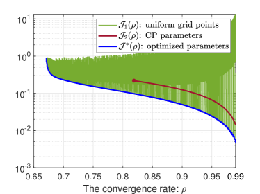
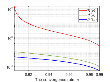
Figure 1: The rate-robustness trade-off for (38) when $\mu_{x}=\mu_{y}=1$, $\|K\|_{2}=10$, $d=30$ and $\delta_{x}=\delta_{y}=\delta=10$. The best achievable rate is $0.67$. The point indicated with a red $``*"$ in fig. 1 is the particular choice of CP parameters given in [8, Eq.(49)]. fig. 1 illustrates that employing the SAPD parameters obtained through minimizing $\bar{\mathcal{R}}$, an upper bound on $\mathcal{J}$ defined in section 3.2, one can closely track the efficient frontier $\mathcal{J}^{*}$. The best certifiable rate is $0.9049$.

We numerically illustrate the fundamental rate-robustness trade-off in fig. 1 for (38) through plotting 3 curves: $\mathcal{J}_{1}$, $\mathcal{J}_{2}$ and $\mathcal{J}^{*}$. For $\mathcal{J}_{1}$, we uniformly grid the parameter space $(\tau,\sigma,\theta)\in[0,0.5]\times[0,0.5]\times[0,2]$ using $500\times 500\times 200$ points; then, for each grid point, we compute the corresponding $(\rho_{\text{true}},\mathcal{J})$ values and plot it. For $\mathcal{J}_{2}$, we employ the step sizes suggested in [8, Algorithm 5] for the CP method and plot $(\rho_{\text{true}},\mathcal{J})$ (see section C.1) . For $\mathcal{J}^{*}$, defining $\mathcal{J}^{*}(\rho)\triangleq\min_{\tau,\sigma,\theta\geq 0}\{\mathcal{J}:\rho_{\text{true}}=\rho\}$, we plot $(\rho,\mathcal{J}^{*}(\rho))$ which illustrates the best robustness that can be achieved for a given rate. In the $\mathcal{J}_{1}$ plot, there are vertical lines as there exist many points in the grid sharing the same rate while they have very different robustness values. As seen in fig. 1, for great majority of parameter choice from the uniform grid, the corresponding robustness is very poor, i.e., very high $\mathcal{J}$ value. As a consequence, we infer that it is necessary to control the robustness through properly tuning the algorithm parameters. The $\mathcal{J}_{2}$ plot demonstrates that for a fixed rate CP parameter choice ensures relatively lower $\mathcal{J}$ values compared to the majority of points in the uniform grid; but, $\mathcal{J}_{2}$ is still far away from the efficient frontier $\mathcal{J}^{*}$. As indicated in $\mathcal{J}_{2}$ plot, the best convergence rate CP parameters can achieve is only around $0.83$, while the best rate achieved among the uniform grid is $0.67$.

While the parameter optimization problem to compute $\mathcal{J}^{*}(\rho)$ for a given convergence rate $\rho\in(0,1)$ can be done for (1) corresponding to (38), this is not a trivial task for a more general coupling function $\Phi$; therefore, we provide an alternative model to achieve a similar trade-off result between an upper bound on $\mathcal{J}$ and a bound on the convergence rate in Theorem 3.

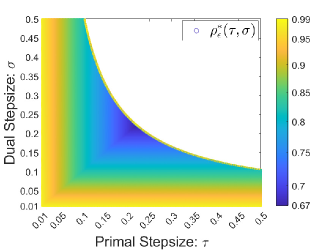
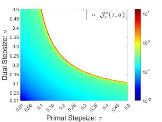
Figure 2: The effect of the step sizes on rate and robustness of SAPD running on (38) when $\mu_{x}=\mu_{y}=1$, $\|K\|_{2}=10$, $d=30$ and $\delta_{x}=\delta_{y}=\delta=10$. The best achievable rate is $0.67$.

Next, we analyze how primal-dual step sizes, $\tau$ and $\sigma$, affect the convergence rate and the robustness level. For any given $\epsilon\in(0,1)$, we define

$$\rho_{\epsilon}^{*}(\tau,\sigma)\triangleq\min_{{\theta}\geq 0}\{\rho_{\text{true}}:\rho_{\text{true}}{\leq}1-\epsilon\},\quad\mathcal{J}^{*}_{\epsilon}(\tau,\sigma)\triangleq\min_{\theta\geq 0}\{\mathcal{J}:\rho_{\text{true}}{\leq}1-\epsilon\}.$$

We consider the same experiment described in the caption of Figure 1, setting x-axis as $\tau$, and y-axis as $\sigma$, we plot $\rho_{\epsilon}^{*}(\tau,\sigma)$ in fig. 2 and $\mathcal{J}^{*}_{\epsilon}$ in fig. 2, for $\epsilon=0.01$. We observe that except for the boundary points, simultaneously increasing $\tau$ and $\sigma$ leads to a faster convergence rate at the expense of a decrease in robustness level – as one approaches the boundary, there is a significant increase in both convergence rate and $\mathcal{J}$ values. These results illustrate the fundamental trade-offs between the convergence rate and robustness for SAPD.

3.2 An Upper Bound for the Robustness Measure $\mathcal{J}$

$\mathcal{J}$ is hard to compute in general; to alleviate this issue, we can alternatively minimize an upper bound on $\mathcal{J}$ to control the robustness level. We start with a proposition that provides an upper bound on the robustness measure $\mathcal{J}$.

Theorem 3.

Suppose Assumptions 1, and 2 hold, and $\{x_{k},y_{k}\}_{k\geq 0}$ are generated by SAPD stated in Algorithm 1, the parameters $\{\tau,\sigma,\theta\}$ satisfy the conditions in Theorem 1 for some $\alpha\in[0,\tfrac{1}{\sigma})$ and $\rho\in(0,1)$.

Then, for $\delta\triangleq\min\{\delta_{x},\delta_{y}\}$ and $\Xi_{\tau,\sigma,\theta}$ as in Theorem 1, we have

$$\mathcal{J}=\limsup_{N\rightarrow\infty}\mathcal{J}_{N}\leq\frac{2\rho}{(1-{\rho})\delta^{2}}\cdot\max\Big{\{}\tau,\frac{\sigma}{1-\alpha\sigma}\Big{\}}\cdot\Xi_{\tau,\sigma,\theta}.$$ (45)

Proof.

Let $C_{\tau,\sigma}\triangleq\min\{{\frac{1}{2\tau},\frac{1}{2\sigma}(1-\alpha\sigma)}\}$. Then, from Theorem 1, we have that

$$C_{\tau,\sigma}\delta^{2}\mathcal{J}_{N}\leq\mathbb{E}\left[C_{\tau,\sigma}(\|x_{N}-x^{*}\|^{2}+\|y_{N}-y^{*}\|^{2})\right]\leq\rho^{N}D_{\tau,\sigma}+\frac{\rho}{1-\rho}~{}{\Xi}_{\tau,\sigma,\theta},$$

which implies (45) since $\rho^{N}D_{\tau,\sigma}\to 0$ as $N\to\infty$. ∎

This upper bound is theoretically correct only for parameters satisfying our step size conditions in eq. 5, which are only sufficient for ensuring a linear rate; but, they may not be necessary.

Next we investigate the trade-off between the convergence rate bound implied by the matrix inequality in eq. 5 and the robustness upper bound provided in Theorem 3.

Lemma 7.

Given $\rho\in(0,1)$, let $(t_{\rho},s_{\rho},\theta_{\rho},\alpha_{\rho})$ be an element of $\mathcal{P}_{\rho}$, where

$$\mathcal{P}_{\rho}\triangleq\{(t,s,\theta,\alpha):\ t,s,\theta,\alpha\geq 0,~{}\alpha\leq s,~{}G_{\rho}(t,s,\theta,\alpha)\succeq 0\}\ \hbox{and}$$

$$G_{\rho}(t,s,\theta,\alpha)\triangleq\begin{pmatrix}(1-\frac{1}{\rho})t+\mu_{x}&0&0&0&0\\ 0&(1-\frac{1}{\rho})s+\mu_{y}&(\frac{\theta}{\rho}-1)L_{yx}&(\frac{\theta}{\rho}-1)L_{yy}&0\\ 0&(\frac{\theta}{\rho}-1)L_{yx}&t-L_{xx}&0&-\frac{\theta}{\rho}L_{yx}\\ 0&(\frac{\theta}{\rho}-1)L_{yy}&0&s-\alpha&-\frac{\theta}{\rho}L_{yy}\\ 0&0&-\frac{\theta}{\rho}L_{yx}&-\frac{\theta}{\rho}L_{yy}&\frac{\alpha}{\rho}\end{pmatrix}.$$

Then the bias term, i.e., $\rho^{N}D_{\tau,\sigma}$ defined in (6), converges to $0$ with rate $\rho$ for SAPD employing $\tau=1/t_{\rho}$, $\sigma=1/s_{\rho}$ and $\theta=\theta_{\rho}$ . If $\mathcal{P}_{\rho}=\emptyset$, then (5) does not have a solution for the given $\rho$ value.

Proof.

This result immediately follows from Theorem 1. ∎

With the help of Lemma 7, one can do a binary search on $(0,1)$ interval to compute the best rate $\rho^{*}$ we can justify using the matrix inequality in (5), i.e., $\rho^{*}\triangleq\min_{\rho\geq 0}\{\rho:\mathcal{P}_{\rho}\neq\emptyset\}$. For any $\rho\in(0,1)$, checking whether $\mathcal{P}_{\rho}$ is nonempty or not requires solving a 4-dimensional SDP.

Next, we numerically illustrate that the explicit upper bound we derived in Theorem 3 provides a reasonable approximation to the actual robustness measure $\mathcal{J}$. For this purpose, we consider the same example from Section 3.1 where $\mathcal{J}$ can be explicitly computed, and compare $\mathcal{J}$ to its upper bound given in (45). In (38), we take $\mu_{x}=\mu_{y}=1$, where we generate the symmetric matrix $K\in\mathbb{R}^{d\times d}$ randomly with $\|K\|_{2}=10$ and $d=30$. We assume the noise model given in (39) and (40) with $\delta_{x}=\delta_{y}=10$. Consequently, we have $L_{xx}=L_{yy}=0$, $L_{yx}=10$. Employing the particular parameter choice in corollary 1, i.e., setting $\beta=1$, $\overline{\theta}_{2}=0$ and $c=1$, we can certify that SAPD converges with rate $\rho\approx 0.9049$ using $\tau$ and $\sigma$ as in (25) and $\theta=\rho$. We have found out that $\rho^{*}$ obtained using the binary search for this example was also equal to $0.9049$, i.e., our special solution in Corollary 1 leads to the optimal rate bound $\rho^{*}$.

For any $\rho\in[\rho^{*},1)$, we can optimize SAPD parameters minimizing the bound for robustness in (45) while ensuring that the bias term converges linearly with rate not worse than $\rho$, i.e.,

$${\color[rgb]{0,0,0}\mathcal{R}(\rho)}\triangleq \min_{\tau,\sigma,\theta,\alpha\geq 0}\left\{\frac{2\rho}{1-\rho}\cdot\max\Big{\{}\tau,\frac{\sigma}{(1-\alpha\sigma)}\Big{\}}\cdot\Xi_{\tau,\sigma,\theta}{\color[rgb]{0,0,0}/\delta^{2}}~{}:~{}\eqref{eq: general SAPD LMI_R1}{\color[rgb]{0,0,0}\text{ holds for }(\tau,\sigma,\theta,\rho,\alpha)}\right\}.$$ (46)

To be able to solve (46), we do not need to know $\delta_{x}$ or $\delta_{y}$. (46) is non-convex; however, it has some structure. In the next lemma, we provide a simpler optimization problem exploiting this structure.

Lemma 8.

Given $\rho\in(0,1)$ and $\tau>0$, let $S_{\rho}(\tau)\triangleq\{(\sigma,\theta,\alpha):\lx@cref{creftype~refnum}{eq: general SAPD LMI_R1}\text{ holds for }(\tau,\sigma,\theta,\rho,\alpha)\}$. Suppose $\cup_{\tau>0}S_{\rho}(\tau)\neq\emptyset$. Then, $\frac{1-\rho}{\mu_{x}\rho}=\min\{\tau:\ S_{\rho}(\tau)\neq\emptyset\}$. Moreover, for any $\tau_{1}\geq\tau_{2}\geq\frac{1-\rho}{\mu_{x}\rho}$, we have $S_{\rho}(\tau_{1})\subset S_{\rho}(\tau_{2})$. Finally, $\mathcal{R}(\rho)$ defined in eq. 46 can also be computed as

$${\color[rgb]{0,0,0}\mathcal{R}(\rho)=}\min_{\sigma,\theta,\alpha\geq 0}\Big{\{}\frac{2\rho}{1-\rho}\cdot\max\Big{\{}\tau,\frac{\sigma}{(1-\alpha\sigma)}\Big{\}}\cdot\Xi_{\tau,\sigma,\theta}{\color[rgb]{0,0,0}/\delta^{2}}~{}:~{}\tau=\frac{1-\rho}{\mu_{x}\rho},\quad\lx@cref{creftype~refnum}{eq: general SAPD LMI_R1}{\color[rgb]{0,0,0}\text{ holds}}\Big{\}}.$$ (47)

Proof.

Since $\cup_{\tau>0}S_{\rho}(\tau)\neq\emptyset$, there exists $(\tau,\sigma,\theta,\rho,\alpha)$ satisfying eq. 5; thus, $\tfrac{1}{\tau}(1-\tfrac{1}{\rho})+\mu_{x}\geq 0$, i.e., $\tau\geq\bar{\tau}\triangleq\frac{1-\rho}{\mu_{x}\rho}$. Say $\tau\geq\bar{\tau}$, then we have $\tfrac{1}{\bar{\tau}}-L_{xx}\geq\tfrac{1}{\tau}-L_{xx}$, which implies that $(\sigma,\theta,\alpha)\in S_{\rho}(\bar{\tau})$. Therefore, we can conclude that $\frac{1-\rho}{\mu_{x}\rho}=\min\{\tau:\ S_{\rho}(\tau)\neq\emptyset\}$ because eq. 5 requires that $\tau\geq\bar{\tau}$.

Suppose $(\sigma,\theta,\alpha)\in S_{\rho}(\tau_{1})$ for some $\tau_{1}>0$. The same arguments also show that for any $\tau_{2}\in[\frac{1-\rho}{\mu_{x}\rho},\tau_{1}]$, we have $(\sigma,\theta,\alpha)\in S_{\rho}(\tau_{2})$; hence, $S_{\rho}(\tau_{1})\subset S_{\rho}(\tau_{2})$. Furthermore, the objective in eq. 46 is strictly increasing in $\tau$; thus, the optimal values of eq. 46 and eq. 47 are equal. ∎

For any $\rho\in(0,1]$, we consider two necessary conditions for eq. 5: i) $\tau\geq\frac{1-\rho}{\mu_{x}\rho}$, ii) $\begin{pmatrix}\mu_{y}&\big{(}\tfrac{\theta}{\rho}-1\big{)}L_{yx}\\ \big{(}\tfrac{\theta}{\rho}-1\big{)}L_{yx}&\tfrac{1}{\tau}-L_{xx}\end{pmatrix}\succeq 0$, which further implies $(\tfrac{\theta}{\rho}-1)^{2}L_{yx}^{2}\leq\mu_{y}(\frac{1}{\tau}-L_{xx})$. Thus, for fixed $\rho$, any solution to eq. 5 satisfies $\theta\leq\bar{\theta}_{\rho}$, which is defined in (48). Indeed, either $\theta\in[0,\rho]$, or when $\theta\geq\rho$, the necessary conditions imply that

$$\theta\leq\rho\Bigg{(}1+\frac{\sqrt{\mu_{y}(\frac{1}{\tau}-L_{xx})}}{L_{yx}}\Bigg{)}\leq\rho\Bigg{(}1+\frac{\sqrt{\mu_{y}(\frac{\mu_{x}\rho}{1-\rho}-L_{xx})}}{L_{yx}}\Bigg{)}{\color[rgb]{0,0,0}\triangleq\overline{\theta}_{\rho}}.\vspace*{-1mm}$$ (48)

Next, we discuss how an upper bound on $\mathcal{J}$ can be computed efficiently through bisection over the rate parameter $\rho$ and a grid search on $\theta$.

Definition 1.

For $\rho\in(0,1)$, let $\mathcal{C}_{\rho}\triangleq\{c\in(0,1):\ \mathcal{P}_{\rho}\cap L_{c}\neq\emptyset\}$, where $\mathcal{P}_{\rho}$ is as in Lemma 7 and $L_{c}\triangleq\{(t,s,\theta,\alpha)\in\mathbb{R}^{4}_{+}:\alpha=cs\}$. The definition implies that $\mathcal{C}_{\rho}\neq\emptyset$ for all $\rho\in[\rho^{*},1)$.

Remark 7.

For any $\rho\in[\rho^{*},1)$, $\mathcal{C}_{\rho}\neq\emptyset$ is a convex set; hence, $\mathcal{C}_{\rho}\subset[0,1]$ is an interval. Thus, $\bar{c}_{\rho}\triangleq\sup\mathcal{C}_{\rho}$ and $\stackunder[1.2pt]{$c$}{\rule{3.44444pt}{0.32289pt}}_{\rho}\triangleq\inf\mathcal{C}_{\rho}$ can be computed via bisection. Each bisection iteration is a $3$-dimensional SDP checking the feasibility of $\{(t,s,\theta)\in\mathbb{R}^{3}_{+}:G_{\rho}(t,s,\theta,cs)\succeq\mathbf{0}\}$ for a given $c\in(0,1)$.

Lemma 9.

Given $\rho\in[\rho^{*},1)$ and $c\in\mathcal{C}_{\rho}$, let $\stackunder[1.2pt]{$\theta$}{\rule{3.44444pt}{0.32289pt}}_{c,\rho}\triangleq\inf\Theta_{c,\rho}$ and $\overline{\theta}_{c,\rho}\triangleq\sup\Theta_{c,\rho}$, where $\Theta_{c,\rho}\triangleq\{\theta:\ \exists(s,\theta)\in S_{c,\rho}\}$ and $S_{c,\rho}\triangleq\{(s,\theta):\ \exists(t,s,\theta,\alpha)\in\mathcal{P}_{\rho}\mbox{ s.t. }t=\frac{\mu_{x}\rho}{1-\rho},~{}\alpha=cs\}$. For fixed $K_{\theta}\in\mathbb{Z}_{+}$, let $\{\theta_{k}\}_{k=1}^{K_{\theta}}\subset[\stackunder[1.2pt]{$\theta$}{\rule{3.44444pt}{0.32289pt}}_{c,\rho},\overline{\theta}_{c,\rho}]\subset[0,\bar{\theta}_{\rho}]$ be an arbitrary set of grid points such that $\theta_{1}=\stackunder[1.2pt]{$\theta$}{\rule{3.44444pt}{0.32289pt}}_{c,\rho}$ and $\theta_{K_{\theta}}=\overline{\theta}_{c,\rho}$. Define $\bar{\mathcal{R}}_{c}(\rho)\triangleq\min_{k=1,\ldots K_{\theta}}\bar{\mathcal{R}}_{c}(\rho,\theta_{k})$, where

$$\bar{\mathcal{R}}_{c}(\rho,\theta)\triangleq\min_{\sigma\geq 0}\left\{\max\Big{\{}\frac{2}{\mu_{x}},~{}\frac{2\rho\sigma}{(1-c)(1-\rho)}\Big{\}}\cdot\Xi_{\tau,\sigma,\theta}/\delta^{2}:~{}\tau=\frac{1-\rho}{\mu_{x}\rho},~{}\alpha=\frac{c}{\sigma},~{}\lx@cref{creftype~refnum}{eq: general SAPD LMI_R1}{\color[rgb]{0,0,0}\text{ holds}}\right\}.$$ (49)

Then, $\bar{\mathcal{R}}_{c}(\rho)\geq\mathcal{R}(\rho)$. Furthermore, for any fixed $\rho\in[\rho^{*},1)$, $c\in\mathcal{C}_{\rho}$ and $\theta\in[\stackunder[1.2pt]{$\theta$}{\rule{3.44444pt}{0.32289pt}}_{c,\rho},\overline{\theta}_{c,\rho}]$, $\sigma_{c}(\rho,\theta)\triangleq 1/\max\{s:(s,\theta)\in S_{c,\rho}\}$ is the unique optimal solution to (49).

Proof.

Given $\rho\in[\rho^{*},1)$ and $c\in\mathcal{C}_{\rho}$, since we fix $\theta$ and $\alpha=c/\sigma$ while deriving eq. 49, we immediately get $\bar{\mathcal{R}}_{c}(\rho)\geq\mathcal{R}(\rho)$ due to Lemma 8. Lastly, after fixing $\rho\in[\rho^{*},1)$, $c\in\mathcal{C}_{\rho}$ and $\theta\in[\stackunder[1.2pt]{$\theta$}{\rule{3.44444pt}{0.32289pt}}_{c,\rho},\overline{\theta}_{c,\rho}]$, the objective in eq. 49 is increasing in $\sigma>0$, and $\sigma\mapsto 1/\sigma=s$ is a bijection between the feasible region of (49) and $\{s:(s,\theta)\in S_{c,\rho}\}$. Therefore, the unique solution $\sigma_{c}(\rho,\theta)$ can be computed by solving a one-dimensional SDP, i.e., $\max\{s:(s,\theta)\in S_{c,\rho}\}$ for fixed $\rho$, $c$ and $\theta$. ∎

Given $K_{c},K_{\rho}\in\mathbb{Z}_{+}$, let $P\triangleq\{\rho_{k}\}_{k=1}^{K_{\rho}}\subset[\rho^{*},1]$ and $C_{\rho}\triangleq\{c_{k}\}_{k=1}^{K_{c}}\subset\mathcal{C}_{\rho}$ be the grid points. Finally, for $\rho\in P$, we define $\bar{\mathcal{R}}(\rho)\triangleq\min_{c\in C_{\rho}}\bar{\mathcal{R}}_{c}(\rho)$, where $\bar{\mathcal{R}}_{c}(\rho)$ can be computed based on Lemma 9 for any $c\in C_{\rho}$. Therefore, for any $\rho\in P$, computing $\bar{\mathcal{R}}(\rho)$ using Lemma 9 will yield $(\tau_{\rho},\sigma_{\rho},\theta_{\rho})$ achieving $\bar{\mathcal{R}}_{c}(\rho)$ for some $c\in C_{\rho}$ such that $\bar{\mathcal{R}}(\rho)=\bar{\mathcal{R}}_{c}(\rho)$. Thus, for the quadratic model assumed in section 3.1, we can compute the robustness measure, defined in (37), corresponding to $(\tau_{\rho},\sigma_{\rho},\theta_{\rho})$, which we call $\mathcal{J}(\rho)$. Recall that in Section 3.1, we defined $\mathcal{J}^{*}(\rho)\triangleq\min_{\tau,\sigma,\theta\geq 0}\{\mathcal{J}:\rho_{\text{true}}=\rho\}$. To numerically illustrate the rate vs robustness trade-off and also to demonstrate that we can control robustness through optimizing $\bar{\mathcal{R}}$, in fig. 1, we plot robustness measure $\mathcal{J}(\rho)$, corresponding to $(\tau_{\rho},\sigma_{\rho},\theta_{\rho})$ computed by minimizing its upper bound $\bar{\mathcal{R}}(\rho)$, against the convergence rate values $\rho\in P$ in the x-axis, and compare $\mathcal{J}(\rho)$ with $\mathcal{J}^{*}(\rho)$ and $\bar{\mathcal{R}}(\rho)$, where we set $K_{\rho}=K_{\theta}=100$ and $K_{c}=50$. In fig. 1, we observe that $\mathcal{J}(\rho)$ computed for SAPD parameters optimizing $\bar{\mathcal{R}}(\rho)$ closely tracks $\mathcal{J}^{*}(\rho)$. Therefore, we infer that minimizing the upper bound helps us optimize the robustness for the problem class used in these experiments.

4 Extensions

We now show that SAPD admits the optimal oracle complexity bound for the stochastic MCMC case, i.e., when $\mu_{x}=\mu_{y}=0$. This result can be viewed as a nontrivial extension of the deterministic complexity result in [18] to the stochastic gradient setting.

Remark 8.

Suppose $\mu_{x}=\mu_{y}=0$, and the parameters $\tau,\sigma>0$ and $\theta\in(0,1]$ satisfy (7). The first condition (7) implies that $\theta=1$.

Theorem 4.

Suppose $\mu_{x}=\mu_{y}=0$, Assumptions 1 and 2 hold. Assume that $\Omega_{x}\triangleq\sup_{x_{1},x_{2}\in\mathop{\bf dom}f}\|x_{1}-x_{2}\|<\infty$ and $\Omega_{y}\triangleq\sup_{y_{1},y_{2}\in\mathop{\bf dom}g}\|y_{1}-y_{2}\|<\infty$. For any $\epsilon>0$, suppose $\{\tau,\sigma,\theta\}$ are chosen such that

$$\tau=\min\Big{\{}\frac{1}{L_{yx}+L_{xx}},~{}{\color[rgb]{0,0,0}{\frac{{\color[rgb]{0,0,0}2}}{15}}\cdot\frac{\epsilon}{\delta_{x}^{2}}}\Big{\}},\quad\sigma=\min\Big{\{}\frac{1}{{\color[rgb]{0,0,0}L_{yx}+2L_{yy}}},~{}{\color[rgb]{0,0,0}\frac{1}{L_{xy}}},~{}{\color[rgb]{0,0,0}\frac{1}{{\color[rgb]{0,0,0}72}}}\cdot\frac{\epsilon}{\delta_{y}^{2}}\Big{\}},\quad\theta=1.$$ (50)

Then for the gap metric $\mathcal{G}(\cdot,\cdot)$, defined in (2), $\mathcal{G}(\bar{x}_{N},\bar{y}_{N})\leq\epsilon$ for all $N\geq N_{\epsilon}$ such that

$${\color[rgb]{0,0,0}N_{\epsilon}}=\mathcal{O}\Big{(}\frac{(L_{yx}+L_{xx}){\Omega_{x}^{2}}+{\color[rgb]{0,0,0}\max\{L_{yx}+L_{yy},~{}L_{xy}\}}{\Omega_{y}^{2}}}{\epsilon}+\frac{\delta_{x}^{2}{\Omega_{x}^{2}}+\delta_{y}^{2}{\Omega_{y}^{2}}}{\epsilon^{2}}\Big{)}.$$

Proof.

Since $\mu_{x}=\mu_{y}=0$, the first condition in (7) trivially holds for $(\tau,\sigma,\theta)$ as in (50). Furthermore, (50) implies that $\frac{1}{\tau}\geq L_{yx}+L_{xx}$ and $\frac{1}{\sigma}\geq L_{yx}+2L_{yy}$; therefore, $(\tau,\sigma,\theta)$ in (50) with $\pi_{1}=\pi_{2}=1$ satisfy the conditions in Lemma 6. Thus, $(\tau,\sigma,\theta)$ with $\alpha=L_{yx}+L_{yy}$ solves (7).

The analysis in the proof of Theorem 1 until the end of (22) is valid for our choice of parameters in (50). To get a bound for the expected gap, we next analyze $\bar{P}\triangleq\sup\{\sum_{k=0}^{N-1}P_{k}(x,y):(x,y)\in\mathop{\bf dom}f\times\mathop{\bf dom}g\}$. For some arbitrary $\eta_{x}>0$, define $\{\tilde{x}_{k}\}$ sequence as follows: $\tilde{x}_{0}\triangleq x_{0}$, and $\tilde{x}_{k+1}\triangleq\operatorname*{\textbf{argmin}}_{x^{\prime}\in\mathop{\bf dom}f}-\langle\Delta^{x}_{k},x^{\prime}\rangle+\frac{{\color[rgb]{0,0,0}\eta_{x}}}{2}\|x^{\prime}-\tilde{x}_{k}\|^{2}$, for $k\geq 0$, where $\Delta_{k}^{x}$ is defined as in Lemma 2. Then, from [32, Lemma 2.1], for all $x\in\mathop{\bf dom}f$ we get

$$\sum_{k=0}^{N-1}\langle\Delta^{x}_{k},x-\tilde{x}_{k}\rangle\leq\sum_{k=0}^{N-1}\frac{\eta_{x}}{2}\|x-\tilde{x}_{k}\|^{2}-\frac{\eta_{x}}{2}\|x-\tilde{x}_{k+1}\|^{2}+\frac{1}{2\eta_{x}}\|\Delta^{x}_{k}\|^{2}\leq{\frac{\eta_{x}}{2}}{\color[rgb]{0,0,0}\|x-x_{0}\|^{2}}+{\frac{1}{2\eta_{x}}}\sum_{k=0}^{N-1}\|\Delta^{x}_{k}\|^{2};$$ (51)

hence, using $\hat{x}_{k+1}$ defined in Lemma 2, we get

$$\mathbb{E}\Big{[}\sup_{x\in\mathop{\bf dom}f}\Big{\{}\sum_{k=0}^{N-1}-\langle\Delta^{x}_{k},\hat{x}_{k+1}-x\rangle\Big{\}}\Big{]}\leq\sum_{k=0}^{N-1}\mathbb{E}\Big{[}\langle\Delta^{x}_{k},\tilde{x}_{k}-{\hat{x}_{k+1}}\rangle+\frac{1}{2{\color[rgb]{0,0,0}\eta_{x}}}\|\Delta^{x}_{k}\|^{2}\Big{]}+\frac{{\color[rgb]{0,0,0}\eta_{x}}}{2}\Omega_{x}^{2}.$$ (52)

Similarly, for arbitrary $\eta_{y}>0$, we construct two auxiliary sequences: let $\tilde{y}_{0}^{+}=\tilde{y}_{0}^{-}=y_{0}$, and we define $\tilde{y}^{+}_{k+1}\triangleq\operatorname*{\textbf{argmin}}_{y^{\prime}\in\mathop{\bf dom}g}\langle\Delta^{y}_{k},y^{\prime}\rangle+\frac{{\color[rgb]{0,0,0}\eta_{y}}}{2}\|y^{\prime}-\tilde{y}^{+}_{k}\|^{2}$, and $\tilde{y}^{-}_{k+1}\triangleq\operatorname*{\textbf{argmin}}_{y^{\prime}\in\mathop{\bf dom}g}-\langle\Delta^{y}_{k},y^{\prime}\rangle+\frac{{\color[rgb]{0,0,0}\eta_{y}}}{2}\|y^{\prime}-\tilde{y}^{-}_{k}\|^{2}$, for $k\geq 0$. Thus, as in as in (51), it follows from [32, Lemma 2.1] that for all $y\in\mathop{\bf dom}g$, we get

$$\sum_{k=0}^{N-1}2\langle\Delta^{y}_{k},\tilde{y}_{k}^{+}-y\rangle-\langle\Delta^{y}_{k-1},\tilde{y}_{k-1}^{-}-y\rangle\leq\frac{3\eta_{y}}{2}{\color[rgb]{0,0,0}\|y-y_{0}\|^{2}}+\frac{1}{2\eta_{y}}\sum_{k=0}^{N-1}2\|\Delta^{y}_{k}\|^{2}+\|\Delta^{y}_{k-1}\|^{2};$$

hence, using $\hat{y}_{k+1}$ and $\hat{\hat{y}}_{k+1}$ defined in Lemma 2, we get

$$\mathbb{E}\Big{[}\sup_{y\in\mathop{\bf dom}g}\Big{\{}\sum_{k=0}^{N-1}2\langle\Delta^{y}_{k},{\hat{y}_{k+1}}-y\rangle-\langle\Delta^{y}_{k-1},{\hat{\hat{y}}_{k+1}}-y\rangle\Big{\}}\Big{]}$$

$$\leq \sum_{k=0}^{N-1}\mathbb{E}\Big{[}2\langle\Delta^{y}_{k},{\hat{y}_{k+1}}-\tilde{y}_{k}^{+}\rangle-\langle\Delta^{y}_{k-1},{\hat{\hat{y}}_{k+1}}-\tilde{y}_{k-1}^{-}\rangle+\frac{1}{2{\eta_{y}}}\Big{(}2\|\Delta^{y}_{k}\|^{2}+\|\Delta^{y}_{k-1}\|^{2}\Big{)}\Big{]}+\frac{{\color[rgb]{0,0,0}3\eta_{y}}}{2}\Omega_{y}^{2}.$$

Thus, combining this bound with (52) we get $\mathbb{E}[\bar{P}]\leq N(\frac{1}{2}\frac{\delta_{x}^{2}}{\eta_{x}}+\frac{3}{2}\frac{\delta_{y}^{2}}{\eta_{y}})+\frac{\eta_{x}}{2}\Omega_{x}^{2}+\frac{3\eta_{y}}{2}\Omega_{y}^{2}$, where we used $\mathbb{E}[\langle\Delta^{x}_{k},\tilde{x}_{k}-{\hat{x}_{k+1}}\rangle]=\mathbb{E}[\langle\Delta^{y}_{k},{\hat{y}_{k+1}}-\tilde{y}_{k}^{+}\rangle]=\mathbb{E}[\langle\Delta^{y}_{k-1},{\hat{\hat{y}}_{k+1}}-\tilde{y}_{k-1}^{-}\rangle]=0$ for $k\geq 0$. Therefore, setting $\eta_{x}=1/\tau$ and $\eta_{y}=1/\sigma$ and using the fact that $\theta=1$ implies $K_{N}(\theta)=N$, it follows from (19), (20) and (22) that

$$\mathbb{E}[ \sup_{(x,y)\in\mathcal{X}\times\mathcal{Y}}\{\mathcal{L}(\bar{x}_{N},y)-\mathcal{L}(x,\bar{y}_{N})\}]$$ (53)

$$\leq\frac{1}{N}\Big{(}\frac{1}{\tau}{\Omega_{x}^{2}}+\frac{2}{\sigma}{\Omega_{y}^{2}}\Big{)}+{\tau(1+{\color[rgb]{0,0,0}2}\Xi^{x}_{\tau,\sigma,\theta})\frac{\delta_{x}^{2}}{2}+\sigma(3+{\color[rgb]{0,0,0}2}\Xi^{y}_{\tau,\sigma,\theta})\frac{\delta_{y}^{2}}{2}}\leq\frac{1}{N}\Big{(}\frac{1}{\tau}{\Omega_{x}^{2}}+\frac{2}{\sigma}{\Omega_{y}^{2}}\Big{)}+{\frac{5\tau\delta_{x}^{2}}{2}}+{\color[rgb]{0,0,0}24\sigma\delta_{y}^{2}},$$

where for the last inequality we first substitute $\Xi^{x}_{\tau,\sigma,\theta}$ and $\Xi^{y}_{\tau,\sigma,\theta}$ defined in Theorem 1, and then use $\tau L_{yx}\leq 1$, $\sigma\max\{L_{yx},L_{xy}\}\leq{\color[rgb]{0,0,0}1}$ and $\sigma L_{yy}\leq\frac{1}{2}$ due to eq. 50. For any $\epsilon>0$, requiring

$$\frac{1}{N}\Big{(}\frac{1}{\tau}{\Omega_{x}^{2}}+\frac{2}{\sigma}{\Omega_{y}^{2}}\Big{)}{\leq}\frac{\epsilon}{3},\quad\frac{5\tau\delta_{x}^{2}}{{\color[rgb]{0,0,0}2}}\leq\frac{\epsilon}{3},\quad{\color[rgb]{0,0,0}24\sigma\delta_{y}^{2}}\leq\frac{\epsilon}{3},$$ (54)

implies that (53) can be bounded by $\epsilon$. Our parameter choice in (50) implies that the second and the third inequalities in (54) trivially hold. It suffices to choose $N$ large enough depending on given $\epsilon$ so that (54) holds, i.e., $N\geq\frac{3}{\epsilon}(\frac{1}{\tau}{\Omega_{x}^{2}}+\frac{2}{\sigma}{\Omega_{y}^{2}})$. From (50) we have $\frac{1}{\tau}\leq L_{yx}+L_{xx}+{\frac{15}{{\color[rgb]{0,0,0}2}}\frac{\delta_{x}^{2}}{\epsilon}}$ and $\frac{1}{\sigma}\leq{\color[rgb]{0,0,0}\max\{L_{yx}+2L_{yy},~{}L_{xy}\}}+{\color[rgb]{0,0,0}72}\frac{\delta_{y}^{2}}{\epsilon}$; thus, $\mathcal{G}(\bar{x}_{N},\bar{y}_{N})\leq\epsilon$ holds for all $N\geq N_{\epsilon}$. ∎

4.1 Robustness measure for MCMC setting

In MCMC setting, based on the gap result in Theorem 4, one can adopt $\tilde{J}\triangleq\limsup_{N\to\infty}\mathbb{E}[\sup\{\mathcal{L}(\bar{x}_{N},y)-\mathcal{L}(x,\bar{y}_{N}):(x,y)\in\mathcal{X}\times\mathcal{Y}\}]$ as the corresponding robustness metric –this definition would be parallel to the definition in [2], where the authors consider first-order stochastic algorithms for smooth strongly convex minimization $f^{*}=\min_{x}f(x)$ and defined the robustness as $\limsup_{N\to\infty}\mathbb{E}[f(x_{N})-f^{*}]$.

Alternatively, one can extend the ideas of SCSC setting to MCMC setting in the following way based on Tikhonov regularization. Assume $\mu_{x}=\mu_{y}=0$ and consider the MCMC saddle point problem $\min_{x}\max_{y}\mathcal{L}(x,y)$. Given a regularization parameter $\mu>0$, let $\mathcal{J}_{\mu}$ be the robustness of the SAPD iterate sequence generated when SAPD is implemented on the following regularized problem:

$$\min_{x\in\mathcal{X}}\max_{y\in\mathcal{Y}}\mathcal{L}_{\mu}(x,y)\triangleq\mathcal{L}(x,y)+\frac{\mu}{2}\|x\|^{2}-\frac{\mu}{2}\|y\|^{2},$$ (55)

where $\mathcal{L}_{\mu}$ is $\mu$-convex in $x$ and $\mu$-concave in $y$. Using the results in [14], under some technical conditions on $\mathcal{L}$, e.g., $\Phi$ is smooth convex-concave and $f,g$ are indicator functions of some polyhedra, one can show that there exists $\bar{\mu}>0$ and $({x}^{*},{y}^{*})\in\mathcal{X}\times\mathcal{Y}$ such that $({x}^{*},{y}^{*})$ is the unique saddle point of $\mathcal{L}_{\mu}(\cdot,\cdot)$ for all $\mu\in(0,\bar{\mu}]$; moreover, $({x}^{*},{y}^{*})=\operatorname*{\textbf{argmin}}\{\|x\|^{2}+\|y\|^{2}:\ (x,y)\in\mathcal{Z}^{*}\}$ where $\mathcal{Z}^{*}\subset\mathcal{X}\times\mathcal{Y}$ denotes the set of saddle points of the original MCMC problem $\min_{x}\max_{y}\mathcal{L}(x,y)$. Therefore, rather than directly solving the MCMC problem with SAPD using the parameters as stated in Theorem 4 and use the alternative robustness measure $\tilde{J}$ based on the expected gap defined above, one can instead solve the regularized SCSC problem in (55) for $\mu>0$ sufficiently small, which would generate a least-norm solution of the original MCMC problem, and directly use the originally defined robustness metric $\mathcal{J}_{\mu}={\limsup_{N\to\infty}\mathbb{E}[\|x_{N}-x^{*}\|^{2}/\delta_{x}^{2}+\|y_{N}-y^{*}\|/\delta_{y}^{2}]}$ corresponding to the SAPD iterate sequence generated while solving the SCSC problem in (55).

5 Numerical experiments

In this section, we compared SAPD against S-OGDA [13], SMD [32] and SMP [22] for solving (1) with synthetic and real-data.

5.1 Regularized Bilinear SP Problem with Synthetic Data

We first tested SAPD, S-OGDA and SMP on the regularized bilinear SP problem defined in (38). In this experiment, we set $\mu_{x}=\mu_{y}=1$, $\|K\|_{2}=10$, $d=30$ and $\delta_{x}=\delta_{y}=\delta=5$. Since SMD step size condition requires a bound on the stochastic gradients, SMD is implemented on (38) with additional $(x,y)\in X\times Y$ constraint where $X=\{x\in\mathcal{X}:\|x\|\leq\sqrt{d}\}$ and $Y=\{y\in\mathcal{Y}:\|y\|\leq\sqrt{d}\}$. Letting $x$-axis as the iteration counter, we plot the $50$ sample paths for each algorithm in fig. 3. The step sizes for S-OGDA, SMD and SMP are selected as in [13], [32] and [22], respectively. Specifically, except for SAPD, all algorithms use primal and dual step sizes that are set equal, and their value is a function of $L=\max\{\mu_{x},\mu_{y},L_{xy},L_{yx}\}$; indeed, S-OGDA uses $\frac{1}{8L}$, SMP uses $\frac{1}{\sqrt{3}L}$, and SMD uses $\frac{2}{\sqrt{5GN}}$, where $N$ denotes the total iteration budget for SMD, and $G>0$ is such that $\mathbb{E}[2\|\tilde{\nabla}\mathcal{L}(x,y;\omega^{x},\omega^{y})\|^{2}]\leq G$ uniformly for all $(x,y)\in X\times Y$. The step sizes for SAPD are determined by minimizing $\bar{\mathcal{R}}(\rho)$ for $\rho\in\{\rho_{1},\rho_{2}\}$, where $\rho_{1}=0.99$ and $\rho_{2}=0.995$. This process leads to $(\tau,\sigma,\theta)=(0.010,0.012,0.645)$ for $\text{SAPD}(\rho_{1})$, and to $(\tau,\sigma,\theta)=(0.005,0.008,0.174)$ for $\text{SAPD}(\rho_{2})$. In Figure 3, SAPD outperforms the others in both metrics, i.e., $\mathcal{D}$ and $\mathcal{G}$. Since $\rho_{1}<\rho_{2}$, SAPD with $\rho=\rho_{1}$ leads to a faster decay of the bias term than that with $\rho=\rho_{2}$. However, due to rate and robustness trade-off, the choice of $\rho=\rho_{2}$ is more robust to noise, leading to a smaller asymptotic variance of $\{z_{k}\}$ as expected.

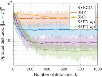
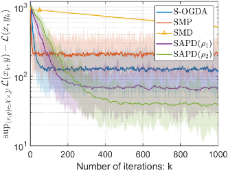
Figure 3: Comparison of SAPD against SOGDA, SMP and SMD on a synthetic toy problem using the distance (left) and gap (right) metrics. The rates of SAPD are $\rho_{1}=0.99$ and $\rho_{2}=0.995$.

5.2 Distributionally Robust Optimization with Real Data

Next, we consider $\ell_{2}$-regularized variant of the distributionally robust optimization problem from [29], i.e., (DRO): $\min_{{\color[rgb]{0,0,0}x\in\mathcal{S}}}\max_{{\color[rgb]{0,0,0}y}\in\mathcal{P}_{{\color[rgb]{0,0,0}r}}}\tfrac{{\color[rgb]{0,0,0}\mu_{x}}}{2}\|x\|^{2}+\sum_{i=1}^{n}{\color[rgb]{0,0,0}y_{i}}{\color[rgb]{0,0,0}\phi_{i}(x)}$ where ${\color[rgb]{0,0,0}\phi_{i}}:\mathbb{R}^{d}\to\mathbb{R}$ is a strongly convex smooth loss function corresponding to the $i$-th data point, $\mu_{x}>0$ is a regularization parameter, $\mathcal{S}\triangleq\{x\in\mathbb{R}^{d}:\ \|x\|^{2}\leq\mathcal{D}_{x}\}$ for some given model diameter $\mathcal{D}_{x}>0$ and $\mathcal{P}_{{\color[rgb]{0,0,0}r}}\triangleq\{y\in\mathbb{R}^{n}_{+}:~{}\mathbf{1}^{\top}y=1,~{}\|y-\mathbf{1}/n\|^{2}\leq\frac{r}{n^{2}}\}$ – here, $\mathbf{1}$ denotes the vector with all entries equal to one, and $\mathcal{P}_{r}$ is the uncertainty set around the uniform distribution $\mathbf{1}/n$ whose radius is determined by the parameter $r$. In the special case when $r=0$, the problem recovers the ERM problems arising in supervised learning from labeled data which assigns uniform weights $y_{i}=1/n$ to all data points. When $r>0$, the problem is to minimize a worst-case objective to be robust against uncertainty in the underlying data distribution. (DRO) has several advantages to construct confidence intervals for the parameters of predictive models in supervised learning, see [29]. This SP problem is affine in the dual variable $y$; therefore, it is not strongly convex with respect to $y$. However, we can approximate it, in a similar spirit to Nesterov’s smoothing technique in [34], with the following SCSC problem:

$${\color[rgb]{0,0,0}\min_{x\in\mathcal{S}}\max_{y\in\mathcal{P}_{r}}\mathcal{L}_{\mu_{y}}(x,y)\triangleq\tfrac{{\color[rgb]{0,0,0}\mu_{x}}}{2}\|x\|^{2}+\Phi(x,y)-\tfrac{{\mu_{y}}}{2}\|y\|^{2},}$$ (56)

where $\Phi(x,p)=\sum_{i=1}^{n}y_{i}\phi_{i}(x)$ for some properly chosen smoothing parameter $\mu_{y}>0$ –see remark 5. In our tests, we consider the binary logistic loss with an $l_{2}$ regularizer, i.e., $\phi_{i}(x)=\ln(1+\exp(-b_{i}{\color[rgb]{0,0,0}a_{i}}^{\top}x))$ and set $r=2\sqrt{n}$. We can then apply SAPD to the SCSC problem in (56) which admits the Lipschitz constants $L_{xy}=L_{yx}=\|A\|_{2}$, $L_{xx}=\max_{{\color[rgb]{0,0,0}i=1,\ldots,n}}\{\tfrac{1}{4}\|a_{i}\|_{2}^{2}$}, and $L_{yy}=0$, where $A\in\mathbb{R}^{n\times d}$ is the data matrix with rows $\{a_{i}\}_{i=1}^{n}$ and columns $\{A_{j}\}_{j=1}^{d}$. Since $\mathcal{D}_{y}\triangleq\sup_{y\in\mathcal{P}_{r}}\|y\|=1$, for any given $\epsilon>0$, we set $\mu_{y}=\frac{\epsilon}{2\mathcal{D}_{y}^{2}}$ according to remark 5.

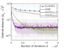
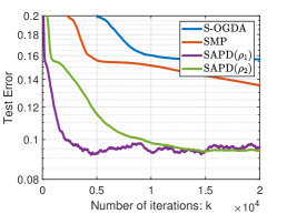
(a) Dry Bean: $\rho_{1}=0.9986$, $\rho_{2}=0.9997$.

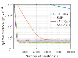
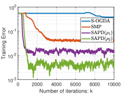
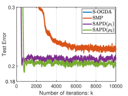
(b) Arcene: $\rho_{1}=0.989$, $\rho_{2}=0.992$.

Figure 4: Comparison of SAPD against S-OGDA [13] and SMP [22] on real-data sets.

We perform experiments on two data sets: 1) Dry Bean data set [23] with $d=16$, $n=9528$ with a test data set of $4083$ points; 2) Arcene data set [17] with $d=10,000$, $n=97$ and test size of $96$ points. In these experiments we set the regularization parameter $\mu_{x}$ through cross-validation. The source of noise in gradient computations is mini-batch sampling of data. For the Dry Bean data set, we set $\mu_{x}=0.01$, $\mu_{y}=10$ and use batch size $1$, and normalize each feature column $A_{j}\in\mathbb{R}^{n}$ using $A_{j}\leftarrow\frac{A_{j}-\min(A_{j})}{\max(A_{j})-\min(A_{j})}$, where both min and max are taken over the elements of $A_{j}$. For the Arcene data set, we set $\mu_{x}=0.02$ and $\mu_{y}=10$, and use batch size 10, and normalize the data matrix such that $A\leftarrow A/\min\{\sqrt{d},\sqrt{n}\}$. As described in Section 3.2, given a desired rate $\rho\geq\rho^{*}$, we compute $(\tau,\sigma,\theta)$ for SAPD that achieves $\bar{\mathcal{R}}(\rho)$. We plot SAPD statistics for two different rates to illustrate that our framework can trade-off rate and robustness in an effective manner. The other methods we tested set the primal and dual step sizes equal. Indeed, for S-OGDA [19, 13] the step size is $\frac{1}{8L}$, and for SMP [22], it is $\frac{1}{\sqrt{3}L}$, where $L=\max\{L_{xx}+\mu_{x},\mu_{y},L_{xy},L_{yx}\}$. In fig. 4, we plotted the optimization error using the distance metric $\mathcal{D}$, training and the test errors. We reported the results for 50 sample paths. Our results show that for both test and training errors, reported in terms of distances to the solution, SAPD achieves a good performance for both rate and robustness.

6 Future Work

In a follow-up paper [52], we have considered SARAH variance reduction [36] on weakly convex-strongly concave (WCSC) problems, and proposed an inexact proximal point method based on SAPD, which serves as a subroutine for inexactly solving SCSC sub-problems. We have implemented a variance reduction framework within SAPD, which not only improved the oracle complexity from $\mathcal{O}(\epsilon^{-4})$ to $\mathcal{O}(\epsilon^{-3})$; but, we have also improved the best condition number dependency from $\mathcal{O}(L\kappa^{3}/\epsilon^{3})$ to $\mathcal{O}(L\kappa^{2}/\epsilon^{3})$, where $\kappa\triangleq L/\mu_{y}$ with $L$ being the Lipschitz constant of $\nabla\Phi$ and $\mu_{y}$ being the strong concavity constant of $\mathcal{L}(x,\cdot)$ uniformly for all $x\in\mathop{\bf dom}f$. While incorporating SARAH within SAPD helps for WCSC problems, using the same variance reduction analysis for SAPD on SCSC problems does not help in improving the complexity results we established in Theorem 2. That being said, for the SCSC case, in a recent relevant paper, we have applied a bias reduction strategy called Richardson-Romberg extrapolation to SAPD [6] and in our experiments we have observed that this technique has not only created an improved bias performance but also exhibits an improved dependency to gradient noise variance. As a future work on the SCSC setting with noisy gradients, it would be interesting to design efficient variance/bias reduction techniques for SAPD. The method in [52] has two nested loops, another important future research direction involves establishing convergence guarantees for SAPD as a single-loop method when implemented for solving WCSC and weakly convex-merely-concave problems.

Appendix A Proofs of Lemmas

A.1 Auxiliary Results

Lemma 10.

Let $f$ be proper, closed and strongly convex with modulus $\mu>0$. Then for any $x,x^{\prime}\in\mathop{\bf dom}f$, and $c>0$, $\|\mathbf{prox}_{cf}(x)-\mathbf{prox}_{cf}(x^{\prime})\|\leq\frac{1}{1+c\mu}\|x-x^{\prime}\|.$

Because Lemma 10 is a simple extension of [3, Theorem 6.42] to the strongly convex scenario, we omit its proof.

A.2 Proof of Lemma 1

Fix $x\in\mathop{\bf dom}f$ and $y\in\mathop{\bf dom}g$. Invoking [18, Lemma 7.1] for the $y-$ and $x-$subproblems in Algorithm 1, and using the definitions of $\varepsilon^{x}_{k}$ and $\varepsilon^{y}_{k}$, we get

$$f(x_{k+1}) +\langle{{\nabla}_{x}\Phi(x_{k},y_{k+1})},~{}x_{k+1}-x\rangle$$ (57a)

$$\leq f(x)+\tfrac{1}{2\tau}(\|x-x_{k}\|^{2}-\|x-x_{k+1}\|^{2}-\|x_{k+1}-x_{k}\|^{2}){-\tfrac{\mu_{x}}{2}\|x-x_{k+1}\|^{2}}+{\varepsilon^{x}_{k}},$$

$$-g(y) +g(y_{k+1})$$ (57b)

$$\leq \langle s_{k},y_{k+1}-y\rangle+\tfrac{1}{2\sigma}\left[\|y-y_{k}\|^{2}-\|y-y_{k+1}\|^{2}-\|y_{k+1}-y_{k}\|^{2}\right]-\tfrac{\mu_{y}}{2}\|y-y_{k+1}\|^{2}{+\varepsilon^{y}_{k}}.$$

Since $y_{k+1}\in\mathop{\bf dom}g$, the inner product in (57a) can be lower bounded using convexity of $\Phi(\cdot,y_{k+1})$ in Assumption 1 as follows:

$$\langle\nabla_{x}\Phi(x_{k},y_{k+1}),x_{k+1}-x\rangle= \langle\nabla_{x}\Phi(x_{k},y_{k+1}),x_{k}-x\rangle+\langle\nabla_{x}\Phi(x_{k},y_{k+1}),x_{k+1}-x_{k}\rangle$$

$$\geq \Phi(x_{k},y_{k+1})-\Phi(x,y_{k+1})+\langle\nabla_{x}\Phi(x_{k},y_{k+1}),~{}x_{k+1}-x_{k}\rangle.$$

Using this inequality after adding $\Phi(x_{k+1},y_{k+1})$ to both sides of (57a), we get

$$\Phi(x_{k+1}, y_{k+1})+f(x_{k+1})$$ (58)

$$\leq \Phi(x,y_{k+1})+f(x)+\Phi(x_{k+1},y_{k+1})-\Phi(x_{k},y_{k+1})-\langle\nabla_{x}\Phi(x_{k},y_{k+1}),x_{k+1}-x_{k}\rangle$$

$$+\tfrac{1}{2\tau}\left[\|x-x_{k}\|^{2}-\|x-x_{k+1}\|^{2}-\|x_{k+1}-x_{k}\|^{2}\right]-\tfrac{\mu_{x}}{2}\|x-x_{k+1}\|^{2}+{\color[rgb]{0,0,0}\varepsilon^{x}_{k}}$$

$$\leq \Phi(x,y_{k+1})+f(x)+\frac{L_{xx}}{2}\|x_{k+1}-x_{k}\|^{2}$$

$$+\tfrac{1}{2\tau}\left[\|x-x_{k}\|^{2}-\|x-x_{k+1}\|^{2}-\|x_{k+1}-x_{k}\|^{2}\right]-\tfrac{\mu_{x}}{2}\|x-x_{k+1}\|^{2}+{\color[rgb]{0,0,0}\varepsilon^{x}_{k}},$$

where the last step follows from Assumption 1, i.e., $\nabla_{x}\Phi(\cdot,y_{k+1})$ is Lipschitz with constant $L_{xx}$. Rearranging the terms gives us

$$f( x_{k+1})-f(x)-\Phi(x,y_{k+1})\leq-\Phi(x_{k+1},y_{k+1})+\frac{L_{xx}}{2}\|x_{k+1}-x_{k}\|^{2}$$ (59)

$$+\frac{1}{{\color[rgb]{0,0,0}2}\tau}\left[\|x-x_{k}\|^{2}-\|x-x_{k+1}\|^{2}-\|x_{k+1}-x_{k}\|^{2}\right]-\frac{\mu_{x}}{2}\|x-x_{k+1}\|^{2}+{\color[rgb]{0,0,0}\varepsilon^{x}_{k}}.$$

Then, for $k\geq 0$, by summing (57b) and (59), we obtain

$$\mathcal{L}(x_{k+1},y)-\mathcal{L}(x,y_{k+1}) =f(x_{k+1})+\Phi(x_{k+1},y)-g(y)-f(x)-\Phi(x,y_{k+1})+g(y_{k+1})$$ (60)

$$\leq\Phi(x_{k+1},y)-\Phi(x_{k+1},y_{k+1})+\langle s_{k},y_{k+1}-y\rangle+\frac{L_{xx}}{2}\|x_{k+1}-x_{k}\|^{2}$$

$$\ +\frac{1}{{\color[rgb]{0,0,0}2}\sigma}\left[\|y-y_{k}\|^{2}-\|y-y_{k+1}\|^{2}-\|y_{k+1}-y_{k}\|^{2}\right]-\frac{\mu_{y}}{2}\|y-y_{k+1}\|^{2}+{\varepsilon_{k}^{y}}$$

$$\ +\frac{1}{{\color[rgb]{0,0,0}2}\tau}\left[\|x-x_{k}\|^{2}-\|x-x_{k+1}\|^{2}-\|x_{k+1}-x_{k}\|^{2}\right]-\frac{\mu_{x}}{2}\|x-x_{k+1}\|^{2}+{\varepsilon_{k}^{x}}.$$

From Assumption 1, the concavity of $\Phi(x,\cdot)$ for fixed $x\in\mathop{\bf dom}f\subset\mathcal{X}$ implies

$$\Phi(x_{k+1},y)- \Phi(x_{k+1},y_{k+1})+\langle s_{k},y_{k+1}-y\rangle$$

$$\leq \langle\nabla_{y}\Phi(x_{k+1},y_{k+1}),y-y_{k+1}\rangle+\langle\nabla_{y}\Phi(x_{k},y_{k})+\theta q_{k},y_{k+1}-y\rangle$$

$$= {-\langle q_{k+1},y_{k+1}-y\rangle+\theta\langle q_{k},y_{k}-y\rangle+\theta\langle q_{k},y_{k+1}-y_{k}\rangle.}$$

Thus, using the above inequality within (60), we get

$$\mathcal{L}( x_{k+1},y)-\mathcal{L}(x,y_{k+1})\leq-\langle q_{k+1},y_{k+1}-y\rangle+\theta\langle q_{k},y_{k}-y+y_{k+1}-y_{k}\rangle+\frac{L_{xx}}{2}\|x_{k+1}-x_{k}\|^{2}$$

$$+\frac{1}{{\color[rgb]{0,0,0}2}\sigma}\left[\|y-y_{k}\|^{2}-\|y-y_{k+1}\|^{2}-\|y_{k+1}-y_{k}\|^{2}\right]-\frac{\mu_{y}}{2}\|y-y_{k+1}\|^{2}$$

$$+\frac{1}{{\color[rgb]{0,0,0}2}\tau}\left[\|x-x_{k}\|^{2}-\|x-x_{k+1}\|^{2}-\|x_{k+1}-x_{k}\|^{2}\right]-\frac{\mu_{x}}{2}\|x-x_{k+1}\|^{2}+{\color[rgb]{0,0,0}\varepsilon^{x}_{k}}+{\color[rgb]{0,0,0}\varepsilon^{x}_{y}}.$$

Finally, (10) follows from using Cauchy-Schwarz for $\left\langle q_{k},y_{k+1}-y_{k}\right\rangle$ and (9).

A.3 Proof of Lemma 2

The first inequality in eq. 11a is from Lemma 10; for the second, we have

$$\|y_{k+1}-\hat{y}_{k+1}\|\leq\frac{\sigma}{1+\sigma\mu_{y}}\|\tilde{s}_{k}-s_{k}\|\leq\frac{\sigma}{1+\sigma\mu_{y}}\left((1+\theta)\|\Delta^{y}_{k}\|+\theta\|\Delta^{y}_{k-1}\|\right),$$

which follows from Lemma 10 and the triangle inequality. To show eq. 11b, we bound $\|y_{k+1}-\hat{y}_{k+1}\|$ and $\|\hat{y}_{k+1}-\hat{\hat{y}}_{k+1}\|$ separately. It follows from Lemma 10 that

$$\|x_{k+1}-\hat{\hat{x}}_{k+1}\|\leq\frac{\tau}{1+\tau\mu_{x}}\|\tilde{\nabla}_{x}\Phi(x_{k},y_{k+1};\omega_{k}^{x})-\nabla_{x}\Phi(x_{k},\hat{y}_{k+1})\|.$$

After adding and subtracting $\nabla_{x}\Phi(x_{k},{y}_{k+1})$, Assumption 1 implies that

$$\|x_{k+1}-\hat{\hat{x}}_{k+1}\|\leq\frac{\tau}{1+\tau\mu_{x}}\left(\|\Delta_{k}^{x}\|+L_{xy}\|y_{k+1}-\hat{y}_{k+1}\|\right).$$ (61)

We will use this relation to bound $\|\hat{y}_{k+1}-\hat{\hat{y}}_{k+1}\|$. Indeed, using Lemma 10, we have

$$\|\hat{y}_{k+1} -\hat{\hat{y}}_{k+1}\|\leq\frac{1}{1+{\color[rgb]{0,0,0}\sigma}\mu_{y}}\left\|y_{k}-\hat{y}_{k}+\sigma(1+\theta)\left(\nabla_{y}\Phi(x_{k},y_{k})-\nabla_{y}\Phi(\hat{\hat{x}}_{k},\hat{y}_{k})\right)\right\|$$

$$\leq \frac{1}{1+\sigma\mu_{y}}\left((1+\sigma(1+\theta)L_{yy})\|y_{k}-\hat{y}_{k}\|+\sigma(1+\theta)L_{yx}\|x_{k}-\hat{\hat{x}}_{k}\|\right)$$

$$\leq \frac{1}{1+\sigma\mu_{y}}\left(\Big{(}1+\sigma(1+\theta)L_{yy}+\frac{\tau\sigma(1+\theta)L_{yx}L_{xy}}{1+\tau\mu_{x}}\Big{)}\|y_{k}-\hat{y}_{k}\|+\frac{\tau\sigma(1+\theta)L_{yx}}{1+\tau\mu_{x}}\|\Delta_{k-1}^{x}\|\right)$$

$$\leq \frac{\sigma}{1+\sigma\mu_{y}}\left(\Big{(}1+\sigma(1+\theta)L_{yy}+\frac{\tau\sigma(1+\theta)L_{yx}L_{xy}}{1+\tau\mu_{x}}\Big{)}\cdot\frac{(1+\theta)\|\Delta^{y}_{k-1}\|+\theta\|\Delta^{y}_{k-2}\|}{1+\sigma\mu_{y}}+\frac{\tau(1+\theta)L_{yx}}{1+\tau\mu_{x}}\|\Delta^{x}_{k-1}\|\right),$$

where the second, third and fourth inequalities follow from Assumption 1, eq. 61 and the second inequality in eq. 11a, respectively. Combining this with $\|y_{k+1}-\hat{\hat{y}}_{k+1}\|\leq\|y_{k+1}-\hat{y}_{k+1}\|+\|\hat{y}_{k+1}-\hat{\hat{y}}_{k+1}\|$, and the second one in eq. 11a give us the desired bound.

A.4 Proof of Lemma 3

With the convention that $y_{-2}=y_{-1}=y_{0}$, and $x_{-2}=x_{-1}=x_{0}$, Lemma 2 and Cauchy-Schwarz inequality imply for all $k\geq 0$ that

$$\langle\Delta^{x}_{k},x_{k+1}-\hat{x}_{k+1}\rangle\leq\frac{\tau}{1+\tau\mu_{x}}\|\Delta^{x}_{k}\|^{2},$$

$$\langle\Delta^{y}_{k},y_{k+1}-\hat{y}_{k+1}\rangle\leq\frac{\sigma}{1+\sigma\mu_{y}}\left((1+\theta)\|\Delta^{y}_{k}\|^{2}+\theta\|\Delta^{y}_{k-1}\|\|\Delta^{y}_{k}\|\right),$$

$$\langle\Delta^{y}_{k-1},y_{k+1}-\hat{\hat{y}}_{k+1}\rangle\leq\frac{\sigma}{1+\sigma\mu_{y}}\Bigg{(}(1+\theta)\|\Delta^{y}_{k}\|\|\Delta^{y}_{k-1}\|+\theta\|\Delta^{y}_{k-1}\|^{2}+\frac{\tau(1+\theta)L_{yx}}{1+\tau\mu_{x}}\|\Delta^{x}_{k-1}\|\|\Delta^{y}_{k-1}\|$$

$$+\Big{(}\frac{1+\sigma(1+\theta)L_{yy}}{1+\sigma\mu_{y}}+\frac{\tau\sigma(1+\theta)L_{yx}L_{xy}}{(1+\tau\mu_{x})(1+\sigma\mu_{y})}\Big{)}\cdot\Big{(}(1+\theta)\|\Delta^{y}_{k-1}\|^{2}+\theta\|\Delta^{y}_{k-2}\|\|\Delta^{y}_{k-1}\|\Big{)}\Bigg{)}.$$

Next, using Assumption 2 and $\|a\|\|b\|\leq\frac{1}{2}\|b\|^{2}+\frac{1}{2}\|b\|^{2}$, which holds for $a,b\in\mathbb{R}^{n}$, and taking the expectation leads to the desired result.

A.5 Proof of corollary 1

Consider arbitrary $\tau,\sigma,\pi_{1},\pi_{2}>0$ and $\theta\in(0,1)$. By a straightforward calculation, $\{\tau,\sigma,\theta,\pi_{1},\pi_{2}\}$ is a solution to (24) if and only if

$$\tau\geq\frac{1-\theta}{\theta\mu_{x}},\quad\sigma\geq\frac{1-\theta}{\theta\mu_{y}},\quad\pi_{1}\geq\frac{\sigma\theta L_{yx}/{\color[rgb]{0,0,0}c}}{1-\sigma(\pi_{2}+\frac{\theta}{\pi_{2}})L_{yy}/{\color[rgb]{0,0,0}c}},$$ (62a)

$$\sigma(\pi_{2}+\frac{\theta}{\pi_{2}})L_{yy}/{\color[rgb]{0,0,0}c}<1,\quad\frac{1}{\tau}-L_{xx}\geq\pi_{1}L_{yx}.$$ (62b)

In the remainder of the proof, we fix $(\pi_{1},\pi_{2})$ as follows:

$$\pi_{1}=\frac{\sigma\theta L_{yx}/{\color[rgb]{0,0,0}c}}{1-\sigma\left(\pi_{2}+\frac{\theta}{\pi_{2}}\right)L_{yy}/{\color[rgb]{0,0,0}c}}={\color[rgb]{0,0,0}\frac{\sigma\theta L_{yx}/{\color[rgb]{0,0,0}c}}{1-2\sigma\sqrt{\theta}L_{yy}/{\color[rgb]{0,0,0}c}}},\quad\pi_{2}=\sqrt{\theta}.$$ (63)

Note the definition of $\overline{\theta}$ implies that $\overline{\theta}\in(0,1)$. Next, we show that $\theta\in[\overline{\theta},1)$ implies $\pi_{1},\pi_{2}>0$; furthermore, we also show that $\tau,\sigma>0$ defined as in (25) for $\theta\in[\overline{\theta},1)$ together with $(\pi_{1},\pi_{2})$ as in (63) is a solution to (62).

First, setting $\tau,\sigma$ as in (25) and $\pi_{1},\pi_{2}$ as in eq. 63 imply that (62a) is trivially satisfied. Next, by substituting $\{\tau,\sigma,\pi_{1},\pi_{2}\}$, chosen as in (25) and eq. 63, into (62b), we conclude that $\{\tau,\sigma,\theta,\pi_{1},\pi_{2}\}$ satisfies (62) for any $\theta\in(0,1)$ satisfying

$$\frac{2L_{yy}}{{\color[rgb]{0,0,0}c}\mu_{y}}\cdot\frac{1-\theta}{\sqrt{\theta}}\leq 1-\beta,$$ (64)

$$\frac{\theta\mu_{x}}{1-\theta}-L_{xx}\geq(1-\theta)\frac{L_{yx}^{2}}{{\color[rgb]{0,0,0}c}\mu_{y}}\cdot\Big{(}1-\frac{2L_{yy}}{{\color[rgb]{0,0,0}c}\mu_{y}}\cdot\frac{1-\theta}{\sqrt{\theta}}\Big{)}^{-1},$$ (65)

for some $\beta\in(0,1)$. Clearly, a sufficient condition for (65) is

$$\frac{\theta\mu_{x}}{1-\theta}-L_{xx}\geq(1-\theta)\frac{L_{yx}^{2}}{\mu_{y}}\cdot\frac{1}{{\color[rgb]{0,0,0}c}\beta}.$$ (66)

Note that (64) implies that $\pi_{1}>0$. We also have $\pi_{2}=\sqrt{\theta}>0$ trivially.

When $L_{yy}>0$, given any $\beta\in(0,1)$, solving eqs. 64 and 66 for $\theta\in(0,1)$, we get the third condition in (25). Indeed, it can be checked that $\theta\in[\overline{\theta}_{2},1)$ satisfies (64) and $\theta\in[\overline{\theta}_{1},1)$ satisfies (66); thus, $\theta\in[\overline{\theta},1)$ satisfies (64) and (66) simultaneously. Moreover, when $L_{yy}=0$, one does not need to solve eq. 64 as the first inequality in (62b) holds trivially; thus, the only condition on $\theta$ comes from (65) which is equivalent to (66) with $\beta=1$. The rest follows from Lemma 6 by setting $\alpha=\frac{\theta L_{yx}}{\pi_{1}}+\frac{\theta L_{yy}}{\pi_{2}}$. Indeed, the particular choice of $(\pi_{1},\pi_{2})$ in (63) gives us $\alpha=\frac{{\color[rgb]{0,0,0}c}}{\sigma}-\sqrt{\theta}L_{yy}$. Finally, it can be verified that $\overline{\theta}_{1}:[0,1]\to\mathbb{R}$ and $\overline{\theta}_{2}:[0,1]\to\mathbb{R}$ are monotonically decreasing and monotonically increasing functions of $\beta$, respectively. Since $\overline{\theta}_{1}(0)=1>\overline{\theta}_{2}(0)$ and $\overline{\theta}_{2}(1)=1>\overline{\theta}_{1}(1)$, $\overline{\theta}$ obtains its minimum at the unique $\beta^{*}\in(0,1)$ such that $\overline{\theta}_{1}(\beta^{*})=\overline{\theta}_{2}(\beta^{*})$.

Appendix B Extensions and Special Cases

In this section, we discuss the deterministic case, i.e., $\delta_{x}=\delta_{y}=0$, and we also go over a special case of SAPD when $\theta=0$, i.e., SGDA.

B.1 A Deterministic Primal-Dual Method (APD)

When $\delta_{x}=\delta_{y}=0$, i.e., $\tilde{\nabla}_{x}\Phi=\nabla_{x}\Phi$ and $\tilde{\nabla}_{y}\Phi=\nabla_{y}\Phi$, we call this deterministic variant of SAPD as APD. APD, when applied to (1) with a bilinear $\Phi$, generates the same iterate sequence with [8] for a specific choice of step sizes; therefore, APD can be viewed as a general form of the method proposed by Chambolle and Pock [8] for bilinear SP problems. For bilinear problems as in [8], APD hits the lower complexity bound when $\mathcal{L}$ is strongly convex in $x$ and strongly concave in $y$. Moreover, when $\Phi$ is not assumed to be bilinear, APD has the best iteration complexity bound shown for single-loop primal-dual first-order algorithm applied to (1). The convergence guarantees for the deterministic scenario follows directly from the proof in section 2.1 by setting $\delta_{x}=\delta_{y}=0$.

Corollary 2.

Suppose Assumption 1 hold, $\delta_{x}=\delta_{y}=0$, and $\{x_{k},y_{k}\}_{k\geq 0}$ be the iterates generated by APD, which is the deterministic version of algorithm 1. The parameter $\tau,\sigma>0$ and $\theta\geq 0$ satisfy eq. 5 for some $\alpha\in{\color[rgb]{0,0,0}[0,\tfrac{1}{\sigma}]}$ and $\rho\in(0,1]$. Then, for any $(x,y)$ and $(x_{0},y_{0})\in\mathcal{X}\times\mathcal{Y}$,

$$\mathcal{L}({\color[rgb]{0,0,0}\bar{x}_{N},y)-\mathcal{L}(x,\bar{y}_{N}})+{\frac{\rho^{{\color[rgb]{0,0,0}-N}}}{K_{N}(\rho)}d_{N}(x,y)}\leq\frac{1}{K_{N}({\color[rgb]{0,0,0}\rho})}(\frac{1}{2\tau}\|x-x_{0}\|^{2}+\frac{1}{2\sigma}\|y-y_{0}\|^{2}),$$

for all $N\geq 1$, where $d_{N}(x,y)=\tfrac{1}{2\tau}\|x_{N}-x\|^{2}+\tfrac{1}{2\sigma}\left(1-\alpha\sigma\right)\|y_{N}-y\|^{2}$, $(\bar{x}_{N},\bar{y}_{N})$ and $K_{N}({\rho})$ are defined in Theorem 1.

Remark 9.

This result extends the Accelerated Primal-Dual (APD) method proposed in [18] for MCMC and SCMC SP problems to cover the SCSC scenario as well. Indeed, the result for the MCMC case in [18] can be recovered from corollary 2 immediately by setting $\theta=\rho=1$ and $\mu_{x}=\mu_{y}=0$. Furthermore, the step sizes suggested in [18, Remark 2.3] satisfy eq. 5 for a particular choice of $\alpha>0$. Finally, since $K_{N}(1)=N$, APD achieves the sublinear rate of $\mathcal{O}(1/N)$ for the MCMC scenario.

In the rest, we consider SP problem in eq. 1 under SCSC scenario. Let $(x^{*},y^{*})$ denote the unique saddle point of eq. 1. Next, we account for the individual effects of $L_{xx},L_{yx},L_{yy}$ as well as $\mu_{x},\mu_{y}$ on the iteration complexity of APD. When $\Phi$ is bilinear, APD requires ${\mathcal{O}\left(\sqrt{1+\frac{L_{yx}^{2}}{\mu_{x}\mu_{y}}}\cdot\ln(1/\epsilon)\right)}$ iteration to compute $(\bar{x},\bar{y})$ such that $\mathcal{G}(\bar{x},\bar{y})\leq\epsilon$; this complexity is shown to be optimal in [49]. Moreover, for the general case, i.e., $\Phi$ may not be bilinear, the iteration complexity of APD is ${\mathcal{O}\left((\frac{L_{xx}}{\mu_{x}}+\frac{L_{yx}}{\sqrt{\mu_{x}\mu_{y}}}+\frac{L_{yy}}{\mu_{y}}\right)\cdot\ln(1/\epsilon))}$.

Proposition 1.

Suppose $\mu_{x},\mu_{y}>0$, and Assumption 1 hold. Let $(x^{*},y^{*})\in\mathcal{X}\times\mathcal{Y}$ denote the unique SP of (1). For any $\epsilon>0$, and for any given $\beta\in(0,1)$, suppose the APD parameters $\{\tau,\sigma,\theta\}$ are chosen such that

$$\tau=\frac{1-\theta}{\mu_{x}\theta},\quad\sigma=\frac{1-\theta}{\mu_{y}\theta},\quad\theta=\bar{\theta}$$ (67)

where $\bar{\theta}$ is defined in (25). Then, the iteration complexity of APD to generate a point $(\bar{x},\bar{y})\in\mathcal{X}\times\mathcal{Y}$ such that $\mathcal{D}(\bar{x},\bar{y})\leq\epsilon$ is

$$\mathcal{O}\left(\left(1+\frac{L_{xx}}{\mu_{x}}+\frac{L_{yx}}{\sqrt{\mu_{x}\mu_{y}}}+\frac{L_{yy}}{\mu_{y}}\right)\cdot\ln(1/\epsilon)\right).$$ (68)

Moreover, when $\Phi(x,y)$ is a bilinear function, the iteration complexity of APD reduces to ${\mathcal{O}\left(\left(1+\frac{L_{yx}}{\sqrt{\mu_{x}\mu_{y}}}\right)\cdot\ln(1/\epsilon)\right)}$. Furthermore, assuming $\mathop{\bf dom}f\times\mathop{\bf dom}g$ is compact, APD can compute $(\bar{x},\bar{y})\in\mathcal{X}\times\mathcal{Y}$ such that $\mathcal{G}(\bar{x},\bar{y})\leq\epsilon$ with the same iteration complexity stated above for both bilinear and general cases of $\Phi$.

Proof.

Using the particular parameters given in corollary 1 within corollary 2, and following the similar arguments as in the proof of Theorem 2, we immediately get the result. When $\Phi(x,y)$ is bilinear, we only need to set $L_{xx}=L_{yy}=0$ in the general result to get the complexity for the bilinear case. ∎

According to [49], the complexity of APD for the bilinear case is optimal in terms of $\mu_{x},\mu_{y},L_{yx}$ and $\epsilon$. Furthermore, the complexity in (68) for the general case obtains the best we know for a single-loop first-order primal-dual algorithm.

B.2 Stochastic Gradient Descent Ascent Method (SGDA)

The SGDA algorithm can be analyzed as a special case of SAPD with $\theta=0$. Our analysis leads to a wider range of admissible step sizes and establishes the iteration complexity bound for SGDA and shows its dependence on $L_{xx},L_{yx},L_{yy}$ and $\mu_{x},\mu_{y}$ explicitly.

Corollary 3.

Suppose Assumptions 1, 2 hold, and $\{x_{k},y_{k}\}_{k\geq 0}$ are generated by SAPD, stated in algorithm 1, using parameters $\theta=0$ and $\tau,\sigma>0$ satisfying

$$\begin{pmatrix}\frac{1}{\sigma}+\mu_{y}-\frac{1}{\rho\sigma}&-L_{yx}&-L_{yy}\\ -L_{yx}&\frac{1}{\tau}-L_{xx}&0\\ -L_{yy}&0&\frac{1}{\sigma}\end{pmatrix}\succeq 0,\qquad{\color[rgb]{0,0,0}\tau\mu_{x}\geq\frac{1-\rho}{\rho}},$$ (69)

for some $\rho\in{\color[rgb]{0,0,0}(0,1)}$. Then, for any compact set $X\times Y\subset\mathop{\bf dom}f\times\mathop{\bf dom}g$ such that $x_{0}\in X$ and $y_{0}\in Y$, and for any $\eta_{x},\eta_{y}\geq 0$, the following bound holds for $N\geq 1$:

$$\mathbb{E}\Big{[}\frac{1}{2\tau}\|x_{N}-x^{*}\|^{2}+\frac{1}{2\sigma}\|y_{N}-y^{*}\|^{2}\Big{]}\leq\rho^{N}(\frac{1}{2\tau}\|x_{0}-x^{*}\|^{2}+\frac{1}{2\sigma}\|y_{0}-y^{*}\|^{2})+\frac{\rho}{1-\rho}\Xi^{\prime}_{\tau,\sigma},$$

where $\Xi^{\prime}_{\tau,\sigma}\triangleq\tfrac{\tau}{1+\tau\mu_{x}}\delta_{x}^{2}+\tfrac{\sigma}{1+\sigma\mu_{y}}\delta_{y}^{2}$.

Proof.

Setting $\theta$ and $\alpha$ to $0$ in eq. 5 immediately leads to the above result. ∎

Remark 10.

When $\mu_{x}=\mu_{y}=0$, unlike SAPD, SGDA does not have an admissible $(\tau,\sigma)$ pair with convergence guarantees. Indeed, from eq. 69, $\mu_{x}=0$ implies that $\rho=1$ so that the second inequality is satisfied; furthermore, $\rho=1$ and $\mu_{y}=0$ imply that first diogonal element in the matrix inequality (MI) becomes $0$; thus, there is no $(\tau,\sigma)$ such that the MI holds. It is worth emphasizing that eq. 69 not having a solution when $\mu_{x}=\mu_{y}=0$ is not because our analysis is not tight enough; indeed, there are examples for which SGDA iterate sequence does not converge to a saddle point when $\mu_{x}=\mu_{y}=0$.

B.2.1 Parameter Choices for SGDA

We provide a particular solution to the matrix inequality eq. 69 following a similar technique we used for deriving a particular parameter choice for SAPD. Next, in Lemma 11, we provide an auxiliary system, simpler than eq. 69, to construct the particular solution given in corollary 4.

Lemma 11.

Let $\tau,\sigma>0$, $\rho\in(0,1)$, and $\pi_{1},\pi_{2}>0$ satisfy

$$\frac{1}{\tau}-L_{xx}-\pi_{1}L_{yx}\geq 0,$$ (70a)

$$\frac{1}{\sigma}-\pi_{2}L_{yy}\geq 0,$$ (70b)

$${\color[rgb]{0,0,0}\frac{1}{\sigma}(1-\frac{1}{\rho})}+\mu_{y}\geq\frac{L_{yx}}{\pi_{1}}+\frac{L_{yy}}{\pi_{2}},$$ (70c)

$$\tau\mu_{x}\geq\frac{1-\rho}{\rho}.$$ (70d)

Then $\{\tau,\sigma,\rho\}$ is a solution to (69).

Proof.

We only need to verify that the matrix inequality in eq. 69 holds. Permuting the rows and columns in (70c), it follows that

$$\begin{pmatrix}\frac{1}{\sigma}{\color[rgb]{0,0,0}(1-\frac{1}{\rho})}+\mu_{y}&-L_{yx}&-L_{yy}\\ -L_{yx}&\frac{1}{\tau}-L_{xx}&0\\ -L_{yy}&0&\frac{1}{\sigma}\end{pmatrix}\succeq \begin{pmatrix}\frac{L_{yx}}{\pi_{1}}+\frac{L_{yy}}{\pi_{2}}&-L_{yx}&-L_{yy}\\ -L_{yx}&\frac{1}{\tau}-L_{xx}&0\\ -L_{yy}&0&\frac{1}{\sigma}\end{pmatrix}{\color[rgb]{0,0,0}\triangleq\tilde{M}}.$$

Note $\tilde{M}=\tilde{M}_{1}+\tilde{M}_{2}$ for

$$\tilde{M}_{1}\triangleq\begin{pmatrix}\frac{L_{yx}}{\pi_{1}}&-L_{yx}&0\\ -L_{yx}&\frac{1}{\tau}-L_{xx}&0\\ 0&0&0\end{pmatrix},\qquad\tilde{M}_{2}\triangleq\begin{pmatrix}\frac{L_{yy}}{\pi_{2}}&0&-L_{yy}\\ 0&0&0\\ -L_{yy}&0&\frac{1}{\sigma}\end{pmatrix}.$$

The condition in (70a) and (70b) imply that

$$\tilde{M}_{1}\succeq\begin{pmatrix}\frac{L_{yx}}{\pi_{1}}&-L_{yx}&0\\ -L_{yx}&\pi_{1}L_{yx}&0\\ 0&0&0\end{pmatrix}\succeq 0,\qquad\tilde{M}_{2}\succeq\begin{pmatrix}\frac{L_{yy}}{\pi_{2}}&0&-L_{yy}\\ 0&0&0\\ -L_{yy}&0&\pi_{2}L_{yy}\end{pmatrix}\succeq 0,$$

respectively. Thus $\tilde{M}_{1}+\tilde{M}_{2}\succeq 0$, which completes the proof. ∎

Lemma 11 helps us describe a subset of solutions to the matrix inequality system in eq. 69 using the solutions of an inequality system in eq. 70 that is easier to deal with. Next, based on based on Lemma 11, we will construct a family of admissible parameters for SGDA, i.e., SAPD with $\theta=0$, such that the iterate sequence will exhibit the desired convergence behavior.

Corollary 4.

Suppose $\mu_{x},\mu_{y}>0$. For any $\beta_{1},\beta_{2}\in(0,1)$ such that $\beta_{1}+\beta_{2}<1$, $\{\tau,\sigma,\rho\}$ chosen satisfying

$$\tau=\frac{1-\rho}{\rho\mu_{x}},\quad\sigma={\color[rgb]{0,0,0}\tfrac{1}{1-\beta_{1}-\beta_{2}}}\cdot\frac{1-\rho}{\rho\mu_{y}},\quad{\color[rgb]{0,0,0}\rho\geq\bar{\rho}\triangleq\Big{(}1+\frac{1}{L(\beta_{1},\beta_{2})}\Big{)}^{-1}}$$ (71)

is a solution to (69), where $L(\beta_{1},\beta_{2})\triangleq\max\Big{\{}\tfrac{L_{xx}}{\mu_{x}}+\tfrac{1}{\beta_{1}}\cdot\tfrac{L_{yx}^{2}}{\mu_{x}\mu_{y}},\ \tfrac{1}{\beta_{2}(1-\beta_{1}-\beta_{2})}\cdot\tfrac{L_{yy}^{2}}{\mu_{y}^{2}}\Big{\}}$.

Proof.

The proof is based on the result in Lemma 11. Let $\beta_{1},\beta_{2},\beta_{3}\in(0,1)$ such that $\beta_{1}+\beta_{2}<1$. Given any $\rho\in(0,1)$, let $\tau=\frac{1-\rho}{\rho\mu_{x}}$, $\sigma=\frac{1}{\beta_{3}}\cdot\frac{1-\rho}{\rho\mu_{y}}$ and let $\pi_{1}=\frac{L_{yx}}{\beta_{1}\mu_{y}}$, $\pi_{2}=\frac{L_{yy}}{\beta_{2}\mu_{y}}$. If we substitute $(\tau,\sigma,\rho,\pi_{1},\pi_{2})$ into (70a)-(70c), we get

$$\mu_{x}\frac{\rho}{1-\rho}-L_{xx}-\frac{L_{yx}^{2}}{\beta_{1}\mu_{y}}\geq 0,\quad\beta_{3}\mu_{y}\frac{\rho}{1-\rho}-\frac{L_{yy}^{2}}{\beta_{2}\mu_{y}}\geq 0,$$ (72a)

$$\beta_{3}\mu_{y}\frac{\rho}{1-\rho}(1-\frac{1}{\rho})+\mu_{y}\geq{\color[rgb]{0,0,0}(\beta_{1}+\beta_{2})\mu_{y}}.$$ (72b)

Next, we solve this inequality system in terms of $\rho\in(0,1)$. Note (72a) holds for

$$\rho\geq\max\left\{\left(1+\frac{1}{\tfrac{L_{xx}}{\mu_{x}}+\tfrac{L_{yx}^{2}}{\beta_{1}\mu_{x}\mu_{y}}}\right)^{-1},\ \left(1+\frac{\beta_{2}\beta_{3}}{L_{yy}^{2}/\mu_{y}^{2}}\right)^{-1}\right\},$$

and (72b) holds whenever $\beta_{1}+\beta_{2}+\beta_{3}\leq 1$. To minimize the lower bound on $\rho$, the optimal choice for $\beta_{3}$ is $\beta_{3}=1-\beta_{1}-\beta_{2}>0$. Thus, $\{\tau,\sigma,\rho,\pi_{1},\pi_{2}\}$ satisfying (71) is a solution to eq. 70, which implies that $\{\tau,\sigma,\rho\}$ is a solution to eq. 69. ∎

To determine the best certifiable convergence rate, i.e., the smallest $\rho$, one can optimize $\beta_{1}$ and $\beta_{2}$. Finally, using the above parameter choice, we establish the iteration complexity bound for SGDA in the next subsection.

B.2.2 Iteration Complexity Bound for SGDA

In this part, we study the iteration complexity bound for SGDA to generate a point $(\bar{x},\bar{y})\in\mathcal{X}\times\mathcal{Y}$ such that $\mathcal{D}(x_{\epsilon},y_{\epsilon})\leq\epsilon$. The proof technique is very similar to that for SAPD.

Proposition 2.

Suppose $\mu_{x},\mu_{y}>0$, and Assumptions 1 and 2 hold. For any $\epsilon>0$, and for any given $\beta_{1},\beta_{2}\in(0,1)$ satisfying $\beta_{1}+\beta_{2}<1$, suppose the parameters $\{\tau,\sigma\}$ are chosen such that

$$\tau=\frac{1-\rho}{\mu_{x}\rho},\quad\sigma=\frac{1}{1-\beta_{1}-\beta_{2}}\cdot\frac{1-{\rho}}{\mu_{y}\rho},\quad\rho=\max\{\overline{\rho},\overline{\overline{\rho}}\},$$ (73)

where $\overline{\rho}$ is defined in eq. 71 and $\overline{\overline{\rho}}\triangleq\max\{\overline{\overline{\rho}}_{1},\overline{\overline{\rho}}_{2}\}$ such that

$${\color[rgb]{0,0,0}\overline{\overline{\rho}}_{1}=\max\Big{\{}0,~{}1-\frac{(1-\beta_{1}-\beta_{2})\mu_{x}}{6\delta_{x}^{2}}~{}\epsilon\Big{\}},\quad\overline{\overline{\rho}}_{2}=\max\Big{\{}0,~{}\frac{(1-\beta_{1}-\beta_{2})^{2}\mu_{y}}{6\delta_{y}^{2}}~{}\epsilon\Big{\}}}$$ (74)

with the convention that $\overline{\overline{\rho}}_{1}=0$ if $\delta_{x}^{2}=0$ and $\overline{\overline{\rho}}_{2}=0$ if $\delta_{y}^{2}=0$. Then the iteration complexity of SGDA method, i.e., SAPD with $\theta=0$, as stated in algorithm 1, to generate a point $(x_{\epsilon},y_{\epsilon})\in\mathcal{X}\times\mathcal{Y}$ such that $\mathcal{D}(x_{\epsilon},y_{\epsilon})\leq\epsilon$ is

$$\mathcal{O}\left(\left(\frac{L_{xx}}{\mu_{x}}+\frac{L_{yx}^{2}}{\mu_{x}\mu_{y}}+\frac{L_{yy}^{2}}{\mu_{y}^{2}}+\left(\frac{\delta_{x}^{2}}{\mu_{x}}+\frac{\delta_{y}^{2}}{\mu_{y}}\right)\frac{1}{\epsilon}\right)\cdot\ln\left({\color[rgb]{0,0,0}\frac{\mathcal{D}(x_{0},y_{0})}{\epsilon}}\right)\right).$$ (75)

Proof.

Given $\beta_{1},\beta_{2}\in(0,1)$ such that $\beta_{1}+\beta_{2}<1$, letting $\{\tau,\sigma,\rho\}$ be chosen according to eq. 73, we know that eq. 69 is satisfied by corollary 4. Therefore, using these particular parameter values, it follows from corollary 3 that

$$\mathbb{E}\Big{[}\mu_{x}\|x_{N}-x^{*}\|^{2}+(1-\beta_{1}-\beta_{2})\mu_{y}\|y_{N}-y^{*}\|^{2}\Big{]}$$

$$\leq \rho^{N}\Big{(}\mu_{x}\|x_{0}-x^{*}\|^{2}+(1-\beta_{1}-\beta_{2})\mu_{y}\|y_{0}-y^{*}\|^{2}\Big{)}+\frac{2(1-\rho)}{\mu_{x}}\delta_{x}^{2}+\frac{2(1-\rho)}{(1-\beta_{1}-\beta_{2})\mu_{y}}\delta_{y}^{2}.$$

Because $1-\beta_{1}-\beta_{2}\in(0,1)$, we further know that

$$\mathbb{E}\Big{[}\mathcal{D}(x_{N},y_{N})\Big{]}\leq\frac{1}{(1-\beta_{1}-\beta_{2})}\rho^{N}\mathcal{D}(x_{0},y_{0})+\frac{2(1-\rho)}{(1-\beta_{1}-\beta_{2})\mu_{x}}\delta_{x}^{2}+\frac{2(1-\rho)}{(1-\beta_{1}-\beta_{2})^{2}\mu_{y}}\delta_{y}^{2}.$$ (76)

For any $\epsilon>0$, the right side of (76) can be bounded by $\epsilon>0$ when

$$\frac{1}{(1-\beta_{1}-\beta_{2})}\rho^{N}\mathcal{D}(x_{0},y_{0})\leq\frac{\epsilon}{3},\quad\frac{2(1-\rho)}{(1-\beta_{1}-\beta_{2})\mu_{x}}\delta_{x}^{2}\leq\frac{\epsilon}{3},\quad\frac{2(1-\rho)}{(1-\beta_{1}-\beta_{2})^{2}\mu_{y}}\delta_{y}^{2}\leq\frac{\epsilon}{3}.$$ (77)

Substituting $\overline{\overline{\rho}}$ values given in eq. 71 into the second and the third conditions in (77), we have that these two conditions will hold when $\rho\geq\overline{\overline{\rho}}$. Moreover, the first inequality in (77) holds for $N\geq 1+\ln(\frac{3}{1-\beta_{1}-\beta_{2}}\mathcal{D}(x_{0},y_{0})/\epsilon)/{\ln(\tfrac{1}{\rho})}$. Thus, SGDA can generate a point $(x_{\epsilon},y_{\epsilon})\in\mathcal{X}\times\mathcal{Y}$ such that $\mathcal{D}(x_{\epsilon},y_{\epsilon})\leq\epsilon$ within

$$N_{\epsilon}=\mathcal{O}\Big{(}\ln\Big{(}\frac{\mathcal{D}(x_{0},y_{0})}{\epsilon}\Big{)}/\ln(\tfrac{1}{\rho})\Big{)}$$

iterations. Then the rest of the proof is repeating the proof of Theorem 2. ∎

Since we adopt Gauss-Seidel type update rather than a Jacobi-type, the effect of Lipschitz constants in the complexity bound are different, i.e., compare $\frac{L_{xx}}{\mu_{x}}$ with $\frac{L_{yy}^{2}}{\mu_{y}^{2}}$. Furthermore, we also observe that adopting a momentum term as in SAPD, i.e., $\theta>0$, the $\mathcal{O}(1)$ constant improves from $\frac{L_{xx}}{\mu_{x}}+\frac{L_{yx}^{2}}{\mu_{x}\mu_{y}}+\frac{L_{yy}^{2}}{\mu_{y}^{2}}$ for SGDA to $\frac{L_{xx}}{\mu_{x}}+\frac{L_{yx}}{\sqrt{\mu_{x}\mu_{y}}}+\frac{L_{yy}}{\mu_{y}}$ for SAPD.

Appendix C Supporting Results for the Robustness Analysis

In this section, we provide some details about our robustness analysis.

C.1 CP parameters

Consider (1) with $\Phi$, $f$ and $g$ defined as in (38). Using the notations in our paper, the step size condition in [8, Algorithm 5] can be summarized as

$$1+\mu_{x}\tau=1+\mu_{y}\sigma=\frac{1}{\theta},\qquad\frac{1}{\tau}\geq\theta L_{yx}^{2}\sigma.$$ (78)

In fact, the above condition is a quadratic inequality of $\theta$, which is $\frac{L_{yx}^{2}}{\mu_{y}\mu_{y}}(1-\theta)^{2}-\theta\leq 0;$ thus, $\theta\in[1+\frac{\mu_{x}\mu_{y}}{2L_{yx}^{2}}-\sqrt{(1+\frac{\mu_{x}\mu_{y}}{2L_{yx}^{2}})^{2}-1},1]$. In fig. 1, we compute and plot the $(\rho_{\rm true},\mathcal{J})$ for all possible $(\tau,\sigma,\theta)$ satisfying eq. 78. Moreover, condition eq. 78 holds with equality at the point indicated with $``*"$ in red color.

C.2 Convergence of the Gap Function Bias Term for (38)

Consider (1) for $\Phi$, $f$ and $g$ as defined in (38). We will show $\mathcal{G}(x_{k},y_{k})$ and $\mathbb{E}[\|z_{N}-z^{*}\|^{2}]$ converge with the same rate, thus $\mathcal{G}(x_{k},y_{k})$ has the same rate with $d_{N}^{*}$, where $\mathcal{G}$ is defined in (2) and $d_{N}^{*}$ is defined in Theorem 1. First, we can compute $\mathcal{G}(x_{k},y_{k})$ explicitly, i.e.,

$$\mathcal{G}(x_{k},y_{k})=\mathbb{E}\left[\frac{\mu_{x}}{2}\|x_{k}\|^{2}+\frac{1}{2\mu_{y}}\|Kx_{k}\|^{2}+\frac{\mu_{y}}{2}\|y_{k}\|^{2}+\frac{1}{2\mu_{x}}\|{\color[rgb]{0,0,0}K^{\top}}y_{k}\|^{2}\right].$$ (79)

Recall the augmented vector $\tilde{z}_{k}=[x_{k-1};y_{k}]$ obtained by vertical concatenation for all $k\geq 0$ such that $x_{-1}=x_{0}$ and $y_{-1}=y_{0}$, and $(x_{0},y_{0})\in\mathcal{X}\times\mathcal{Y}$ is a given initial point. Let $P_{x}$ and $P_{y}$ be matrices with appropriate dimensions such that $x_{k}=P_{x}\tilde{z}_{k+1}$ and $y_{k}=P_{y}\tilde{z}_{k}$. Note (42) implies $\tilde{z}_{k}=A^{k}\tilde{z}_{0}+\sum_{i=1}^{k}A^{i-1}B\omega_{k-i}$; thus, $\|x_{k}\|^{2}=\|P_{x}\tilde{z}_{k+1}\|^{2}=\|P_{x}A^{k+1}\tilde{z}_{0}+\sum_{i=1}^{k+1}P_{x}A^{i-1}B\omega_{k+1-i}\|^{2}$. The noise model assumed in eq. 39 and (40) implies that

$$\mathbb{E}\left[\|x_{k}\|^{2}\right]= \|P_{x}A^{{\color[rgb]{0,0,0}k+1}}\tilde{z}_{0}\|^{2}+\delta^{2}\sum_{i=1}^{{\color[rgb]{0,0,0}k+1}}\mathop{\bf Tr}((P_{x}A^{i-1}B)^{\top}P_{x}A^{i-1}B)=\|P_{x}A^{{\color[rgb]{0,0,0}k+1}}\tilde{z}_{0}\|^{2}+\delta^{2}\sum_{i=1}^{{\color[rgb]{0,0,0}k+1}}\|P_{x}A^{i-1}B\|_{F}^{2}.$$

We can also write the other terms in (79) using the same argument as above:

$$\mathbb{E}\left[\|Kx_{k}\|^{2}\right] =\|KP_{x}A^{{\color[rgb]{0,0,0}k+1}}\tilde{z}_{0}\|^{2}+\delta^{2}\sum_{i=1}^{{\color[rgb]{0,0,0}k+1}}\|KP_{x}A^{i-1}B\|_{F}^{2},$$

$$\mathbb{E}\left[\|y_{k}\|^{2}\right] =\|P_{y}A^{k}\tilde{z}_{0}\|^{2}+\delta^{2}\sum_{i=1}^{k}\|P_{y}A^{i-1}B\|_{F}^{2},$$

$$\mathbb{E}\left[\|K^{\top}y_{k}\|^{2}\right] =\|K^{\top}P_{y}A^{k}\tilde{z}_{0}\|^{2}+\delta^{2}\sum_{i=1}^{k}\|K^{\top}P_{y}A^{i-1}B\|_{F}^{2}.$$

Therefore,

$$\mathcal{G}(x_{k},y_{k})$$

$$= \frac{\mu_{x}}{2}\|P_{x}A^{{\color[rgb]{0,0,0}k+1}}\tilde{z}_{0}\|^{2}+\frac{\mu_{y}}{2}\|P_{y}A^{{\color[rgb]{0,0,0}k+1}}\tilde{z}_{0}\|^{2}+\frac{1}{2\mu_{y}}\|KP_{x}A^{k}\tilde{z}_{0}\|^{2}+\frac{1}{2\mu_{x}}\|K^{\top}P_{y}A^{k}\tilde{z}_{0}\|^{2}+{\color[rgb]{0,0,0}\delta^{2}\Big{(}\frac{\mu_{x}}{2}\|P_{x}A^{{\color[rgb]{0,0,0}k}}B\|_{F}^{2}+\frac{\mu_{y}}{2}\|P_{y}A^{{\color[rgb]{0,0,0}k}}B\|_{F}^{2}}$$

$$+\sum_{i=1}^{k}\big{(}\frac{\mu_{x}}{2}\|P_{x}A^{i-1}B\|_{F}^{2}+\frac{\mu_{y}}{2}\|P_{y}A^{i-1}B\|_{F}^{2}+\frac{1}{2\mu_{y}}\|KP_{x}A^{i-1}B\|_{F}^{2}+\frac{1}{2\mu_{x}}\|K^{\top}P_{y}A^{i-1}B\|_{F}^{2}\big{)}\Big{)}.$$

The matrix $A$ is non-symmetric in general. By considering the Jordan decomposition of the $2d\times 2d$ matrix $A$, it is known that there exists a positive constant $c_{1}$ and a non-negative integer $0\leq m_{1}<2d$ such that $\|A^{k}\|\leq c_{1}k^{m_{1}}\rho(A)^{k},$ for all $k\geq 1$ (see e.g. [16, 39]). Therefore, the bias term of $\mathcal{G}(x_{k},y_{k})$ is bounded by $c_{2}{\color[rgb]{0,0,0}(k+1)}^{2m_{1}}\rho(A)^{2k}$ for some positive constant $c_{2}$. Thus, we conclude that the bias diminishes exponentially with rate $\rho(A)^{2}$.

C.3 $\mathcal{C}_{\rho}$ is a connected set

Given $\rho$, we next show that the set $\mathcal{C}_{\rho}$ is connected. This result allows us to use Lemma 9 for optimizing the robustness.

Lemma 12.

For any $\rho\in[\rho^{*},1)$, $\mathcal{C}_{\rho}\subset(0,1)$ is a non-empty convex set where $\mathcal{C}_{\rho}$ is defined by (1). Hence, it is connected.

Proof.

Since $\mathcal{C}_{\rho}\neq\emptyset$, let $c_{1},c_{2}\in\mathcal{C}_{\rho}$. Without loss of generality, suppose $c_{2}\geq c_{1}$. We aim to show that for any $\beta\in[0,1]$, we have $c^{*}\triangleq\beta c_{1}+(1-\beta)c_{2}\in\mathcal{C}_{\rho}$. Since $c_{1},c_{2}\in\mathcal{C}_{\rho}$, there exist $t_{i},s_{i},\theta_{i}>0$ such that $G_{\rho}(t_{i},s_{i},\theta_{i},c_{i}s_{i})\succeq\mathbf{0}$ for $i=1,2$. For a given $\lambda\in[0,1]$, let $(t^{*},s^{*},\theta^{*})\triangleq\lambda(t_{1},s_{1},\theta_{1})+(1-\lambda)(t_{2},s_{2},\theta_{2})$. It suffices to construct $\lambda\in[0,1]$ such that $G_{\rho}(t^{*},s^{*},\theta^{*},c^{*}s^{*})\succeq\mathbf{0}$. This will show that $c^{*}\in\mathcal{C}_{\rho}$.

It follows from the definition of $G_{\rho}$ that

$$G_{\rho}(t^{*},s^{*},\theta^{*},c^{*}s^{*})=$$

$$\lambda\begin{pmatrix}(1-\frac{1}{\rho})t_{1}+\mu_{x}&0&0&0&0\\ 0&(1-\frac{1}{\rho})s_{1}+\mu_{y}&(\frac{\theta_{1}}{\rho}-1)L_{yx}&(\frac{\theta_{1}}{\rho}-1)L_{yy}&0\\ 0&(\frac{\theta_{1}}{\rho}-1)L_{yx}&t_{1}-L_{xx}&0&-\frac{\theta_{1}}{\rho}L_{yx}\\ 0&(\frac{\theta_{1}}{\rho}-1)L_{yy}&0&(1-c_{1})s_{1}&-\frac{\theta_{1}}{\rho}L_{yy}\\ 0&0&-\frac{\theta_{1}}{\rho}L_{yx}&-\frac{\theta_{1}}{\rho}L_{yy}&\frac{c_{1}s_{1}}{\rho}\end{pmatrix}$$

$$+\lambda\begin{pmatrix}0&0&0&0&0\\ 0&0&0&0&0\\ 0&0&0&0&0\\ 0&0&0&(c_{1}-c^{*})s_{1}&0\\ 0&0&0&0&\frac{(c^{*}-c_{1})s_{1}}{\rho}\end{pmatrix}$$

$$+(1-\lambda)\begin{pmatrix}(1-\frac{1}{\rho})t_{2}+\mu_{x}&0&0&0&0\\ 0&(1-\frac{1}{\rho})s_{2}+\mu_{y}&(\frac{\theta_{2}}{\rho}-1)L_{yx}&(\frac{\theta_{2}}{\rho}-1)L_{yy}&0\\ 0&(\frac{\theta_{2}}{\rho}-1)L_{yx}&t_{2}-L_{xx}&0&-\frac{\theta_{2}}{\rho}L_{yx}\\ 0&(\frac{\theta_{2}}{\rho}-1)L_{yy}&0&(1-c_{2})s_{2}&-\frac{\theta_{2}}{\rho}L_{yy}\\ 0&0&-\frac{\theta_{2}}{\rho}L_{yx}&-\frac{\theta_{2}}{\rho}L_{yy}&\frac{c_{2}s_{2}}{\rho}\end{pmatrix}$$

$$+(1-\lambda)\begin{pmatrix}0&0&0&0&0\\ 0&0&0&0&0\\ 0&0&0&0&0\\ 0&0&0&(c_{2}-c^{*})s_{2}&0\\ 0&0&0&0&\frac{(c^{*}-c_{2})s_{2}}{\rho}\end{pmatrix}$$

$$= \lambda G_{\rho}(t_{1},s_{1},\theta_{1},c_{1}s_{1})+(1-\lambda)G_{\rho}(t_{2},s_{2},\theta_{2},c_{2}s_{2})$$

$$+\begin{pmatrix}0&0&0&0&0\\ 0&0&0&0&0\\ 0&0&0&0&0\\ 0&0&0&\lambda(c_{1}-c^{*})s_{1}+(1-\lambda)(c_{2}-c^{*})s_{2}&0\\ 0&0&0&0&\frac{\lambda(c^{*}-c_{1})s_{1}+(1-\lambda)(c^{*}-c_{2})s_{2}}{\rho}\end{pmatrix}$$

Since $c_{i}\in\mathcal{C}_{\rho}$ implies $G_{\rho}(t_{i},s_{i},\theta_{i},c_{i}s_{i})\succeq\mathbf{0}$ for $i=1,2$, we have $G_{\rho}(t^{*},s^{*},\theta^{*},c^{*}s^{*})\succeq 0$ if

$$\lambda(c_{1}-\beta c_{1}-(1-\beta)c_{2})s_{1}+(1-\lambda)(c_{2}-\beta c_{1}-(1-\beta)c_{2})s_{2}\geq 0$$

$$\lambda(\beta c_{1}+(1-\beta)c_{2}-c_{1})s_{1}+(1-\lambda)(\beta c_{1}+(1-\beta)c_{2}-c_{2})s_{2}\geq 0.$$

Therefore, to show the desired result, it is sufficient to find $\lambda\in[0,1]$ such that

$$\lambda(1-\beta)(c_{1}-c_{2})s_{1}+(1-\lambda)\beta(c_{2}-c_{1})s_{2}\geq 0$$

$$\lambda(1-\beta)(c_{2}-c_{1})s_{1}+(1-\lambda)\beta(c_{1}-c_{2})s_{2}\geq 0.$$

This system is equivalent to $\lambda(1-\beta)s_{1}-(1-\lambda)\beta s_{2}=0$, which yields $\lambda=\frac{\beta s_{2}}{(1-\beta)s_{1}+\beta s_{2}}$ and this completes the proof. ∎

Appendix D Multi-stage SAPD (M-SAPD)

Consider running SAPD in stages as shown in algorithm 2. The main idea is to run each stage $t$ for $n_{t}$ iterations, where within each stage constant primal and dual stepsize $\tau_{t}$, $\sigma_{t}$ and momentum parameter $\theta_{t}$ that depends on the stage is used. By choosing these constants $n_{t}$, $\tau_{t}$, $\sigma_{t}$ and $\theta_{t}$ in a particular fashion, we will show that we can improve the complexity of SAPD by a logarithmic factor.

Algorithm 2 Multi-stage Stochastic Accelerated Primal-Dual (M-SAPD) Algorithm

1:  Initial point $(x^{0}_{0},y^{0}_{0})$, parameter sequence $\{\tau_{t},\sigma_{t},\theta_{t}\}$, the stage-length sequence $\{n_{t}\}$. Set $n_{0}=0$.

2:  for $t\geq 0$ do

3:     $(x^{t+1}_{0},y^{t+1}_{0})\leftarrow\texttt{SAPD}(x^{t}_{0},y^{t}_{0},\tau_{t},\sigma_{t},\theta_{t},n_{t})$

4:  end for

The following result is a simple consequence of our corollary 1, which builds on a particular choice of stepsize and momentum in our framework.

Corollary 5.

Suppose $\mu_{x},\mu_{y}>0$. If $L_{yy}>0$, for any given $\beta\in(0,1)$, let $\tau,\sigma>0$ and $\theta\in(0,1)$ be chosen satisfying

$$\tau=\frac{1-\theta}{\mu_{x}\theta},\quad\sigma=\frac{1-\theta}{\mu_{y}\theta},\quad\theta\geq\bar{\theta}\triangleq\max\{\bar{\theta}_{1},~{}\bar{\theta}_{2}\},$$ (80)

where $\bar{\theta}_{1},~{}\bar{\theta}_{2}\in(0,1)$, depending on the choice of $\beta$, are defined as

$$\bar{\theta}_{1}\triangleq 1-\tfrac{\beta(L_{xx}+\mu_{x})\mu_{y}}{4L_{yx}^{2}}\Big{(}\sqrt{1+\tfrac{8\mu_{x}L_{yx}^{2}}{\beta\mu_{y}(L_{xx}+\mu_{x})^{2}}}-1\Big{)},\quad\bar{\theta}_{2}\triangleq 1-\tfrac{(1-\beta)^{2}}{32}\tfrac{\mu_{y}^{2}}{L_{yy}^{2}}\Big{(}\sqrt{1+\tfrac{64L_{yy}^{2}}{(1-\beta)^{2}\mu_{y}^{2}}}-1\Big{)}.$$ (81)

If $L_{yy}=0$, let $\tau,\sigma>0$ and $\theta\in(0,1)$ be chosen as in (80) for $\bar{\theta}_{1}$ in (81) with $\beta=1$ and $\bar{\theta}_{2}=0$. Then $\alpha=\frac{1}{2\sigma}-\sqrt{\theta}L_{yy}>0$, and $\{\tau,\sigma,\theta,\alpha\}$ is a solution to MI eq. 5.Moreover, when $L_{yy}>0$, the minimum $\bar{\theta}$ is attained at unique $\beta^{*}\in(0,1)$ such that $\bar{\theta}_{1}=\bar{\theta}_{2}$.

Proof.

It directly follows from corollary 1 by letting $c=\frac{1}{2}$. ∎

We recall that in Theorem 1, we obtained the performance bound

$$\mathbb{E}[d_{N}^{*}]\leq\rho^{N}\underbrace{\Big{(}\tfrac{1}{2\tau}\|x_{0}-x^{*}\|^{2}+\tfrac{1}{2\sigma}\|y_{0}-y^{*}\|^{2}\Big{)}}_{D_{\tau,\sigma}}+\frac{\rho}{1-\rho}~{}\underbrace{\Big{(}\tfrac{\tau}{1+\tau\mu_{x}}\Xi^{x}_{\tau,\sigma,\theta}\delta_{x}^{2}+\tfrac{\sigma}{1+\sigma\mu_{y}}\Xi^{y}_{\tau,\sigma,\theta}\delta_{y}^{2}\Big{)}}_{{\Xi}_{\tau,\sigma,\theta}},\vspace*{-2mm}$$ (82)

where $\mathbb{E}[d_{N}^{*}]$ denotes the weighted expected distance squared to the saddle point at the $N$-th step,

$${\Xi^{x}_{\tau,\sigma,\theta}}\triangleq 1+\tfrac{\sigma{\theta}(1+\theta)L_{yx}}{2(1+\sigma{\mu_{y}})},\quad{\Xi^{y}_{\tau,\sigma,\theta}}\triangleq\tfrac{\tau\theta(1+\theta)L_{yx}}{{2(1+\tau\mu_{x})}}+\Big{(}1+2\theta+\tfrac{\theta+\sigma\theta(1+\theta)L_{yy}}{1+\sigma\mu_{y}}+\tfrac{\tau\sigma\theta(1+\theta)L_{yx}L_{xy}}{(1+\tau\mu_{x})(1+\sigma\mu_{y})}\Big{)}(1+2\theta).$$

With the choice of parameters given in corollary 5, we can also provide the following explicit bound for the “variance term” ${\Xi}_{\tau,\sigma,\theta}$ on the right hand-side of (82).

Lemma 13.

Suppose $\{\tau,\sigma,\theta\}$ are choose according to eq. 80. In addition, let

$$\theta\geq 1-\min\Big{\{}\frac{\mu_{y}}{L_{yx}},\frac{\mu_{y}}{L_{yy}},\sqrt{\frac{\mu_{x}\mu_{y}}{L_{yx}L_{xy}}},\frac{\mu_{x}}{L_{yx}}\Big{\}}.$$

Then we have ${\Xi}_{\tau,\sigma,\theta}\leq 25(1-\theta)\Big{(}\frac{\delta_{x}^{2}}{\mu_{x}}+\frac{\delta_{y}^{2}}{\mu_{y}}\Big{)}.$

Proof.

Substituting $\tau=\frac{1-\theta}{\theta\mu_{x}}$ and $\sigma=\frac{1-\theta}{\theta\mu_{y}}$ into ${\Xi}_{\tau,\sigma,\theta}$, after straightforward computations,

$${\Xi}_{\tau,\sigma,\theta}=(1-\theta)\Big{(}\Xi^{x}_{\tau,\sigma,\theta}\frac{\delta_{x}^{2}}{\mu_{x}}+\Xi^{y}_{\tau,\sigma,\theta}\frac{\delta_{y}^{2}}{\mu_{y}}\Big{)},$$ (83)

with $\Xi^{x}_{\tau,\sigma,\theta}=1+\frac{\theta(1+\theta)(1-\theta)}{2}\frac{L_{yx}}{\mu_{y}}$, and

$$\Xi^{y}_{\tau,\sigma,\theta}=\left(1+2\theta+\theta^{2}+\theta(1+\theta)(1-\theta)\frac{L_{yy}}{\mu_{y}}+\theta(1+\theta)(1-\theta)^{2}\frac{L_{yx}}{\mu_{x}}\frac{L_{xy}}{\mu_{y}}\right)(1+2\theta)+\frac{\theta(1+\theta)(1-\theta)}{2}\frac{L_{yx}}{\mu_{x}}.$$

Moreover, using the fact that $\theta\leq 1$, we obtain that

$$\Xi^{x}_{\tau,\sigma,\theta}\leq 1+(1-\theta)\frac{L_{yx}}{\mu_{y}},\;\Xi^{y}_{\tau,\sigma,\theta}\leq 12+6(1-\theta)\frac{L_{yy}}{\mu_{y}}+6(1-\theta)^{2}\frac{L_{yx}}{\mu_{x}}\frac{L_{xy}}{\mu_{y}}+(1-\theta)\frac{L_{yx}}{\mu_{x}}.$$ (84)

On the other hand, since $1-\theta\leq\min\{\frac{\mu_{y}}{L_{yx}},\frac{\mu_{y}}{L_{yy}},\sqrt{\frac{\mu_{x}\mu_{y}}{L_{yx}L_{xy}}},\frac{\mu_{x}}{L_{yx}}\}$, using eq. 84 within eq. 83 completes the proof. ∎

The following corollary states the convergence result of SAPD by using our particular parameter choice. It will help us to establish convergence bounds for M-SAPD in each stage.

Corollary 6.

Suppose Assumptions 1, 2 hold, and $\{z_{k}\}_{k\geq 0}=\{(x_{k},y_{k})\}_{k\geq 0}$ are generated by SAPD stated in algorithm 1. Let $z^{*}=(x^{*},y^{*})$ be the unique saddle point of $\mathcal{L}(x,y)$. Suppose that the parameters $\{\tau,\sigma,\theta\}$ are chosen according to eq. 80. In addition, let

$$\theta\geq 1-\min\{\frac{\mu_{y}}{L_{yx}},\frac{\mu_{y}}{L_{yy}},\sqrt{\frac{\mu_{x}\mu_{y}}{L_{yx}L_{xy}}},\frac{\mu_{x}}{L_{yx}}\}.$$

Then, for any $N\geq 0$, it follows that

$$\mathcal{D}(x_{N},y_{N})\leq 2\theta^{N}\mathcal{D}(x_{0},y_{0})+(1-\theta)\delta_{\mu},$$ (85)

where $\delta_{\mu}\triangleq 100(\frac{\delta_{x}^{2}}{\mu_{x}}+\frac{\delta_{y}^{2}}{\mu_{y}})$, and $\mathcal{D}(x,y)=\mathbb{E}\Big{[}\mu_{x}\|x-x^{*}\|^{2}+\mu_{y}\|y-y^{*}\|^{2}\Big{]}$.

Proof.

For any $N\geq 0$, it follows from Theorem 1 that

$$\mathbb{E}[\frac{1}{2\tau}\|x_{N}-x^{*}\|^{2}+\frac{1-\alpha\sigma}{2\sigma}\|y_{N}-y^{*}\|^{2}]\leq\rho^{N}\Big{(}\frac{1}{2\tau}\|x_{0}-x^{*}\|^{2}+\frac{1}{2\sigma}\|y_{0}-y^{*}\|^{2}\Big{)}+\frac{\rho}{1-\rho}{\Xi}_{\tau,\sigma,\theta}.$$

Using the parameter choice

$$\tau=\frac{1-\theta}{\theta\mu_{x}},\;\sigma=\frac{1-\theta}{\theta\mu_{y}},\;\alpha=\frac{1}{2\sigma}-\sqrt{\theta}L_{yy},\;\rho=\theta,$$

we first obtain that $\frac{1-\alpha\sigma}{\sigma}\geq\frac{1}{2\sigma};$ then this inequality together with our parameter choice leads to

$$\mathcal{D}(x_{N},y_{N})\leq 2\theta^{N}\mathcal{D}(x_{0},y_{0})+4{\Xi}_{\tau,\sigma,\theta}.$$

Then the desired result follows directly from Lemma 13. ∎

Next, in the following result, we choose the number of steps $n_{t}$ and parameters $\tau_{t},\sigma_{t}$ for each stage $t$ of M-SAPD in a particular fashion, and obtain performance bounds for each stage.

Theorem 5.

Suppose Assumptions 1, 2 hold. Let $\{\{z^{t}_{k}=(x^{t}_{k},y^{t}_{k})\}^{n_{t}}_{k=0}\}_{t\geq 0}$ be the iterates generated by M-SAPD stated in algorithm 2 with the following parameters

$$\theta_{t}=1-\frac{1-\theta}{2^{t}},\;\theta=\max\Big{\{}1-\min\{\frac{\mu_{y}}{L_{yx}},\frac{\mu_{y}}{L_{yy}},\sqrt{\frac{\mu_{x}\mu_{y}}{L_{yx}L_{xy}}},\frac{\mu_{x}}{L_{yx}}\},\bar{\theta}\Big{\}}$$

$$\tau_{t}=\frac{1-\theta_{t}}{\mu_{x}\theta_{t}},\sigma_{t}=\frac{1-\theta_{t}}{\mu_{y}\theta_{t}},n_{t}=\begin{cases}n_{0},&t=0\\ \lceil\frac{p2^{t}log(2)}{1-\theta}\rceil,&t\geq 1\end{cases},$$

where $p\geq 3$ is an arbitrary real number and $\bar{\theta}$ is defined in eq. 80. Then for each $t\geq 0$,

$$\mathcal{D}(x_{0}^{t+1},y_{0}^{t+1})\leq\frac{\exp(-n_{0}(1-\theta))}{2^{t(p-1)-1}}\mathcal{D}(x_{0}^{0},y_{0}^{0})+\frac{1}{2^{t-1}}(1-\theta)\delta_{\mu}.$$ (86)

Proof.

For each $t\geq 0$, it is easy to see that $\theta_{t}\geq\theta$. Then it follows from corollary 5 that $\{\theta_{t},\tau_{t},\sigma_{t}\}$ is a solution to MI eq. 5.Recall that $z^{1}_{0}=z^{0}_{n_{0}}$; therefore, it follows from corollary 6 that

$$\mathcal{D}(x_{0}^{1},y_{0}^{1})\leq 2\theta_{0}^{n_{0}}\mathcal{D}(x_{0}^{0},y_{0}^{0})+(1-\theta)\delta_{\mu}$$ (87)

$$= 2(1-\frac{1-\theta}{2^{0}})^{n_{0}}\mathcal{D}(x_{0}^{0},y_{0}^{0})+(1-\theta)\delta_{\mu}$$

$$\leq 2\exp(-n_{0}(1-\theta))\mathcal{D}(x_{0}^{0},y_{0}^{0})+(1-\theta)\delta_{\mu}$$

$$= \frac{\exp(-n_{0}(1-\theta))\mathcal{D}(x_{0}^{0},y_{0}^{0})}{2^{0*(p-1)-1}}+\frac{1}{2^{0}}(1-\theta)\delta_{\mu}$$

$$\leq \frac{\exp(-n_{0}(1-\theta))\mathcal{D}(x_{0}^{0},y_{0}^{0})}{2^{0*(p-1)-1}}+\frac{1}{2^{-1}}(1-\theta)\delta_{\mu},$$

where the first inequality is from corollary 6; the second inequality is from the fact that $(1-x)^{n}\leq\exp(-nx)$; the last inequality uses the fact $\nu\geq 2$. Thus, (86) is true for $t=0$. Then, we suppose that (86) is true for $t=i$. When $t=i+1$, it also follows from corollary 6 that

$$\mathcal{D}(x_{0}^{i+2},y_{0}^{i+2})\leq 2\theta_{i+1}^{n_{i+1}}\mathcal{D}(x_{0}^{i+1},y_{0}^{i+1})+(1-\theta_{i+1})\delta_{\mu}$$ (88)

$$= 2(1-\frac{1-\theta}{2^{i+1}})^{n_{i+1}}\mathcal{D}(x_{0}^{i+1},y_{0}^{i+1})+\frac{1}{2^{i+1}}(1-\theta)\delta_{\mu}$$

$$\leq 2\exp(-\frac{n_{i+1}(1-\theta)}{2^{i+1}})\mathcal{D}(x_{0}^{i+1},y_{0}^{i+1})+\frac{1}{2^{i+1}}(1-\theta)\delta_{\mu}$$

$$\leq \frac{1}{2^{p-1}}\mathcal{D}(x_{0}^{i+1},y_{0}^{i+1})+\frac{1}{2^{i+1}}(1-\theta)\delta_{\mu},$$

where the last inequality additionally uses the fact that $n_{i+1}=\lceil\frac{p2^{i+1}log(2)}{1-\theta}\rceil$. If we substitute (86) for $t=i$ into (88), it follows that

$$\mathcal{D}(x_{0}^{i+2},y_{0}^{i+2})\leq \frac{1}{2^{p-1}}\left[\frac{\exp(-n_{0}(1-\theta))}{2^{i(p-1)-1}}\mathcal{D}(x_{0}^{0},y_{0}^{0})+\frac{1}{2^{i-1}}(1-\theta)\delta_{\mu}\right]$$

$$+\frac{1}{2^{i+1}}(1-\theta)\delta_{\mu}$$

$$= \frac{\exp(-n_{0}(1-\theta))}{2^{(i+1)(p-1)-1}}\mathcal{D}(x_{0}^{0},y_{0}^{0})+(\frac{1}{2^{i+p-2}}+\frac{1}{2^{i+1}})(1-\theta)\delta_{\mu}$$

$$\leq \frac{\exp(-n_{0}(1-\theta))}{2^{(i+1)(p-1)-1}}\mathcal{D}(x_{0}^{0},y_{0}^{0})+\frac{1}{2^{i}}(1-\theta)\delta_{\mu},$$

where the last inequality is due to the fact that $p\geq 3$. Then, by an induction argument, we conclude. ∎

Finally, in the following corollary, we combine our previous results to obtain an iteration complexity result for M-SAPD given in algorithm 2. This corollary shows that it is possible to remove the logarithmic factor in the iteration complexity bounds we provided for SAPD, by using the multi-stage variant M-SAPD with parameters given in Theorem 5.

Corollary 7.

Suppose $\mu_{x},\mu_{y}>0$, and Assumptions 1, 2 hold. For any $\epsilon>0$, suppose the parameters $\{\tau_{t},\sigma_{t},\theta_{t},n_{t}\}_{t\geq 0}$ and $p$ are chosen according to Theorem 5 and let $n_{0}=\mathcal{O}\Big{(}\frac{1}{1-\theta}\ln(\frac{2}{\epsilon})\Big{)},$ Then, the complexity of M-SAPD, as stated in Algorithm algorithm 2, to generate $z_{\epsilon}=(x_{\epsilon},y_{\epsilon})\in\mathcal{X}\times\mathcal{Y}$ such that $\mathcal{D}(x_{\epsilon},y_{\epsilon})\leq\epsilon$ is

$$\mathcal{O}\Big{(}(\frac{\max\{L_{xx},L_{yx}\}}{\mu_{x}}+\sqrt{\frac{L_{yx}L_{xy}}{\mu_{x}\mu_{y}}}+\frac{\max\{L_{yy},L_{yx}\}}{\mu_{y}})\ln(\frac{1}{\epsilon})+p(\frac{\delta_{x}^{2}}{\mu_{x}}+\frac{\delta_{y}^{2}}{\mu_{y}})\frac{1}{\epsilon}\Big{)}.$$

Proof.

First, we define $N(t)\triangleq\sum_{i=0}^{t}n_{i}$. Note that, for $t\geq 1$, it follows from the fact $\lceil x\rceil<2x$ that

$$N(t)-n_{0}=\sum_{i=1}^{t}n_{i}=\sum_{i=1}^{t}\lceil\frac{p2^{i}\ln(2)}{1-\theta}\rceil\leq\frac{2p\ln(2)}{1-\theta}\sum_{i=1}^{t}2^{i}=\frac{4p(2^{t}-1)\ln(2)}{1-\theta}.$$

Furthermore, given an arbitrary positive integer $n$, there exists an unique $T$ such that $N(T)<n\leq N(T+1)$. For such pair of $(n,T)$, it follow that

$$n-n_{0}\leq N(T+1)-n_{0}\leq\frac{4p(2^{T+1}-1)\ln(2)}{1-\theta}.$$

Then, we can obtain that

$$2^{T}\geq\frac{(1-\theta)(n-n_{0})}{8p\ln(2)}+\frac{1}{2}\geq\frac{(1-\theta)(n-n_{0})}{8p\ln(2)}.$$ (89)

Moreover, letting $\hat{z}_{n}=z^{T+1}_{n-N(T)}$, according to stage $T+1$ of M-SAPD, it follows from corollary 6 that

$$\mathcal{D}(\hat{x}_{n},\hat{y}_{n})\leq\nu\theta_{T+1}^{n-N(T)}\mathcal{D}(x_{0}^{T+1},y_{0}^{T+1})+\frac{1}{\nu^{T+1}}(1-\theta)\delta_{\mu}.$$

If we use (86) within the above equation, it follows that

$$\mathcal{D}(\hat{x}_{n},\hat{y}_{n}) \leq 2\theta_{T+1}^{n-N(T)}\left[\frac{\exp(-n_{0}(1-\theta))}{2^{T(p-1)-1}}\mathcal{D}(x_{0}^{0},y_{0}^{0})+\frac{1}{2^{T-1}}(1-\theta)\delta_{\mu}\right]+\frac{1}{2^{T+1}}(1-\theta)\delta_{\mu}.$$

$$\leq\frac{\exp(-n_{0}(1-\theta))}{2^{T(p-1)-2}}\mathcal{D}(x_{0}^{0},y_{0}^{0})+\frac{1}{2^{T-2}}(1-\theta)\delta_{\mu}+\frac{1}{2^{T+1}}(1-\theta)\delta_{\mu}$$

$$\leq\exp(-n_{0}(1-\theta))\mathcal{D}(x_{0}^{0},y_{0}^{0})+\frac{1}{2^{T-3}}(1-\theta)\delta_{\mu},$$

where we used the fact that $\theta\leq 1$ in the second inequality and $p\geq 3$ in the third inequality. Furthermore, if we use (89) within above inequality, it follows that

$$\mathcal{D}(\hat{x}_{n},\hat{y}_{n}) \leq\exp(-n_{0}(1-\theta))\mathcal{D}(x_{0}^{0},y_{0}^{0})+\frac{64p\ln(2)}{n-n_{0}}\delta_{\mu}$$

For $\epsilon>0$, a sufficient condition for $\mathcal{D}(\hat{x}_{n},\hat{y}_{n})\leq\epsilon$ is

$$\exp(-n_{0}(1-\theta))\mathcal{D}(x_{0}^{0},y_{0}^{0})\leq\frac{\epsilon}{2},\;\frac{64p\ln(2)}{n-n_{0}}\delta_{\mu}\leq\frac{\epsilon}{2}.$$

Since we let $n_{0}=\mathcal{O}\Big{(}\frac{1}{1-\theta}\ln(\frac{1}{\epsilon})\Big{)}$, the first inequality on the left hand-side is trivially satified. This means that after at most $n_{\epsilon}$ iterations of M-SAPD, it will generate $\hat{z}_{n_{\epsilon}}$ s.t. $\mathcal{D}(\hat{x}_{n_{\epsilon}},\hat{y}_{n_{\epsilon}})\leq\epsilon$, where

$$n_{0}=\mathcal{O}\Big{(}\frac{1}{1-\theta}\ln(\frac{1}{\epsilon})\Big{)},\;n_{\epsilon}=\mathcal{O}\Big{(}n_{0}+p(\frac{\delta_{x}^{2}}{\mu_{x}}+\frac{\delta_{y}^{2}}{\mu_{y}})\frac{1}{\epsilon}\Big{)}.$$

Then, using the choice of $\theta$, we conclude that

$$n_{\epsilon}=\mathcal{O}\Big{(}(\frac{\max\{L_{xx},L_{yx}\}}{\mu_{x}}+\sqrt{\frac{L_{yx}L_{xy}}{\mu_{x}\mu_{y}}}+\frac{\max\{L_{yy},L_{yx}\}}{\mu_{y}})\ln(\frac{1}{\epsilon})+p(\frac{\delta_{x}^{2}}{\mu_{x}}+\frac{\delta_{y}^{2}}{\mu_{y}})\frac{1}{\epsilon}\Big{)}.$$

∎

Appendix E Euclidean projection onto the Intersection of the Simplex and the $f$-divergence Ball

In this section, we show an efficient method to solve the proximal problems $\min_{y\in\mathcal{P}_{r}}\frac{\mu_{y}}{2}\|y\|^{2}+\tfrac{1}{2\sigma}\|y-(y_{k}+\sigma\tilde{s}_{k})\|^{2}$ arising when SAPD is applied to (56). In the rest, we consider a generic form of this problem. Indeed, given some $\bar{p}\in\mathbb{R}^{n}$ and $R>0$, we aim to solve

$$p^{*}\triangleq\operatorname*{\textbf{argmin}}_{p\in\mathcal{P}}\|p-\bar{p}\|^{2},\quad\hbox{where}\quad\mathcal{P}\triangleq\{p\in\mathbb{R}^{n}_{+}:~{}\mathbf{1}^{\top}p=1,~{}\|p-\mathbf{1}/n\|^{2}\leq R^{2}\}.$$ (90)

Next, we construct an equivalent problem to (90), mainly because computing a dual optimal solution for the new formulation would be easier. Let $\mathcal{S}\triangleq\{p\in\mathbb{R}^{n}_{+}:\ \mathbf{1}^{\top}p=1\}$. For $p\in\mathcal{P}\subset\mathcal{S}$, we have $\|p-\mathbf{1}/n\|^{2}=\|p\|^{2}-1/n$ since $\mathbf{1}^{\top}p=1$. Therefore, (90) is equivalent to

$$p^{*}=\operatorname*{\textbf{argmin}}_{p\in\mathcal{S}}\{\frac{1}{2}\|p-\bar{p}\|^{2}:~{}\|p\|^{2}\leq R^{2}+\frac{1}{n}\triangleq\bar{R}^{2}\}$$ (91)

In the literature, many efficient methods are provided to compute the Euclidean projection of a given point onto a unit simplex, e.g., see [11]. Therefore, we assume that $\|{p^{s}}\|>\bar{R}$, where $p^{s}\triangleq\operatorname*{\textbf{argmin}}\{\|p-\bar{p}\|^{2}:~{}p\in\mathcal{S}\}$; otherwise, i.e., $\|p^{s}\|\leq\bar{R}$, we trivially have $p^{*}=p^{s}$; thus, $p^{*}$ can be efficiently computed with one of these simplex projection methods from the literature. Since we assume that $\|{p^{s}}\|>\bar{R}$, $p^{*}$ must satisfy $\|p^{*}\|=\bar{R}$. The Lagrangian function for the problem in eq. 91 can be written as

$$\mathcal{L}(p,\lambda)\triangleq\mathbbm{1}_{\mathcal{S}}(p)+\frac{1}{2}\|p-\bar{p}\|^{2}+\frac{\lambda}{2}\Big{(}\|p\|^{2}-\bar{R}^{2}\Big{)},$$ (92)

where $\mathbbm{1}_{\mathcal{S}}(\cdot)$ denotes the indicator function of $\mathcal{S}$.

$$p^{*}(\lambda)\triangleq\operatorname*{\textbf{argmin}}_{p\in\mathbb{R}^{n}}\mathcal{L}(p,\lambda)=\operatorname*{\textbf{argmin}}_{p\in\mathcal{S}}\|p-\frac{\bar{p}}{1+\lambda}\|^{2}.$$ (93)

The aim is to compute $\lambda^{*}\geq 0$ such that $\|p^{*}(\lambda^{*})\|=\bar{R}$, considering that $(p^{*}(\lambda^{*}),\lambda^{*})$ is a KKT point; thus, $p^{*}=p^{*}(\lambda^{*})$. It is essential to observe three critical points: i) $p^{*}(0)=p^{s}$, which implies $\|p^{*}(0)\|>\bar{R}$; ii) $\|p^{*}(\lambda_{1})\|\leq\|p^{*}(\lambda_{2})\|$ for all $\lambda_{2}\geq\lambda_{1}\geq 0$; iii) $p^{*}(\lambda)\to\mathbf{1}/n$ as $\lambda\nearrow\infty$, which also implies that $\|p^{*}(\lambda)\|<\bar{R}$ for sufficiently large $\lambda>0$ since $\mathbf{1}/n\in\mathcal{P}$. These observations show that we can start from $\lambda=0$ and keep gradually increasing it until the first time $\|p^{*}(\lambda)\|=\bar{R}$.

For numerical stability, i.e., for avoiding $\lambda\to\infty$, instead of (93), we will consider an equivalent problem: for $\gamma\in(0,1]$,

$${\color[rgb]{0,0,0}p^{*}_{\gamma}\triangleq\operatorname*{\textbf{argmin}}_{p\in\mathcal{S}}}\frac{1}{2}\|p-\gamma\bar{p}\|^{2}.$$ (94)

Our aim is to compute $\bar{\gamma}\in(0,1)$ such that $\|p^{*}_{\bar{\gamma}}\|=\bar{R}$.Let $u\in\mathbb{R}^{n}$ consist of elements of $\bar{p}$ in the descending order, i.e., $u_{1}\geq u_{2}\geq...\geq u_{n}$. Define $K_{\gamma}\triangleq\max_{k\in[n]}\{k:(\sum_{i=1}^{k}\gamma u_{i}-1)/k<\gamma u_{k}\}$ and $q_{\gamma}\triangleq(\sum_{i=1}^{K_{\gamma}}\gamma u_{i}-1)/K_{\gamma}$, where $[n]\triangleq\{1,\ldots,n\}$. Note that $K_{\gamma}\geq 1$ is well-defined since $\gamma u_{1}-1<\gamma u_{1}$. From [11, Algorithm 1], we know that

$$p^{*}_{\gamma}=\begin{cases}\gamma u_{i}-q_{\gamma}&i=1,2,...,K_{\gamma},\\ 0&\text{otherwise.}\end{cases}$$ (95)

It follows from eq. 95 that the equation $\|p^{*}_{\bar{\gamma}}\|=\bar{R}$ has a unique positive solution,

$$\bar{\gamma}=\sqrt{\frac{\bar{R}^{2}-1/K_{\bar{\gamma}}}{\sum_{i=1}^{K_{\bar{\gamma}}}u_{i}^{2}+(\sum_{i=1}^{K_{\bar{\gamma}}}u_{i})^{2}/K_{\bar{\gamma}}}}.$$ (96)

Since $K_{\bar{\gamma}}$ depends on $\bar{\gamma}\in(0,1)$, we cannot solve (96) for $\bar{\gamma}$ immediately.

At this point, it is essential to observe that for any $\gamma\in(0,1)$, the definitions of $K_{\gamma}$ and $q_{\gamma}$ imply that $K_{\gamma}=k\in[n]$ if and only if

$$\gamma u_{k+1}\leq q_{\gamma}<\gamma u_{k},$$ (97)

where we define $u_{n+1}\triangleq 0$. Since $K_{\bar{\gamma}}\in[n]$, we can set $K_{\bar{\gamma}}=k$ for $k=1,2,...,n$ and check whether $K_{\bar{\gamma}}$ satisfies the condition in eq. 97 for $\bar{\gamma}$ computed by eq. 96. Then substituting such $K_{\bar{\gamma}}$ into eq. 95 yields the solution $p^{*}$.

References

• [1] N. S. Aybat, A. Fallah, M. Gurbuzbalaban, and A. Ozdaglar, A universally optimal multistage accelerated stochastic gradient method, in Advances in Neural Information Processing Systems, 2019, pp. 8525–8536.
• [2] N. S. Aybat, A. Fallah, M. Gurbuzbalaban, and A. Ozdaglar, Robust accelerated gradient methods for smooth strongly convex functions, SIAM Journal on Optimization, 30 (2020), pp. 717–751.
• [3] A. Beck, First-order methods in optimization, Society for Industrial and Applied Mathematics, Philadelphia, PA, 2017.
• [4] A. Ben-Tal, L. El Ghaoui, and A. Nemirovski, Robust optimization, vol. 28, Princeton University Press, 2009.
• [5] L. Bottou, F. E. Curtis, and J. Nocedal, Optimization methods for large-scale machine learning, Siam Review, 60 (2018), pp. 223–311.
• [6] B. Can, M. Gurbuzbalaban, and N. S. Aybat, A variance-reduced stochastic accelerated primal dual algorithm, 2022, https://doi.org/10.48550/ARXIV.2202.09688, https://arxiv.org/abs/2202.09688.
• [7] A. Chambolle and T. Pock, A first-order primal-dual algorithm for convex problems with applications to imaging, Journal of Mathematical Imaging and Vision, 40 (2011), pp. 120–145.
• [8] A. Chambolle and T. Pock, On the ergodic convergence rates of a first-order primal–dual algorithm, Mathematical Programming, 159 (2016), pp. 253–287.
• [9] Y. Chen, G. Lan, and Y. Ouyang, Accelerated schemes for a class of variational inequalities, Mathematical Programming, 165 (2017), pp. 113–149.
• [10] M. B. Cohen, A. Sidford, and K. Tian, Relative lipschitzness in extragradient methods and a direct recipe for acceleration, in 12th Innovations in Theoretical Computer Science Conference (ITCS 2021), Schloss Dagstuhl-Leibniz-Zentrum für Informatik, 2021.
• [11] L. Condat, Fast projection onto the simplex and the $l_{1}$ ball, Mathematical Programming, 158 (2016), pp. 575–585.
• [12] S. Cui and U. V. Shanbhag, On the analysis of reflected gradient and splitting methods for monotone stochastic variational inequality problems, in 2016 IEEE 55th Conference on Decision and Control (CDC), IEEE, 2016, pp. 4510–4515.
• [13] A. Fallah, A. Ozdaglar, and S. Pattathil, An optimal multistage stochastic gradient method for minimax problems, in 2020 59th IEEE Conference on Decision and Control (CDC), IEEE, 2020, pp. 3573–3579.
• [14] M. C. Ferris and O. L. Mangasarian, Finite perturbation of convex programs, Applied Mathematics and Optimization, 23 (1991), pp. 263–273.
• [15] G. Gidel, H. Berard, G. Vignoud, P. Vincent, and S. Lacoste-Julien, A variational inequality perspective on generative adversarial networks, in International Conference on Learning Representations, 2019, https://openreview.net/forum?id=r1laEnA5Ym.
• [16] G. H. Golub and C. F. Van Loan, Matrix computations,. johns, Hopkins Studies in Mathematical Sciences, 3rd edition edition, (1996).
• [17] I. Guyon, S. Gunn, A. Ben-Hur, and G. Dror, Result analysis of the Nips 2003 feature selection challenge, Advances in Neural Information Processing Systems, 17 (2004).
• [18] E. Y. Hamedani and N. S. Aybat, A primal-dual algorithm with line search for general convex-concave saddle point problems, SIAM Journal on Optimization, 31 (2021), pp. 1299–1329.
• [19] Y.-G. Hsieh, F. Iutzeler, J. Malick, and P. Mertikopoulos, On the convergence of single-call stochastic extra-gradient methods, in Advances in Neural Information Processing Systems, 2019, pp. 6938–6948.
• [20] Y. Jin, A. Sidford, and K. Tian, Sharper rates for separable minimax and finite sum optimization via primal-dual extragradient methods, in Conference on Learning Theory, PMLR, 2022, pp. 4362–4415.
• [21] A. Juditsky and A. Nemirovski, First order methods for nonsmooth convex large-scale optimization, i: general purpose methods, Opt. for Machine Learning, 30 (2011), pp. 121–148.
• [22] A. Juditsky, A. Nemirovski, and C. Tauvel, Solving variational inequalities with stochastic mirror-prox algorithm, Stochastic Systems, 1 (2011), pp. 17–58.
• [23] M. Koklu and I. A. Ozkan, Multiclass classification of dry beans using computer vision and machine learning techniques, Computers and Electronics in Agriculture, 174 (2020).
• [24] G. Kotsalis, G. Lan, and T. Li, Simple and optimal methods for stochastic variational inequalities, i: Operator extrapolation, SIAM Journal on Optimization, 32 (2022), pp. 2041–2073.
• [25] N. Kuru, S. Ilker Birbil, M. Gurbuzbalaban, and S. Yildirim, Differentially private accelerated optimization algorithms, SIAM Journal on Optimization, 32 (2022), pp. 795–821.
• [26] T. Lin, C. Jin, and M. I. Jordan, Near-optimal algorithms for minimax optimization, in Conference on Learning Theory, PMLR, 2020, pp. 2738–2779.
• [27] Y. Liu, J. Peng, J. J. Q. Yu, and Y. Wu, Ppgan: Privacy-preserving generative adversarial network, in IEEE Conference on Parallel and Distributed Systems, 2019, pp. 985–989.
• [28] A. Mokhtari, A. Ozdaglar, and S. Pattathil, A unified analysis of extra-gradient and optimistic gradient methods for saddle point problems: Proximal point approach, in International Conference on Artificial Intelligence and Statistics, 2020, pp. 1497–1507.
• [29] H. Namkoong and J. C. Duchi, Stochastic gradient methods for distributionally robust optimization with f-divergences, in Advances in Neural Information Processing Systems, 2016, pp. 2208–2216.
• [30] A. Nedić and A. Ozdaglar, Subgradient methods for saddle-point problems, Journal of Optimization Theory and Applications, 142 (2009), pp. 205–228.
• [31] A. Nemirovski, Prox-method with rate of convergence o (1/t) for variational inequalities with lipschitz continuous monotone operators and smooth convex-concave saddle point problems, SIAM Journal on Optimization, 15 (2004), pp. 229–251.
• [32] A. Nemirovski, A. Juditsky, G. Lan, and A. Shapiro, Robust stochastic approximation approach to stoc. programming, SIAM Journal on Optimization, 19 (2009), pp. 1574–1609.
• [33] Y. Nesterov, Excessive gap technique in nonsmooth convex minimization, SIAM Journal on Optimization, 16 (2005), pp. 235–249.
• [34] Y. Nesterov, Smooth minimization of non-smooth functions, Mathematical Programming, 103 (2005), pp. 127–152.
• [35] Y. Nesterov, Primal-dual subgradient methods for convex problems, Mathematical Programming, 120 (2009), pp. 221–259.
• [36] L. M. Nguyen, J. Liu, K. Scheinberg, and M. Takáč, Sarah: A novel method for machine learning problems using stochastic recursive gradient, in International Conference on Machine Learning, PMLR, 2017, pp. 2613–2621.
• [37] Y. Ouyang and Y. Xu, Lower complexity bounds of first-order methods for convex-concave bilinear saddle-point problems, Mathematical Programming, 185 (2021), pp. 1–35.
• [38] B. Palaniappan and F. Bach, Stochastic variance reduction methods for saddle-point problems, in Advances in Neural Information Processing Systems, 2016, pp. 1416–1424.
• [39] G. Strang, Linear algebra and its applications.: Thomson Brooks, Cole, Belmont, CA, USA, (2005).
• [40] C. Tan, T. Zhang, S. Ma, and J. Liu, Stochastic primal-dual method for empirical risk minimization with $\mathcal{O}(1)$ per-iteration complexity, in Advances in Neural Information Processing Systems, S. Bengio, H. Wallach, H. Larochelle, K. Grauman, N. Cesa-Bianchi, and R. Garnett, eds., vol. 31, Curran Associates, Inc., 2018.
• [41] K. K. Thekumparampil, N. He, and S. Oh, Lifted primal-dual method for bilinearly coupled smooth minimax optimization, in International Conference on Artificial Intelligence and Statistics, PMLR, 2022, pp. 4281–4308.
• [42] J. Wang and L. Xiao, Exploiting strong convexity from data with primal-dual first-order algorithms, in International Conference on Machine Learning, PMLR, 2017, pp. 3694–3702.
• [43] Y. Wang and J. Li, Improved algorithms for convex-concave minimax optimization, Advances in Neural Information Processing Systems, 33 (2020), pp. 4800–4810.
• [44] J. Wen, C.-N. Yu, and R. Greiner, Robust learning under uncertain test distributions: Relating covariate shift to model misspecification, in Proceedings of the 31st International Conference on Machine Learning, E. P. Xing and T. Jebara, eds., vol. 32 of Proceedings of Machine Learning Research, Bejing, China, 22–24 Jun 2014, PMLR, pp. 631–639.
• [45] L. Xie, K. Lin, S. Wang, F. Wang, and J. Zhou, Differentially private generative adversarial network, arXiv preprint arXiv:1802.06739, (2018).
• [46] L. Xu, J. Neufeld, B. Larson, and D. Schuurmans, Maximum margin clustering, in Advances in Neural Information Processing systems, 2005, pp. 1537–1544.
• [47] Y. Yan, Y. Xu, Q. Lin, W. Liu, and T. Yang, Optimal epoch stochastic gradient descent ascent methods for min-max optimization, Advances in Neural Information Processing Systems, 33 (2020), pp. 5789–5800.
• [48] J. Yang, S. Zhang, N. Kiyavash, and N. He, A catalyst framework for minimax optimization, Advances in Neural Information Processing Systems, 33 (2020), pp. 5667–5678.
• [49] J. Zhang, M. Hong, and S. Zhang, On lower iteration complexity bounds for the convex concave saddle point problems, Mathematical Programming, 194 (2022), pp. 901–935.
• [50] J. Zhang, P. Xiao, R. Sun, and Z. Luo, A single-loop smoothed gradient descent-ascent algorithm for nonconvex-concave min-max problems, Advances in Neural Information Processing Systems, 33 (2020), pp. 7377–7389.
• [51] X. Zhang, N. S. Aybat, and M. Gürbüzbalaban, Robust accelerated primal-dual methods for computing saddle points, arXiv:2111.12743, (2021).
• [52] X. Zhang, N. S. Aybat, and M. Gurbuzbalaban, SAPD+: An accelerated stochastic method for nonconvex-concave minimax problems, in Advances in Neural Information Processing Systems, S. Koyejo, S. Mohamed, A. Agarwal, D. Belgrave, K. Cho, and A. Oh, eds., vol. 35, Curran Associates, Inc., 2022, pp. 21668–21681.
• [53] Y. Zhang and L. Xiao, Stochastic primal-dual coordinate method for regularized empirical risk minimization, The Journal of Machine Learning Research, 18 (2017), pp. 2939–2980.
• [54] R. Zhao, Accelerated stochastic algorithms for convex-concave saddle-point problems, Mathematics of Operations Research, 47 (2022), pp. 1443–1473.
• [55] J. Zhong, X. Liu, and C.-J. Hsieh, Improving the speed and quality of GAN by adversarial training, arXiv preprint arXiv:2008.03364, (2020).
• [56] K. Zhou, J. C. Doyle, K. Glover, et al., Robust and optimal control, vol. 40, Prentice hall New Jersey, 1996.