Implementing the three-particle quantization condition for $\pi^{+}\pi^{+}K^{+}$ and related systems

Abstract

Recently, the formalism needed to relate the finite-volume spectrum of systems of nondegenerate spinless particles has been derived. In this work we discuss a range of issues that arise when implementing this formalism in practice, provide further theoretical results that can be used to check the implementation, and make available codes for implementing the three-particle quantization condition. Specifically, we discuss the need to modify the upper limit of the cutoff function due to the fact that the left-hand cut in the scattering amplitudes for two nondegenerate particles moves closer to threshold; we describe the decomposition of the three-particle amplitude ${\mathcal{K}_{\mathrm{df},3}}$ into the matrix basis used in the quantization condition, including both $s$ and $p$ waves, with the latter arising in the amplitude for two nondegenerate particles; we derive the threshold expansion for the lightest three-particle state in the rest frame up to $\mathcal{O}(1/L^{5})$; and we calculate the leading-order predictions in chiral perturbation theory for ${\mathcal{K}_{\mathrm{df},3}}$ in the $\pi^{+}\pi^{+}K^{+}$ and $\pi^{+}K^{+}K^{+}$ systems. We focus mainly on systems with two identical particles plus a third that is different (“2+1” systems). We describe the formalism in full detail, and present numerical explorations in toy models, in particular checking that the results agree with the threshold expansion, and making a prediction for the spectrum of $\pi^{+}\pi^{+}K^{+}$ levels using the two- and three-particle interactions predicted by chiral perturbation theory.

1 Introduction

In the last few years, considerable progress has been made in the development of the formalism needed to connect the three-particle finite-volume spectrum in quantum field theories to infinite-volume scattering amplitudes Briceno:2012rv ; Polejaeva:2012ut ; Hansen:2014eka ; Hansen:2015zga ; Briceno:2017tce ; Hammer:2017uqm ; Hammer:2017kms ; Mai:2017bge ; Briceno:2018mlh ; Briceno:2018aml ; Blanton:2019igq ; Pang:2019dfe ; Jackura:2019bmu ; Briceno:2019muc ; Romero-Lopez:2019qrt ; Hansen:2020zhy ; Blanton:2020gha ; Blanton:2020jnm ; Pang:2020pkl ; Hansen:2020otl ; Romero-Lopez:2020rdq ; Blanton:2020gmf ; Muller:2020vtt ; Blanton:2021mih ; Muller:2021uur , and in the implementation of this formalism and its application to the results from lattice QCD (LQCD) simulations Mai:2018djl ; Horz:2019rrn ; Blanton:2019vdk ; Mai:2019fba ; Culver:2019vvu ; Fischer:2020jzp ; Hansen:2020otl ; NPLQCD:2020ozd ; Alexandru:2020xqf ; Brett:2021wyd ; Blanton:2021llb ; Mai:2021nul . For recent reviews see Refs. Hansen:2019nir ; Rusetsky:2019gyk ; Mai:2021lwb ; Romero-Lopez:2021zdo . In particular, the recent application of the formalism to the $3\pi^{+}$ and $3K^{+}$ systems in Ref. Blanton:2021llb demonstrates that it is possible to extract three-particle contact interactions given enough precisely determined spectral levels.

In this paper we discuss the implementation of the recent generalizations of the formalism to particles that are not identical. Most of our focus is on “2+1” systems, i.e. those consisting of two identical particles together with a third, different, particle Blanton:2021mih , but we also consider completely nondegenerate three-particle systems, for which the formalism was derived in Ref. Blanton:2020gmf . The simplest examples of nondegenerate systems in QCD—namely $\pi^{+}\pi^{+}K^{+}$ and $\pi^{+}K^{+}K^{+}$—represent the next step in terms of complication after the $3\pi^{+}$ and $3K^{+}$ systems. The interactions are still repulsive, and there are no three-particle resonances, but there is a pair of two-particle subchannels, e.g. $2\pi^{+}$ and $\pi^{+}K^{+}$ when considering $\pi^{+}\pi^{+}K^{+}$ . Furthermore, the $\pi^{+}K^{+}$ channel has interactions in both even and odd partial waves, unlike for identical pairs for which only even partial waves contribute. The resulting formalism is more complicated than that for three identical particles, having an additional flavor index corresponding to the two subchannels.

The presentation in Refs. Blanton:2020gmf ; Blanton:2021mih was focused on the derivation of the formalism, with many details concerning the implementation not considered or discussed. Since results for the $\pi^{+}\pi^{+}K^{+}$ and $\pi^{+}K^{+}K^{+}$ spectra from LQCD will be available very soon, we think it important to pull together in one publication all the relevant details needed to implement the formalism.

Another aim of this work is to provide ancillary theoretical results. In particular, we have determined the first three nontrivial terms in the $1/L$ expansion of energy of the threshold three-particle state (the “threshold expansion”) for nondegenerate particles. This extends previous results for identical and $2+1$ systems, and provides useful checks on our implementation of the formalism. In addition, we have calculated the leading order (LO) prediction in chiral perturbation theory ($\chi$PT) for the three-particle K matrix, ${\mathcal{K}_{\mathrm{df},3}}$, for $\pi^{+}\pi^{+}K^{+}$ and $\pi^{+}K^{+}K^{+}$ scattering. This provides a baseline expectation for the results obtained when fitting to the finite-volume spectra obtained using LQCD simulations.

A final motivation for this work is to provide to the community a well-tested and well-documented python code that implements the quantization condition. We have done so for $2+1$ systems, including both $s$- and $p$-wave two-particle interactions, and also for identical and completely nondegenerate systems, including only $s$-wave interactions. This code, deposited in Ref. coderepo , could serve to make the application of the three-particle formalism more widespread.

The three-particle formalism has been derived following three different approaches: (i) generic relativistic effective field theory (RFT) Hansen:2014eka ; Hansen:2015zga ; Briceno:2017tce ; Briceno:2018mlh ; Briceno:2018aml ; Blanton:2019igq ; Romero-Lopez:2019qrt ; Hansen:2020zhy ; Blanton:2020jnm ; Blanton:2020gmf ; Blanton:2021mih , (ii) nonrelativistic effective field theory (NREFT) Hammer:2017uqm ; Hammer:2017kms ; Doring:2018xxx ; Pang:2019dfe ; Muller:2020vtt ; Pang:2020pkl , and (iii) (relativistic) finite volume unitarity (FVU) Mai:2017bge ; Mai:2018djl ; Mai:2019fba ; Mai:2021nul . The equivalence of the RFT and FVU approaches, aside from some technical issues, has been shown in Ref. Blanton:2020gha (see also Ref. Jackura:2019bmu ). We also note that a Lorentz-invariant extension of the NREFT formalism has recently been obtained Muller:2021uur , and this is expected to be equivalent to the other approaches Akakiprivate . In this work we follow the RFT approach.

All three approaches connect the finite-volume spectrum to scattering amplitudes in two steps. The first involves a quantization condition, an equation whose solutions give the spectrum in terms of two- and three-particle contact interactions or K matrices. These latter quantities are defined in infinite volume, but are not, in general, physical, since they depend on the details of cutoff functions and other technical choices. In the second step, the scattering amplitude $\mathcal{M}_{3}$ is obtained by solving (infinite-volume) integral equations that involve the intermediate interactions or K matrices. These integral equations lead to an $\mathcal{M}_{3}$ that satisfies $s$-channel unitarity, and correctly includes initial- and final-state interactions. In this work we consider only the first step, i.e. the implementation of the quantization condition. For recent progress in solving the integral equations, see Refs. Jackura:2020bsk ; Hansen:2020otl ; Mai:2021nul ; Dawid:2021fxd .

The remainder of this paper is organized as follows. We begin, in Sec. 2, by describing the implementation of nondegenerate quantization conditions, focusing mainly on 2+1 systems. We then, in Sec. 3, present the calculation of ${\mathcal{K}_{\mathrm{df},3}}$ for $\pi^{+}\pi^{+}K^{+}$ and $\pi^{+}K^{+}K^{+}$ scattering. Section 4 describes two numerical applications of our implementations: first, in Sec. 4.1, a comparison with the threshold expansion for a fully nondegenerate system, and then, in Sec. 4.2, an illustration of the impact of two- and three-particle interactions on the $\pi^{+}\pi^{+}K^{+}$ and $\pi^{+}K^{+}K^{+}$ spectra for parameters likely to be simulated in the near term. We summarize and conclude in Sec. 5.

We also include four appendices. Appendix A collects some technical details related to the implementation of the $2+1$ quantization condition; Appendix B outlines the derivation of the threshold expansion for three nondegenerate particles; and Appendix C derives the relationship between ${\mathcal{K}_{\mathrm{df},3}}$ and $\mathcal{M}_{3}$ for a $2+1$ system, which is needed for the $\chi$PT calculation of Sec. 3. Finally, in Appendix D, we provide examples of the use of our codes.

2 Implementing the nondegenerate three-particle formalism

In this section we describe the issues that arise when one implements the quantization conditions for nondegenerate particles. For concreteness, and because it is likely to be useful in the near term, we focus on the $2+1$ formalism of Ref. Blanton:2021mih .

We begin with a summary of the formalism, and then discuss (i) the need to change the cutoff functions compared to the degenerate case (or, more precisely, the need to change the maximum of the momentum of each of the particles); (ii) how one decomposes the three-particle K matrix into the matrix variables appearing in the quantization condition, including both $s$- and $p$-wave two-particle interactions; and (iii) how to project the quantization condition onto irreducible representations (irreps) of the appropriate finite-volume symmetry group. We relegate some technical details to Appendix A.

Throughout this section we denote the flavor of the two identical particles as $1$, and their mass as $m_{1}$, while the flavor of the solitary particle is $2$ and its mass $m_{2}$. The total energy of the three-particle system at rest, assuming no interactions, would then be

$$M=2m_{1}+m_{2}\,.$$ (1)

We assume that the finite volume is a cubic box of length $L$, and that the fields satisfy periodic boundary conditions. Thus finite-volume momenta are drawn from the finite-volume set, i.e., $\boldsymbol{k}=(2\pi/L)\boldsymbol{n}_{k}$ with $\boldsymbol{n}_{k}$ a vector of integers. We are interested in determining the allowed values of the total energy $E$ for a $2+1$ system with given total spatial momentum $\boldsymbol{P}$ (itself a member of the finite-volume set), and box size $L$. A useful variable in the following will be the center-of-momentum frame (CMF) energy, $E^{*}=\sqrt{E^{2}-\boldsymbol{P}^{2}}$.

The quantization condition applies (and is derived) in the continuum limit, so no lattice spacing, $a$, is present. This means that, strictly speaking, to apply the formalism to the results of lattice QCD simulations, one must send $a\to 0$.

2.1 Summary of formalism and definitions for $2+1$ systems

Here we recapitulate the formalism for $2+1$ systems derived in Ref. Blanton:2021mih . As noted in the introduction, we consider here only the implementation of the quantization condition, i.e., the formula relating the finite-volume spectrum to ${\mathcal{K}_{\mathrm{df},3}}$. Furthermore, we consider only the so-called symmetric form of the quantization condition, i.e., that in which ${\mathcal{K}_{\mathrm{df},3}}$ has all the symmetries of $\mathcal{M}_{3}$. This is the simplest to implement, as the symmetric form of ${\mathcal{K}_{\mathrm{df},3}}$ involves the smallest number of parameters.

The quantization condition is

$$\det\left[\widehat{F}_{3}^{-1}(E,\boldsymbol{P},L)+\widehat{\mathcal{K}}_{\mathrm{df},3}(E^{*})\right]=0\,,$$ (2)

i.e., there are finite-volume levels at the energies $E$ for which the determinant vanishes, for the given values of the box size $L$ and total momentum $\boldsymbol{P}$. The K matrix $\widehat{\mathcal{K}}_{\mathrm{df},3}$ is an infinite-volume Lorentz-invariant quantity that does not depend on $E$, $\boldsymbol{P}$, and $L$ separately, but only on the CMF energy $E^{*}$. We discuss it separately in Sec. 2.3. $\widehat{F}_{3}$ is an intrinsically finite-volume object that will be defined below. Both quantities are matrices with multiple indices, over which the determinant runs. The indices are $k\ell mi$, and we explain these in turn. The first three are a shorthand for $\boldsymbol{k}\ell m$, and these are the standard indices in all approaches to the three-particle quantization condition Hansen:2014eka ; Hammer:2017kms ; Mai:2017bge . They represent the variables of an on-shell, finite-volume three-particle amplitude. One of the particles is chosen as the “spectator,” with momentum $\boldsymbol{k}$ drawn from the finite-volume set, while the remaining pair are boosted to their CMF, where the amplitude is decomposed into spherical harmonics, leading to the $\ell m$ indices. Further details of this decomposition will be given in Sec. 2.3. The final index $i$ runs over the two choices of flavor of the spectator particle, $i=1$ and $i=2$. We follow Ref. Blanton:2021mih and place carets (“hats”) on quantities to indicate that they are matrices in flavor space as well as the usual $k\ell m$ space.

The matrix $\widehat{F}_{3}$ is given by

$$\widehat{F}_{3}=\frac{\widehat{F}}{3}-\widehat{F}\frac{1}{\widehat{\overline{\mathcal{K}}}{}_{2,L}^{-1}+\widehat{F}+\widehat{G}}\widehat{F}\,,$$ (3)

and is composed of the kinematical matrices $\widehat{F}$ and $\widehat{G}$, and the matrix $\widehat{\overline{\mathcal{K}}}_{2,L}$ that contains the two-particle K matrices. The flavor-index structure of these matrices is

$$\widehat{F} ={\rm diag}\left(\widetilde{F}^{(1)},\widetilde{F}^{(2)}\right)\,,$$ (4)

$$\widehat{G} =\begin{pmatrix}\widetilde{G}^{(11)}&\sqrt{2}P_{L}\widetilde{G}^{(12)}\\ \sqrt{2}\widetilde{G}^{(21)}P_{L}&0\end{pmatrix}\,,$$ (5)

$$\widehat{\overline{\mathcal{K}}}_{2,L} ={\rm diag}\left({\overline{\mathcal{K}}}_{2,L}^{(1)},\tfrac{1}{2}{\overline{\mathcal{K}}}_{2,L}^{(2)}\right)\,.$$ (6)

Here $\widetilde{F}^{(i)}$, $\widetilde{G}^{(ij)}$, and $\overline{\mathcal{K}}_{2,L}$ are matrices with only $k\ell m$ indices, where the superscript $i,j$ indicates the flavor of the spectator(s). The matrix $P_{L}$ is a parity factor and is given by

$$\left[P_{L}\right]_{p^{\prime}\ell^{\prime}m^{\prime};p\ell m}=\delta_{\boldsymbol{p}^{\prime}\boldsymbol{p}}\delta_{\ell^{\prime}\ell}\delta_{m^{\prime}m}(-1)^{\ell}\,,$$ (7)

and thus multiplies odd partial waves by $-1$. The first kinematic matrix, commonly referred to as a Lüscher zeta function, is given by

$$\left[\widetilde{F}^{(i)}\right]_{p^{\prime}\ell^{\prime}m^{\prime};p\ell m}=\delta_{\boldsymbol{p}^{\prime}\boldsymbol{p}}\frac{H^{(i)}(\boldsymbol{p})}{2\omega_{p}^{(i)}L^{3}}\left[\frac{1}{L^{3}}\sum_{\boldsymbol{a}}^{\rm UV}-{\mathrm{PV}}\int^{\rm UV}\frac{d^{3}a}{(2\pi)^{3}}\right]\\ \times\left[\frac{\mathcal{Y}_{\ell^{\prime}m^{\prime}}(\boldsymbol{a}^{*(i,j,p)})}{\big{(}q_{2,p}^{*(i)}\big{)}^{\ell^{\prime}}}\frac{1}{4\omega_{a}^{(j)}\omega_{b}^{(k)}\big{(}E\!-\!\omega_{p}^{(i)}\!-\!\omega_{a}^{(j)}\!-\!\omega_{b}^{(k)}\big{)}}\frac{\mathcal{Y}_{\ell m}(\boldsymbol{a}^{*(i,j,p)})}{\big{(}q_{2,p}^{*(i)}\big{)}^{\ell}}\right]\,.$$ (8)

The flavor labels are chosen as follows: if $i=1$, then $j=1$ and $k=2$, while if $i=2$, then $j=k=1$. The sum over $\boldsymbol{a}$ runs over the finite-volume set, and both sum and integral must be regularized in the ultraviolet (UV) in the same way, although the precise choice is not important. We describe our choice of regulator, and give further details of the evaluation of $\widetilde{F}^{(i)}$, in Appendix A. On-shell energies are exemplified by

$$\omega_{p}^{(j)}=\sqrt{\boldsymbol{p}^{2}+m_{j}^{2}}\,,$$ (9)

and the third momentum is $\boldsymbol{b}=\boldsymbol{P}-\boldsymbol{a}-\boldsymbol{p}$. The $\mathcal{Y}_{\ell m}$ are harmonic polynomials defined with normalization such that

$$\mathcal{Y}_{\ell m}(\boldsymbol{a})=\sqrt{4\pi}Y_{\ell m}(\widehat{a})|\boldsymbol{a}|^{\ell}\,.$$ (10)

We use real spherical harmonics, whose form is given in Appendix A. The quantity $q^{*(i)}_{2,p}$ is the magnitude of the relative momenta of the pair in their CMF, assuming all three particles are on shell. This depends on the total momentum $\boldsymbol{P}$, the spectator momentum $\boldsymbol{p}$, and the flavor of the spectator, and is given by

$$\big{(}q_{2,p}^{*(i)}\big{)}^{2}=\frac{\lambda(\sigma_{i},m_{j}^{2},m_{k}^{2})}{4\sigma_{i}}\,,\quad\sigma_{i}\equiv(E-\omega^{(i)}_{p})^{2}-(\boldsymbol{P}-\boldsymbol{p})^{2}\,,$$ (11)

where $\lambda(a,b,c)=a^{2}+b^{2}+c^{2}-2ab-2ac-2bc$ is the standard triangle function. The momentum $\boldsymbol{a}^{*(i,j,p)}$ is the spatial part of the four-momentum $(\omega_{a}^{(j)},\boldsymbol{a})$ after a boost to the CMF of the nonspectator pair, i.e., with boost velocity $\boldsymbol{\beta}_{p}^{(i)}=-(\boldsymbol{P}-\boldsymbol{p})/(E-\omega_{p}^{(i)})$. Finally, $H^{(i)}(\boldsymbol{p})$ is a cutoff, or transition, function—see discussion in Sec. 2.2.

The other kinematic function is

$$\left[\widetilde{G}^{(ij)}\right]_{p\ell^{\prime}m^{\prime};r\ell m}=\frac{1}{2\omega^{(i)}_{p}L^{3}}\frac{\mathcal{Y}_{\ell^{\prime}m^{\prime}}(\boldsymbol{r}^{*(i,j,p)})}{\big{(}q_{2,p}^{*(i)}\big{)}^{\ell^{\prime}}}\frac{H^{(i)}(\boldsymbol{p})H^{(j)}(\boldsymbol{r})}{b_{ij}^{2}-m_{k}^{2}}\frac{\mathcal{Y}_{\ell m}(\boldsymbol{p}^{*(j,i,r)})}{\big{(}q_{2,r}^{*(j)}\big{)}^{\ell}}\frac{1}{2\omega^{(j)}_{r}L^{3}}\,,$$ (12)

where $\boldsymbol{p}^{*(j,i,r)}$ is defined analogously to $\boldsymbol{r}^{*(i,j,p)}$, with the roles of $\boldsymbol{r}$ and $\boldsymbol{p}$ (and the corresponding flavors) interchanged, while the four-vector $b_{ij}$ is

$$b_{ij}=(E-\omega_{p}^{(i)}-\omega_{r}^{(j)},\boldsymbol{P}-\boldsymbol{p}-\boldsymbol{r})\,,$$ (13)

and, finally, $k=2$ if $i=j=1$, while $k=1$ if $\{i,j\}=\{1,2\}$ or $\{2,1\}$.

The final matrix is defined by Hansen:2014eka ; Briceno:2018mlh ; Blanton:2019igq

$$\left[\overline{\mathcal{K}}_{2,L}^{(i)}\right]_{p\ell^{\prime}m^{\prime};r\ell m} =\delta_{\boldsymbol{p}\boldsymbol{r}}2\omega^{(i)}_{r}L^{3}\left[\mathcal{K}^{(i)}_{2}(\boldsymbol{r})\right]_{\ell^{\prime}m^{\prime};\ell m}\,,$$ (14)

$$\left[\mathcal{K}^{(i)}_{2}(\boldsymbol{r})^{-1}\right]_{\ell^{\prime}m^{\prime};\ell m} =\delta_{\ell^{\prime}\ell}\delta_{m^{\prime}m}\frac{\eta_{i}}{8\pi\sqrt{\sigma_{i}}}\left\{q_{2,r}^{*(i)}\cot\delta_{\ell}^{(i)}(q_{2,r}^{*(i)})+|q_{2,r}^{*(i)}|[1-H^{(i)}(\boldsymbol{r})]\right\}\,,$$ (15)

where $i$ is the flavor of the spectator, and the scattering occurs between the other two particles, with $\delta_{\ell}^{(i)}$ the corresponding phase shift. If $i=1$, all waves are present, and the symmetry factor is $\eta_{i}=1$. If $i=2$, the scattering is between identical particles and thus occurs only in even partial waves, and $\eta_{2}=1/2$. The two-particle K matrices are standard above threshold, but have cutoff dependence below threshold. In order to make our definitions clear, we note that the effective-range expansions for the $s$- and $p$-wave phase shifts are given in terms of scattering lengths and effective ranges by

$$q\cot\delta_{0}^{(i)}(q) =-\frac{1}{a_{0}^{(i)}}+\frac{r_{0}^{(i)}q^{2}}{2}+\dots$$ (16)

$$q^{3}\cot\delta_{1}^{(i)}(q) =-\frac{1}{a_{1}^{(i)}}+\dots\,.$$ (17)

We stress, however, that other parametrizations are allowed, for instance one that incorporates the Adler zero in the $s$-wave channel of isospin-2 $\pi\pi$ scattering Blanton:2019vdk .

The dependence of $\mathcal{K}_{2}^{(i)}$ on the cutoff function $H^{(i)}$ in Eq. 15 is an example of the freedom we have in defining this quantity. Different choices of $H^{(i)}$ change $\mathcal{K}_{2}^{(i)}$, $\widetilde{F}^{(i)}$, $\widetilde{G}^{(ij)}$, and $\widehat{\mathcal{K}}_{\mathrm{df},3}$, such that the energy levels are unchanged. In Ref. Romero-Lopez:2019qrt it was noted that, for identical particles, there is a larger class of redefinitions of $\mathcal{K}_{2}$ that leave the solutions unchanged. These redefinitions are effected by changing the PV (principal value) integral prescription. This setup is readily generalized to the $2+1$ theory, and we find that the following change to the two-particle K matrix is allowed

$$\left[\mathcal{K}^{(i)}_{2}(\boldsymbol{p})^{-1}\right]_{\ell^{\prime}m^{\prime};\ell m} \longrightarrow\left[\mathcal{K}^{(i)}_{2}(\boldsymbol{p})^{-1}\right]_{\ell^{\prime}m^{\prime};\ell m}-\delta_{\ell^{\prime}\ell}\delta_{m^{\prime}m}H^{(i)}(\boldsymbol{p})\frac{I_{\mathrm{PV}}^{(i,\ell)}(q_{2,p}^{*(i)2})}{32\pi}\,,$$ (18)

as long as one makes a similar change in $\widetilde{F}^{(i)}$

$$\left[\widetilde{F}^{(i)}\right]_{p^{\prime}\ell^{\prime}m^{\prime};p\ell m} \longrightarrow\left[\widetilde{F}^{(i)}\right]_{p^{\prime}\ell^{\prime}m^{\prime};p\ell m}+\delta_{p^{\prime}p}\delta_{\ell^{\prime}\ell}\delta_{m^{\prime}m}\frac{H^{(i)}(\boldsymbol{p})}{2\omega_{p}^{(i)}L^{3}}\frac{I_{\mathrm{PV}}^{(i,\ell)}(q_{2,p}^{*(i)2})}{32\pi}\,,$$ (19)

and an appropriate redefinition of $\widehat{\mathcal{K}}_{\mathrm{df},3}$. Here $I_{\mathrm{PV}}^{(i,\ell)}(q^{2})$ is an arbitrary smooth function that can be chosen differently for each flavor $i$ and each value of $\ell$. This freedom can be used to allow the study of subchannel resonances and bound states, as poles in $\mathcal{K}_{2}^{(i)}$, which would otherwise invalidate the derivation of the quantization condition, can be moved outside the kinematic range of interest Romero-Lopez:2019qrt .

As it stands, the quantization condition (2) involves infinite-dimensional matrices. The spectator-momentum indices are bounded by the presence of the cutoff functions $H^{(i)}$ in $\widetilde{F}^{(i)}$ and $\widetilde{G}^{(ij)}$ (which one can show effectively restricts the matrices $\widehat{\overline{\mathcal{K}}}_{2,L}$ and $\widehat{\mathcal{K}}_{\mathrm{df},3}$ as well Hansen:2014eka ), but the index $\ell$ is unbounded. Thus, in practice, one must truncate the sum over $\ell$ by hand, by assuming that both $\mathcal{K}_{2}^{(i)}$ and $\widehat{\mathcal{K}}_{\rm df,3}$ vanish for $\ell>\ell_{\rm max}$. This is a natural choice close to threshold, where higher values of $\ell$ are kinematically suppressed, but for higher energies it is an approximation whose accuracy must be checked. In our present implementation we have set $\ell_{\rm max}=1$. Extension to higher values of $\ell_{\rm max}$ is straightforward in principle (see, e.g., Ref. Blanton:2019igq for the case of $\ell_{\rm max}=2$ for identical particles) but leads to a rapid increase in unknown K-matrix parameters Blanton:2021mih .

One feature of the truncated quantization condition is the presence of spurious solutions at the energies of three noninteracting particles (“free solutions”). These solutions would be shifted from the free energies, or removed altogether, by interactions involving higher values of $\ell$, as discussed in detail in Ref. Blanton:2019igq . These spurious solutions are easy to remove in practice, either by identifying them before evaluating the quantization condition, or by simply ignoring all solutions at free energies.

Another source of spurious solutions are the factors of $q_{2,p}^{*(i)\ell}$ that are present explicitly in the denominators of $\widetilde{F}^{(i)}$ and $\widetilde{G}^{(ij)}$, and contained implicitly in the numerators of $\mathcal{K}^{(i)}_{2}$ and $\widehat{\mathcal{K}}_{\mathrm{df},3}$. As explained in Ref. Blanton:2019igq , these lead to spurious solutions at kinematic points such that $q_{2,p}^{*(i)2}=0$ for some choices of $\boldsymbol{p}$ and flavor $i$, while leaving physical solutions unaffected. They can be consistently removed from the quantization condition by the following changes:

$$\widehat{F}\to\widehat{Q}\widehat{F}\widehat{Q}\,,\ \ \widehat{G}\to\widehat{Q}\widehat{G}\widehat{Q}\,,\ \ \widehat{\overline{\mathcal{K}}}_{2,L}\to\widehat{Q}^{-1}\widehat{\overline{\mathcal{K}}}_{2,L}\widehat{Q}^{-1}\,,\ \ \widehat{\mathcal{K}}_{\mathrm{df},3}\to\widehat{Q}^{-1}\widehat{\mathcal{K}}_{\mathrm{df},3}\widehat{Q}^{-1}\,,$$ (20)

where

$$\left[\widehat{Q}\right]_{p\ell^{\prime}m^{\prime}i;k\ell mj}=\delta_{ij}\delta_{\boldsymbol{p}\boldsymbol{k}}\delta_{\ell^{\prime}\ell}\delta_{m^{\prime}m}q_{2,p}^{*(i)\ell}\,.$$ (21)

This change also has the practical advantage of avoiding the imaginary values of $q_{2,p}^{*(i)}$ that arise when one is using odd angular momenta and working below the two-particle threshold. All quantities are thus real. We use this approach in practice.

2.2 Cutoff function

The cutoff or transition function proposed for the nondegenerate system in Ref. Blanton:2020gmf is

$$H^{(i)}(\boldsymbol{p}) =J(z_{i})\,,\quad z_{i}=(1+\epsilon_{H})\frac{\sigma_{i}}{(m_{j}+m_{k})^{2}}\,,$$ (22)

$$J(z) =\left\{\begin{array}[]{ll}0,&z\leq 0\\ \exp\left(-\frac{1}{z}\exp\left[-\frac{1}{1-z}\right]\right),&0<z<1\\ 1,&1\leq z\,.\end{array}\right.$$ (26)

Note that this is closely based on the original form for identical particles given in Ref. Hansen:2014eka . Here $i$, $j$, and $k$ are flavor labels, which are all different. In the $2+1$ case of interest, these are drawn from $\{1,1^{\prime},2\}$. $\sigma_{i}$, defined in Eq. 11, is the squared invariant mass of the noninteracting pair if the flavor of the spectator is $i$. It equals $(m_{j}+m_{k})^{2}$ at threshold, and decreases as one drops below threshold. With these definitions, the cutoff function $H^{(i)}$ is zero for $\sigma_{i}\leq 0$, increases with increasing positive $\sigma_{i}$, and reaches unity when $\sigma_{i}=(m_{j}+m_{k})^{2}/(1+\epsilon_{H})$. Choosing $\epsilon_{H}>0$ ensures that the cutoff function reaches unity below threshold. This is, strictly speaking, needed in order that all corrections to the quantization condition are exponentially suppressed.

This form in Eq. 22 turns out, however, to be unsatisfactory. The reason for this can be seen by considering the behavior of $q_{2,p}^{*(i)2}$ below threshold. This quantity, given in Eq. 11, gives the square of the relative momentum in the pair CMF. It vanishes at threshold and initially decreases as one moves further below threshold. Its subsequent behavior depends on whether the masses of the pair are degenerate or not. This is illustrated in Figure 1: for a degenerate pair, $q_{2,p}^{*(i)2}$ decreases monotonically until the point where $\sigma_{i}=0$, which occurs at $q_{2,p}^{*(i)2}=-m_{i}^{2}$; for a nondegenerate pair, it decreases at first, but then reaches a minimum and starts increasing, passing through zero and eventually diverging when $\sigma_{i}\to 0$. If one were to use the cutoff function in Eq. 22 for a nondegenerate pair, then the full range shown in the figure would contribute. This is problematic, however, as $q_{2,p}^{*(i)2}$ can then take on physical (positive) values, despite being far below threshold. If one uses parametrizations such as the effective-range expansions of Eqs. 16 and 17, this leads to unphysical behavior in $\mathcal{K}_{2}$. Indeed, we have observed that this can in turn lead to spurious bound states (poles in $\mathcal{M}_{2}$) far below threshold. We do stress, however, that these problems do not occur in the degenerate case, for which the cutoff function in Eq. 22 is satisfactory.

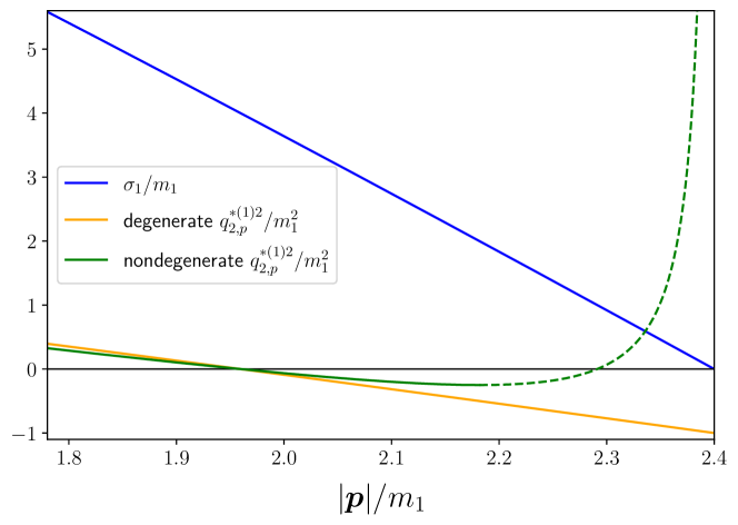
Figure 1: Dependence of $\sigma_{1}/m_{1}^{2}$ (solid blue) and $q_{2,p}^{*(1)2}/m_{1}^{2}$ (solid orange, and green solid/dashed) on $|\boldsymbol{p}|/m_{1}$ for $E=5m_{1}$ and $\boldsymbol{P}=0$. Here $\boldsymbol{p}$ is the momentum of the spectator, which has flavor $1$. The initial proposal for the cutoff function, given in Eq. 22, vanishes at the point where $\sigma_{i}=0$, which corresponds to the maximum value of $|\boldsymbol{p}|/m_{1}$ used. The two curves for $q_{2,p}^{*(1)2}/m_{1}^{2}$ are for $m_{2}=m_{3}=m_{1}$ (orange curve) and for $m_{2}=0.5m_{1},m_{3}=1.5m_{1}$ (green), respectively. The latter curve is shown as dashed after the minimum, which occurs at the position of the left-hand cut, as discussed in the text.

The above-described problem can be avoided by lowering the cutoff in the nondegenerate case, in such a way that $q_{2,p}^{*(i)2}$ does not extend beyond its minimum. This is illustrated in Figure 1 by the transition from a solid to a dashed line for the nondegenerate curve. Using the expression in Eq. 11, it is straightforward to show that the minimum occurs when $q_{2,p}^{*(i)2}=-m_{{\rm min},jk}^{2}$, where $m_{{\rm min},jk}$ is the smaller of $m_{j}$ and $m_{k}$, or equivalently when $\sigma_{i}=|m_{k}^{2}-m_{j}^{2}|$. To implement this choice, we propose defining

$$H^{(i)}(\boldsymbol{p}) =J(z^{\prime}_{i})\,,$$ (27)

$$z^{\prime}_{i} \equiv(1+\epsilon_{H})\frac{\sigma_{i}-|m_{j}^{2}-m_{k}^{2}|}{(m_{j}+m_{k})^{2}-|m_{j}^{2}-m_{k}^{2}|}=(1+\epsilon_{H})\frac{\sigma_{i}-|m_{j}^{2}-m_{k}^{2}|}{2m_{{\rm min},jk}(m_{j}+m_{k})}\,.$$ (28)

which agrees with the standard form in Eq. 22 in the degenerate limit. We have used the new form in practice in the numerical examples shown below. We set $\epsilon_{H}=0$, since, although in theory this can lead to additional power-law volume effects, they are suppressed in practice by the fact that the interpolation function $J(z)$ remains very close to unity for a range of $z$ below unity. For example $1-J(0.92)\approx 4\times 10^{-6}$.

We have described the need for the lowered cutoff in pragmatic terms. There is, however, an additional reason for this choice that is based on the underlying physics. This is the position of the left-hand cut in $\mathcal{K}_{2}$, which is inherited from that in $\mathcal{M}_{2}$. This nonanalyticity arises because of cuts in the $t$ and $u$ channels, which occur for subthreshold kinematics in the $s$ channel. The derivation of the quantization condition accounts for $s$-channel cuts, but not those in $t$ and $u$ channels. Indeed, the resultant nonanalyticities invalidate the derivation of the three-particle quantization condition, where subthreshold two-particle contributions are important. Thus one must either deal with them explicitly in a yet-to-be-developed manner, or place the cutoff so that they are avoided. The $t$-channel cut occurs when $t_{2}=4m_{{\rm min},jk}^{2}$ and $s_{2}=u_{2}=|m_{j}^{2}-m_{k}^{2}|$, where the subscripts on $s_{2}$, $t_{2}$, and $u_{2}$ indicate that they apply to a two-particle subchannel. The $u$-channel cut has the same position except with $t_{2}\leftrightarrow u_{2}$. In both cases, $\sigma_{i}=s_{2}=|m_{j}^{2}-m_{k}^{2}|$, which we recognize as the same position as where $q_{2,p}^{*(i)2}$ reaches its minimum. Thus the cutoff function given in Eq. 27 avoids the left-hand cut, and the quantization condition remains strictly valid.

It might be thought problematic that a lower cutoff is required for the nondegenerate theory—it certainly conflicts with the usual notion of a UV cutoff that one can send arbitrarily large, a point stressed recently in Ref. Muller:2021uur . This is why we have also called $H^{(i)}$ a “transition function,” because, in all derivations in the RFT approach, it has the effect of transitioning the two-particle amplitude that appears in the expressions between the two-particle K matrix $\mathcal{K}_{2}$ at threshold (where $H^{(i)}=1$) and the two-particle amplitude $\mathcal{M}_{2}$ far below threshold (where $H^{(i)}=0$). As the discussion in this section has shown, the presence of the left-hand cut implies that, within the context of a derivation that does not explicitly account for the impact of the associated nonanalyticities, the region of the transition cannot be extended further below threshold. We stress that there is nothing inconsistent in this situation: the fact that the cutoff lies a distance below threshold that is set by $m_{{\rm min},jk}$ implies that the exponentially suppressed corrections that are not controlled behave as $\exp(-m_{{\rm min},jk}L)$. This is the expected size of such corrections, which are dropped throughout the derivation. In practice, when studying the $\pi\pi K$ and $\pi KK$ systems, this implies that the cutoff, in terms of $q_{2,p}^{*(i)2}$, must be placed at the same position as in the study of the $3\pi$ system, since the minimum mass is that of the pion in all cases.

2.3 Implementation of threshold expansion of ${\mathcal{K}_{\mathrm{df},3}}$

In this section we describe how we determine the form of the matrix $\widehat{\mathcal{K}}_{\mathrm{df},3}$ that enters the quantization condition [Eq. 2]. The starting point is the result for the infinite-volume amplitude ${\mathcal{K}_{\mathrm{df},3}}$. We label the initial momenta as $p_{1}$, $p_{1^{\prime}}$, and $p_{2}$, and the final momenta as $p^{\prime}_{1}$, $p^{\prime}_{1^{\prime}}$, and $p^{\prime}_{2}$, with the subscripts indicating the flavor. All these momenta are on shell, and the total four-momentum is $(E,\boldsymbol{P})$. Using the invariance of ${\mathcal{K}_{\mathrm{df},3}}$ under Lorentz transformations, under interchange of the two identical particles separately in the initial and final state, and under time reversal and parity, it was shown in Ref. Blanton:2021mih that, to linear order in the threshold expansion,

$${\mathcal{K}_{\mathrm{df},3}}=\mathcal{K}_{\mathrm{df},3}^{{\rm iso},0}+\mathcal{K}_{\mathrm{df},3}^{{\rm iso},1}\Delta+\mathcal{K}_{\mathrm{df},3}^{B,1}\Delta_{2}^{S}+\mathcal{K}_{\mathrm{df},3}^{E,1}\widetilde{t}_{22}\,.$$ (29)

Here $\mathcal{K}_{\mathrm{df},3}^{{\rm iso},0}$, $\mathcal{K}_{\mathrm{df},3}^{{\rm iso},1}$, $\mathcal{K}_{\mathrm{df},3}^{B,1}$, and $\mathcal{K}_{\mathrm{df},3}^{E,1}$ are real constants, while the dimensionless kinematic variables are given by

$$\begin{split}\Delta&=\frac{s-M}{M^{2}}\,,\quad s=(p_{1}+p_{1^{\prime}}+p_{2})^{2}=P^{2}\,,\\ \Delta_{2}^{S}&=\Delta_{2}+\Delta^{\prime}_{2}\,,\quad\Delta_{2}=\frac{(p_{1}+p_{1^{\prime}})^{2}-4m_{1}^{2}}{M^{2}}\,,\quad\Delta^{\prime}_{2}=\frac{(p^{\prime}_{1}+p^{\prime}_{1^{\prime}})^{2}-4m_{1}^{2}}{M^{2}}\,,\\ \widetilde{t}_{22}&=\frac{t_{22}}{M^{2}}=\frac{(p_{2}-p^{\prime}_{2})^{2}}{M^{2}}\,,\end{split}$$ (30)

where $M=2m_{1}+m_{2}$. In the threshold expansion $\Delta\sim\Delta_{2}^{S}\sim\widetilde{t}_{22}$ are assumed small compared to unity. As we will see explicitly below, working to linear order in the threshold expansion implies that only $s$- and $p$-wave contributions are present, i.e. $\ell\leq 1$ and $\ell^{\prime}\leq 1$.

The matrix appearing in the quantization condition is Blanton:2021mih

$$\widehat{\mathcal{K}}_{\mathrm{df},3}=\begin{pmatrix}[\mathcal{K}_{\mathrm{df},3}]_{p\ell^{\prime}m^{\prime}1;k\ell m1}&[\mathcal{K}_{\mathrm{df},3}]_{p\ell^{\prime}m^{\prime}1;k\ell m2}/\sqrt{2}\\ [\mathcal{K}_{\mathrm{df},3}]_{p\ell^{\prime}m^{\prime}2;k\ell m1}/\sqrt{2}&[\mathcal{K}_{\mathrm{df},3}]_{p\ell^{\prime}m^{\prime}2;k\ell m2}/2\end{pmatrix}\,.$$ (31)

Each of the four entries corresponds to a different decomposition of ${\mathcal{K}_{\mathrm{df},3}}$, differing in the flavors of the spectators. To explain how this decomposition is defined, we consider the example of the top-right or flavor “12” entry. In this case, the outgoing spectator momentum has flavor 1, so that $\boldsymbol{p}=\boldsymbol{p}_{1}$, while the incoming spectator momentum has flavor 2, implying $\boldsymbol{k}=\boldsymbol{p}_{2}$. In the final state, the remaining pair has flavors $1^{\prime}$ and $2$, and the remaining kinematic degree of freedom (for fixed $E$, $\boldsymbol{P}$, and $\boldsymbol{p}_{1}$) is the direction of $\boldsymbol{p}^{\prime}_{1^{\prime}}$ when boosted to the CMF of the pair, which is denoted $\widehat{a}^{\prime*}$. Similarly, in the initial state, the pair has flavors $1$ and $1^{\prime}$, and the remaining degree of freedom is the direction of $\boldsymbol{p}_{1}$ in the incoming pair CMF, and this is denoted $\widehat{a}^{*}$. To proceed, we first express ${\mathcal{K}_{\mathrm{df},3}}$ in terms of these kinematic variables, and then decompose into spherical harmonics as follows

$${\mathcal{K}_{\mathrm{df},3}}(\boldsymbol{p},\widehat{a}^{\prime*};\boldsymbol{k},\widehat{a}^{*})=\sum_{\ell^{\prime}m^{\prime},\ell m}4\pi Y_{\ell^{\prime}m^{\prime}}(\widehat{a}^{\prime*})[{\mathcal{K}_{\mathrm{df},3}}]_{p\ell^{\prime}m^{\prime}1;k\ell m2}Y_{\ell m}(\widehat{a}^{*})\,.$$ (32)

This is a straightforward but tedious exercise, and we sketch its results below. The other decompositions are obtained following the same procedure with different choices of spectator flavors.

One immediate general result is that only even values of angular momenta can be present if the spectator momentum has flavor $2$, because the remaining pair consists of identical particles. Since $\ell_{\rm max}=1$ for our choice of ${\mathcal{K}_{\mathrm{df},3}}$, this implies that, if the flavor index is $2$, only $\ell=m=0$ contributions are present in the decompositions. Only if the flavor index is $1$ can both $\ell=0$ and $1$ terms appear.

The decomposition of the first two terms in Eq. 29 is trivial. These are isotropic, i.e., they only depend on the total CMF energy and not on the directions of the three particles. Thus there is no dependence on $\widehat{a}^{\prime*}$ or $\widehat{a}^{*}$ in any of the decompositions, so only $\ell^{\prime}=\ell=0$ terms appear. Given the normalization choice in Eq. 32, we thus find that the nonzero contributions are

$$[{\mathcal{K}_{\mathrm{df},3}}]_{p001;k001}=[{\mathcal{K}_{\mathrm{df},3}}]_{p001;k002}=[{\mathcal{K}_{\mathrm{df},3}}]_{p002;k001}=[{\mathcal{K}_{\mathrm{df},3}}]_{p002;k002}\supset\mathcal{K}_{\mathrm{df},3}^{{\rm iso},0}+\mathcal{K}_{\mathrm{df},3}^{{\rm iso},1}\Delta\,.$$ (33)

We stress that these results hold for all choices of the spectator momenta $\boldsymbol{p}$ and $\boldsymbol{k}$.

Since the decompositions of the other two terms in ${\mathcal{K}_{\mathrm{df},3}}$ require more explanation, we will address them in separate subsections below. Before doing so, however, we comment on two general issues. The first concerns the removal of factors of $q^{*}$ from the quantization condition. As noted in Sec. 2, we can do so by making the replacement $\widehat{\mathcal{K}}_{\mathrm{df},3}\to\widehat{Q}^{-1}\widehat{\mathcal{K}}_{\mathrm{df},3}\widehat{Q}^{-1}$. The implementation of this transformation on the decompositions described below is very straightforward: one simply deletes all appearances of $a^{*}\equiv|\boldsymbol{a}^{*}|$ and $a^{\prime*}\equiv|\boldsymbol{a}^{\prime*}|$.

Second, we note that a useful check of the decompositions, and their implementation in the code, is obtained from the fact that the underlying quantity ${\mathcal{K}_{\mathrm{df},3}}$ is Lorentz invariant. It follows that the different blocks of $\widehat{\mathcal{K}}_{\mathrm{df},3}$ in Eq. 31 are themselves invariant if we transform $P=(E,\boldsymbol{P})$, $p$, and $k$ with a common, arbitrary, boost, aside from the need to apply a Wigner D-matrix rotation to the parts of the decomposition with $\ell^{\prime}=1$ and/or $\ell=1$. The need for these extra rotations is discussed in Sec. VII of Ref. Blanton:2020gmf . We have checked our decompositions in this manner.

2.3.1 Decomposition of the $\mathcal{K}_{\mathrm{df},3}^{B,1}$ contribution

We begin with the flavor $22$ decomposition [the bottom-right block in Eq. 31] as we know that this involves only $\ell^{\prime}=\ell=0$. Since $\boldsymbol{p}=\boldsymbol{p}^{\prime}_{2}$ and $\boldsymbol{k}=\boldsymbol{p}_{2}$ in this case, we have that

$$M^{2}\Delta_{2}=(P-k)^{2}-4m_{1}^{2}\ \ {\rm and}\ \ M^{2}\Delta^{\prime}_{2}=(P-p)^{2}-4m_{1}^{2}\,.$$ (34)

Explicitly evaluating the inner products leads to the contribution

$$M^{2}[\mathcal{K}_{\mathrm{df},3}]_{p002;k002}\supset 2\mathcal{K}_{\mathrm{df},3}^{B,1}[s-E(\omega_{p}^{(2)}+\omega_{k}^{(2)})+\boldsymbol{P}\cdot(\boldsymbol{p}+\boldsymbol{k})+m_{2}^{2}-4m_{1}^{2}]\,.$$ (35)

We stress that this differs from the isotropic contribution to the same element, given in Eq. 33, because it depends not only on $s$ but also on the spectator momenta.

Next we turn to the flavor $11$ decomposition [the top-left block in Eq. 31], which is the most complicated. Since now $\boldsymbol{p}=\boldsymbol{p}^{\prime}_{1}$ and $\boldsymbol{k}=\boldsymbol{p}_{1}$, we have

$$\begin{split}M^{2}\Delta_{2}&=2p_{1}\cdot p_{1^{\prime}}-2m_{1}^{2}=k\cdot p_{+}+k\cdot p_{-}-2m_{1}^{2}\,,\\ M^{2}\Delta^{\prime}_{2}&=2p^{\prime}_{1}\cdot p^{\prime}_{1^{\prime}}-2m_{1}^{2}=p\cdot p^{\prime}_{+}+p\cdot p^{\prime}_{-}-2m_{1}^{2}\,,\\ p_{\pm}&=p_{1^{\prime}}\pm p_{2}\,,\quad p^{\prime}_{\pm}=p^{\prime}_{1^{\prime}}\pm p^{\prime}_{2}\,.\end{split}$$ (36)

The $p_{+}$ and $p^{\prime}_{+}$ terms are simple to evaluate given that $p_{+}=P-k$ and $p^{\prime}_{+}=P-p$, and do not depend on the pair CMF directions. The $p_{-}$ and $p^{\prime}_{-}$ terms do, however, depend on these directions, because, in their respective pair CMFs, we have

$$p_{-} =(p_{-,0}^{*},2\boldsymbol{a}^{*})\,,\quad p^{*}_{-,0}=\omega_{a^{*}}^{(1)}-\omega_{a^{*}}^{(2)}\,,$$ (37)

$$p^{\prime}_{-} =(p^{\prime*}_{-,0},2\boldsymbol{a}^{\prime*})\,,\quad p^{\prime*}_{-,0}=\omega_{a^{\prime*}}^{(1)}-\omega_{a^{\prime*}}^{(2)}\,.$$ (38)

To evaluate the $k\cdot p_{-}$ term, for example, we must boost the lab-frame four-vector ${k=(\omega_{k}^{(1)},\boldsymbol{k})}$ into the CMF of the initial state $1^{\prime}2$ pair. This requires a boost with velocity ${\boldsymbol{\beta}_{k}=-(\boldsymbol{P}-\boldsymbol{k})/(E-\omega_{k}^{(1)})}$, and, using the notation introduced in Sec. 2.1, leads to

$$k\xrightarrow{\textrm{boost by }\boldsymbol{\beta}_{k}}\left(\omega_{k^{*k}}^{(1)},\boldsymbol{k}^{*(11^{\prime}k)}\right)\,,\qquad\omega_{k^{*k}}^{(1)}\equiv\sqrt{m_{1}^{2}+|\boldsymbol{k}^{*(11^{\prime}k)}|^{2}}\,.$$ (39)

Similarly, for the $p\cdot p^{\prime}_{-}$ term, we need the boost of $p$ by $\boldsymbol{\beta}_{p}$,

$$p\xrightarrow{\textrm{boost by }\boldsymbol{\beta}_{p}}\left(\omega_{p^{*p}}^{(1)},\boldsymbol{p}^{*(11^{\prime}p)}\right)\,,\qquad\omega_{p^{*p}}^{(1)}\equiv\sqrt{m_{1}^{2}+|\boldsymbol{p}^{*(11^{\prime}p)}|^{2}}\,.$$ (40)

Using these results we now have

$$\begin{split}M^{2}\Delta_{2}&=E\omega_{k}^{(1)}-\boldsymbol{k}\cdot\boldsymbol{P}-3m_{1}^{2}+\omega_{k^{*k}}^{(1)}p^{*}_{-,0}-2\boldsymbol{k}^{*(11^{\prime}k)}\cdot\boldsymbol{a}^{*}\,,\\ M^{2}\Delta^{\prime}_{2}&=E\omega_{p}^{(1)}-\boldsymbol{p}\cdot\boldsymbol{P}-3m_{1}^{2}+\omega_{p^{*p}}^{(1)}p^{\prime*}_{-,0}-2\boldsymbol{p}^{*(11^{\prime}p)}\cdot\boldsymbol{a}^{\prime*}\,,\end{split}$$ (41)

so that the dependence on the CMF directions is explicit.

To decompose the terms linear in $\boldsymbol{a}^{*}$ and $\boldsymbol{a}^{\prime*}$, we use

$$\boldsymbol{p}\cdot\boldsymbol{a}=\frac{4\pi}{3}pa\sum_{m}Y_{1m}(\widehat{p})Y_{1m}(\widehat{a})\,.$$ (42)

This allows us to pull out the spherical harmonics in the decomposition of the flavor 11 term that is analogous to Eq. 32, and thus to read off

$$\begin{split}M^{2}[\mathcal{K}_{\mathrm{df},3}]_{p001;k001}&\supset\mathcal{K}_{\mathrm{df},3}^{B,1}[E(\omega_{p}^{(1)}\!+\!\omega_{k}^{(1)})\!-\!(\boldsymbol{p}\!+\!\boldsymbol{k})\cdot\boldsymbol{P}\!-\!6m_{1}^{2}\!+\!\omega_{k^{*k}}^{(1)}p^{*}_{-,0}\!+\!\omega_{p^{*p}}^{(1)}p^{\prime*}_{-,0}]\,,\\ M^{2}[\mathcal{K}_{\mathrm{df},3}]_{p1m^{\prime}1;k001}&\supset-2\mathcal{K}_{\mathrm{df},3}^{B,1}\frac{a^{\prime*}}{3}\mathcal{Y}_{1m^{\prime}}(\boldsymbol{p}^{*(11^{\prime}p)})\,,\\ M^{2}[\mathcal{K}_{\mathrm{df},3}]_{p001;k1m1}&\supset-2\mathcal{K}_{\mathrm{df},3}^{B,1}\frac{a^{*}}{3}\mathcal{Y}_{1m}(\boldsymbol{k}^{*(11^{\prime}k)})\,.\end{split}$$ (43)

Here we are using the harmonic polynomials defined in Eq. 10. We observe that there are no contributions with $\ell^{\prime}=\ell=1$.

The flavor off-diagonal entries of $\widehat{\mathcal{K}}_{\mathrm{df},3}$ can be obtained from the results above, and we find

$$\begin{split}M^{2}[\mathcal{K}_{\mathrm{df},3}]_{p001;k002}&\supset\mathcal{K}_{\mathrm{df},3}^{B,1}[E\omega_{p}^{(1)}\!-\!\boldsymbol{p}\cdot\boldsymbol{P}\!+\!s\!-\!2E\omega_{k}^{(2)}\!+\!2\boldsymbol{P}\cdot\boldsymbol{k}\!+\!\omega_{p^{*p}}^{(1)}p^{\prime*}_{-,0}\!+\!m_{2}^{2}\!-\!7m_{1}^{2}]\,,\\ M^{2}[\mathcal{K}_{\mathrm{df},3}]_{p1m^{\prime}1;k002}&\supset-2\mathcal{K}_{\mathrm{df},3}^{B,1}\frac{a^{\prime*}}{3}\mathcal{Y}_{1m^{\prime}}(\boldsymbol{p}^{*(11^{\prime}p)})\,,\\ M^{2}[\mathcal{K}_{\mathrm{df},3}]_{p002;k001}&\supset\mathcal{K}_{\mathrm{df},3}^{B,1}[E\omega_{k}^{(1)}\!-\!\boldsymbol{k}\cdot\boldsymbol{P}\!+\!s\!-\!2E\omega_{p}^{(2)}\!+\!2\boldsymbol{P}\cdot\boldsymbol{p}\!+\!\omega_{k^{*k}}^{(1)}p^{*}_{-,0}\!+\!m_{2}^{2}\!-\!7m_{1}^{2}]\,,\\ M^{2}[\mathcal{K}_{\mathrm{df},3}]_{p002;k1m1}&\supset-2\mathcal{K}_{\mathrm{df},3}^{B,1}\frac{a^{*}}{3}\mathcal{Y}_{1m}(\boldsymbol{k}^{*(11^{\prime}k)})\,.\end{split}$$ (44)

2.3.2 Decomposition of the $\mathcal{K}_{\mathrm{df},3}^{E,1}$ contribution

The 22 block is simple to obtain using $t_{22}=2m_{2}^{2}-2p^{\prime}_{2}\cdot p_{2}$, which leads to

$$M^{2}[\mathcal{K}_{\mathrm{df},3}]_{p002;k002}\supset 2\mathcal{K}_{\mathrm{df},3}^{E,1}[m_{2}^{2}-\omega_{p}^{(2)}\omega_{k}^{(2)}+\boldsymbol{p}\cdot\boldsymbol{k}]\,.$$ (45)

For the flavor 11 block, we need to rewrite $t_{22}$ in terms of $p_{\pm}$ and $p^{\prime}_{\pm}$,

$$t_{33} \to 2m_{2}^{2}-\frac{1}{2}\left(p^{\prime}_{+}\cdot p_{+}+p^{\prime}_{-}\cdot p_{-}-p^{\prime}_{+}\cdot p_{-}-p^{\prime}_{-}\cdot p_{+}\right)\,.$$ (46)

To evaluate this we need

$$\begin{split}p^{\prime}_{+}\cdot p_{+}&=(P\!-\!p)\cdot(P\!-\!k)=s-E(\omega_{p}^{(1)}+\omega_{k}^{(1)})+\boldsymbol{P}\cdot(\boldsymbol{p}+\boldsymbol{k})+\omega_{p}^{(1)}\omega_{k}^{(1)}-\boldsymbol{p}\cdot\boldsymbol{k}\,,\\ p^{\prime}_{+}\cdot p_{-}&=(P\!-\!p)_{0}^{*(11^{\prime}k)}p^{*}_{-,0}-2(\boldsymbol{P}\!-\!\boldsymbol{p})^{*(11^{\prime}k)}\cdot\boldsymbol{a}^{*}\,,\\ p^{\prime}_{-}\cdot p_{+}&=p^{\prime*}_{-,0}(P\!-\!k)_{0}^{*(11^{\prime}p)}-2\boldsymbol{a}^{\prime*}\cdot(\boldsymbol{P}\!-\!\boldsymbol{k})^{*(11^{\prime}p)}\,.\end{split}$$ (47)

Here $(P\!-\!p)_{0}^{*(11^{\prime}k)}$ is the energy component of the four-vector $p^{\prime}_{+}=P-p$ boosted by $\boldsymbol{\beta}_{k}$, while $(P\!-\!k)_{0}^{*(11^{\prime}p)}$ is the energy component of $p_{+}=P-k$ boosted by $\boldsymbol{\beta}_{p}$.

To obtain $p^{\prime}_{-}\cdot p_{-}$ we need to boost the four-vectors $p_{-}$ and $p^{\prime*}_{-}$, given in Eqs. 37 and 38 in their respective CMFs, into the lab frame. After doing so, we find

$$p^{\prime}_{-}\cdot p_{-}=\gamma_{k}\gamma_{p}(1-\boldsymbol{\beta}_{k}\cdot\boldsymbol{\beta}_{p})p^{\prime*}_{-,0}p^{*}_{-,0}+2\boldsymbol{a}^{*}\cdot\boldsymbol{V}+2\boldsymbol{a}^{\prime*}\cdot\boldsymbol{V}^{\prime}+4a^{\prime*}_{i}T_{ij}a^{*}_{j}\,,$$ (48)

where

$$\boldsymbol{V} =\left[\boldsymbol{\beta}_{p}\gamma_{p}+\widehat{\beta}_{k}\widehat{\beta}_{k}\cdot\boldsymbol{\beta}_{p}(\gamma_{k}\!-\!1)\gamma_{p}-\boldsymbol{\beta}_{k}\gamma_{k}\gamma_{p}\right]p^{\prime*}_{-,0}\,,$$

$$\boldsymbol{V}^{\prime} =\left[\boldsymbol{\beta}_{k}\gamma_{k}+\widehat{\beta}_{p}\widehat{\beta}_{p}\cdot\boldsymbol{\beta}_{k}(\gamma_{p}\!-\!1)\gamma_{k}-\boldsymbol{\beta}_{p}\gamma_{p}\gamma_{k}\right]p^{*}_{-,0}\,,$$ (49)

$$T_{ij} =\widehat{\beta}_{p,i}\widehat{\beta}_{k,j}\left[\gamma_{p}\gamma_{k}\beta_{p}\beta_{k}-\widehat{\beta}_{p}\cdot\widehat{\beta}_{k}(\gamma_{p}\!-\!1)(\gamma_{k}\!-\!1)\right]-\widehat{\beta}_{p,i}\widehat{\beta}_{p,j}(\gamma_{p}\!-\!1)-\widehat{\beta}_{k,i}\widehat{\beta}_{k,j}(\gamma_{k}\!-\!1)-\delta_{ij}\,.$$

Thus we observe the first appearance of a term linear in both $\boldsymbol{a}^{\prime}$ and $\boldsymbol{a}^{\prime*}$, which gives a contribution with $\ell^{\prime}=\ell=1$.

To proceed, we note that

$$a^{\prime*}_{i}T_{ij}a^{*}_{j}=\frac{1}{3}\mathcal{Y}_{1m^{\prime}}(\boldsymbol{a}^{\prime*})T_{m^{\prime}m}\mathcal{Y}_{1m}(\boldsymbol{a}^{*})\,.$$ (50)

where $T_{m^{\prime}m}$ is defined by converting $T_{ij}$ into the spherical basis, i.e. with $m=1$, $0$, and $-1$ corresponding to $j=x$, $z$, and $y$, respectively. Using this, and the results above, we find

$$\begin{split}\hfil\displaystyle\begin{split}M^{2}[\mathcal{K}_{\mathrm{df},3}]_{p001;k001}&\supset\mathcal{K}_{\mathrm{df},3}^{E,1}\Big{\{}2m_{2}^{2}-\frac{1}{2}\big{[}s-E(\omega_{p}^{(1)}\!+\!\omega_{k}^{(1)})+\boldsymbol{P}\cdot(\boldsymbol{p}\!+\!\boldsymbol{k})+\omega_{p}^{(1)}\omega_{k}^{(1)}-\boldsymbol{p}\cdot\boldsymbol{k}\\ &\quad-(P\!-\!p)_{0}^{*(11^{\prime}k)}p^{*}_{-,0}-(P\!-\!k)_{0}^{*(11^{\prime}p)}p^{\prime*}_{-,0}+\gamma_{k}\gamma_{p}(1\!-\!\boldsymbol{\beta}_{k}\cdot\boldsymbol{\beta}_{p})p^{\prime*}_{-,0}p^{*}_{-,0}\big{]}\Big{\}}\,,\end{split}\\ M^{2}[\mathcal{K}_{\mathrm{df},3}]_{p1m^{\prime}1;k001}&\supset-\mathcal{K}_{\mathrm{df},3}^{E,1}\frac{a^{\prime*}}{3}\mathcal{Y}_{1m^{\prime}}(\boldsymbol{P}^{*(11^{\prime}p)}-\boldsymbol{k}^{*(11^{\prime}p)}+\boldsymbol{V}^{\prime})\,,\\ M^{2}[\mathcal{K}_{\mathrm{df},3}]_{p001;k1m1}&\supset-\mathcal{K}_{\mathrm{df},3}^{E,1}\frac{a^{*}}{3}\mathcal{Y}_{1m}(\boldsymbol{P}^{*(11^{\prime}k)}-\boldsymbol{p}^{*(11^{\prime}k)}+\boldsymbol{V})\,,\\ M^{2}[\mathcal{K}_{\mathrm{df},3}]_{p1m^{\prime}1;k1m1}&\supset-\mathcal{K}_{\mathrm{df},3}^{E,1}\frac{2a^{\prime*}a^{*}}{3}T_{m^{\prime}m}\,.\end{split}$$ (51)

Finally we come to the off-diagonal terms. For the upper-right block, we need

$$\begin{split}t_{22}&=2m_{2}^{2}-(p^{\prime}_{+}-p^{\prime}_{-})\cdot p_{2}\\ &=2m_{2}^{2}-(P-p)\cdot k+p^{\prime*}_{-,0}\omega_{k^{*p}}^{(2)}-2\boldsymbol{a}^{\prime*}\cdot\boldsymbol{k}^{*(11^{\prime}p)}\,,\end{split}$$ (52)

where $\omega_{k^{*p}}^{(2)}$ is the energy of an on-shell particle of flavor 2 with momentum $\boldsymbol{k}^{*(11^{\prime}p)}$. For the lower-left block, we need

$$t_{22} =2m_{2}^{2}-p\cdot(P-k)+p^{*}_{-,0}\omega_{p^{*k}}^{(2)}-2\boldsymbol{p}^{*(11^{\prime}k)}\cdot\boldsymbol{a}^{*}\,.$$ (53)

We can now read off

$$\begin{split}M^{2}[\mathcal{K}_{\mathrm{df},3}]_{p001;k002}&\supset\mathcal{K}_{\mathrm{df},3}^{E,1}[2m_{2}^{2}-(E-\omega_{p}^{(1)})\omega_{k}^{(2)}+(\boldsymbol{P}-\boldsymbol{p})\cdot\boldsymbol{k}+p^{\prime*}_{-,0}\omega_{k^{*p}}^{(2)}]\,,\\ M^{2}[\mathcal{K}_{\mathrm{df},3}]_{p1m^{\prime}1;k002}&\supset-\mathcal{K}_{\mathrm{df},3}^{E,1}\frac{2a^{\prime*}}{3}\mathcal{Y}_{1m^{\prime}}(\boldsymbol{k}^{*(11^{\prime}p)})\,.\\ M^{2}[\mathcal{K}_{\mathrm{df},3}]_{p002;k001}&\supset\mathcal{K}_{\mathrm{df},3}^{E,1}[2m_{2}^{2}-\omega_{p}^{(2)}(E-\omega_{k}^{(1)})+\boldsymbol{p}\cdot(\boldsymbol{P}-\boldsymbol{k})+p^{*}_{-,0}\omega_{p^{*k}}^{(2)}]\,,\\ M^{2}[\mathcal{K}_{\mathrm{df},3}]_{p002;k1m1}&\supset-\mathcal{K}_{\mathrm{df},3}^{E,1}\frac{2a^{*}}{3}\mathcal{Y}_{1m}(\boldsymbol{p}^{*(11^{\prime}k)})\,.\end{split}$$ (54)

2.4 Irrep projections

In order to compare solutions of the quantization condition to a physical finite-volume spectrum obtained from lattice QCD, one must first classify the solutions into the irreps of the appropriate symmetry group of the system, namely the little group of transformations of the cube that leave the total momentum $\boldsymbol{P}$ invariant:

$$\text{LG}(\boldsymbol{P})\equiv\{R\in O_{h}|R\boldsymbol{P}=\boldsymbol{P}\}\,,$$ (55)

where $O_{h}$ is the full cubic group with 48 elements. As in previous works (e.g. Refs. Blanton:2019igq ; Blanton:2019vdk ), we accomplish this by projecting the matrices appearing in the quantization condition onto individual irrep subspaces. Unlike in those papers, however, here we have the additional complication of nondegenerate particle flavors, which adds a layer of structure to the projection matrices.

In order to interpret some of the results that we present here and in Sec. A.3, it is useful to list the little groups for each of the classes of total momenta. We collect these, along with the irreps, in Table 1.

$\boldsymbol{d}_{\rm ref}$	$\text{LG}(\boldsymbol{P})$	irreps
$(0,0,0)$	$O_{h}$	$A_{1g}[1],A_{2g}[1],E_{g}[2],T_{1g}[3],T_{2g}[3],A_{1u}[1],A_{2u}[1],E_{u}[2],T_{1u}[3],T_{2u}[3]$
$(0,0,n)$	$C_{4v}$	$A_{1}[1],\,A_{2}[1],\,B_{1}[1],\,B_{2}[1],\,E[2]$
$(n,n,0)$	$C_{2v}$	$A_{1}[1],\,A_{2}[1],\,B_{1}[1],\,B_{2}[1]$
$(n,n,n)$	$C_{3v}$	$A_{1}[1],\,A_{2}[1],\,E[2]$
$(n_{1},n_{2},0)$	$C_{2}$	$A_{1}[1],\,A_{2}[1]$
$(n_{1},n_{1},n_{2})$	$C_{2}$	$A_{1}[1],\,A_{2}[1]$
$(n_{1},n_{2},n_{3})$	$C_{1}$	$A_{1}[1]$

Table 1: Little group $\text{LG}(\boldsymbol{P})$ for each type of frame, along with its irreps, each with its dimension listed in square brackets. Frames are denoted by $\boldsymbol{d}_{\rm def}=\boldsymbol{P}L/(2\pi)$, taking a canonical choice for each type of frame. The integers $n$, $n_{1}$, $n_{2}$, and $n_{3}$ are nonzero, with $n_{1}$, $n_{2}$, and $n_{3}$ being distinct.

For a 2+1 system of pseudoscalars (e.g. $\pi\pi K$, $KK\pi$) at fixed $L$ and ${P=(E,\boldsymbol{P})}$, each matrix $\widehat{M}\in\{\widehat{F},\widehat{G},\widehat{\overline{\mathcal{K}}}_{2,L},\widehat{F}_{3},\widehat{\mathcal{K}}_{\mathrm{df},3}\}$ used in the quantization condition is invariant under a set of orthogonal transformation matrices $\{\widehat{U}(R)\}_{R\in\text{LG}(\boldsymbol{P})}$:

$$\widehat{U}(R)^{T}\widehat{M}\widehat{U}(R) =\widehat{M}\qquad\forall R\in\text{LG}(\boldsymbol{P})\,,$$ (56)

$$[\widehat{U}(R)]_{p\ell^{\prime}m^{\prime}i;k\ell mj} \equiv\delta_{ij}\delta_{\boldsymbol{p},R\boldsymbol{k}}\delta_{\ell^{\prime}\ell}\Pi(R)\mathcal{D}^{(\ell)}_{m^{\prime}m}(R)\,,$$ (57)

where $\mathcal{D}^{(\ell)}(R)$ is a real-basis Wigner D-matrix, and $\Pi(R)$ is the parity of transformation $R$, i.e. $+1$ if $R$ is a pure rotation and $-1$ otherwise. The latter factor appears because we consider pseudoscalar mesons; to describe scalars one replaces $\Pi(R)\to 1$. The feature of these matrices that is new to this work is the added flavor structure. Note that $\widehat{U}(R)$ is diagonal in its flavor and partial-wave indices, as well as block diagonal in its spectator-momentum indices, with the momenta in a given block all belonging to the same finite-volume “orbit” $o_{\boldsymbol{k}}\equiv\{R\boldsymbol{k}|R\in\text{LG}(\boldsymbol{P})\}$.

The transformation matrices furnish a (reducible) representation of $\text{LG}(\boldsymbol{P})$:

$$\widehat{U}(R_{1}R_{2})=\widehat{U}(R_{1})\widehat{U}(R_{2})\quad\forall R_{1},R_{2}\in\text{LG}(\boldsymbol{P})\,,\qquad\widehat{U}(\boldsymbol{1}_{3})=\boldsymbol{1}\,,$$ (58)

which can be decomposed into irreps $I$ via projection matrices

$$\widehat{P}_{I}\equiv\frac{d_{I}}{[\text{LG}(\boldsymbol{P})]}\sum_{R\in\text{LG}(\boldsymbol{P})}\chi_{I}(R)\widehat{U}(R)\,,$$ (59)

where $[\text{LG}(\boldsymbol{P})]$ is the cardinality of the little group, $d_{I}$ is the dimension of irrep $I$, and $\chi_{I}(R)$ is its character. Lastly, we collect the eigenvectors of $\widehat{P}_{I}$ with nonzero (unit) eigenvalue into a smaller, non-square matrix $\widehat{P}_{I,\text{sub}}$, which projects $\widehat{M}$ onto the lower-dimensional irrep subspace,

$$\widehat{M}_{I,\text{sub}} =(\widehat{P}_{I,\text{sub}})^{T}\widehat{M}\widehat{P}_{I,\text{sub}}\,.$$ (60)

The eigenvalues of $\widehat{M}_{I,\text{sub}}$ are precisely the subset of the eigenvalues of $\widehat{M}$ that lie in irrep $I$. Thus the quantization condition Eq. 2 can be rewritten as

$$\det\left[\widehat{F}_{3}^{-1}+\widehat{\mathcal{K}}_{\mathrm{df},3}\right] =\prod_{I}\det\left[\left(\widehat{F}_{3}^{-1}+\widehat{\mathcal{K}}_{\mathrm{df},3}\right)_{I,\text{sub}}\right]=0\,,$$ (61)

allowing for irrep-by-irrep comparisons between solutions to the quantization condition and the physical finite-volume spectrum.

Although the projection matrices $\{\widehat{P}_{I}\}$ have the same diagonal and block-diagonal index structure as the $\{\widehat{U}(R)\}_{R\in\text{LG}(\boldsymbol{P})}$, the quantization condition matrix $\widehat{F}_{3}^{-1}+\widehat{\mathcal{K}}_{\mathrm{df},3}$ generally does not, mixing together different flavors, partial waves, and spectator orbits in its eigenvalues and eigenvectors. We discuss the details of eigenvalue decomposition into different irreps in Sec. A.3.

We close this section by listing in Table 2 the irreps (and corresponding number of eigenvalues) affected by the nonisotropic terms in ${\mathcal{K}_{\mathrm{df},3}}$ and by $\widehat{\overline{\mathcal{K}}}_{2,L}$. We also show the two-particle irreps in the two-particle quantization condition that are affected by $\mathcal{K}_{2}^{(i)}$, when one considers nonidentical particles and includes both $s$ and $p$ waves. By comparing to Table 1, one can see which irreps are not affected by either of these interactions. We do not list the results for the cases that are trivial. These are the two-particle quantization condition for identical particles with only $s$-wave interactions, and the three-particle quantization condition with isotropic terms in ${\mathcal{K}_{\mathrm{df},3}}$, for both of which there is only a single nonzero eigenvalue that lies in the trivial irrep. As shown in the table, it turns out that the nonisotropic $\mathcal{K}_{\mathrm{df},3}^{B,1}$ term does not affect any of the nontrivial irreps. These only enter in the decompositions of the $\mathcal{K}_{\mathrm{df},3}^{E,1}$ term (some irreps) and of $\widehat{\overline{\mathcal{K}}}_{2,L}$ (all irreps). The fact that $\widehat{\overline{\mathcal{K}}}_{2,L}$ couples to all available irreps follows from the results that it is a diagonal matrix with, in general, nonzero entries in all positions, and that it is proportional to the identity matrix in each of the orbits listed in Sec. A.3. This implies that, for large enough $L$, it contains all irreps, irrespective of the maximum value of $\ell$.

$\boldsymbol{d}_{\rm ref}$	$\mathcal{K}_{2}^{(1)}$ (QC2)	$\mathcal{K}_{\mathrm{df},3}^{B,1}$ (QC3)	$\mathcal{K}_{\mathrm{df},3}^{E,1}$ (QC3)	$\widehat{\overline{\mathcal{K}}}_{2,L}$ (QC3)
$(0,0,0)$	$A_{1g}(1),\,T_{1u}(3)$	$A_{1u}(2)$	$A_{1u}(2),\,T_{1g}(3)$	all
$(0,0,n)$	$A_{1}(2),\,E(2)$	$A_{2}(2)$	$A_{2}(3),\,E(2)$	all
$(n,n,0)$	$A_{1}(2),\,B_{1}(1),\,B_{1}(1)$	$A_{2}(2)$	$A_{2}(3),\,B_{1}(1),\,B_{2}(1)$	all
$(n,n,n)$	$A_{1}(2),\,E(2)$	$A_{2}(2)$	$A_{2}(3),\,E(2)$	all
$(n_{1},n_{2},0)$	$A_{1}(3),\,A_{2}(1)$	$A_{2}(2)$	$A_{2}(4),\,A_{1}(1)$	all
$(n_{1},n_{1},n_{2})$	$A_{1}(3),\,A_{2}(1)$	$A_{2}(2)$	$A_{2}(4),\,A_{1}(1)$	all
$(n_{1},n_{2},n_{3})$	$A_{1}(4)$	$A_{1}(2)$	$A_{1}(5)$	all

Table 2: Irrep decompositions of the eigenvalues of two- and three-particles K matrices for different frames, and for both two- and three-particle quantization conditions (denoted QC2 and QC3, respectively). Frames are denoted as in Table 1. Results assume both $s$- and $p$-wave dimers in the flavor-1 spectator channel and only $s$ waves in the flavor-2 channel, and are for the $L\to\infty$ limit. For finite $L$ and energies in the range of validity of the quantization condition, some of the eigenvalues may be absent; see Sec. A.3 for further discussion. The notation $I(n)$ denotes that there are $n$ nonzero eigenvalues in irrep $I$, a number that includes the multiplicity of the irrep. In assigning irreps, all particles are assumed to be pseudoscalars, so that, for example, the trivial irreps of two- and three-particle systems are the parity complements of each other. The description “all” in the final column indicates that there are nonzero eigenvalues in every irrep that is present for a given choice of $E$, particle masses, and $L$. Which irreps are present can be determined from the tables in Sec. A.3. We observe that, aside from the final column, the total number of nonzero eigenvalues of each K matrix is independent of frame, as expected of a Lorentz-invariant object.

3 ${\mathcal{K}_{\mathrm{df},3}}$ from chiral perturbation theory

The goal of this section is to work out the leading-order (LO) prediction in ChPT for ${\mathcal{K}_{\mathrm{df},3}}$ for the $2+1$ systems of interest for this work: $\pi^{+}\pi^{+}K^{+}$ and $\pi^{+}K^{+}K^{+}$. This is a generalization of the calculation for $3\pi^{+}$ carried out in Ref. Blanton:2019vdk , and involves only minor additional technical complications arising from the presence of nonidentical particles.

In fact, ${\mathcal{K}_{\mathrm{df},3}}$ cannot be directly calculated in ChPT. Instead, one must calculate the physical three-particle scattering amplitude $\mathcal{M}_{3}$, and then use the relation between $\mathcal{M}_{3}$ and ${\mathcal{K}_{\mathrm{df},3}}$. In general, the latter involves solving integral equations, but at LO in ChPT the relation only involves subtracting certain divergent terms from $\mathcal{M}_{3}$. The details of this relation for identical particles are given in Ref. Hansen:2015zga , and the generalization to the 2+1 system is outlined in Ref. Blanton:2021mih . In Appendix C we present a detailed description, the result of which is that

$$\mathcal{K}_{\mathrm{df},3}^{\rm LO}=\mathcal{M}_{\text{df,3}}^{\rm LO}\equiv\mathcal{M}_{3}^{\rm LO}-\mathcal{D}^{\rm LO}\,,$$ (62)

where the subtraction term $\mathcal{D}^{\rm LO}$ is given in Eq. 148.

We use the standard $N_{f}=3$ ChPT Lagrangian:

$$\mathcal{L}=\frac{F^{2}}{4}{\rm tr}\left[\partial_{\mu}U\partial_{\mu}U^{\dagger}\right]+\frac{BF^{2}}{2}{\rm tr}\left[\hat{m}_{q}\left(U+U^{\dagger}\right)\right]\,,$$ (63)

with $U=\exp\left(i{\phi}/{F}\right)$, $F\approx 93\;$MeV the pseudoscalar decay constant, and

$$\phi=\begin{pmatrix}\pi^{0}+\frac{1}{\sqrt{3}}\eta&\sqrt{2}\pi^{+}&\sqrt{2}K^{+}\\ \sqrt{2}\pi^{-}&-\pi^{0}+\frac{1}{\sqrt{3}}\eta&\sqrt{2}K^{0}\\ \sqrt{2}K^{-}&\sqrt{2}\overline{K}^{0}&-\frac{2}{\sqrt{3}}\eta\end{pmatrix}\,.$$ (64)

We work in the isosymmetric limit, in which $\hat{m}_{q}=\text{diag }(m_{l},m_{l},m_{s})$. The LO pion and kaon masses are given by

$$M_{\pi}^{2}=2m_{l}B\,,\qquad M_{K}^{2}=(m_{l}+m_{s})B\,.$$ (65)

3.1 Calculation of $\mathcal{M}_{3}$

We use the same notation as in Sec. 2.3, labeling the incoming and outgoing momenta $p_{i}$ and $k_{i}$, respectively, with $i=1,1^{\prime},2$. The two identical particles correspond to $i=1$ and $1^{\prime}$, with mass $m_{1}$, while the third corresponds to $i=2$, with mass $m_{2}$. Thus $(m_{1},m_{2})=(M_{\pi},M_{K})$ and $(M_{K},M_{\pi})$ correspond respectively to the $\pi^{+}\pi^{+}K^{+}$ and $\pi^{+}K^{+}K^{+}$ systems.

There are three different types of diagrams that contribute, as shown in Figure 2. The first two are one-particle exchange (OPE) diagrams, in which the exchanged particle can either be of flavor 1 [diagram (a)] or flavor 2 [diagram (b)]. Both OPE diagrams appear four times, with different momentum labels or ordering of vertices. In addition, there is a contact term resulting from the six-meson vertex [diagram (c)].

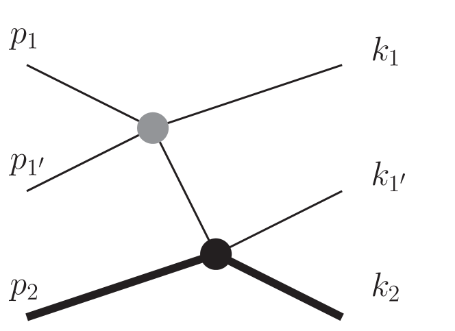
(a)

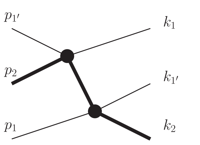
(b)

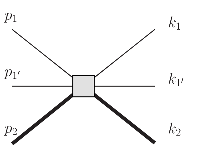
(c)

Figure 2: Diagrams contributing to $\mathcal{M}_{3}^{\rm LO}$. Thin (thick) lines indicate particles of flavor 1 (2). Four-particle vertices are denoted by circles: black if the particles are of different flavors, grey if all particles are of flavor 1. The gray square indicates the six-particle vertex.

As can be seen explicitly by expanding the chiral Lagrangian in Eq. 63, the terms contributing to $\pi^{+}\pi^{+}$ and $K^{+}K^{+}$ scattering are formally identical up to $\pi\leftrightarrow K$ relabelling. The same holds for $\pi^{+}\pi^{+}K^{+}$ and $\pi^{+}K^{+}K^{+}$ scattering. Thus we can treat both systems simultaneously without specifying the choice of $(m_{1},m_{2})$.

We find that the contribution from diagram (a) is given by

$$\mathcal{M}_{3}^{(a)}=-\mathcal{M}_{2}^{(2)\text{,off1}}(p_{1},p_{1^{\prime}})\frac{1}{b^{2}_{(a)}-m_{1}^{2}+i\epsilon}\mathcal{M}_{2}^{(1)\text{,off1}}(k_{1^{\prime}},k_{2}),\quad b_{(a)}=p_{1}+p_{1^{\prime}}-k_{1},$$ (66)

where the off-shell two-particle amplitudes are given by

$$\begin{split}\mathcal{M}_{2}^{(2)\text{,off1}}(p_{1},p_{1^{\prime}})=&-\frac{2p_{1}\cdot p_{1^{\prime}}}{F^{2}}+\frac{1}{3F^{2}}(b_{(a)}^{2}-m_{1}^{2})\,,\\ \mathcal{M}_{2}^{(1)\text{,off1}}(k_{1^{\prime}},k_{2})=&-\frac{k_{1^{\prime}}\cdot k_{2}}{F^{2}}+\frac{1}{6F^{2}}(b_{(a)}^{2}-m_{1}^{2})\,.\end{split}$$ (67)

The notation “off1” indicates that it is a particle of flavor 1 that is off shell. For diagram (b) the result is similar,

$$\mathcal{M}_{3}^{(b)}=-\mathcal{M}_{2}^{(1)\text{,off2}}(p_{1^{\prime}},p_{2})\frac{1}{b^{2}_{(b)}-m_{2}^{2}+i\epsilon}\mathcal{M}_{2}^{(1)\text{,off2}}(k_{1^{\prime}},k_{2})\,,\quad b_{(b)}=p_{1^{\prime}}+p_{2}-k_{1}\,,$$ (68)

where

$$\mathcal{M}_{2}^{(1)\text{,off2}}(k_{1^{\prime}},k_{2})= -\frac{k_{1^{\prime}}\cdot k_{2}}{F^{2}}+\frac{1}{6F^{2}}(b_{(b)}^{2}-m_{2}^{2})\,,$$ (69)

with the particle of flavor 2 being off shell.

As noted above, the full contribution of the OPE diagrams to $\mathcal{M}_{3}^{\rm LO}$ requires the addition of other terms. For diagram (a) one adds the result of interchanging $k_{1}$ and $k_{1^{\prime}}$, and for both resulting diagrams one adds the result of a PT transformation, which is obtained by making the interchanges $k_{i}\leftrightarrow p_{i}$. For diagram (b), one interchanges flavors $1$ and $1^{\prime}$ for both initial and final states. We hold off on adding these other contributions until we have made the subtractions.

Finally, for the diagram with the six-point vertex we find

$$F^{4}\mathcal{M}_{3}^{(c)}=\frac{1}{3}M^{2}\Delta-\frac{1}{36}M^{2}\Delta_{2}^{S}+\frac{1}{12}M^{2}\widetilde{t}_{22}+\frac{2}{3}\left(2m_{1}m_{2}+m_{1}^{2}\right)\,,$$ (70)

where we are using the kinematic quantities defined in Eq. 30. We stress that no subtraction is needed for this contribution.

3.2 Subtraction terms and $\mathcal{M}_{\mathrm{df},3}$

We next evaluate $\mathcal{D}^{\rm LO}$, which is given in Eq. 148. The terms on the first two lines of this result subtract the contributions from OPE diagrams of type Figure 2(a), while those on the third line contain the subtractions for diagrams of type Figure 2(b). We stress that the subtraction can be done diagram by diagram. The results for the subtraction terms are very similar to those for the original diagrams, except that the off-shell two-particle amplitudes are replaced by their on-shell correspondents. Thus, for example, the subtraction term for Figure 2(a) is

$$\mathcal{D}^{(a)}=-\mathcal{M}_{2}^{(2)\text{,on}}(p_{1},p_{1^{\prime}})\frac{1}{b_{(a)}^{2}-m_{1}^{2}+i\epsilon}\mathcal{M}_{2}^{(1)\text{,on}}(k_{1^{\prime}},k_{2})\,,$$ (71)

where

$$\begin{split}\mathcal{M}_{2}^{(2)\text{,on}}(p_{1},p_{1^{\prime}})=-\frac{2p_{1}\cdot p_{1^{\prime}}}{F^{2}},\quad\mathcal{M}_{2}^{(1)\text{,on}}(k_{1^{\prime}},k_{2})=-\frac{k_{1^{\prime}}\cdot k_{2}}{F^{2}}\,.\end{split}$$ (72)

Similarly, for diagram (b) one simply drops the $b_{(b)}^{2}-m_{2}^{2}$ contributions in the expression for $\mathcal{M}_{2}^{(1),\rm off2}$, Eq. 69.

Using these results, we obtain the divergence-free matrix elements

$$F^{4}\mathcal{M}_{\text{df,3}}^{(a)} =\frac{1}{3}(p_{1}\cdot p_{1^{\prime}}+k_{1^{\prime}}\cdot k_{2})-\frac{1}{18}(b_{(a)}^{2}-m_{1}^{2})\,,$$ (73)

$$F^{4}\mathcal{M}_{\text{df,3}}^{(b)} =\frac{1}{6}(p_{1^{\prime}}\cdot p_{2}+k_{1^{\prime}}\cdot k_{2})-\frac{1}{36}(b_{(b)}^{2}-m_{2}^{2})\,.$$ (74)

If we now add to these the above-described three additional contributions for each type of diagram, we find

$$F^{4}\mathcal{M}_{\text{df,3}}^{(a),\text{all}} =\frac{M^{2}}{18}\left(6\Delta+3\Delta_{2}^{S}-2\widetilde{t}_{22}\right)+\frac{4}{3}(m_{1}m_{2}+m_{1}^{2})\,,$$ (75)

$$F^{4}\mathcal{M}_{\text{df,3}}^{(b),\text{all}} =\frac{M^{2}}{36}\left(12\Delta-5\Delta_{2}^{S}+\widetilde{t}_{22}\right)+\frac{4}{3}m_{1}m_{2}\,.$$ (76)

3.3 Final result

At this point we note that the contribution from each of the three diagrams, i.e. those from Eqs. 70, 75 and 76, has the form expected, based on symmetries, given in Eq. 29. There are isotropic terms with either no dependence or linear dependence on $s$ (or, equivalently, on $\Delta$), together with nonisotropic $\Delta_{2}^{S}$ and $\widetilde{t}_{22}$ terms. We note that working to LO in ChPT leads to contributions with up to two powers of momenta, which are thus at most linear in the Mandelstam variables. Thus it corresponds to working to linear order in the threshold expansion described in Sec. 2.3.

However, when we combine the three contributions to get the final result, we find that the nonisotropic terms cancel

$$F^{4}\mathcal{K}_{\mathrm{df},3}^{\rm LO} =F^{4}\left(\mathcal{M}_{\text{df,3}}^{(a),\text{all}}+\mathcal{M}_{\text{df,3}}^{(b),\text{all}}+\mathcal{M}_{3}^{(c)}\right)$$ (77)

$$=M^{2}\Delta+4m_{1}m_{2}+2m_{1}^{2}\,.$$ (78)

We do not have an explanation for this cancellation. It implies that the contributions to the coefficients of the nonisotropic terms, i.e. $\mathcal{K}_{\mathrm{df},3}^{B,1}$ and $\mathcal{K}_{\mathrm{df},3}^{E,1}$ in Eq. 29, can appear first at NLO in ChPT. Thus while $\mathcal{K}_{\mathrm{df},3}^{{\rm iso},0}\sim\mathcal{K}_{\mathrm{df},3}^{{\rm iso},1}\sim m^{2}/F^{4}$, we expect that $\mathcal{K}_{\mathrm{df},3}^{B,1}\sim\mathcal{K}_{\mathrm{df},3}^{E,1}\sim m^{4}/F^{6}$, where $m$ is a generic meson mass.

4 Numerical applications

In this section we provide two numerical applications of the quantization conditions that we have implemented. First, we compare the energy of the ground state of a completely nondegenerate system with the $1/L$ expansion derived in Appendix B. Our aims here are to provide a check of our numerical implementation (which must agree increasingly well with the truncated $1/L$ expansion as $L$ increases) and to see how rapidly the $1/L$ expansion converges. We choose the nondegenerate system both to advertise that the code for this is available, and also because the threshold expansion for this system has not previously been derived.

In our second example, we use the $2+1$ quantization condition to predict the energy shifts for several levels in the $\pi\pi K$ and $KK\pi$ systems, choosing parameters that are likely to be used in near-term lattice simulations. Our main aim here is to illustrate the precision needed to determine the different components of $\mathcal{K}_{2}$ and ${\mathcal{K}_{\mathrm{df},3}}$.

4.1 Testing the threshold expansion

The expansion of the energy of the ground state when the total momentum vanishes is usually referred to as the “threshold expansion.” In Appendix B we obtain the following result for the threshold expansion for three nondegenerate scalars,

$$\begin{split}L^{3}\Delta E&=\sum_{i=1}^{3}\frac{2\pi a_{0}^{(i)}}{\mu_{i}}\left[1-\frac{a_{0}^{(i)}}{\pi L}\mathcal{I}+\left(\frac{a_{0}^{(i)}}{\pi L}\right)^{2}(\mathcal{I}^{2}-\mathcal{J})+\frac{a^{(j)}_{0}a^{(k)}_{0}}{(\pi L)^{2}}2\mathcal{J}\right]+O(L^{-6})\,,\end{split}$$ (79)

where $i$, $j$, and $k$ are ordered cyclically, $\mu_{i}$ is the reduced mass of the $jk$ system, and $a^{(k)}_{0}$ is the scattering length of particles $i$ and $j$.

To test our implementation of the nondegenerate quantization condition, we choose the following mass ratios

$$\frac{m_{2}}{m_{1}}=1.5,\quad\frac{m_{3}}{m_{1}}=0.5\,.$$ (80)

We express all quantities in units of the mass of the first particle, $m_{1}$, including the size of the box $m_{1}L$. Since the effective range does not enter the threshold expansion until $O(1/L^{6})$, we keep only the leading term in the effective-range expansion for the phase shift

$$q\cot\delta^{(ij)}_{0}=-\frac{1}{a_{0}^{(k)}}.$$ (81)

Similarly, since neither $p$-wave two-particle interactions nor ${\mathcal{K}_{\mathrm{df},3}}$ enters into the threshold expansion until higher order, we consider the quantization condition with only $s$ waves and with ${\mathcal{K}_{\mathrm{df},3}}=0$. We choose the following values for the scattering lengths,

$$m_{1}a_{0}^{(1)}=0.7,\quad m_{1}a_{0}^{(2)}=0.5,\quad m_{1}a_{0}^{(3)}=0.3.$$ (82)

Our choices in Eqs. 80 and 82 imply significant nondegeneracy in masses, and symmetry breaking in interactions. In this way we are performing a fairly robust test of our implementation.

The numerical results are shown in Figure 3. The left plot shows the dependence of the energy shift on the size of the box. We observe that, while the leading-order result captures the overall behavior of the exact results, albeit with a noticeable offset, adding in the $O(L^{-4})$ and $O(L^{-5})$ terms leads to a much closer agreement. To study this more quantitatively, we show in the right plot the difference between the numerical and analytical results,

$$\delta E\equiv|\left(\Delta E\right)^{\rm QC3}-\left(\Delta E\right)^{\rm th}|.$$ (83)

For small $m_{1}L$ it appears that the threshold expansion truncated at the $L^{-4}$ term does better than that including the $L^{-5}$ term, indicating a breakdown in convergence. However, at the largest volumes shown the expected ordering of curves sets in. This gives us confidence in our implementation, and also indicates that relatively large volumes are needed for the threshold expansion to give a good approximation to the energy shift.

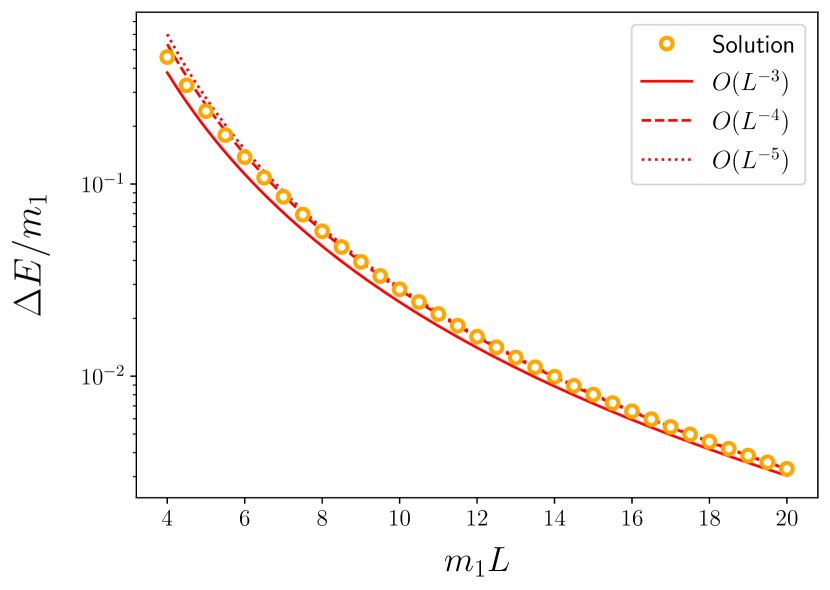
(a)

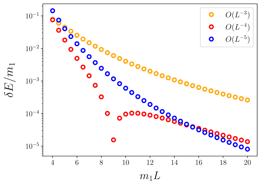
(b)

Figure 3: Numerical comparison between the results from the quantization condition and the threshold expansion. (a) Energy shift as a function of the box size. Orange dots show the numerical solutions to the quantization condition, while the various red lines are the theoretical predictions of Eq. 79, truncated to different orders in the $1/L$ expansion. (b) Box-size dependence of the quantity in Eq. 83, which is the absolute value of the difference between the threshold expansion at various orders and the numerical solution as a function of $m_{1}L$.

4.2 Model results for the $\pi^{+}\pi^{+}K^{+}$ and $\pi^{+}K^{+}K^{+}$ energy levels

A major motivation for developing the formalism for $2+1$ systems was that extensive lattice results for such systems will be available soon. Specifically, recent lattice calculations of multiple energy levels for $3\pi^{+}$ and $3K^{+}$ systems Horz:2019rrn ; Culver:2019vvu ; Fischer:2020jzp ; Hansen:2020otl ; Alexandru:2020xqf ; Brett:2021wyd ; Blanton:2021llb can be relatively straightforwardly generalized to $\pi^{+}\pi^{+}K^{+}$ and $\pi^{+}K^{+}K^{+}$. The only previous study of the latter systems of which we are aware considered the threshold states alone Detmold:2011kw .

An important consideration when fitting the quantization condition to results for the spectrum is the precision needed from the lattice calculation in order to determine the various parameters that enter $\mathcal{K}_{2}$ and ${\mathcal{K}_{\mathrm{df},3}}$. Here we give an indication of the required precision for $\pi^{+}\pi^{+}K^{+}$ and $\pi^{+}K^{+}K^{+}$ systems. Specifically, we determine the energy shift for several levels in the rest frame and a moving frame. These levels are in several irreps of the cubic group (which is the symmetry group of the cubic box that we consider). We choose the $\pi^{+}$ and $K^{+}$ masses from the N203 ensemble Bruno:2016plf created by the Coordinated Lattice Simulations (CLS) effort, which is one of the ensembles used in the recent detailed analysis of $3\pi^{+}$ and $3K^{+}$ systems in Ref. Blanton:2021llb . The parameters that we need are

$$M_{K}/M_{\pi}=1.278,\quad M_{\pi}/F_{\pi}=3.433,\quad M_{K}/F_{K}=4.153,\quad M_{\pi}L=5.4053,$$ (84)

where $M_{\pi}$ and $F_{\pi}$ are the pion mass and decay constant, and $M_{K}$ and $F_{K}$ the analogous quantities for the kaon.

To make predictions for the energy shifts, we set $\mathcal{K}_{2}$ and ${\mathcal{K}_{\mathrm{df},3}}$ to their LO expressions in SU(3) ChPT, which we expect will be a reasonable approximation for levels that are not at too high energies. This implies that all interactions are purely $s$-wave. The $\pi^{+}\pi^{+}$ and $K^{+}K^{+}$ phase shifts are given by

$$\frac{q}{M_{\pi}}\cot\delta^{\pi\pi}_{0} =\frac{M_{\pi}\sqrt{s}}{s-2M_{\pi}^{2}}\left(-\frac{16\pi F_{\pi}^{2}}{M_{\pi}^{2}}\right),$$ (85)

$$\frac{q}{M_{K}}\cot\delta^{KK}_{0} =\frac{M_{K}\sqrt{s}}{s-2M_{K}^{2}}\left(-\frac{16\pi F_{K}^{2}}{M_{K}^{2}}\right)\,,$$ (86)

where $s$ is the two-particle squared total four-momentum. At LO in ChPT $F=F_{\pi}=F_{K}$, and we have chosen the decay constant corresponding to the particles that are scattering. For $\pi^{+}K^{+}$ scattering the LO expression can be written

$$\frac{q}{M_{\pi}}\cot\delta^{\pi K}_{0}=\frac{M_{\pi}\sqrt{s}}{s-M_{\pi}^{2}-M_{K}^{2}}\left(-\frac{16\pi F_{\pi}^{2}}{M_{\pi}^{2}}\right)\,,$$ (87)

which we use in the $\pi^{+}\pi^{+}K^{+}$ case, or

$$\frac{q}{M_{K}}\cot\delta^{\pi K}_{0}=\frac{M_{K}\sqrt{s}}{s-M_{\pi}^{2}-M_{K}^{2}}\left(-\frac{16\pi F_{K}^{2}}{M_{K}^{2}}\right)\,,$$ (88)

which we use for $\pi^{+}K^{+}K^{+}$. Note that the choice of $M_{\pi}$ or $M_{K}$ to make quantities dimensionless is arbitrary, since the overall factors of mass cancel. We also note that the cutoff function described in Sec. 2.2 implies that we will evaluate $\delta^{\pi K}_{0}$ down to $s_{\text{min}}=M_{K}^{2}-M_{\pi}^{2}$, where $q^{2}=-M_{\pi}^{2}$. By contrast, $\delta^{\pi\pi}_{0}$ and $\delta^{KK}_{0}$ will be evaluated down to $s_{\text{min}}=0$, where $q^{2}=-M_{\pi}^{2}$ and $q^{2}=-M_{K}^{2}$, respectively.

For ${\mathcal{K}_{\mathrm{df},3}}$ we use the results of Sec. 3. Again we have to choose which decay constants to use in the LO expressions, and our approach is to divide each particle mass by the corresponding decay constant. In this way we obtain from Eq. 78 the following LO results

$$M_{\pi}^{2}\mathcal{K}_{\text{df,3}}^{\pi\pi K} =2\frac{M_{\pi}^{4}}{F_{\pi}^{4}}+4\frac{M_{\pi}^{3}}{F_{\pi}^{3}}\frac{M_{K}}{F_{K}}+\frac{M_{\pi}^{2}}{F_{\pi}^{2}}\left(2\frac{M_{\pi}}{F_{\pi}}+\frac{M_{K}}{F_{K}}\right)^{2}\Delta\,,$$ (89)

$$M_{K}^{2}\mathcal{K}_{\text{df,3}}^{KK\pi} =2\frac{M_{K}^{4}}{F_{K}^{4}}+4\frac{M_{K}^{3}}{F_{K}^{3}}\frac{M_{\pi}}{F_{\pi}}+\frac{M_{K}^{2}}{F_{K}^{2}}\left(2\frac{M_{K}}{F_{K}}+\frac{M_{\pi}}{F_{\pi}}\right)^{2}\Delta\,.$$ (90)

Using these inputs we then numerically solve the quantization condition and determine the shifts of the CMF energy $E^{*}=\sqrt{E^{2}-\boldsymbol{P}^{2}}$ for each level from the corresponding free energy. These shifts are plotted for the several levels in Figure 4 as the points denoted “LO ChPT.” These are all the levels that appear in the lowest three orbits in the rest frame and the first moving frame. For reference, the CMF energies of these levels are collected in Table 3.

$\boldsymbol{d}_{\rm ref}$	$[d_{1}^{2},d_{1^{\prime}}^{2},d_{2}^{2}]$	irreps	$E^{*\rm free}_{\pi\pi K}/M_{\pi}$	$E^{*\rm free}_{\pi KK}/M_{K}$
(0, 0, 0)	[0, 0, 0]	$A_{1u}$	3.278	2.782
	[0, 1, 1]	$A_{1u}\oplus E_{u}\oplus T_{1g}$	4.260	3.486
	[1, 1, 0]	$E_{u}\oplus T_{1g}$	4.345	3.552
(0, 0, 1)	[0, 0, 1]	$A_{2}$	3.542	2.999
	[0, 1, 0]	$A_{2}$	3.630	3.068
	[0, 1, 2]	$A_{2}\oplus B_{2}\oplus E$	4.467	3.652

Table 3: Noninteracting CMF energies, $E^{*\rm free}=\sqrt{E_{\rm free}^{2}-\boldsymbol{P}^{2}}$, and little group irreps, for the $\pi^{+}\pi^{+}K^{+}$ and $\pi^{+}K^{+}K^{+}$ levels appearing in Figure 4. Frames are denoted by $\boldsymbol{d}_{\rm ref}={\boldsymbol{P}}L/(2\pi)$. Orbits are specified by the squared momenta of the three particles, e.g. $d_{1}^{2}=\boldsymbol{p}_{1}^{2}(L/(2\pi))^{2}$. The flavor labels are $\{1,1^{\prime},2\}=\{\pi^{+},\pi^{+},K^{+}\}$ for $\pi^{+}\pi^{+}K^{+}$, and $\{1,1^{\prime},2\}=\{K^{+},K^{+},\pi^{+}\}$ for $\pi^{+}K^{+}K^{+}$.

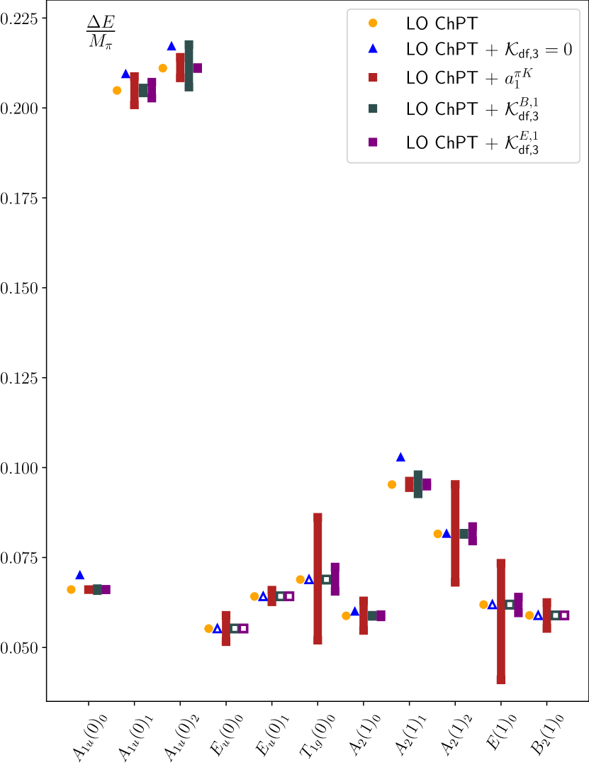
(a)

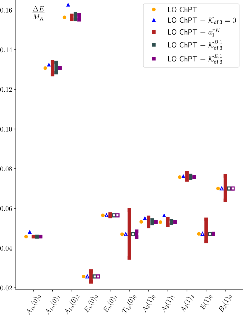
(b)

Figure 4: Shifts in the CMF energy of various levels with different choices of parameters in $\mathcal{K}_{2}$ and ${\mathcal{K}_{\mathrm{df},3}}$ for (a) the $\pi^{+}\pi^{+}K^{+}$ and (b) the $\pi^{+}K^{+}K^{+}$ systems. The levels are denoted along the bottom of the figures using the notation ${\rm irrep}(\boldsymbol{d}_{\rm ref}^{2})_{\rm level}$, where $\boldsymbol{d}_{\rm ref}=\boldsymbol{P}L/(2\pi)$ describes the frame, while the subscript $0,1,\dots$ denotes the level, with $0$ being the ground state in the given irrep and frame. For each level, there are five points, as discussed in the text.

Since leading-order two-particle interactions give the dominant contribution to the energy shifts, an important question is how large are the effects of higher-order two- and three-particle interactions on the energy shifts. To answer this question, we include, for each level, four more points in Figure 4. The first shows the effect of setting ${\mathcal{K}_{\mathrm{df},3}}=0$ while keeping the $s$-wave phase shifts unchanged. We observe that some levels do not depend at all on the isotropic ${\mathcal{K}_{\mathrm{df},3}}$ predicted by LO ChPT, whereas for the others there is a shift. To determine the isotropic component of ${\mathcal{K}_{\mathrm{df},3}}$ one needs to determine the energy shifts with errors no larger than $\sim 5\%$. This precision has been achieved for some levels in the $3\pi^{+}$ and $3K^{+}$ spectra of Ref. Blanton:2021llb .

The remaining three points for each level in Figure 4 display the impact of terms of higher order in ChPT. The first considers the $p$-wave $\pi^{+}K^{+}$ interaction, which appears at NLO in ChPT. To estimate the size of the $p$-wave scattering length (defined in Eq. 17) we use the NLO SU(3) ChPT results from Ref. Bernard:1990kw from which it follows that

$$Ma_{1}^{\pi K}\sim\frac{1}{16\pi F^{2}}\frac{M^{2}}{(4\pi F)^{2}}\,,$$ (91)

where the unknown overall constant of $\mathcal{O}(1)$ arises from a combination of loops and low-energy coefficients, and $M$ represents a combination of pion and kaon masses that varies from term to term. To implement this in practice we choose

$$M_{\pi}^{3}a_{1}^{\pi K}=c\frac{M_{\pi}+M_{K}}{2M_{\pi}M_{K}}\frac{M_{\pi}^{2}}{(4\pi F_{\pi})^{2}}\left(\frac{M_{\pi}^{2}}{(4\pi F_{\pi})^{2}}+\frac{M_{K}^{2}}{(4\pi F_{K})^{2}}\right)\,,$$ (92)

for the $\pi^{+}\pi^{+}K^{+}$ system, and

$$M_{K}^{3}a_{1}^{\pi K}=c\frac{M_{\pi}+M_{K}}{2M_{\pi}M_{K}}\frac{M_{K}^{2}}{(4\pi F_{K})^{2}}\left(\frac{M_{\pi}^{2}}{(4\pi F_{\pi})^{2}}+\frac{M_{K}^{2}}{(4\pi F_{K})^{2}}\right)\,,$$ (93)

for the $\pi^{+}K^{+}K^{+}$ system. We vary $c$ in the range $-3\leq c\leq 3$, which corresponds, after keeping track of factors of $\pi$, to the overall constant in Eq. 91 being $\sim 1$. This leads to the bands shown as the third (maroon) entry for each level in Figure 4. We note that all levels are sensitive to $a_{1}^{\pi K}$, and that for most, though not all, the sensitivity is greater than that to the LO part of ${\mathcal{K}_{\mathrm{df},3}}$.

Finally we consider the NLO contributions to ${\mathcal{K}_{\mathrm{df},3}}$. Both $\mathcal{K}_{\mathrm{df},3}^{B,1}$ and $\mathcal{K}_{\mathrm{df},3}^{E,1}$ appear at this order; we choose

$$M_{\pi}^{2}{\mathcal{K}^{B,1}_{\mathrm{df},3}}=c_{B}\frac{M_{\pi}^{4}}{F_{\pi}^{4}}\frac{M_{K}^{2}}{F_{K}^{2}}\,,\qquad M_{\pi}^{2}{\mathcal{K}^{E,1}_{\mathrm{df},3}}=c_{E}\frac{M_{\pi}^{4}}{F_{\pi}^{4}}\frac{M_{K}^{2}}{F_{K}^{2}}$$ (94)

for the $\pi^{+}\pi^{+}K^{+}$ system, and

$$M_{K}^{2}{\mathcal{K}^{B,1}_{\mathrm{df},3}}=c_{B}\frac{M_{\pi}^{2}}{F_{\pi}^{2}}\frac{M_{K}^{4}}{F_{K}^{4}}\,,\qquad M_{K}^{2}{\mathcal{K}^{E,1}_{\mathrm{df},3}}=c_{E}\frac{M_{\pi}^{2}}{F_{\pi}^{2}}\frac{M_{K}^{4}}{F_{K}^{4}}$$ (95)

for the $\pi^{+}K^{+}K^{+}$ system. We then vary the constants in the range $-1\leq c_{B},c_{E}\leq 1$. Given that the standard estimate of NLO effects involves a loop factor of $1/(4\pi)^{2}$, which we are not including here, these are very aggressive ranges. We justify them by the observation that, if we were to use the analogous chiral estimates for the $d$-wave contributions to ${\mathcal{K}_{\mathrm{df},3}}$ in the $3\pi^{+}$ and $3K^{+}$ systems, then to match the values found in Ref. Blanton:2021llb , a similarly aggressive estimate would be needed. We also note that the scattering amplitude $\mathcal{M}_{3}$ does not diverge when ${\mathcal{K}_{\mathrm{df},3}}\to\pm\infty$.

The final two points for each level in Figure 4 show the effect of making separate variations as just described in ${\mathcal{K}^{B,1}_{\mathrm{df},3}}$ and ${\mathcal{K}^{E,1}_{\mathrm{df},3}}$. We observe that ${\mathcal{K}^{B,1}_{\mathrm{df},3}}$ contributes only to levels in the trivial irreps, but can contribute as much as the isotropic parts of ${\mathcal{K}_{\mathrm{df},3}}$ and $a_{1}^{\pi K}$ to certain levels. ${\mathcal{K}^{E,1}_{\mathrm{df},3}}$ does contribute to some of the levels in nontrivial irreps, which might make it somewhat simpler to determine than ${\mathcal{K}^{B,1}_{\mathrm{df},3}}$.

5 Conclusions

The goal of this paper is to prepare for the analysis of lattice QCD data for systems involving nondegenerate particles. For this, we have implemented the finite-volume formalism derived in Refs. Blanton:2020gmf ; Blanton:2021mih , i.e., for both fully nondegenerate and $2+1$ systems. We have made our code public in the following repository coderepo . The description of the code, together with some examples, can be found in Appendix D.

While many details are similar to the case of identical particles, several additional technical features arise with nondegenerate particles. These have been discussed in Sec. 2, and include the definition of the sum-minus-integral difference for nonidentical particles, as well as the need for a modified cutoff function. The latter is necessary to avoid the $t$-channel cut, which is displaced with respect to the case of identical particles. Furthermore, odd angular momenta appear when the particles are nondegenerate, and the extension of the group theory to handle $p$-wave interactions is explained in Sec. 2.4.

When implementing the quantization conditions, it is useful to have analytic checks in certain limits. One such check is provided by the expansion of the energy of the three-particle ground state in powers of $1/L$. This has been worked out previously for the identical-particle and $2+1$ systems. Here, in Appendix B, we extend the derivation to the fully nondegenerate case, including terms up to $O(L^{-5})$. We show an example of this check on the implementation for a completely nondegenerate system in Sec. 4.1.

As noted in the Introduction, the immediate application for this formalism is to systems with a mix of light pseudoscalar mesons, in particular $\pi^{+}\pi^{+}K^{+}$ and $\pi^{+}K^{+}K^{+}$. Thus we have focused much of the discussion on such $2+1$ systems. To study them in practice, a parametrization of ${\mathcal{K}_{\mathrm{df},3}}$ is needed. This can be achieved using a systematic expansion about threshold that accounts for all symmetries Blanton:2019igq , and if we work to linear order in this expansion, then only four terms contribute Blanton:2021mih . Two of these involve only two-particle $s$ waves, while the other two also include $p$ waves. Due to the possibility of having different flavors of spectator particles, the decomposition of ${\mathcal{K}_{\mathrm{df},3}}$ into the finite-volume kinematic variables becomes more complicated than that for identical particles, and we have worked this out explicitly in Sec. 2.3. The code for $2+1$ systems that we provide includes this implementation.

The parameters in this threshold expansion of ${\mathcal{K}_{\mathrm{df},3}}$ can, in principle, be predicted in ChPT, with the LO calculation being relatively straightforward. The results can serve as a guide for what to expect when fitting to results from lattice simulations. Thus we have extended the work of Ref. Blanton:2019vdk , in which the LO prediction was worked out for $3\pi^{+}$ scattering, to the $\pi^{+}\pi^{+}K^{+}$ and $\pi^{+}K^{+}K^{+}$ systems. The results, provided in Sec. 3, turn out to be completely isotropic, i.e., both two- and three-particle interactions involve only $s$ waves. Thus two of the four parameters in the threshold expansion are predicted to vanish at LO in ChPT, although all four terms are present at intermediate stages.

The finite-volume spectrum of three particles depends primarily on two-particle interactions, with a subleading contribution from ${\mathcal{K}_{\mathrm{df},3}}$. It is important to understand how large the various contributions are to the spectral levels, in order to determine how precisely one must determine their energies in a simulation. To investigate this, in Sec. 4.2, we explore the impact of the different choices for the two- and three-particle K matrices on selected levels in the $\pi^{+}\pi^{+}K^{+}$ and $\pi^{+}K^{+}K^{+}$ spectra. We use the values of the masses, decay constants, and box size that match those of the N203 CLS ensemble Bruno:2016plf . We use both the LO ChPT predictions, and estimates of NLO contributions based on chiral power counting. The results emphasize the importance of using several frames and levels in all available irreps, in order to determine the two-particle $p$-wave interaction and the nonisotropic terms in ${\mathcal{K}_{\mathrm{df},3}}$.

Finally, we recall the recent analysis in Ref. Blanton:2021llb of $3\pi^{+}$ and $3K^{+}$ systems using hundreds of energy levels in total. It appears that extending this work to mixed systems of $K^{+}$ and $\pi^{+}$ mesons is technically feasible. Fitting the results to the $2+1$ quantization condition that we have implemented here should allow a determination of both the $I=3/2$ $\pi K$ scattering amplitudes in $s$ and $p$ waves as well as some of the terms in ${\mathcal{K}_{\mathrm{df},3}}$. Some new technical challenges will need to be faced, e.g., how to simultaneously fit the spectra of multiple three- and two-particle systems, in this case $3\pi^{+}$, $\pi^{+}\pi^{+}K^{+}$, $\pi^{+}K^{+}K^{+}$, and $3K^{+}$, as well as $\pi^{+}\pi^{+}$, $\pi^{+}K^{+}$, and $K^{+}K^{+}$. An important challenge will be the reliable inclusion of correlations between such a large number of levels.

Appendix A Further details of implementation

In this appendix we provide further technical details of the implementation of the quantization condition for $2+1$ systems, which has been described in Sec. 2.

A.1 Real spherical harmonics

As noted in the main text, in practice we use the real version of spherical harmonics, following Ref. Blanton:2019igq . In this way we do not need to keep track of which harmonics to complex conjugate, and all matrices appearing in the quantization condition are real and symmetric. The real spherical harmonics satisfy the same orthonormality conditions as the more standard complex version. In this work we only need those for $\ell=1$, as well as the standard form for $\ell=0$. The former are

$$pY_{11}(\hat{p})=\sqrt{\frac{3}{4\pi}}p_{x}\,,\quad pY_{10}(\hat{p})=\sqrt{\frac{3}{4\pi}}p_{z}\,,\quad pY_{1-1}(\hat{p})=\sqrt{\frac{3}{4\pi}}p_{y}\,.$$ (96)

A.2 Evaluating $\widetilde{F}^{(i)}$

To evaluate $\widetilde{F}^{(i)}$, Eq. 8, we use the UV regularization introduced in Ref. Kim:2005gf . Dropping exponentially suppressed terms, Eq. 8 can be brought into the form

$$\left[\widetilde{F}^{(i)}\right]_{p^{\prime}\ell^{\prime}m^{\prime};p\ell m} =\frac{\delta_{\boldsymbol{p}^{\prime}\boldsymbol{p}}H^{(i)}(\boldsymbol{p})}{16\pi^{2}L^{4}\omega_{p}^{(i)}(E-\omega_{p}^{(i)})}\left[\sum_{\boldsymbol{n}_{a}}-{\rm PV}\!\!\int d^{3}n_{a}\right]\frac{e^{\alpha(x^{2}-r^{2})}}{x^{2}-r^{2}}\frac{\mathcal{Y}_{\ell^{\prime}m^{\prime}}(\boldsymbol{r})\mathcal{Y}_{\ell m}(\boldsymbol{r})}{x^{\ell^{\prime}+\ell}}\,,$$ (97)

where $\boldsymbol{a}=\boldsymbol{n}_{a}(2\pi/L)$, $x=q_{2,p}^{*(i)}L/(2\pi)$, and $\boldsymbol{r}$ is a vector given in terms of ${\boldsymbol{n}_{pP}=(\boldsymbol{p}-\boldsymbol{P})L/(2\pi)}$ by

$$\boldsymbol{r}=\boldsymbol{n}_{a}+\boldsymbol{n}_{pP}\left[\frac{\boldsymbol{n}_{a}\cdot\boldsymbol{n}_{pP}}{\boldsymbol{n}_{pP}^{2}}\left(\frac{1}{\gamma}-1\right)+\frac{\xi}{\gamma}\right]\,,$$ (98)

where

$$\xi=\frac{1}{2}\left(1+\frac{m_{1}^{2}-m_{2}^{2}}{\sigma_{i}}\right)\,,$$ (99)

and

$$\gamma=\frac{E-\omega_{p}^{(i)}}{\sqrt{\sigma_{i}}}\,.$$ (100)

Ultraviolet regularization is provided by $\alpha>0$ Kim:2005gf , with the dependence on $\alpha$ being exponentially suppressed in $L$. The result (97) agrees with the two-particle nondegenerate result given in Refs. Briceno:2012yi ; Davoudi:2011md ; Fu:2011xz ; Leskovec:2012gb .

To evaluate $\widetilde{F}^{(i)}$, we follow the same method as described in Appendix B of Ref. Blanton:2019igq , except here we have $\ell=0,1$, whereas that work considered $\ell=0,2$. In addition, here we extend the implementation to nonzero $\boldsymbol{P}$. The sum and integral are evaluated for a value of $\alpha$ that is sufficiently small that, based on numerical experiments, the residual dependence on $\alpha$ lies below the desired precision for solving the quantization condition. We typically find that $\alpha=0.5$ is adequate.

The sum in Eq. 97 is evaluated as written, except that in practice, we must introduce a cutoff, $|\boldsymbol{n}|<n_{\rm max}$. We use the same cutoff as described in Appendix B.2 of Ref. Blanton:2019igq , taking the $\ell^{\prime}=\ell=0$ value for all choices of angular momenta. Note that for the determination of the cutoff, the value of $|\boldsymbol{n}_{pP}|$ is not relevant as it lies well below $n_{\rm max}$.

The integral in Eq. 97 can be evaluated analytically, as discussed in Appendix B.1 of Ref. Blanton:2019igq . Focusing on the core integral, we have

$$I^{F}_{\ell^{\prime}m^{\prime};\ell m} ={\rm PV}\!\int d^{3}n_{a}\frac{e^{\alpha(x^{2}-r^{2})}}{x^{2}-r^{2}}4\pi\mathcal{Y}_{\ell^{\prime}m^{\prime}}(\boldsymbol{r})\mathcal{Y}_{\ell m}(\boldsymbol{r})$$ (101)

$$=\gamma\;{\rm PV}\!\int d^{3}r\frac{e^{\alpha(x^{2}-r^{2})}}{x^{2}-r^{2}}4\pi\mathcal{Y}_{\ell^{\prime}m^{\prime}}(\boldsymbol{r})\mathcal{Y}_{\ell m}(\boldsymbol{r})$$ (102)

$$=\delta_{\ell^{\prime}\ell}\delta_{m^{\prime}m}I^{F}_{\ell}\,,$$ (103)

where in the second line we have changed variables from $\boldsymbol{n}_{a}$ to $\boldsymbol{r}$. The results for $I^{F}_{0}$ and $I^{F}_{2}$ are given in Eqs. (B.4) and (B.5) of Ref. Blanton:2019igq . Here we also need the result for $\ell=1$,

$$I^{F}_{1}=4\pi\gamma\left[-\sqrt{\frac{\pi}{\alpha^{3}}}\frac{1+2\alpha x^{2}}{4}e^{\alpha x^{2}}+\frac{\pi x^{3}}{2}{\rm Erfi}\!\left(\sqrt{\alpha x^{2}}\right)\right]\,.$$ (104)

A.3 Projections

In this appendix, we detail how the block-diagonal structure of the irrep projection matrices $\{\widehat{P}_{I}\}$ defined in Sec. 2.4 governs the irrep decomposition of the eigenvalues of the quantization condition matrix $\widehat{F}_{3}^{-1}+\widehat{\mathcal{K}}_{\mathrm{df},3}$, generalizing the discussion of Section 3.1 in Ref. Blanton:2019igq to include the $\ell=1$ partial wave and all frame types.

Recall that each $\widehat{P}_{I}$ is diagonal in its flavor indices $i\in\{1,2\}$ and partial waves $\ell\in\{0,1,2\}$, as well as block diagonal in its spectator-momentum indices $\boldsymbol{k}$, with each block corresponding to a different finite-volume orbit ${o_{\boldsymbol{k}}\equiv\{R\boldsymbol{k}|R\in{\rm LG}(\boldsymbol{P})\}}$. We label the innermost blocks $P^{(i)}_{I,o(\ell)}$, choosing the organization of the matrix layers to be

$$\widehat{P}_{I} =\text{diag}\left(P_{I}^{(1)},\;P_{I}^{(2)}\right)\,,$$

$$P_{I}^{(i)} =\text{diag}\left(P^{(i)}_{I,o_{1}},\;P^{(i)}_{I,o_{2}},\;\ldots\right)\,,$$ (105)

$$P^{(i)}_{I,o} =\text{diag}\left(P^{(i)}_{I,o(0)},\;P^{(i)}_{I,o(1)},\;P^{(i)}_{I,o(2)}\right)\,,$$

where

$$\left[P^{(i)}_{I,o(\ell)}\right]_{pm^{\prime};km} =\frac{d_{I}}{[\text{LG}(\boldsymbol{P})]}\sum_{R\in\text{LG}(\boldsymbol{P})}\delta_{\boldsymbol{p},R\boldsymbol{k}}\;\chi_{I}(R)\Pi(R)\mathcal{D}^{(\ell)}_{m^{\prime}m}(R)$$ (106)

has indices corresponding to $\boldsymbol{p},\boldsymbol{k}\in o$ and $m^{\prime},m\in\{-\ell,\ldots,\ell\}$. The orbits $o$ which contribute to a given $P^{(i)}_{I}$ are said to be “active,” and are precisely those for which the spectator cutoff function $H^{(i)}(\boldsymbol{k}\in o)$ is nonzero. In this regard, we note that it follows from Eqs. 27 and 28 that $H^{(i)}(\boldsymbol{k})=H^{(i)}(R\boldsymbol{k})$ for all $R\in\text{LG}(\boldsymbol{P})$, implying that the cutoff function takes the same value for all momenta in an orbit. Since each orbit $o$ is defined with respect to a particular little group $\text{LG}(\boldsymbol{P})$, different values $\boldsymbol{P}$ yield different types of orbits. We list the orbit types that arise for all classes of frame in Tables 4 to 9. We label frames using the notation $\boldsymbol{P}=\boldsymbol{d}_{\rm ref}(2\pi/L)$, where $\boldsymbol{d}_{\rm ref}$ is a vector of integers. No table is shown for $\boldsymbol{d}_{\rm ref}=(n_{1},n_{2},n_{3})$, with $n_{1}$, $n_{2}$ and $n_{3}$ distinct, nonzero integers, since the corresponding little group is trivial, and all orbits are one-dimensional.

orbit	size	elements
$o_{000}$	1	$(0,0,0)$
$o_{00a}$	6	$(\pm a,0,0),\,(0,\pm a,0),\,(0,0,\pm a)$
$o_{aa0}$	12	$(\pm a,\pm a,0),\,(\pm a,0,\pm a),\,(0,\pm a,\pm a)$
$o_{aaa}$	8	$(\pm a,\pm a,\pm a)$
$o_{ab0}$	24	$(\pm a,\pm b,0),\,(\pm a,0,\pm b),\,(0,\pm a,\pm b),\,(\pm b,\pm a,0),\,(\pm b,0,\pm a),\,(0,\pm b,\pm a)$
$o_{aab}$	24	$(\pm a,\pm a,\pm b),\,(\pm a,\pm b,\pm a),\,(\pm b,\pm a,\pm a)$
$o_{abc}$	48	$(\pm a,\pm b,\pm c),\,(\pm a,\pm c,\pm b),\,(\pm b,\pm a,\pm c),\,(\pm b,\pm c,\pm a),\,(\pm c,\pm a,\pm b),\,(\pm c,\pm b,\pm a)$

Table 4: Explicit compositions of all types of orbit for the rest frame, $\boldsymbol{d}_{\rm ref}=(0,0,0)$. Listed are the forms of the spectator-momentum vectors $\boldsymbol{n}_{k}=\boldsymbol{k}(L/2\pi)$. The integers $a,b,c$ satisfy $0<a<b<c$ but are otherwise arbitrary, and all $\pm$ signs are independent of each other.

orbit	size	elements
$o_{00z}$	1	$(0,0,z)$
$o_{a0z}$	4	$(\pm a,0,z),\,(0,\pm a,z)$
$o_{aaz}$	4	$(\pm a,\pm a,z)$
$o_{abz}$	8	$(\pm a,\pm b,z),\,(\pm b,\pm a,z)$

Table 5: Orbit types for the frame with $\boldsymbol{d}_{\rm ref}=(0,0,n)$, where $n\neq 0$. Notation as in Table 4, with $0<a<b$, and $z$ an unconstrained integer (which may be positive, negative, or zero).

orbit	size	elements
$o_{xx0}$	1	$(x,x,0)$
$o_{xxa}$	2	$(x,x,\pm a)$
$o_{xy0}$	2	$(x,y,0),\,(y,x,0)$
$o_{xya}$	4	$(x,y,\pm a),\,(y,x,\pm a)$

Table 6: Orbit types for the frame with $\boldsymbol{d}_{\rm ref}=(n,n,0)$, where $n\neq 0$. Notation as in Table 4, with integers $a,x,y$ satisfying $a>0$ and $y>x$.

orbit	size	elements
$o_{xxx}$	1	$(x,x,x)$
$o_{xxy}$	3	$(x,x,y),\,(x,y,x),\,(y,x,x)$
$o_{xyz}$	6	$(x,y,z),\,(x,z,y),\,(y,x,z),\,(y,z,x),\,(z,x,y),\,(z,y,x)$

Table 7: Orbit types for the frame with $\boldsymbol{d}_{\rm ref}=(n,n,n)$, where $n\neq 0$. Notation as in Table 4, with $x$, $y$, and $z$ being distinct integers. For $\sigma_{xyz}$, we take $|x|\leq|y|\leq|z|$ (supplemented by the condition that if, e.g. $x=-y$, then we choose the ordering such that $x<0<y$), unless exactly one of them is zero, in which case we take $0=z<|x|\leq|y|$ (again with $x<0<y$ if $x=-y$).

orbit	size	elements
$o_{xy0}$	1	$(x,y,0)$
$o_{xya}$	2	$(x,y,\pm a)$

Table 8: Orbit types for the frame with $\boldsymbol{d}_{\rm ref}=(n_{1},n_{2},0)$, where $n_{1}$ and $n_{2}$ are distinct, nonzero integers. Here $a>0$, while $x$ and $y$ are unconstrained integers that can be equal.

orbit	size	elements
$o_{xxz}$	1	$(x,x,z)$
$o_{xyz}$	2	$(x,y,z),\,(y,x,z)$

Table 9: Orbit types for the frame with $\boldsymbol{d}_{\rm ref}=(n_{1},n_{1},n_{2})$, where $n_{1}$ and $n_{2}$ are distinct, nonzero integers. Here $x\neq y$, while $z$ is unconstrained.

Since $\widehat{P}_{I}$ a projection matrix, each of its eigenvalues is either zero or one. The dimension of the projected irrep subspace is given by the number of unit eigenvalues, i.e.

$$d(\widehat{P}_{I})=\text{Tr}(\widehat{P}_{I})=\sum_{i=1}^{2}\sum_{o}\sum_{\ell=0}^{2}d(P^{(i)}_{I,o(\ell)})\,.$$ (107)

The sub-block dimensions $d(P^{(i)}_{I,o(\ell)})=\text{Tr}(P^{(i)}_{I,o(\ell)})$ can be directly computed from Eq. 106, and are given in Tables 10–15 for each orbit type of each little group $\text{LG}(\boldsymbol{P})$. The results for $\ell=0,2$ in Table 10 are from Ref. Blanton:2019igq ; those for $\ell=1$ are new. The other tables (for the moving frames) are also new to this work.

	orbit types
irrep	$(000)_{1}$	$(00a)_{6}$	$(aa0)_{12}$	$(aaa)_{8}$	$(ab0)_{24}$	$(aab)_{24}$	$(abc)_{48}$
$A_{1}^{+}[1]$	(0,0,0)	(0,0,0)	(0,0,1)	(0,0,0)	(0,1,2)	(0,1,2)	(1,3,5)
$A_{2}^{+}[1]$	(0,0,0)	(0,0,1)	(0,1,1)	(1,1,1)	(0,1,2)	(1,2,3)	(1,3,5)
$E^{+}[2]$	(0,0,0)	(0,0,2)	(0,2,4)	(0,2,4)	(0,4,8)	(2,6,10)	(4,12,20)
$T_{1}^{+}[3]$	(0,3,0)	(3,6,6)	(3,9,12)	(3,6,9)	(6,15,24)	(6,15,24)	(9,27,45)
$T_{2}^{+}[3]$	(0,0,0)	(0,3,6)	(3,6,12)	(0,3,6)	(6,15,24)	(3,12,21)	(9,27,45)
$A_{1}^{-}[1]$	(1,0,0)	(1,1,1)	(1,1,2)	(1,1,1)	(1,2,3)	(1,2,3)	(1,3,5)
$A_{2}^{-}[1]$	(0,0,0)	(0,0,1)	(0,1,1)	(0,0,0)	(1,2,3)	(0,1,2)	(1,3,5)
$E^{-}[2]$	(0,0,2)	(2,2,4)	(2,4,6)	(0,2,4)	(4,8,12)	(2,6,10)	(4,12,20)
$T_{1}^{-}[3]$	(0,0,0)	(0,3,3)	(0,6,9)	(0,3,6)	(3,12,21)	(3,12,21)	(9,27,45)
$T_{2}^{-}[3]$	(0,0,3)	(0,3,6)	(3,6,12)	(3,6,9)	(3,12,21)	(6,15,24)	(9,27,45)
total	(1,3,5)	(6,18,30)	(12,36,60)	(8,24,40)	(24,72,120)	(24,72,120)	(48,144,240)

Table 10: Dimension of irrep projection sub-blocks for each orbit type and angular momentum, $(d(P_{I,o(0))},d(P_{I,o(1)}),d(P_{I,o(2)}))$, for the frame with $\boldsymbol{d}_{\rm ref}=(0,0,0)$. Each row corresponds to an irrep of the cubic group $O_{h}$, whose dimension is listed in square parentheses. Entries assume particles are pseudoscalars; for scalars irreps should be interchanged with their parity counterparts. See Table 4 for orbit-type compositions. The bottom row gives the sum of the rows above, which equals $d_{\rm orbit}(2\ell+1)$, where $d_{\rm orbit}$ is the number of elements in the orbit, which is given as a subscript for each orbit type.

	orbit types
irrep	$(00z)_{1}$	$(a0z)_{4}$	$(aaz)_{4}$	$(abz)_{8}$
$A_{1}[1]$	(0, 0, 0)	(0, 1, 2)	(0, 1, 2)	(1, 3, 5)
$A_{2}[1]$	(1, 1, 1)	(1, 2, 3)	(1, 2, 3)	(1, 3, 5)
$B_{1}[1]$	(0, 0, 1)	(0, 1, 2)	(1, 2, 3)	(1, 3, 5)
$B_{2}[1]$	(0, 0, 1)	(1, 2, 3)	(0, 1, 2)	(1, 3, 5)
$E[2]$	(0, 2, 2)	(2, 6, 10)	(2, 6, 10)	(4, 12, 20)
total	(1, 3, 5)	(4, 12, 20)	(4, 12, 20)	(8, 24, 40)

Table 11: As for Table 10 but for frames with $\boldsymbol{d}_{\rm ref}=(0,0,n)$. See Table 5 for orbit-type compositions.

	orbit types
irrep	$(xx0)_{1}$	$(xxa)_{2}$	$(xy0)_{2}$	$(xya)_{4}$
$A_{1}[1]$	(0, 0, 1)	(0, 1, 2)	(0, 1, 2)	(1, 3, 5)
$A_{2}[1]$	(1, 1, 2)	(1, 2, 3)	(1, 2, 3)	(1, 3, 5)
$B_{1}[1]$	(0, 1, 1)	(0, 1, 2)	(1, 2, 3)	(1, 3, 5)
$B_{2}[1]$	(0, 1, 1)	(1, 2, 3)	(0, 1, 2)	(1, 3, 5)
total	(1, 3, 5)	(2, 6, 10)	(2, 6, 10)	(4, 12, 20)

Table 12: As for Table 10 but for frames with $\boldsymbol{d}_{\rm ref}=(n,n,0)$. See Table 6 for orbit-type compositions.

	orbit types
irrep	$(xxx)_{1}$	$(xxy)_{3}$	$(xyz)_{6}$
$A_{1}[1]$	(0, 0, 0)	(0, 1, 2)	(1, 3, 5)
$A_{2}[1]$	(1, 1, 1)	(1, 2, 3)	(1, 3, 5)
$E[2]$	(0, 2, 4)	(2, 6, 10)	(4, 12, 20)
total	(1, 3, 5)	(3, 9, 15)	(6, 18, 30)

Table 13: As for Table 10 but for frames with $\boldsymbol{d}_{\rm ref}=(n,n,n)$. See Table 7 for orbit-type compositions.

	orbit types
irrep	$(xy0)_{1}$	$(xya)_{2}$
$A_{1}[1]$	(0, 1, 2)	(1, 3, 5)
$A_{2}[1]$	(1, 2, 3)	(1, 3, 5)
total	(1, 3, 5)	(2, 6, 10)

Table 14: As for Table 10 but for frames with $\boldsymbol{d}_{\rm ref}=(n_{1},n_{2},0)$. See Table 8 for orbit-type compositions.

	orbit types
irrep	$(xxz)_{1}$	$(xyz)_{2}$
$A_{1}[1]$	(0, 1, 2)	(1, 3, 5)
$A_{2}[1]$	(1, 2, 3)	(1, 3, 5)
total	(1, 3, 5)	(2, 6, 10)

Table 15: As for Table 10 but for $\boldsymbol{P}=(n_{1},n_{1},n_{2})$. See Table 9 for explicit orbit-type compositions.

Although the quantization condition matrix $\widehat{F}_{3}^{-1}+\widehat{\mathcal{K}}_{\mathrm{df},3}$ does not have the same block-diagonal structure as the projectors, the precise irrep decomposition of its eigenvalues can still be determined from the appropriate table. This is best illustrated with a concrete example. Consider a finite-volume 2+1 system of pseudoscalars with $m_{1}L=4$, $m_{2}L=6$, in a moving frame with $\boldsymbol{d}_{\rm ref}=(0,0,1)$, with total CMF energy ${E^{*}=(2m_{1}+m_{2})+m_{1}/2=4m_{1}}$, and including $s$- and $p$-wave dimers when the spectator has flavor 1 but only $s$-wave dimers when the spectator has flavor 2. The flavor-1 and flavor-2 spectator momenta that are active ($H^{(i)}(\boldsymbol{p}_{i})>0$) for this system are

$$\begin{split}\boldsymbol{n}_{p_{1}}&\in\{(0,0,0),(0,0,1)\}=o_{000}\cup o_{001}\\ \boldsymbol{n}_{p_{2}}&\in\{(0,0,0),(0,0,1),(1,0,1),(0,1,1),(-1,0,1),(0,-1,1)\}=o_{000}\cup o_{001}\cup o_{101}\,,\end{split}$$ (108)

where the orbit notation is that of Table 5; $o_{000}$ and $o_{001}$ are of type $o_{00z}$, while $o_{101}$ is of type $o_{a0z}$. Each value of $\boldsymbol{n}_{p_{1}}$ brings $1+3=4$ eigenvalues ($s$- and $p$-waves), while each value of $\boldsymbol{n}_{p_{2}}$ only brings a single ($s$-wave) eigenvalue, giving a total $2\cdot 4+6=14$ eigenvalues of $\widehat{F}_{3}^{-1}+\widehat{\mathcal{K}}_{\mathrm{df},3}$, i.e. it is a $14\times 14$ matrix.

From the $(00z)_{1}$ and $(a0z)_{4}$ columns of Table 11, we can compute the total number of eigenvalues of $\widehat{F}_{3}^{-1}+\widehat{\mathcal{K}}_{\mathrm{df},3}$ that lie in the $A_{2}$ irrep:

$$d(\widehat{P}_{A_{2}}) =2\big{[}\underbrace{d(P_{A_{2},00z(0)})}_{1}+\underbrace{d(P_{A_{2},00z(1)})}_{1}\big{]}+\big{[}2\underbrace{d(P_{A_{2},00z(0)})}_{1}+\underbrace{d(P_{A_{2},a0z(0)})}_{1}\big{]}=7\,.$$ (109)

Similarly, we find that there is 1 eigenvalue in $B_{2}$ and 6 in $E$ (i.e. three doublets), giving the correct total of 14 eigenvalues of $\widehat{F}_{3}^{-1}+\widehat{\mathcal{K}}_{\mathrm{df},3}$.

Appendix B Threshold expansion in the nondegenerate case

In this appendix we derive the threshold expansion for three nonidentical scalars that have, in general, different masses and interactions. The threshold expansion refers to the $1/L$ expansion of the ground (or threshold) state of few-particle systems. Here we work to next-to-next-to-leading order (NNLO), determining the first three terms in the expansion. We consider only the case of vanishing total momentum, $\boldsymbol{P}=0$.

The motivation for this derivation is twofold. First, it provides a way of checking our numerical implementation of the quantization condition for nondegenerate systems. Second, it provides a check of the formalism itself, since, based on previous results for identical particles and the 2+1 system, we have a very clear expectation for the form of the threshold expansion for the nondegenerate case.

The threshold expansion has been derived previously for systems of identical particles Luscher:1986n2 ; Beane:2007es ; Hansen:2016fzj ; Pang:2019dfe ; Romero-Lopez:2020rdq , for three-pion systems with $I=1$ Muller:2020vtt , and for the $n\pi^{+}+mK^{+}$ system Smigielski:2008pa . The fully nondegenerate three-particle system has not been previously considered. The methods used have varied, and include nonrelativistic quantum mechanics (NRQM) as well as starting from a relativistic quantization condition. It is known from the identical-particle case that, up to NNLO, the results from all approaches agree.

The generic $n\pi^{+}+mK^{+}$ result of Ref. Smigielski:2008pa includes the $\pi^{+}\pi^{+}K^{+}$ and $\pi^{+}K^{+}K^{+}$ systems as special cases. Thus we can use these results to check our numerical implementation of the $2+1$ quantization condition. We can, however, also use them to provide a check of the formalism itself. Since the results of Ref. Smigielski:2008pa were obtained using NRQM, it is a nontrivial check of the formalism described in Sec. 2.1 that it reproduces the threshold expansion. In particular, it checks the various symmetry factors in the expressions. Thus we have also derived the threshold expansion in the 2+1 case, and we comment briefly on this at the end of this section.

We denote the masses of the three particles by $m_{1}$, $m_{2}$, and $m_{3}$. We know from Ref. Beane:2003yx that the leading order energy shift for the two-particle ground state composed of flavors $j$ and $k$ is

$$\Delta E^{(i)}_{2}=E_{2}^{(i)}-m_{j}-m_{k}=\frac{2\pi a_{0}^{(i)}}{\mu_{i}L^{3}}+\mathcal{O}(L^{-4})\,,$$ (110)

where $i$, $j$, and $k$ are ordered cyclically, and

$$\mu_{i}=\frac{m_{j}m_{k}}{m_{j}+m_{k}}$$ (111)

is the reduced mass of the $j$, $k$ pair. Thus a reasonable expectation for the leading-order shift for the three-particle threshold state is

$$\Delta E=E-m_{1}-m_{2}-m_{3}=\sum_{i=1}^{3}\frac{2\pi a_{0}^{(i)}}{\mu_{i}L^{3}}\,.$$ (112)

Indeed, we will see that this result is reproduced by expanding the quantization condition.

In the remainder of this section, we determine the constants $c_{3}$, $c_{4}$, and $c_{5}$ in the general threshold expansion,

$$\Delta E=\frac{c_{3}}{L^{3}}+\frac{c_{4}}{L^{4}}+\frac{c_{5}}{L^{5}}+\mathcal{O}(L^{-6})\,.$$ (113)

The previous derivation of the threshold expansion using the RFT form of the quantization condition was carried out in Ref. Hansen:2016fzj for identical particles. The expansion was obtained to NNNLO, and most of the effort in the analysis was devoted to obtaining the $c_{6}/L^{6}$ term, which is the lowest order at which ${\mathcal{K}_{\mathrm{df},3}}$ enters the expansion. Here we work only to NNLO, and it turns out that a much simpler approach suffices. We have, however, checked our results by also following the method of derivation of Ref. Hansen:2016fzj .

The starting point of the derivation is the symmetric form of the quantization condition for nondegenerate particles obtained in Ref. Blanton:2020gmf . This has the same form as Eq. 2, with $\widehat{F}_{3}$ given by Eq. 3, except that the flavor space is now three-dimensional. Equations (4)–(6) are replaced by

$$\widehat{F} ={\rm diag}\left(\widetilde{F}^{(1)},\widetilde{F}^{(2)},\widetilde{F}^{(3)}\right)\,,$$ (114)

$$\widehat{G} =\begin{pmatrix}0&\widetilde{G}^{(12)}P_{L}&P_{L}\widetilde{G}^{(13)}\\ P_{L}\widetilde{G}^{(21)}&0&\widetilde{G}^{(23)}P_{L}\\ \widetilde{G}^{(31)}P_{L}&P_{L}\widetilde{G}^{(32)}&0\\ \end{pmatrix}\,,$$ (115)

$$\widehat{\overline{\mathcal{K}}}_{2,L} ={\rm diag}\left({\overline{\mathcal{K}}}_{2,L}^{(1)},{\overline{\mathcal{K}}}_{2,L}^{(2)},{\overline{\mathcal{K}}}_{2,L}^{(3)}\right)\,,$$ (116)

where the three-flavor quantities $\widetilde{F}^{(j)}$, $\widetilde{G}^{(ij)}$, and ${\overline{\mathcal{K}}}_{2,L}^{(j)}$ are defined by the obvious generalizations of the expressions given in Sec. 2.1; explicit expressions are collected in Appendix A of Ref. Blanton:2021mih .

Since ${\mathcal{K}_{\mathrm{df},3}}$ does not enter the threshold expansion at NNLO, we can set it to zero. Then the quantization condition reduces to $\det\widehat{F}_{3}^{-1}=0$. Given the form of $\widehat{F}_{3}$, Eq. 3, the solutions to this equation are those that occur at free energies (which is where $\widehat{F}$ has poles), and those depending on the two-particle interactions that occur when

$$\det\widehat{H}=0,\quad\text{ with }\quad\widehat{H}=\widehat{\overline{\mathcal{K}}}_{2,L}+\widehat{F}+\widehat{G}\,.$$ (117)

As discussed in Sec. 2.1, the solutions at free energies are spurious. Thus we can use the simpler form of the quantization condition, Eq. 117, for our analysis.

Another result that we can take over from Ref. Hansen:2016fzj is that, up to NNLO, only the $s$-wave matrix elements of $\widehat{H}$ are relevant for the energy shift. This is because higher waves are suppressed by barrier factors that bring in additional powers of momenta, and these momenta scale as $1/L$. Thus the only nontrivial matrix index aside from the flavor index is that of the spectator momentum, so we use the reduced notation exemplified by $[\widehat{H}]_{pk}$ and $\widetilde{F}^{(i)}_{pk}$.

B.1 Expansions of kinematic functions and $\widehat{\overline{\mathcal{K}}}_{2,L}$

We will need the large volume expansions of the quantities appearing in $\widehat{H}$. Starting with $\widetilde{F}^{(i)}$, and recalling that $\boldsymbol{P}=0$, we have from Eq. 97 that

$$\widetilde{F}^{(i)}_{00}=\frac{1}{16\pi^{2}L^{4}m_{i}(E-m_{i})x^{2}}\left[1+\left(\sum_{\bf n\neq 0}-\text{PV}\int d^{3}n\right)\frac{x^{2}e^{\alpha(x^{2}-n^{2})}}{x^{2}-n^{2}}\right],$$ (118)

where $x=q_{2,p}^{*(i)}L/(2\pi)$ with $\boldsymbol{p}=0$. Note that the dependence on the masses of the scattering pair, $m_{j}$ and $m_{k}$, enters only through $x^{2}$. The UV is regulated by $\alpha>0$ Kim:2005gf , and one sends $\alpha\to 0^{+}$ in the end. From Ref. Hansen:2016fzj we have the result

$$\lim_{\alpha\to 0^{+}}\left(\sum_{\boldsymbol{n}}-{\rm PV}\!\!\int d^{3}n\right)\frac{x^{2}e^{\alpha(x^{2}-n^{2})}}{x^{2}-n^{2}}=-x^{2}\mathcal{I}-x^{4}\mathcal{J}+\mathcal{O}(x^{6})\,,$$ (119)

where $\mathcal{I}$ and $\mathcal{J}$ are known numerical constants. Using the kinematic results

$$\begin{split}E-m_{i}&=m_{j}+m_{k}+\Delta E=m_{j}+m_{k}+O(L^{-3}),\\ q_{2,p=0}^{*(i)2}&=2\mu_{i}\Delta E\left[1+O(L^{-3})\right],\end{split}$$ (120)

we then find

$$\widetilde{F}^{(i)}_{00}=\frac{1}{L^{3}}\frac{1}{8m_{1}m_{2}m_{3}}\left[\frac{1}{L^{3}\Delta E}-\frac{\mu_{i}}{2\pi^{2}L}\mathcal{I}-\left(\frac{\mu_{i}}{2\pi^{2}L}\right)^{2}L^{3}\Delta E\mathcal{J}+\ldots\right]\,.$$ (121)

Since $L^{3}\Delta E\sim L^{0}$, the leading term in $\widetilde{F}^{(i)}_{00}$ is of $\mathcal{O}(1/L^{3})$, with corrections suppressed by powers of $1/L$. We also need the result that $\widetilde{F}^{(i)}_{pp}$ for $\boldsymbol{p}\neq 0$ scales as $1/L^{4}$ if $|\boldsymbol{p}|$ is treated as of $\mathcal{O}(1/L)$ Hansen:2016fzj .

The expansion of $\widetilde{G}^{(ij)}$ can be obtained from Eq. 12. We find

$$\widetilde{G}_{00}^{(ij)}=\frac{1}{4m_{i}m_{j}L^{6}}\frac{1}{(E-m_{i}-m_{j})^{2}-m_{k}^{2}}=\frac{1}{L^{3}}\frac{1}{8m_{i}m_{j}m_{k}}\frac{1}{\Delta EL^{3}}+O(L^{-6}),$$ (122)

while the off-diagonal elements are suppressed by an additional power of $1/L$,

$$\widetilde{G}_{0p}^{(ij)}=\widetilde{G}_{p0}^{(ji)}=-\frac{1}{L^{3}}\frac{1}{8m_{1}m_{2}m_{3}}\frac{\mu_{i}}{2\pi^{2}L}\frac{1}{n^{2}}+O(L^{-4})\,,$$ (123)

where $\boldsymbol{n}\equiv\boldsymbol{p}L/(2\pi)$ is treated as of $\mathcal{O}(L^{0})$. Note that the flavor label of the reduced mass matches that of the spectator flavor with zero momentum. We also need the result that $\widetilde{G}_{pp}^{(ij)}$ scales as $1/L^{4}$ Hansen:2016fzj .

Finally, the expansion of $1/\overline{\mathcal{K}}_{2,L}^{(i)}$ can be obtained from Eqs. 14, 15 and 16. Using the results that, for $\boldsymbol{p}=\boldsymbol{n}(2\pi/L)$ with $|\boldsymbol{n}|\sim L^{0}$, we have $q_{2,p}^{*(i)2}=O(L^{-2})$, $\omega_{p}^{(i)}=m_{i}+O(L^{-2})$ and $\sqrt{\sigma_{i}}=m_{j}+m_{k}+O(L^{-2})$, we find

$$\frac{1}{[\overline{\mathcal{K}}_{2,L}^{(i)}]_{pp}}=-\frac{1}{L^{3}}\frac{1}{8m_{i}m_{j}m_{k}}\frac{\mu_{i}}{2\pi a_{0}^{(i)}}+O(L^{-5}).$$ (124)

B.2 Derivation to $O(L^{-4})$

To obtain the energy shift at NLO, we can restrict to zero spectator momentum, and solve $\det\widehat{H}_{00}=0$ to determine $\Delta E$. Qualitatively, this restriction is justified because contributions with nonzero spectator momenta are suppressed by powers of $1/L$. It turns out, as will be seen from the full NNLO calculation, that the $c_{3}$ and $c_{4}$ contributions are obtained correctly in this way. The full matrix is given by

$$\widehat{H}_{00}=\begin{pmatrix}\widetilde{F}^{(1)}_{00}+{1}/{[\overline{\mathcal{K}}_{2,L}^{(1)}]_{00}}&\widetilde{G}_{00}^{(12)}&\widetilde{G}_{00}^{(13)}\\ \widetilde{G}_{00}^{(21)}&\widetilde{F}^{(2)}_{00}+{1}/{[\overline{\mathcal{K}}_{2,L}^{(2)}]_{00}}&\widetilde{G}_{00}^{(23)}\\ \widetilde{G}_{00}^{(31)}&\widetilde{G}_{00}^{(32)}&\widetilde{F}^{(3)}_{00}+{1}/{[\overline{\mathcal{K}}_{2,L}^{(3)}]_{00}}\end{pmatrix}\,,$$ (125)

where we keep only the leading and $1/L$ suppressed terms from Eqs. 121, 122 and 124. After some algebra, we find that requiring the determinant to vanish leads to

$$L^{3}\Delta E=\sum_{i=1}^{3}\frac{2\pi a_{0}^{(i)}}{\mu_{i}}\left(1-\frac{a_{0}^{(i)}}{\pi L}\mathcal{I}\right).$$ (126)

We see that the energy shift is given by pairwise interactions at NLO.

B.3 Derivation to $O(L^{-5})$

To extend the result to NNLO, we must include all entries in $\widehat{H}$. It is convenient to divide the matrices in sub-blocks according to whether the spectator momentum is zero or nonzero:

$$\widehat{H}=\begin{pmatrix}\widehat{H}_{00}&\widehat{H}_{0p}\\ \widehat{H}_{p0}&\widehat{H}_{pp}\end{pmatrix}\,.$$ (127)

Here $\widehat{H}_{00}$ is as given in Eq. 125, except now we include $1/L^{2}$ suppressed terms (which enter only in $\widetilde{F}^{(i)}_{00}$), while

$$\widehat{H}_{0p}=\begin{pmatrix}0&\widetilde{G}_{0p}^{(12)}&\widetilde{G}_{0p}^{(13)}\\ \widetilde{G}_{0p}^{(21)}&0&\widetilde{G}_{0p}^{(23)}\\ \widetilde{G}_{0p}^{(31)}&\widetilde{G}_{0p}^{(32)}&0\end{pmatrix}\,,$$ (128)

with $\widehat{H}_{p0}$ given by interchanging the momentum indices, and

$$\widehat{H}_{pp}=\begin{pmatrix}1/[\overline{\mathcal{K}}_{2,L}^{(1)}]_{pp}&0&0\\ 0&1/[\overline{\mathcal{K}}_{2,L}^{(2)}]_{pp}&0\\ 0&0&1/[\overline{\mathcal{K}}_{2,L}^{(3)}]_{pp}\end{pmatrix}+O(L^{-4})\,.$$ (129)

We stress that the abbreviation $p$ implies that all finite-volume, nonzero values of $\boldsymbol{p}$ are to be included. Thus, for example, $\widetilde{G}^{(ij)}_{0p}$ is a rectangular matrix (in fact, a row vector) in momentum space, while $1/[\overline{\mathcal{K}}_{2,L}^{(1)}]_{pp}$ is a square matrix (with only diagonal entries). We note that the $\widehat{F}$ and $\widehat{G}$ contributions to $\widehat{H}_{pp}$ are part of the $O(L^{-4})$ term, and are not needed at the order we work.

We can now use the following result for the determinant of a block matrix:

$$\det\widehat{H}=\det(\widehat{H}_{00}-\widehat{H}_{0p}\widehat{H}_{pp}^{-1}\widehat{H}_{p0})\det\widehat{H}_{pp}\,,$$ (130)

valid as long as $\widehat{H}_{pp}$ is invertible, as is the case here. The second term on the right-hand side involves only infinite-volume two-particle K matrices (aside from overall factors of $L$) and thus cannot lead to a finite-volume quantization condition. The latter is instead obtained from the first term, leading to

$$\det(\widehat{H}_{00}-\widehat{H}_{0p}\widehat{H}_{pp}^{-1}\widehat{H}_{p0})=0\,.$$ (131)

We note that the second term in this determinant is suppressed by $1/L^{2}$ compared to the first, thus justifying the use of $\det\widehat{H}_{00}=0$ when working at NNLO.

It only remains to compute the determinant keeping all terms with a relative suppression of $1/L^{2}$. A complication is that the term with $\mathcal{J}$ in Eq. 121 also depends on the energy shift. However, it is consistent to replace $L^{3}\Delta E$ in the last term of Eq. 118 by the leading-order result for the energy shift, given by the $c_{3}$ contribution in Eq. 112. After some algebra, and using $\mathcal{J}=\sum_{\boldsymbol{n}\neq 0}1/(n^{2})^{2}$, we arrive at the final result,

$$\begin{split}L^{3}\Delta E&=\sum_{i=1}^{3}\frac{2\pi a_{0}^{(i)}}{\mu_{i}}\left[1-\frac{a_{0}^{(i)}}{\pi L}\mathcal{I}+\left(\frac{a_{0}^{(i)}}{\pi L}\right)^{2}(\mathcal{I}^{2}-\mathcal{J})+\frac{a^{(j)}_{0}a^{(k)}_{0}}{(\pi L)^{2}}2\mathcal{J}\right]+O(L^{-6})\,,\end{split}$$ (132)

where $i$, $j$, and $k$ are ordered cyclically. The first three terms in the square brackets are exactly those of the threshold expansion for two-particle energies. The final term, however, corresponds to a three-particle contribution in which three pairs interact in turn. We observe that there are no terms of the form $a_{0}^{(i)}a_{0}^{(j)2}$, which one might expect from a three-pair interaction. However, although these terms appear at intermediate stages, they cancel in the final expression.

We have repeated the derivation for the 2+1 system, using the quantization condition Eq. 2. We do not present the details. The result is

$$\begin{split}L^{3}\Delta E&=2\frac{2\pi a_{0}^{(1)}}{\mu_{1}}\left[1-\frac{a_{0}^{(1)}}{\pi L}\mathcal{I}+\left(\frac{a^{(2)}_{0}}{\pi L}\right)^{2}(\mathcal{I}^{2}-\mathcal{J})+\frac{a_{0}^{(1)}a_{0}^{(2)}}{(\pi L)^{2}}2\mathcal{J}\right]\\ &\quad+\frac{2\pi a_{0}^{(2)}}{\mu_{2}}\left[1-\frac{a_{0}^{(2)}}{\pi L}\mathcal{I}+\left(\frac{a_{0}^{(2)}}{\pi L}\right)^{2}(\mathcal{I}^{2}-\mathcal{J})+\left(\frac{a^{(1)}_{0}}{\pi L}\right)^{2}2\mathcal{J}\right]+O(L^{-6})\,,\end{split}$$ (133)

where $\mu_{1}$ is the reduced mass of the $1^{\prime}2$ pair, and $a_{0}^{(1)}$ the scattering length, while $\mu_{2}$ and $a_{0}^{(2)}$ are the corresponding quantities for the $11^{\prime}$ pair. We note that this is exactly the result obtained by taking the limit of Eq. 132 when two of the particles are degenerate and have the same interactions with the third. This agreement is nontrivial, since in the $2+1$ system the degenerate pair are identical, whereas in the degenerate limit of the nondegenerate case studied above the pair are distinguishable. In particular, at a technical level, the agreement requires the cancellation of various symmetry factors, including that in the expression for $\mathcal{K}_{2}$, Eq. 15.

We also note that if one takes the fully degenerate limit of Eq. 132, with all interactions also equal, then one reproduces the identical-particle result of Ref. Beane:2007es .

Appendix C Relating ${\mathcal{K}_{\mathrm{df},3}}$ to $\mathcal{M}_{3}$

In this appendix we generalize the definition of $\mathcal{M}_{\mathrm{df},3}$ to the 2+1 theory, and derive the result (62) used in the main text.

The starting point is the result from Ref. Blanton:2021mih for the finite-volume version of $\mathcal{M}_{3}$ in the 2+1 theory, which is obtained by combining Eqs. (86)–(88) of that work,

$$\mathcal{M}_{3,L}=\bra{\alpha_{\mathcal{S}}}\widehat{\mathcal{D}}_{L}^{(u,u)}\ket{\alpha_{\mathcal{S}}}+\bra{\alpha_{\mathcal{S}}}[1/3-\widehat{\mathcal{D}}_{23,L}^{(u,u)}\widehat{F}]\widehat{\mathcal{K}}_{\mathrm{df},3}\frac{1}{1+\widehat{F}_{3}\widehat{\mathcal{K}}_{\mathrm{df},3}}[1/3-\widehat{F}\widehat{\mathcal{D}}_{23,L}^{(u,u)}]\ket{\alpha_{\mathcal{S}}}\,.$$ (134)

Here

$$\widehat{\mathcal{D}}_{L}^{(u,u)} =-\widehat{\overline{\mathcal{M}}}_{2,L}\widehat{G}\widehat{\overline{\mathcal{M}}}_{2,L}\frac{1}{1+\widehat{G}\widehat{\overline{\mathcal{M}}}_{2,L}}\,,$$ (135)

$$\widehat{\mathcal{D}}_{23,L}^{(u,u)} =\widehat{\overline{\mathcal{M}}}_{2,L}+\widehat{\mathcal{D}}_{L}^{(u,u)}\,,$$ (136)

$$\widehat{\overline{\mathcal{M}}}{}_{2,L}^{-1} =\widehat{\overline{\mathcal{K}}}{}_{2,L}^{-1}+\widehat{F}\,,$$ (137)

while $\widehat{F}$, $\widehat{G}$, $\widehat{F}_{3}$, $\widehat{\overline{\mathcal{K}}}_{2,L}$, and $\widehat{\mathcal{K}}_{\mathrm{df},3}$ are defined in Sec. 2.1. The bras and kets on the right-hand side of (134) convert matrices in the $\{k\ell mi\}$ space into functions of on-shell momenta. First, there is an implicit combination of the $\ell m$ indices with spherical harmonics, as in Eq. 32. Then the flavor-matrix structure is removed by combining with $\bra{\alpha_{\mathcal{S}}}=S_{11^{\prime}}\bra{\alpha}$, with $\bra{\alpha}=(1,1/\sqrt{2})$ a row vector in flavor space, and $S_{11^{\prime}}=1+P_{11^{\prime}}$, with $P_{11^{\prime}}$ permuting the momenta of the two identical particles. The kets are given by the transposes.

To obtain the infinite-volume amplitude $\mathcal{M}_{3}$, one sends $L\to\infty$ in Eq. 134 after first regularizing the poles in $\widehat{F}$ and $\widehat{G}$ with the $i\epsilon$ prescription. This converts the matrix structure in the last term in Eq. 134 into integral equations. We will not need the explicit form of these.

The amplitude $\mathcal{M}_{3}$ diverges for certain choices of external momenta, including at threshold. The divergences arise from repeated interactions between alternating pairs of particles connected by a propagator Rubin:1966zz , and are contained in the first term on the right-hand side of Eq. (134). It is therefore useful to introduce a subtracted amplitude, $\mathcal{M}_{\mathrm{df},3}$, that is free of these divergences. This was defined for identical particles in Ref. Hansen:2015zga , and for nondegenerate particles in Ref. Blanton:2020gmf . The corresponding quantity for the $2+1$ theory was not written down explicitly in Ref. Blanton:2021mih , but its form is immediately clear from Eq. (134). It is given by the $L\to\infty$ limit of

$$\mathcal{M}_{3,\mathrm{df},L}=\mathcal{M}_{3,L}-\bra{\alpha_{\mathcal{S}}}\widehat{\mathcal{D}}_{L}^{(u,u)}\ket{\alpha_{\mathcal{S}}}\,,$$ (138)

where the second term on the right-hand side removes the divergences in the first. We stress that the flavor-matrix structure ensures that all choices of two-particle interactions occur. It then follows that $\mathcal{M}_{\mathrm{df},3}$ is given by the $L\to\infty$ limit of

$$\mathcal{M}_{\mathrm{df},3,L}=\bra{\alpha_{\mathcal{S}}}[1/3-\widehat{\mathcal{D}}_{23,L}^{(u,u)}\widehat{F}]\widehat{\mathcal{K}}_{\mathrm{df},3}\frac{1}{1+\widehat{F}_{3}\widehat{\mathcal{K}}_{\mathrm{df},3}}[1/3-\widehat{F}\widehat{\mathcal{D}}_{23,L}^{(u,u)}]\ket{\alpha_{\mathcal{S}}}\,.$$ (139)

This gives the integral equations relating $\mathcal{M}_{\mathrm{df},3}$ and $\widehat{\mathcal{K}}_{\mathrm{df},3}$.

We next consider this relation in ChPT. We can calculate $\mathcal{M}_{3}$ and thus, using Eq. (138), also $\mathcal{M}_{\mathrm{df},3}$. If we work at tree level, then, as we show in the main text, ${\mathcal{M}_{3}\sim\mathcal{M}_{\mathrm{df},3}\sim M^{2}/F^{4}}$, with $M$ a meson mass. In the standard chiral counting ${\widehat{\mathcal{D}}_{23,L}^{(u,u)}\sim\mathcal{M}_{2}\sim 1/F^{2}}$, while $\widehat{F}\sim\widehat{F}_{3}\sim\mathcal{O}(1)$. It then follows from Eq. (139) that ${\mathcal{K}_{\mathrm{df},3}}\sim\mathcal{M}_{\mathrm{df},3}$. Using these results, we obtain

$$\mathcal{M}_{\mathrm{df},3}^{\rm LO}=\lim_{L\to\infty}\frac{1}{9}\bra{\alpha_{\mathcal{S}}}\widehat{\mathcal{K}}_{\mathrm{df},3}\ket{\alpha_{\mathcal{S}}}\,.$$ (140)

In addition, at this order, only the first term in the infinite series of subtractions contained in $\widehat{\mathcal{D}}_{L}^{(u,u)}$ appears, so that

$$\mathcal{M}_{\mathrm{df},3}^{\rm LO}=\mathcal{M}_{3}^{\rm LO}+\lim_{L\to\infty}\bra{\alpha_{\mathcal{S}}}\widehat{\overline{\mathcal{M}}}{}_{2,L}^{\rm LO}\widehat{G}\widehat{\overline{\mathcal{M}}}{}_{2,L}^{\rm LO}\ket{\alpha_{\mathcal{S}}}\,.$$ (141)

We stress that a calculation of ${\mathcal{K}_{\mathrm{df},3}}$ at NLO in ChPT would involve additional complications. Not only would one need to calculate $\mathcal{M}_{3}$ to NLO, an arduous task recently completed for the $3\pi^{+}$ case Bijnens:2021hpq , one would also have to implement the subtraction at NLO and invert the integral operators contained in Eq. (139).

All that remains is to explicitly work out the matrix structure in Eqs. (140) and (141). For the former this is simple, because we know from Eq. (31) that, after recombination with spherical harmonics, each entry in ${\mathcal{K}_{\mathrm{df},3}}$ is given by the same function, up to symmetry factors. Furthermore, the symmetries of ${\mathcal{K}_{\mathrm{df},3}}$ imply that $S_{11^{\prime}}$ can be replaced by a factor of $2$. Thus we have that

$$\bra{\alpha_{\mathcal{S}}}\to 2\bra{\alpha}\,,\qquad\ket{\alpha_{\mathcal{S}}}\to 2\ket{\alpha}\,,\qquad\widehat{\mathcal{K}}_{\mathrm{df},3}\to\ket{\alpha}{\mathcal{K}_{\mathrm{df},3}}\bra{\alpha}\,.$$ (142)

Substituting in these results, we obtain

$$\frac{1}{9}\bra{\alpha_{\mathcal{S}}}\widehat{\mathcal{K}}_{\mathrm{df},3}\ket{\alpha_{\mathcal{S}}}=\frac{1}{9}2^{2}\langle\alpha|\alpha\rangle{\mathcal{K}_{\mathrm{df},3}}\langle\alpha|\alpha\rangle=\frac{1}{9}2^{2}\left(\frac{3}{2}\right)^{2}{\mathcal{K}_{\mathrm{df},3}}={\mathcal{K}_{\mathrm{df},3}}\,.$$ (143)

Thus, at LO in ChPT we simply have the same result as in the identical-particle case Blanton:2019vdk ,

$$\mathcal{M}_{\mathrm{df},3}=\mathcal{K}_{\mathrm{df},3}\,.$$ (144)

Finally, we write out a fully explicit form of $\mathcal{M}_{\mathrm{df},3}^{\rm LO}$, Eq. (141). We will need the result

$$\widehat{\overline{\mathcal{M}}}_{2,L} ={\rm diag}\left(\overline{\mathcal{M}}_{2,L}^{(1)},\frac{1}{2}\overline{\mathcal{M}}_{2,L}^{(2)}\right)\,,$$ (145)

$$\left[\overline{\mathcal{M}}_{2,L}^{(i)}\right]_{p\ell^{\prime}m^{\prime};k\ell m} =\delta_{\boldsymbol{p}\boldsymbol{k}}\delta_{\ell^{\prime}\ell}\delta_{m^{\prime}m}2\omega_{p}^{(i)}L^{3}\mathcal{M}_{2,\ell}^{(i)}(q_{2,p}^{*(i)})\,,$$ (146)

where $\mathcal{M}_{2,\ell}^{(i)}$ is the on-shell scattering amplitude in the $\ell$th wave of the pair that remain when flavor $i$ spectates. One simplification is that the subtraction term in Eq. (141) involves only $s$-wave interactions, so no sum over $\ell$ is required. In principle, one might have expected a $p$-wave contribution to $K\pi$ scattering, but this does not appear until NLO in ChPT. We now take the infinite-volume limit, following the approach described in Sec. VII of Ref. Blanton:2020gmf , finding

$$\mathcal{M}_{\mathrm{df},3}^{\rm LO}(\{\boldsymbol{p}\},\{\boldsymbol{k}\})=\mathcal{M}_{3}^{\rm LO}(\{\boldsymbol{p}\},\{\boldsymbol{k}\})-\mathcal{D}^{\rm LO}(\{\boldsymbol{p}\},\{\boldsymbol{k}\})\,,$$ (147)

where the subtraction term is

$$\mathcal{D}^{\rm LO}(\{\boldsymbol{p}\},\{\boldsymbol{k}\})=-S_{11^{\prime}}\mathcal{M}_{2,s}^{(1),\rm LO}(q_{2,p_{1}}^{*(1)})G^{(12),\infty}_{s}(\boldsymbol{p}_{1},\boldsymbol{k}_{2})\mathcal{M}_{2}^{(2,\rm LO)}(q_{2,k_{2}}^{*(2)})\\ -\mathcal{M}_{2,s}^{(2),\rm LO}(q_{2,p_{2}}^{*(2)})G^{(21),\infty}_{s}(\boldsymbol{p}_{2},\boldsymbol{k}_{1})\mathcal{M}_{2,s}^{(1),\rm LO}(q_{2,k_{1}}^{*(1)})S_{11^{\prime}}\\ -S_{11^{\prime}}\mathcal{M}_{2,s}^{(1),\rm LO}(q_{2,p_{1}}^{*(1)})G^{(11),\infty}_{s}(\boldsymbol{p}_{1},\boldsymbol{k}_{1})\mathcal{M}_{2,s}^{(1),\rm LO}(q_{2,k_{1}}^{*(1)})S_{11^{\prime}}\,.$$ (148)

Here $\{\boldsymbol{p}\}\equiv\{\boldsymbol{p}_{1},\boldsymbol{p}_{1^{\prime}},\boldsymbol{p}_{2}\}$ and $\{\boldsymbol{k}\}\equiv\{\boldsymbol{k}_{1},\boldsymbol{k}_{1^{\prime}},\boldsymbol{k}_{2}\}$ are the sets of on-shell momenta for the final and initial states, respectively, and

$$G^{(ij),\infty}_{s}(\boldsymbol{p},\boldsymbol{r}) =\frac{1}{b_{ij}^{2}-m_{k}^{2}+i\epsilon}\,,$$ (149)

with $b_{ij}$ defined as in Eq. (13). We observe the cancellation of all symmetry factors present in $\widehat{G}$ and $\widehat{\overline{\mathcal{M}}}_{2,L}$ [see Eqs. (5) and (145), respectively], which requires noting that one can replace $S_{11^{\prime}}$ with $2$ when applied to $\overline{\mathcal{M}}_{2}^{(2)}$, as it is already symmetric under $1\leftrightarrow 1^{\prime}$. In total there are $4+2+2=8$ subtraction diagrams, four with exchange of the particle with flavor 2, and four with exchange of the particle with flavor 1. Finally we note that the LO subtraction does not depend on the cutoff functions, a result that does not hold at higher orders in ChPT.

Appendix D Comments on code

The goal of this section is to provide simple examples of the content and usage of the public code shared along this paper in the repository coderepo . Specifically, we discuss the scripts test.py and solution.py, which can be found in the aforementioned repository.

D.1 Evaluating the QC3

Let us start with test.py. The goal of this script is provide an example of evaluation of the QC3. We need to start by defining the properties of the particles, and the size of the box:

⬇

M1,M2 = [1.,M2/M1] # We always rescale by M1 to make everything dimensionless

M12 = [M1,M2]

parity = -1 # Particle parity (-1 for pseudoscalars)

L = 5 # Box size (in units of 1/M1)

as well as choosing the kinematical configuration at which the QC3 is evaluated:

⬇

Ecm = 3.1 # Total 3-pt. energy in CM frame (in units of M1)

E = defns.E_to_Ecm(Ecm,L,nnP,rev=True) # Total 3-pt. energy in moving frame

Note that all quantities are expressed in units of M1.

We will now define the parameters of two-particle interactions:

⬇

# (flavor-2 spectators only use s-wave)

a_1s = 0.15 # s-wave scattering length for spectator-flavor-1 channel

r_1s = 0.0 # s-wave effective range for spectator-flavor-1 channel

a_1p = 0.2 # p-wave scattering length for spectator-flavor-1 channel

a_2s = 0.1 # s-wave scattering length for spectator-flavor-2 channel

and build the corresponding $q^{2\ell+1}\cot\delta_{\ell}$ functions:

⬇

f_qcot_1p = lambda q2: qcot_fits.qcot_fit_p(q2,a_1p)

f_qcot_1sp = [f_qcot_1s, f_qcot_1p]

f_qcot_2s = [lambda q2: qcot_fits.qcot_fit_s(q2,[a_2s],ERE=True)]

Finally, we need to choose the parameters of ${\mathcal{K}_{\mathrm{df},3}}$. There are four to linear order, as explained in Eq. 29.

⬇

K3B_par = 400 # Parameter for Kdf3^B1 term

K3E_par = 300 # Parameter for Kdf3^E1 term

Before evaluating the quantization condition, we can check which values of the spectator momenta are relevant for the present kinematic configuration.

⬇

nnk_list_2 = defns.list_nnk_nnP(E,L,nnP, Mijk=[M2,M1,M1])

print(’flavor 1 spectators:\n’, nnk_list_1)

print(’flavor 2 spectators:\n’, nnk_list_2)

The output of the previous code will be:

flavor 1 spectators:[(0, 0, 0)]flavor 2 spectators:[(0, 0, 0), (0, 0, 1), (0, 1, 0), (1, 0, 0), (0, 0, -1), (0, -1, 0), (-1, 0, 0)]This indicates that the matrices involved in the quantization condition will have dimension $(1\times 4+7)=11$. The factor $4$ in the previous count comes from the presence of $s$ and $p$ waves when the spectator is of type 1.

We now turn to the valuation of the quantization condition, which will be stored in the variable QC3_mat:

⬇

M12=M12,waves=waves)

K3 = K3main.K3mat_2plus1(E,L,nnP, K3iso,K3B_par,K3E_par,

M12=M12,waves=waves)

F3i = LA.inv(F3)

QC3_mat = F3i + K3 # QC3 matrix as defined in the paper

We can check its eigenvalues, organized by magnitude from smallest to largest:

⬇

print(’Eigenvalues of the QC:\n’, np.array(EV_QC3))

This will result in

Eigenvalues of the QC:[ 60310.715  60500.739  60500.739  60646.741  60646.741  60646.741  97412.066 200914.502 200914.502 200914.502 270697.19 ]

Finally, we can project the matrix QC3_mat onto the different irreps of the octahedral group $O_{h}$, and check the eigenvalues in each irrep:

⬇

for I in GT.irrep_list(nnP):

M_I = proj.irrep_proj_2plus1(QC3_mat,E,L,nnP,I,

M12=M12, waves=waves, parity=parity)

if M_I.shape != (0,0):

M_I_eigs = sorted(defns.chop(LA.eigvals(M_I).real,tol=1e-9), key=abs)

print(’Irrep = ’, I)

print(’Eigenvalues = ’, np.array(M_I_eigs))

The output of the code will be:

QC3_mat eigenvalues by irrep (11 total)Irrep =  T1gEigenvalues =  [ 60646.741  60646.741  60646.741 200914.502 200914.502 200914.502]Irrep =  A1uEigenvalues =  [ 60310.715  97412.066 270697.19 ]Irrep =  EuEigenvalues =  [60500.739 60500.739]Note that the same eigenvalues appear in the projected and unprojected matrices, and that the overall counting matches.

D.2 Solving the three-particle quantization condition

Here, we give an example of how to solve the quantization condition. This is provided in the script solution.py provided in the repository. We omit the discussion of the first part of the script, since it is the same as in test.py—it deals with defining the interactions and properties of the particles.

In order to find solutions, it is useful to define a function that returns the smallest eigenvalue in magnitude in some irrep:

⬇

K3iso, K3B_par, K3E_par, parity, irrep):

E = defns.E_to_Ecm(Ecm,L,nnP, rev=True)

F3 = F3_mat.F3mat_2plus1(E,L,nnP, f_qcot_1sp,

f_qcot_2s, M12=M12,waves=waves)

K3 = K3main.K3mat_2plus1(E,L,nnP, K3iso,

K3B_par,K3E_par, M12=M12,waves=waves)

F3i = LA.inv(F3)

QC3_mat = F3i + K3

QC3_mat_I = proj.irrep_proj_2plus1(QC3_mat,E,L,nnP,irrep,

M12=M12,waves=waves,parity=parity)

eigvals = sorted(defns.chop(LA.eigvals(QC3_mat_I).real,tol=1e-9), key=abs)

return eigvals[0]

A solution of the quantization condition is therefore located at an energy for which eigvals[0] is zero.

We now choose the energy levels for which we want the interacting finite-volume energy. It is often convenient to know all noninteracting CMF energies below some benchmark $E^{*}_{\rm max}$, including degeneracies and irrep makeup:

⬇

Ecm_free_list = GT.free_levels_decomp_3pt([M1,M1,M2],L,nnP,Ecm_max=Ecm_max,

sym=’2+1’,parity=parity)

for n in range(len(Ecm_free_list)):

Ecm_free, degen, decomp = Ecm_free_list[n]

# decomp = list of tuples of the form (irrep, # of copies)

print(’Ecm_free: {:.6f}, degen: {}, irreps: {}’.format(

Ecm_free, degen, decomp))

The output of the code is

Ecm_free: 2.500000, degen: 1, irreps: [(’A1u’, 1)]Ecm_free: 3.711938, degen: 3, irreps: [(’A1u’, 1), (’Eu’, 1)]We now turn to solving the quantization condition. We start by defining a wrapper that depends only on the CMF energy of the three-particle system. All other variables in the function have been previously defined.

⬇

waves, K3iso, K3B_par, K3E_par, parity, irrep)

Finally, we can find solutions of func using the solver scipy.optimize.fsolve. For this, we need to provide an initial guess for the solution. Since the interactions are repulsive, we choose the value of the noninteracting energy plus some positive shift: Ecm_free+0.06.

⬇

Ecm_free, degen, decomp = Ecm_free_list[n]

for (irrep, N_copies) in decomp:

Ecm_test = Ecm_free + 0.06 # Try an energy slightly above Ecm_free

Ecm_sol = fsolve(func, Ecm_test)[0] # Will only find one solution

# (more work needed if N_copies > 1)

print(’irrep: {}, solution: {:.6f}, shift: {:.6f}’.format(irrep, Ecm_sol,

Ecm_sol-Ecm_free))

For this choice of parameters, the solutions of the quantization condition are:

irrep: A1u , solution:  2.556465 , shift:  0.056465irrep: A1u , solution:  3.767897 , shift:  0.055959irrep: Eu  , solution:  3.765428 , shift:  0.053489

D.3 Further comments

We also include three scripts showing additional features. Two of them, solution_ND.py and solution_ID.py, provide examples for finding solutions of the QC3 for three nondegenerate scalars and three identical scalars, respectively. These scripts are very similar to the script described in the previous subsection. However, only $s$ waves are included in both cases.

The main difference involves the construction of the $F_{3}$ and ${\mathcal{K}_{\mathrm{df},3}}$ matrices, which require the usage of appropriately modified functions:

⬇

F3_mat.F3mat_ID(E,L,nnP, f_qcot_s)

K3main.K3mat_ND_iso(E,L,nnP, K3iso, M123=[M1,M2,M3)

K3main.K3mat_ID_iso(E,L,nnP, K3iso)

Note that in the first function one needs three different phase shifts, one for each pairwise interaction, while for the second only one phase shift is needed.

The last script, solution_2pt.py, provides an implementation of the two-particle quantization condition. Only $s$ waves are included for the case of identical particles, and $s$ and $p$ waves for nonidentical scalars.