Pseudo and quasi gluon PDF in the BFKL approximation

Abstract

I study the behavior of the gauge-invariant gluon bi-local operator with space-like separation at large longitudinal distances. Performing the Fourier transform, I also calculate the behavior of the pseudo and quasi gluon PDF at low Bjorken $x$ and compare it with the leading and next-to-leading twist approximation. I show that the pseudo-PDF and quasi-PDF are very different at this regime and that the higher twist corrections of the quasi-PDF come in not as inverse powers of $P$ but as inverse powers of $x_{B}P$.

1 Introduction

The possibility to obtain the $x_{B}$ dependence of the parton distribution functions (PDFs) from lattice calculations has dragged a lot of attention in recent years (see Cichy:2018mum ; Ji:2020ect ; Cichy:2021lih for a review).

Since lattice gauge theory is formulated in Euclidean space, the direct calculation of the PDFs would be impossible for objects that are defined through the light-cone matrix element of gauge-invariant bi-local operators. For this reason, it is convenient to consider equal-time correlators and perform the Lattice analysis in coordinate space through the Ioffe-time distributions Braun:2007wv ; Bali:2017gfr ; Bali:2018spj ; DelDebbio:2020rgv . Other coordinate-space based approach include, for example the “good lattice cross sections” Ma:2014jla ; Ma:2017pxb . Taking the Fourier transform in momentum space, one may introduce the quasi-PDF Ji:2013dva or the pseudo-PDF Radyushkin:2017cyf ; Orginos:2017kos ; Joo:2020spy ; HadStruc:2021wmh .

The PDFs are extracted from the quasi-PDFs in the infinite-momentum limit $P\to\infty$ with higher twist corrections expected to come in as inverse powers of $P$ Ji:2013dva ; Ji:2020ect . From the pseudo-PDFs, instead, the PDFs are extracted in the short (longitudinal) distance limit Radyushkin:2017cyf ; Orginos:2017kos ; Joo:2020spy .

Lattice calculations provide values of the Ioffe-time distributions for a limited range of the distance separating the bi-local operators. In order to perform the Fourier transform for the quasi-PDF or the pseudo-PDF, it is then necessary to extrapolate the large-distance behavior Braun:2007wv ; Bali:2017gfr ; DelDebbio:2020rgv .

In this work the goal is to study the behavior of the Ioffe-time distribution at large longitudinal distances as well as the low-$x_{B}$ behavior of the quasi-PDF and pseudo-PDF. To this end, we will adopt the high-energy operator product expansion (HE-OPE) formalism (see Balitsky:2001gj for a review) which, being formulated in coordinate space, is suitable to reach our goal.

Using the light-ray operators, obtained as analytic continuation of local twist-two operators  BALITSKY:2014zza ; Balitsky:2013npa ; Balitsky:2015tca ; Balitsky:2015oux ; Balitsky:2018irv , we will calculate the behavior of the leading twist (LT) and next-to-leading twist (NLT) contributions for the gluon Ioffe-time distribution at large longitudinal distances as well as for the pseudo-PDF and quasi-PDF at low-$x_{B}$, and compare them with the behavior given by the BFKL resummation result.

The paper is organized as follow. In section 2 we define the dimensionless gluon Ioffe-time distribution, the pseudo-PDF, and quasi-PDF. The high-energy operator product expansion is reviewed in section 3. In section 4 we provide the numerical values of the parameter used throughout the paper. In section 5 we obtain the large longitudinal distance behavior of the Ioffe-time gluon distribution, and in section 6 we obtain the LT and NLT corrections. The gluon pseudo-PDF and the quasi-PDF at low-$x_{B}$ are obtained in sections 7 and 8 respectively. In section 9 we summarize our findings.

2 Ioffe-time distribution, pseudo-PDF, and quasi-PDF

In references Balitsky:2019krf ; Balitsky:2021qsr the gluon matrix element with open Lorentz indexes was decomposed in terms of six independent tensor structures built from the proton momentum $P^{\mu}$, the coordinate $z^{\mu}$ and the antisymmetric tensor $g^{\mu\nu}$ as follow

$$M_{\mu\alpha;\lambda\beta}\!\!\! \equiv\langle P|G_{\mu\alpha}(z)[z,0]G_{\lambda\beta}(0)|P\rangle$$ (1)

$$=I_{1\mu\alpha;\lambda\beta}{\cal M}_{pp}+I_{2\mu\alpha;\lambda\beta}{\cal M}_{zz}+I_{3\mu\alpha;\lambda\beta}{\cal M}_{zp}$$

$$~{}~{}~{}+I_{4\mu\alpha;\lambda\beta}{\cal M}_{pz}+I_{5\mu\alpha;\lambda\beta}{\cal M}_{ppzz}+I_{6\mu\alpha;\lambda\beta}{\cal M}_{gg}\,.$$

where the explicit expression of tensor structures $I_{i}$ with $i=1,\dots,6$ can be found in Balitsky:2019krf . The amplitudes $\cal M$ are functions of the invariants $z^{2}$ and $z\cdot P$.

The light-cone gluon distribution is determined from $g^{\alpha\beta}_{\perp}M_{+\alpha;+\beta}(z^{+},P)$ with $z$ taken on the light-cone and proportional to the invariant amplitude ${\cal M}_{pp}$

$$g^{\alpha\beta}_{\perp}M_{+\alpha;+\beta}(z^{+},P)=2(P^{-})^{2}{\cal M}_{pp}(z\cdot p,0)\,.$$ (2)

Here we introduced the light-cone coordinate $x^{\pm}={x^{0}\pm x^{3}\over\sqrt{2}}$, and light-cone vectors $n^{\mu}$ and $n^{\prime\mu}$ such that $n\cdot n^{\prime}=1$, $n\cdot x=x^{-}$ and $n^{\prime}\cdot x=x^{+}$.

The gluon PDF $D_{g}(x_{B})$ is then related to the amplitude ${\cal M}_{pp}$ by

$${\cal M}_{pp}(z\!\cdot\!P,0)={1\over 2}\int_{-1}^{1}dx_{B}\,e^{iz\cdot P\,x_{B}}\,x_{B}D_{g}(x_{B})\,.$$ (3)

The distribution ${\cal M}_{pp}(z\cdot P,z^{2})$ is the gluon Ioffe-time distribution with $z\!\cdot\!P$ the Ioffe-time. In section 5, we will show that the Ioffe-time plays the role of rapidity whose large logarithms are resummed through BFKL equation.

In Balitsky:2019krf it was also shown that the gluon Ioffe-time distribution is given in terms of the zeroth and transverse components as

$$M_{0i;i0}+M_{ji;ij}=2P_{0}^{2}{\cal M}_{pp}\,.$$ (4)

It is known that at high energy (Regge) limit the transverse components are suppressed while the 0th and 3rd components cannot be distinguished. Therefore, calculating the behavior of the left-hand-side (LHS) of (2), will be equivalent, at high-energy, to calculating the behavior of LHS of (4).

The momentum-density pseudo-PDF is defined as the Fourier transform with respect to $z\cdot P$, that is a Fourier transform with respect to $P$ keeping its orientation fixed. So, we define the gluon pseudo-PDF as

$$G_{\rm p}(x_{B},z^{2})=\int{d\varrho\over 2\pi}\,e^{-i\varrho\,x_{B}}{\cal M}_{pp}(\varrho,z^{2})\,,$$ (5)

where we defined $\varrho\equiv z\cdot P$.

The momentum-density quasi-PDF is defined, instead, as the Fourier transform with respect to $z^{\mu}$ keeping its orientation fixed. Let us define the vector $\xi^{\mu}={z^{\mu}\over|z|}$, and $P_{\xi}=P\cdot\xi$. The quasi-PDF is then defined as

$$G_{q}(x_{B},P_{\xi})=P_{\xi}\int{d\varsigma\over 2\pi}\,e^{-i\varsigma\,P_{\xi}x_{B}}{\cal M}_{pp}(\varsigma P_{\xi},\varsigma^{2})\,.$$ (6)

We will calculate the large distance (large $\varrho$) behavior of the Ioffe-time distribution ${\cal M}_{pp}(\varrho,z^{2})$, and the low-$x_{B}$ behavior of the gluon pseudo-PDF (5), and of the gluon quasi-PDF (6).

3 High-energy OPE

In this section we review the HE-OPE formalism applied to the T-product of two electromagnetic currents in deep inelastic scattering (DIS). This provides a smooth transition to the application of the HE-OPE to the twist-two gluon operator.

Consider the T-product of two electromagnetic currents in the background of gluon field which, in the spectator frame, reduces to a shock wave. In deep inelastic scattering (DIS), the virtual photon, which mediates the interactions between the lepton and the nucleon (or nucleus), splits into a quark anti-quark pair long before the interaction with the target and the propagation of the dipole pair in the shock wave background, generates two infinite Wilson lines (see Balitsky:2001gj for review).

To calculate the impact factor (see Fig. 1) we need the quark propagator in the background of gluon shock-wave. If we consider the case $x^{+}>0>y^{+}$ the propagator is

$$\langle\psi(x){\bar{\psi}}(y)\rangle\stackrel{{\scriptstyle x^{+}>0>y^{+}}}{{=}}\int d^{4}z\delta(z_{*}){{\hat{x}}-{\hat{z}}\over 2\pi^{2}[(x-z)^{2}-i\epsilon]^{2}}{\hat{p}}_{2}U_{z}{{\hat{y}}-{\hat{z}}\over 2\pi^{2}[(y-z)^{2}-i\epsilon]^{2}}\,.$$ (7)

Performing the functional integration over the spinor fields using the quark propagator (7), the T-product of two electromagnetic currents is given in terms of the impact factor, which is related to the probability for the virtual photon to split into a quark-anti-quark pair, and matrix elements of Wilson line which takes into accounts the recoil of the target. Hence, we can write

$$T\{\bar{\hat{\psi}}(x)\gamma^{\mu}\hat{\psi}(x)\bar{\hat{\psi}}(y)\gamma^{\nu}\hat{\psi}(y)\}=\int\!d^{2}z_{1}d^{2}z_{2}~{}I_{\rm LO}^{\mu\nu}(z_{1},z_{2},x,y){\rm Tr}\{\hat{U}^{\eta}_{z_{1}}\hat{U}^{\dagger\eta}_{z_{2}}\}\,.$$ (8)

To complete the HE-OPE procedure applied to DIS case, we need to find, employing the background field method, the evolution equation of the operator ${\rm Tr}\{\hat{U}^{\eta}_{z_{1}}\hat{U}^{\dagger\eta}_{z_{2}}\}$ with respect to the rapidity parameter. The evolution equation that one obtains is the non-linear BK-JIMWLK equation Balitsky:1995ub ; Kovchegov:1999yj ; Jalilian-Marian:1997gr ; Ferreiro:2001qy ; Iancu:2000hn

$${d\over d\eta}{\cal U}^{\eta}(x_{\perp},y_{\perp})=\!\!\! {\alpha_{s}N_{c}\over 2\pi}\!\!\int d^{2}z\,{(x-y)^{2}_{\perp}\over(x-z)^{2}_{\perp}(y-z)^{2}_{\perp}}$$ (9)

$$\times\Big{[}{\cal U}^{\eta}(x_{\perp},z_{\perp})+{\cal U}^{\eta}(y_{\perp},z_{\perp})-{\cal U}^{\eta}(y_{\perp},x_{\perp})-{\cal U}^{\eta}(x_{\perp},z_{\perp}){\cal U}^{\eta}(y_{\perp},z_{\perp})\Big{]}\,,$$

where we used the notation $(x,y)_{\perp}=x^{1}y^{1}+x^{2}y^{2}$ and where ${\cal U}(x_{\perp},y_{\perp})=1-{1\over N_{c}}{\rm tr}\{U(x_{\perp})$ $U^{\dagger}(y_{\perp})\}$.

The BFKL equation, obtained as the linearization of the non-linear equation (9) is

$$2a{d\over da}\,{\cal V}_{a}(z_{\perp})={\alpha_{s}N_{c}\over\pi^{2}}\!\int\!d^{2}z^{\prime}\Big{[}{{\cal V}_{a}(z^{\prime}_{\perp})\over(z-z^{\prime})_{\perp}^{2}}-{(z,z^{\prime})_{\perp}{\cal V}_{a}(z_{\perp})\over z^{\prime 2}_{\perp}(z-z^{\prime})^{2}_{\perp}}\Big{]}\,,$$ (10)

where we defined

$${1\over z^{2}_{\perp}}{\cal U}(z_{\perp})\equiv{\cal V}(z_{\perp})\,,$$ (11)

with ${\cal U}(z_{\perp})$ the forward dipole operator which depends only on its transverse size.

Note that, evolution equation (10) is written in terms of the parameter $a$ given by

$$a=-{2x^{+}y^{+}\over(x-y)^{2}a_{0}}+i\epsilon\,.$$ (12)

The transition from parameter $\eta$ to parameter $a$ is detailed explained in Refs. Balitsky:2009xg ; Balitsky:2009yp ; Balitsky:2010ze ; Balitsky:2012bs where the notion of composite conformal Wilson line operator is introduced. The motivation for this transition is to restore conformal invariance of the NLO BK evolution equation and of the NLO impact factor. Indeed, the evolution parameter $a$ depends on the variables $x^{+}$, and $y^{+}$ which are a remnant of the fact that its coordinate dependence was chosen so that the NLO impact factor, which instead depends on these variable, becomes $SL(2,C)$ conformal invariance. The parameter $a_{0}$ is the initial point of the evolution. The composite Wilson line operator is defined in such a way that its evolution with respect to the $\eta$ parameter is zero while its evolution equation with respect to the $a$ parameter is the LO BK equation whose linearization is the BFKL equation given in (10). Therefore, in principle, equation (10) should have been written in terms of the $[{\cal V}^{a}(z_{12})]_{\rm comp}$, but its explicit expression would be relevant only at NLO, therefore, to avoid unnecessary heavy notation, we will keep the simple notation ${\cal V}^{a}(z_{12})$, with the understanding that it is a composite operator whose NLO evolution is conformal invariant up to running coupling contributions.

The main point is that, the conformal properties of the NLO BK equation tell us what is the proper evolution parameter in coordinate space. This is an important point of our analysis since we are working entirely in coordinate space.

The solution of evolution equation (10) is

$${\cal V}^{a}(z_{12})=\int\!{d\nu\over 2\pi^{2}}(z_{12}^{2})^{-{1\over 2}+i\nu}\left(a\over a_{0}\right)^{\aleph(\gamma)\over 2}\int d^{2}\omega(\omega^{2}_{\perp})^{-{1\over 2}-i\nu}{\cal V}^{a_{0}}(\omega_{\perp})\,,$$ (13)

where $\aleph(\gamma)\equiv\bar{\alpha}_{s}\chi(\gamma)$, with $\bar{\alpha}_{s}={\alpha_{s}N_{c}\over\pi}$ and $\chi(\gamma)=2\psi(1)-\psi(\gamma)-\psi(1-\gamma)$. The initial point of evolution is $a_{0}={P^{-}\over M_{N}}$ with $M_{N}$ the mass of the hadronic target.

As initial condition for the evolution, one usually evaluate the dipole matrix element in the Golec-Biernat-Wüsthoff (GBW) Golec-Biernat:1998js model or the McLerran-Venugopalan (MV) McLerran:1993ni model.

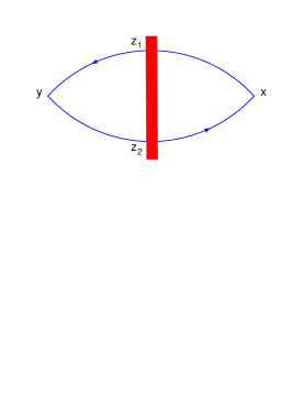
Figure 1: Diagram for the LO impact factor. We indicate in blue the quantum fields and in red the classical background ones.

4 Numerical parameters

In this section we provide the numerical values of the parameters that will be used in the subsequent sections.

As initial condition for the evolution of the Ioffe-time distribution, the pseudo-PDF and quasi-PDF, we will use the GBW model which has an $x_{B}$ dependence of the saturation scale as $Q_{s}=\left(x_{0}/x_{B}\right)^{0.277\over 2}$, with $x_{0}=0.41\times 10^{-4}$  Golec-Biernat:1998js . The dimension of the dipole cross-section is given by the parameter $\sigma_{0}=29.12$ mb Golec-Biernat:1998js . Our starting point for the evolution in $x_{B}$ will be $x_{B}=0.1$ for which $Q_{s}=0.34$ GeV. As we will see, $x_{B}=0.1$ is the point at which the BFKL logarithms start to be of order $1$ thus need to be resummed. However, the conclusions we will reach through our analysis will not depend on the starting point of the evolution.

The value of the running coupling we choose is $\bar{\alpha}_{s}={\alpha_{s}N_{c}\over\pi}=0.2$. Since at low-$x_{B}$ the strong coupling runs with the transverse size of the dipole Balitsky:2006wa ; Kovchegov:2006vj ; Balitsky:2007feb , our choice of the running coupling corresponds to a transverse size of about $0.2\,{\rm GeV}^{-1}$ so that the running-coupling is evaluated at a momentum scale greater than our choice of $Q_{s}$.

As we will show in subsequent sections, there is a correspondence between the Ioffe-time $z\cdot P$ and the $x_{B}$ of the type $z\cdot P=x_{B}^{-1}$. So, to calculate the large longitudinal distance behavior of the Ioffe-time distribution, we use as starting point of the evolution (in the Ioffe-time parameter) the value $\varrho\equiv z\cdot P=10$ and we fix $|z|=0.5\,{\rm GeV}^{-1}$.

For the quasi-PDF, we introduce the unit vector $\xi^{\mu}$ in the direction of the gauge link and choose the projection of the target momentum $P$ along $\xi^{\mu}$ to be $\xi\cdot P\equiv P_{\xi}=4$ GeV (see section 8 for details).

5 Ioffe-time gluon distribution at large longitudinal distances

In this section we are going to calculate the behavior of Ioffe-time gluon distribution at large longitudinal distances in the saddle point approximation. We will show that large distance, i.e. large values of the Ioffe-time $z\cdot P=\varrho$, generates large logarithms which are resummed by the BFKL equation through the HE-OPE formalism. Therefore, we will refer to high-energy or large-distance behavior interchangeably.

As discussed in the previous section, the Ioffe-time gluon distribution is defined by

$$\langle{P}|{G^{a}}^{i-}(z)[z,0]{G^{b}_{i}}^{-}(0)|{P}\rangle=2(P^{-})^{2}{\cal M}_{pp}(\varrho,z^{2})\,.$$ (14)

In the high-energy (Regge) limit forward matrix elements of $U_{x}U^{\dagger}_{y}$ operator are divergent because they contain an unrestricted integration along the $n^{\mu}$ direction, so we have

$$2\pi\delta(\epsilon^{-})\langle{P}|G^{a\,i-}(x^{+},x_{\perp})[nx^{+}+x_{\perp},0]^{ab}G_{i}^{b\,-}(0)|{P}\rangle$$

$$~{}~{}=\int_{-\infty}^{+\infty}\!dy^{+}\langle{P}|G^{a\,i-}(x^{+}+y^{+},x_{\perp})$$

$$\times[n(x^{+}+y^{+})+x_{\perp},ny^{+}]^{ab}G_{i}^{b\,-}(y^{+})|{P+\epsilon^{-}n}\rangle\,.$$ (15)

As described in section 3, the first step is to calculate the impact factor from the operator (15). To this end, we split all fields in quantum and classical, functionally integrate over the quantum field and obtain the diagram in figure 2.

Assuming that the shock-wave is in $x^{+}=0$ position, we distinguish the cases $x^{+}>0>y^{+}$ and $x^{+}<0<y^{+}$. The high-energy gluon propagator at $x^{+}>0>y^{+}$ in coordinate space Balitsky:2009yp is

$$\langle{\rm T}A_{\mu}^{a}(x)A^{b}_{\nu}(y)\rangle\stackrel{{\scriptstyle x^{+}>0>y^{+}}}{{=}}$$

$$-{1\over 4\pi^{3}}\int d^{2}z\,U^{ab}_{z}{x^{+}|y^{+}|g^{\perp}_{\mu\nu}-|y^{+}|n^{\prime}_{\mu}X^{\perp}_{\nu}+x^{+}n^{\prime}_{\nu}Y^{\perp}_{\mu}+n^{\prime}_{\mu}n^{\prime}_{\nu}(X,Y)\over\Big{[}2(x-y)^{-}x^{+}|y^{+}|-|y^{+}|(x-z)^{2}_{\perp}-x^{+}(y-z)^{2}_{\perp}+i\epsilon\Big{]}^{2}}\,,$$ (16)

where we defined $X_{2\perp}=(x-z_{2})_{\perp}$ and $Y_{2\perp}=(y-z_{2})_{\perp}$.

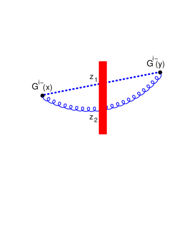
Figure 2: Diagrams for the impact factors for the quasi-PDFs operators. The black bullets represent the gluons and quark fields respectively.

So, using propagator (16) diagram 2 is

$$\langle G^{a\,i-}(x^{+},x_{\perp})[nx^{+}+x_{\perp},ny^{+}+y_{\perp}]^{ab}G^{b\,j-}(y^{+},y_{\perp})\rangle_{{\rm Fig.}\ref{Fig:quasipdf-gq-LO}}$$

$$\stackrel{{\scriptstyle y^{+}<0<x^{+}}}{{=}}(\partial_{x}^{i}g^{\mu-}-\partial_{x}^{-}g^{i\mu})(\partial_{y}^{j}g^{\nu-}-\partial_{y}^{-}g^{j\nu})\langle A^{a}_{\mu}(x)A^{b}_{\nu}(y)\rangle_{A}$$

$$=-\!\int{d^{2}z_{2}\over 4\pi^{3}}\,U^{ab}_{z_{2}}U^{ab}_{z_{1}}\,(\partial_{x}^{i}g^{\mu-}-\partial_{x}^{-}g^{i\mu})(\partial_{y}^{j}g^{\nu-}-\partial_{y}^{-}g^{j\nu})$$

$$~{}~{}~{}\times{x^{+}|y^{+}|g^{\perp}_{\mu\nu}-|y^{+}|n^{\prime}_{\mu}X^{\perp}_{2\nu}+x^{+}n^{\prime}_{\nu}Y^{\perp}_{2\mu}+n^{\prime}_{\mu}n^{\prime}_{\nu}(X_{2},Y_{2})\over\Big{[}|y^{+}|(x-z_{2})^{2}_{\perp}+x^{+}(y-z_{2})^{2}_{\perp}-i\epsilon\Big{]}^{2}}\,.$$ (17)

Result (17) is proportional to two Wilson lines in the adjoint representation, one at point $z_{2\perp}$ as a result of the gluon propagation in the shock-wave external field, and the other one at point $z_{1\perp}$ which is the point at which the shock-wave intersects the gauge link $[nx^{+}+x_{\perp},ny^{+}+y_{\perp}]^{ab}$. The point $z_{1}$ can actually be anywhere between point $nx^{+}+x_{\perp}$ and $ny^{+}+y_{\perp}$, so we parametrize the straight line between these two points as $x_{u}=ux_{\perp}+{\bar{u}}y_{\perp}=z_{1\perp}$, with $u={|y^{+}|\over\Delta^{+}}$, ${\bar{u}}={x^{+}\over\Delta^{+}}$ and $\Delta^{+}=x^{+}-y^{+}$, and at the end we will have to integrate over the parameter $u$. However, for technical reason, as it will be clear later, we will continue to call such point as $z_{1\perp}$.

After differentiation, eq. (17) becomes

$$\langle G^{a\,i-}(x^{+},x_{\perp})[nx^{+}+x_{\perp},ny^{+}+y_{\perp}]^{ab}G_{i}^{b\,-}(y^{+},y_{\perp})\rangle_{{\rm Fig.}\ref{Fig:quasipdf-gq-LO}}$$

$$~{}~{}\stackrel{{\scriptstyle y^{+}<0<x^{+}}}{{=}}\!\!\int{d^{2}z_{2}\over 4\pi^{3}}\Bigg{[}12\,{-2x^{+}y^{+}(x-z_{2},y-z_{2})^{2}+x^{+}y^{+}(x-z_{2})^{2}_{\perp}(y-z_{2})^{2}_{\perp}\over\big{[}x^{+}(y-z_{2})^{2}_{\perp}-y^{+}(x-z_{2})^{2}_{\perp}\big{]}^{4}}\Bigg{]}U^{ab}_{z_{2}}U^{ab}_{z_{1}}\,,$$ (18)

As done for the photon impact factor in section 3, we include the case $\theta(x^{+}y^{+})$ and consider forward matrix elements. Thus, we make the substitution $U^{ab}_{z_{2}}U^{ab}_{z_{1}}$ with $-2N^{2}_{c}{\cal U}(z_{12})$ where ${\cal U}(z_{12})=1-{1\over N_{c}}{\rm tr}\{U_{z_{1\perp}}U^{\dagger}_{z_{2\perp}}\}$ and ${\rm tr}$ trace in the fundamental representation.

Let us observe that we have put the starting operator in the left-hand-side of eq. (17) in the form of impact factor convoluted with matrix element of Wilson lines as it was in the case of the T-product of two electromagnetic current in eq. (7). The last step of the high-energy OPE is to convolute the impact factor with the solution of the evolution equation of the Wilson-line operators, eq. (13). So, we have

$$g_{ij}\langle G^{a\,i-}(x^{+},x_{\perp})[nx^{+}+x_{\perp},ny^{+}+y_{\perp}]^{ab}G^{b\,j-}(y^{+},y_{\perp})\rangle_{{\rm Fig.}\ref{Fig:quasipdf-gq-LO}}$$

$$~{}~{}\stackrel{{\scriptstyle y^{+}<0<x^{+}}}{{=}}-{6N^{2}_{c}\over(x^{+}|y^{+}|)^{3}}\int{d\nu\over 2\pi^{2}}\,\left(-{2{\Delta^{+}}^{2}u{\bar{u}}\over\Delta^{2}_{\perp}}{{P^{-}}^{2}\over M^{2}_{N}}+i\epsilon\right)^{{\alpha_{s}N_{c}\over 2\pi}\chi(\nu)}\int d^{2}\omega(\omega^{2}_{\perp})^{-{1\over 2}-i\nu}\langle{\cal V}^{a_{0}}(\omega_{\perp})\rangle$$

$$~{}~{}~{}~{}~{}~{}\times\!\int{d^{2}z_{2}\over\pi^{3}}\,{-2(x-z_{2},y-z_{2})^{2}_{\perp}+(x-z_{2})^{2}_{\perp}(y-z_{2})^{2}_{\perp}\over\left({(y-z_{2})^{2}_{\perp}\over|y^{+}|}+{(x-z_{2})^{2}_{\perp}\over x^{+}}\right)^{4}}(z_{12}^{2})^{{1\over 2}+i\nu}\,.$$ (19)

In section A we show that the matrix element in eq. (19) with transverse indexes $i$ and $j$ not contracted, after projection on the power like eigenfunction $(z_{12}^{2})^{{1\over 2}+i\nu}$, has only one tensor structure, that is $g^{ij}$.

Here, we proceed with contracted $i$ and $j$ indexes, and obtain

$$\int{d^{2}z_{2}\over\pi^{3}}\,{-2(x-z_{2},y-z_{2})^{2}_{\perp}+(x-z_{2})^{2}_{\perp}(y-z_{2})^{2}_{\perp}\over\left({(y-z_{2})^{2}_{\perp}\over|y^{+}|}+{(x-z_{2})^{2}_{\perp}\over x^{+}}\right)^{4}}(z_{12}^{2})^{{1\over 2}+i\nu}$$

$$=-{\gamma^{2}\over\pi^{2}}(\Delta^{+})^{4}(\Delta^{2}_{\perp})^{\gamma-1}\Gamma(1-\gamma)\Gamma(1+\gamma)(u{\bar{u}})^{\gamma+3}\,.$$ (20)

Using (20) in (19) and integrating over $u$ we arrive at

$$\int_{-\infty}^{+\infty}\!\!\!dx^{+}dy^{+}\!\,\delta(x^{+}-y^{+}-L)\langle G^{a\,i-}(x^{+},x_{\perp})[nx^{+}+x_{\perp},ny^{+}+y_{\perp}]^{ab}G_{i}^{b\,-}(y^{+},y_{\perp})\rangle_{{\rm Fig.}\ref{Fig:quasipdf-gq-LO}}$$

$$=6N^{2}_{c}\int{d\nu\over 2\pi^{2}}\left(-{2u{\bar{u}}\over\Delta^{2}_{\perp}}{(LP^{-})^{2}\over M^{2}_{N}}+i\epsilon\right)^{{\alpha_{s}N_{c}\over 2\pi}\chi(\nu)}\int d^{2}\omega(\omega^{2}_{\perp})^{-{1\over 2}-i\nu}\langle{\cal V}^{a_{0}}(\omega_{\perp})\rangle$$

$$~{}~{}~{}\times\!\!\int_{0}^{1}\!{du\over L}{\gamma^{2}\over\pi^{2}}(\Delta^{2}_{\perp})^{\gamma-1}\Gamma(1-\gamma)\Gamma(1+\gamma)(u{\bar{u}})^{\gamma}$$

$$=3N^{2}_{c}\int\!d\nu\left(-{2(LP^{-})^{2}\over\Delta^{2}_{\perp}M^{2}_{N}}+i\epsilon\right)^{{\aleph(\gamma)\over 2}}{(\Delta^{2}_{\perp})^{\gamma-1}\over L\,\pi^{4}}{\pi\gamma\over\sin\pi\gamma}{\gamma^{4}\Gamma^{2}(\gamma)\over\Gamma(2+2\gamma)}$$

$$~{}~{}~{}\times\!\!\int d^{2}\omega(\omega^{2}_{\perp})^{-{1\over 2}-i\nu}\langle{\cal V}^{a_{0}}_{\omega}\rangle+{\cal O}(\alpha_{s})\,.$$ (21)

We will evaluate the integration over the parameter $\nu$ numerically and compare it with the saddle point approximation. The GBW model Golec-Biernat:1998js applied to the Wilson-line dipole matrix element evaluated in the target nucleon state is (see figure 3).

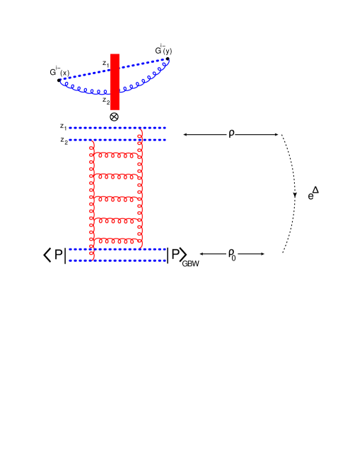
Figure 3: Diagrammatic representation of the HE-OPE applied to the gluon non-local operator with “quasi-PDF frame”.

$$\langle{P}|{\cal U}(x-y)|{P+\epsilon^{-}n^{\prime}}\rangle= P^{-}2\pi\delta(\epsilon^{-})\langle\langle{P}|{\cal U}(x-y)_{\perp}|{P}\rangle\rangle$$

$$= P^{-}2\pi\delta(\epsilon^{-})\sigma_{0}\left(1-\exp\Big{(}{-(x-y)^{2}_{\perp}Q^{2}_{s}\over 4}\Big{)}\right)\,,$$ (22)

where, as discussed in section 4, the saturation scale assume the fixed value of $Q_{s}=0.34$ GeV.

So, using (22) in eq. (21) we arrive, with the help of eq. (15), at

$${1\over 2(P^{-})^{2}}\langle{P}|G^{a\,i-}(L,x_{\perp})[nL+x_{\perp},0]^{ab}G_{i}^{b\,-}(0)|{P}\rangle$$

$$={3N^{2}_{c}\over 2\pi^{3}}{\sigma_{0}\over\Delta^{2}_{\perp}}{1\over LP^{-}}\!\int\!d\nu\left(-{2(LP^{-})^{2}\over\Delta^{2}_{\perp}M^{2}_{N}}+i\epsilon\right)^{\aleph(\gamma)\over 2}{\gamma\,\Gamma^{2}(1-\gamma)\Gamma^{3}(1+\gamma)\over\Gamma(2+2\gamma)}\left({Q^{2}_{s}\Delta^{2}_{\perp}\over 4}\right)^{\gamma}\,.$$ (23)

Let $z^{\mu}$ be a space-like vector. In the high-energy limit, the coordinate $x^{+}$ component is enhanced, the $x^{-}$ one is suppressed, and the $x_{\perp}$ component is left invariant, so $|\Delta_{\perp}|=\sqrt{-z^{2}}=|z|>0$ with $z^{2}<0$. Since at this regime we do not distinguish between the $0$ and the $3$-component, we also have $(P^{-})^{2}=(P\cdot{z\over|z|})^{2}={\varrho^{2}\over-z^{2}}$ and $LP^{-}\to z\cdot P=\varrho$. Using variables $\varrho$ and $z^{2}$, and eq. (2) with $z^{2}\neq 0$, result (23) becomes

$${\cal M}_{pp}(\varrho,z^{2})={3N^{2}_{c}\over 4\pi^{3}}{Q_{s}\sigma_{0}\over|z|\varrho}\!\int\!d\nu\!\left({2\,\varrho^{2}\over z^{2}M^{2}_{N}}+i\epsilon\right)^{\aleph(\gamma)\over 2}{\gamma\,\Gamma^{2}(1-\gamma)\Gamma^{3}(1+\gamma)\over\Gamma(2+2\gamma)}\left({|z|Q_{s}\over 2}\right)^{\!2i\nu}\,.$$ (24)

We are now ready to perform last integration using the saddle-point approximation technique. We notice that ${\gamma\Gamma^{2}(1-\gamma)\Gamma^{3}(1+\gamma)\over\Gamma(2+2\gamma)}$, is a very slowly varying function, so we have

$${\cal M}_{pp}(\varrho,z^{2})\simeq{3N^{2}_{c}\over 128\,\varrho}{Q_{s}\,\sigma_{0}\over|z|}\left({2\,\varrho^{2}\over z^{2}M^{2}_{N}}+i\epsilon\right)^{\bar{\alpha}_{s}2\ln 2}{e^{-{\ln^{2}{Q_{s}|z|\over 2}\over 7\zeta(3)\bar{\alpha}_{s}\ln\left({2\,\varrho^{2}\over z^{2}M^{2}_{N}}+i\epsilon\right)}}\over\sqrt{7\zeta(3)\bar{\alpha}_{s}\ln\left({2\,\varrho^{2}\over z^{2}M^{2}_{N}}+i\epsilon\right)}}\,.$$ (25)

Figure 4: In the left and in the right panel we plot the numerical evaluation of real and imaginary part of (24) (orange curve), and the real and imaginary part of the saddle point result (25) (blue dashed curve), respectively.

In figure 4 we compare the saddle-point result (25) with the numerical integration (24).

The first thing to notice is that, the logarithms resummed by BFKL are $\bar{\alpha}_{s}\ln\left({\sqrt{2}\varrho\over|z|M_{M}}\right)$ which, given that we are using $\bar{\alpha}_{s}=0.2$, $|z|=0.5\,{\rm GeV}^{-1}$, and $M_{N}=1$ GeV, is of order 1 starting from $\varrho\sim 10$. We see that $\varrho$ acts like a rapidity parameter. We evolve the distribution with $\varrho$ until $\bar{\alpha}_{s}\ln\left({\sqrt{2}\varrho\over|z|M_{M}}\right)$ is of order $1$, that is we start with large values of $\varrho$ and end at smaller ones. The dipole at the smallest value of $\varrho$ is evaluated in the GBW model. In our case, as anticipated in section 4, we stop the evolution at $\varrho=10$ (see figure 3).

In Fig. 4 we plotted the real and imaginary part of (24) and (25) with $\varrho\in[10,400]$. For the subsequent analysis we will use the numerical evaluation of (24) (orange curve).

6 Leading and Next-to-leading Twist

As described in section 3, within the high-energy OPE, the DIS cross section can be written as a convolution of the impact factor and the solution of the evolution equation of the matrix elements of the dipole-Wilson-line operator which, in the linear case, is the BFKL equation. Therefore, the dipole DIS cross-section can be written as

$$\sigma^{\gamma^{*}p}(x_{B},Q^{2})=\int d\nu\,F(\nu)\,x_{B}^{-\aleph(\nu)-1}\left({Q^{2}\over P^{2}}\right)^{{1\over 2}+i\nu}\,,$$ (26)

where $\aleph(\gamma)$ is the BFKL pomeron intercept, $F(\nu)$ the pomeron residue, and in the limit under consideration, $-q^{2}=Q^{2}\gg P^{2}$, and $s=(P+q)^{2}\gg Q^{2}$.

To get the dipole cross-section given in eq. (26) we can calculate the integral over the $\nu$-parameter numerically, or with the saddle point approximation capturing in this way the full BFKL dynamics. In the previous section, we have done this for the gluon Ioffe-time distribution (see eqs. (24) and (25)).

The $n$-th moment of the structure function is

$$M_{n}=\int_{0}^{1}dx_{B}\,x_{B}^{n-1}\sigma^{\gamma^{*}p}(x_{B},Q^{2})=\int_{{1\over 2}-i\infty}^{{1\over 2}+i\infty}d\gamma\,{F(\gamma)\over n-1-\aleph(\gamma)}\left({Q^{2}\over P^{2}}\right)^{\gamma}\,,$$

where $\gamma={1\over 2}+i\nu$. The integration over the $\gamma$-parameter can be performed closing the contour to the left of the poles. In this way we get the anomalous dimensions of the leading and higher twist operators at the unphysical point.

In our case, to get the LT and NLT contributions from the infinite series of twists, resummed by BFKL eq., we could repeat the same steps outlined above. However, this time we need the explicit form of the gluon twist-two operator at the unphysical point $n=1$, $F^{a}_{\mu_{+}}\nabla^{-1}_{+}F^{\mu a}_{+}$.

In Ref. BALITSKY:2014zza (see also Balitsky:2013npa ; Balitsky:2018irv ) it was shown that the analytical continuation of anomalous dimension of twist-two gluon operator ${\cal O}^{j}_{F}\equiv F_{\mu}^{a\,-}\nabla_{+}^{j-2}F^{a\,\mu-}$ to the unphysical point $j=1$, which is determined by BFKL equation, can be obtained by the analytic continuation of the operator itself at such unphysical point. It is known that the anomalous dimensions are singular at $j=1$, and this means that in this limit there is a different hierarchy of perturbation theory which requires a new resummation of terms like $\left({\alpha_{s}\over j-1}\right)^{n}$ (at leading-log), and therefore it implies the existence of a different (than DGLAP) evolution equation, the BFKL equation, which resums such logarithms. For this reason we will refer to the Regge limit also as the $j\to 1$ limit. The relation between DGLAP and BFKL equation at the unphysical point was established, at the level of anomalous dimension, at LO in Ref Jaroszewicz:1982gr and at NLO in Ref. Fadin:1998py .

In Ref. Balitsky:1987bk it was shown that the local Operator Product Expansion can be reformulated in terms of non-local operators with the advantage of preserving explicitly the Lorentz and the conformal invariance of the theory and also providing a gauge covariant technique to separating higher twist contribution. Such non-local operator are light-ray operator with integration over the longitudinal direction. In light of this, in Ref. BALITSKY:2014zza , it is shown how to construct analytic continuation of non-local operator at $j=1$. Following the procedure described in Ref. Balitsky:2018irv , in section B, we will show that such analytic continuation of local operator is

$$F_{p_{1}\xi}^{a}(x)\nabla^{j-2}F_{p_{1}}^{a~{}\xi}(x)\Big{|}_{x=0}\stackrel{{\scriptstyle\rm forw.}}{{=}}{1\over\Gamma(2-j)}\int^{\infty}_{0}dv\,v^{1-j}\,F^{a}_{p_{1}\xi}(0)[0,vp_{1}]^{ab}F^{b~{}\xi}_{p_{1}}(vp_{1})\,,$$ (27)

where $p_{1}$ is a light-cone vector and where the notation $x_{p_{1}}=p_{1}^{\mu}x_{\mu}$ has been used (see section B for the details). Equation (27) is the gluon light-ray operator with spin $j$.

It turns out that in the high-energy (Regge) limit the correlation function of two gluon light-ray operators (27), with spin $j$ and $j^{\prime}$ respectively, are UV divergent if taken on the light-cone. In Refs. Balitsky:2013npa ; Balitsky:2015tca ; Balitsky:2015oux ; Balitsky:2018irv it was shown that a way to regularize this UV divergence is to consider the point-splitting regulator, that is, the light-ray operator, which lays on the light-cone, becomes a rectangular frame, the “Wilson-frame” (see figure 12). In section B we will show that an alternative regulator is the “quasi-pdf frame” (see figure 12) defined as

$${\cal F}^{j}(x,y)=\int_{0}^{+\infty}du^{1-j}\,{F^{a\,i}}_{p_{1}}(up_{1}+x)[up_{1}+x,y]^{ab}{F_{i}^{b\,}}_{p_{1}}(y)\,.$$ (28)

As a consistency check, we will also show that, in the high-energy regime correlation functions of two such operators, eq. (28), agrees with the expected result from conformal field theory.

The Mellin transform of eq. (23), which is, as explained above, the analytic continuation to non integer $j$ of local operator with “quasi-pdf frame” is

$$\int_{\Delta^{2}_{\perp}M_{N}}^{+\infty}\!dL\,L^{1-j}\int_{-\infty}^{+\infty}\!dy^{+}\langle{P}|G^{a\,i-}(L+y^{+},x_{\perp})$$

$$~{}~{}~{}~{}~{}~{}~{}~{}~{}~{}~{}~{}~{}~{}~{}~{}~{}~{}~{}~{}~{}~{}~{}~{}~{}\times[n(L+y^{+})+x_{\perp},ny^{+}+y_{\perp}]^{ab}G_{i}^{b\,-}(y^{+},y_{\perp})|{P}\rangle$$

$$=-{3\,i\,N^{2}_{c}\sigma_{0}P^{-}\over\pi^{3}\Delta^{2}_{\perp}}\int_{{1\over 2}-i\infty}^{{1\over 2}+i\infty}\!d\gamma\,{\theta(\Re[j-1-\aleph(\gamma)])\over\omega-\aleph(\gamma)}{\gamma\Gamma^{2}(1-\gamma)\Gamma^{3}(1+\gamma)\over\Gamma(2+2\gamma)}\left({Q^{2}_{s}\Delta^{2}_{\perp}\over 4}\right)^{\gamma}$$

$$~{}~{}\times\!\left(-{2{P^{-}}^{2}\over\Delta^{2}_{\perp}M^{2}_{N}}+i\epsilon\right)^{\aleph(\gamma)\over 2}(\Delta^{2}_{\perp}P^{-})^{-\omega+\aleph(\gamma)}\,,$$ (29)

with $\omega=j-1$, and where we required that the longitudinal distance (in $x^{+}$ direction) $L\geq\Delta^{2}_{\perp}M_{N}$ that is equivalent to say that our hypothetical probe has a power resolution smaller than the hadron size i.e. that we are in the perturbative regime.

Closing the contour to the right of $\gamma={1\over 2}$, we can now take the residue at the point $\gamma^{*}$ such that $\aleph(\gamma^{*})-\omega=0$ we have

$$\int_{\Delta^{2}_{\perp}M_{N}}^{+\infty}\!dL\,L^{1-j}\int_{-\infty}^{+\infty}\!dy^{+}\langle{P}|G^{a\,i-}(L+y^{+},x_{\perp})$$

$$~{}~{}~{}~{}~{}~{}~{}~{}~{}~{}~{}~{}~{}~{}~{}~{}~{}~{}~{}~{}~{}~{}~{}~{}~{}\times[n(L+y^{+})+x_{\perp},ny^{+}+y_{\perp}]^{ab}G_{i}^{b\,-}(y^{+},y_{\perp})|{P}\rangle$$

$$={6\,N^{2}_{c}\over\pi^{2}}{\Delta^{-2}_{\perp}\sigma_{0}P^{-}\over\aleph^{\prime}(\gamma^{*})}{\gamma^{*}\Gamma^{2}(1-\gamma^{*})\Gamma^{3}(1+\gamma^{*})\over\Gamma(2+2\gamma^{*})}\left({Q^{2}_{s}\Delta^{2}_{\perp}\over 4}\right)^{\gamma^{*}}\left({2{P^{-}}^{2}\over\Delta^{2}_{\perp}M^{2}_{N}}\right)^{\omega\over 2}\,.$$ (30)

So far, the calculation was done in the “BFKL” limit in which ${\bar{\alpha}_{s}\over j-1}\simeq 1$. To get the leading and next-to-leading residues in power of $Q^{2}_{s}\Delta^{2}_{\perp}$ we need to approach the “DGLAP” limit by assuming the $\bar{\alpha}_{s}\ll\omega\ll 1$. In this limit, then, we can use $\omega-\aleph(\gamma)\to\omega-{\bar{\alpha}_{s}\over 1-\gamma}$ and the leading residue is at $\gamma=1-{\bar{\alpha}_{s}\over\omega}$. Thus, from eq. (30) we obtain

$$\int_{\Delta^{2}_{\perp}M_{N}}^{+\infty}\!dL\,L^{1-j}\int_{-\infty}^{+\infty}\!dy^{+}{1\over 2P^{-}}\langle{P}|G^{a\,i-}(L+y^{+},x_{\perp})$$

$$~{}~{}~{}~{}~{}~{}~{}~{}~{}~{}~{}~{}~{}~{}~{}~{}~{}~{}~{}~{}~{}~{}~{}~{}~{}\times\![n(L+y^{+})+x_{\perp},ny^{+}+y_{\perp}]^{ab}G_{i}^{b\,-}(y^{+},y_{\perp})|{P}\rangle$$

$$={3\,N^{2}_{c}Q^{2}_{s}\sigma_{0}\over 4\pi^{2}}\left({Q^{2}_{s}\Delta^{2}_{\perp}\over 4}\right)^{-{\bar{\alpha}_{s}\over\omega}}\left(-{2{P^{-}}^{2}\over\Delta^{2}_{\perp}M^{2}_{N}}+i\epsilon\right)^{\omega\over 2}g_{1}(\omega)\,,$$ (31)

where we have defined the function $g_{1}(\omega)$ as

$$g_{1}(\omega)\equiv{\bar{\alpha}_{s}\over\omega^{2}}{(1-{\bar{\alpha}_{s}\over\omega})\Gamma^{2}({\bar{\alpha}_{s}\over\omega})\Gamma^{3}(2-{\bar{\alpha}_{s}\over\omega})\over\Gamma(4-2{\bar{\alpha}_{s}\over\omega})}\,.$$ (32)

The first thing to notice is that we have recovered the gluon anomalous dimension ${\bar{\alpha}_{s}\over j-1}$ in the $j\to 1$ limit as anticipated above. Moreover, the leading residue is leading in terms of $Q_{s}^{2}\Delta_{\perp}^{2}$ expansion, so eq. (31) is the leading twist contribution.

Similarly, we can calculate the next-to-leading residue in power of $\left({Q_{s}^{2}\Delta_{\perp}^{2}\over 4}\right)^{\!2}$. We start again from eq. (30) and using $\omega-\aleph(\gamma)\to\omega-{\bar{\alpha}_{s}\over 2-\gamma}$, the next-to-leading residue is at $\gamma=2-{\bar{\alpha}_{s}\over\omega}$

$$\int_{\Delta^{2}_{\perp}M_{N}}^{+\infty}\!dL\,L^{1-j}\int_{-\infty}^{+\infty}\!dy^{+}{1\over 2P^{-}}\langle{P}|G^{a\,i-}(L+y^{+},x_{\perp})$$

$$~{}~{}~{}~{}~{}~{}~{}~{}~{}~{}~{}~{}~{}~{}~{}~{}~{}~{}~{}~{}~{}~{}~{}~{}~{}\times[n(L+y^{+})+x_{\perp},ny^{+}+y_{\perp}]^{ab}G_{i}^{b\,-}(y^{+},y_{\perp})|{P}\rangle$$

$$\ni{3\,N^{2}_{c}Q^{2}_{s}\sigma_{0}\over 4\pi^{2}}{Q^{2}_{s}\Delta^{2}_{\perp}\over 4}\left({Q^{2}_{s}\Delta^{2}_{\perp}\over 4}\right)^{-{\bar{\alpha}_{s}\over\omega}}\left(-{2{P^{-}}^{2}\over\Delta^{2}_{\perp}M^{2}_{N}}+i\epsilon\right)^{\!{\omega\over 2}}g_{2}(\omega)\,,$$ (33)

where we have defined the function $g_{2}(\omega)$ as

$$g_{2}(\omega)\equiv{\bar{\alpha}_{s}\over\omega^{2}}{(2-{\bar{\alpha}_{s}\over\omega})\Gamma^{2}({\bar{\alpha}_{s}\over\omega}-1)\Gamma^{3}(3-{\bar{\alpha}_{s}\over\omega})\over\Gamma(6-2{\bar{\alpha}_{s}\over\omega})}\,.$$ (34)

We see that the next-to-leading residue, eq. (33), in the limit of small distances $\Delta^{2}_{\perp}$, is suppressed by one power of $Q^{2}_{s}\Delta^{2}_{\perp}\over 4$ respect to the leading residue contribution (31).

We can continue in this way and calculate the full series of twist expansion which is resummed in eq. (23) or from its saddle approximation, eq. (25). However, one has to notice that, besides the residues which give the twist expansion, in eq. (29) there is another pole, the one at $\gamma=1$. This pole, actually, cancel out with two diagrams that are not included in the high-energy OPE and that have to be calculated separately. To see how this cancellation happen, one can consider the correlation of two light-ray operator at high-energy with “quasi-pdf” point splitting regulator (see section B for details). In this way, we may be sure that our procedure is justified.

Adding together the leading residue, eq. (31), and the next-to-leading residue, eq. (33), we obtain

$$\int_{\Delta^{2}_{\perp}M_{N}}^{+\infty}\!dL\,L^{1-j}\int_{-\infty}^{+\infty}\!dy^{+}{1\over 2P^{-}}\langle{P}|G^{a\,i-}(L+y^{+},x_{\perp})$$

$$~{}~{}~{}~{}~{}~{}~{}~{}~{}~{}~{}~{}~{}~{}~{}~{}~{}~{}~{}~{}~{}~{}~{}~{}~{}\times\![n(L+y^{+})+x_{\perp},ny^{+}+y_{\perp}]^{ab}G_{i}^{b\,-}(y^{+},y_{\perp})|{P}\rangle$$

$$={3\,N^{2}_{c}Q^{2}_{s}\sigma_{0}\over 4\pi^{2}}\left({4\over Q^{2}_{s}\Delta^{2}_{\perp}}\right)^{{\bar{\alpha}_{s}\over\omega}}\left(-{2{P^{-}}^{2}\over\Delta^{2}_{\perp}M^{2}_{N}}+i\epsilon\right)^{\omega\over 2}\left(g_{1}(\omega)+g_{2}(\omega){Q^{2}_{s}\Delta^{2}_{\perp}\over 4}\right)\,.$$ (35)

The final step is to perform the inverse Mellin transform of (35)

$$\int_{-\infty}^{+\infty}\!dy^{+}{1\over 2P^{-}}\langle{P}|G^{a\,i-}(L+y^{+},x_{\perp})$$

$$~{}~{}~{}~{}~{}~{}~{}~{}~{}~{}~{}~{}~{}~{}~{}~{}~{}~{}~{}~{}~{}~{}~{}~{}~{}\times\![n(L+y^{+})+x_{\perp},ny^{+}+y_{\perp}]^{ab}G_{i}^{b\,-}(y^{+},y_{\perp})|{P}\rangle\theta(L-\Delta^{2}_{\perp}M_{N})$$

$$={3\,N^{2}_{c}Q^{2}_{s}\sigma_{0}\over 4\pi^{2}}{1\over 2\pi i}\int_{1-i\infty}^{1+i\infty}d\omega L^{\omega-1}\left({4\over Q^{2}_{s}\Delta^{2}_{\perp}}\right)^{{\bar{\alpha}_{s}\over\omega}}\left(-{2{P^{-}}^{2}\over\Delta^{2}_{\perp}M^{2}_{N}}+i\epsilon\right)^{\omega\over 2}$$

$$~{}~{}\times\!\left(g_{1}(\omega)+g_{2}(\omega){Q^{2}_{s}\Delta^{2}_{\perp}\over 4}\right)\,.$$ (36)

Using variables $\varrho$ and $z^{2}$, and eq. (2) with $z^{2}\neq 0$, we can rewrite eq. (36) as

$${\cal M}_{pp}(\varrho,z^{2})=\!\!\! {3\,N^{2}_{c}\over 4\pi^{2}}{Q^{2}_{s}\sigma_{0}\over\varrho}{1\over 2\pi i}\int_{1-i\infty}^{1+i\infty}d\omega\!\left({4\over Q^{2}_{s}|z|^{2}}\right)^{{\bar{\alpha}_{s}\over\omega}}\left({2\,\varrho^{2}\over z^{2}M^{2}_{N}}+i\epsilon\right)^{\omega\over 2}$$ (37)

$$\times\!\left(g_{1}(\omega)+g_{2}(\omega){Q^{2}_{s}|z|^{2}\over 4}\right)\,.$$

Result (37) is our final result which gives the behavior of the LT and NLT gluon distribution at high-energy in coordinate space and from which we will calculate the pseudo and quasi-PDFs at LT and NLT corrections

In the limit $\bar{\alpha}_{s}\ll\omega\ll 1$, we have

$$g_{1}(\omega)\simeq{1\over 6\bar{\alpha}_{s}}\,,~{}~{}~{}~{}~{}~{}g_{2}(\omega)\simeq{2\over 15\bar{\alpha}_{s}}\,.$$ (38)

So, using approximations (38), eq. (37) becomes

$${\cal M}_{pp}(\varrho,z^{2})=\!\!\! {N^{2}_{c}\over 8\pi^{2}}{Q^{2}_{s}\sigma_{0}\over\bar{\alpha}_{s}\varrho}{1\over 2\pi i}\int_{1-i\infty}^{1+i\infty}\!d\omega\left({4\over Q^{2}_{s}|z|^{2}}\right)^{{\bar{\alpha}_{s}\over\omega}}\left({2\,\varrho^{2}\over z^{2}M^{2}_{N}}+i\epsilon\right)^{\!{\omega\over 2}}$$ (39)

$$\times\!\left(1+{Q^{2}_{s}|z|^{2}\over 5}\right)+O\!\left({Q^{4}_{s}|z|^{4}\over 16}\right)\,.$$

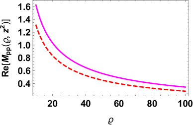
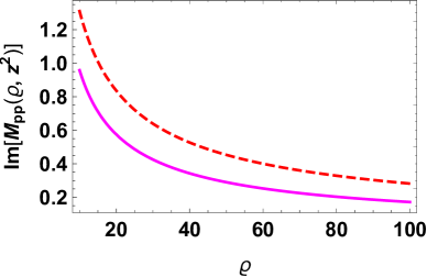
Figure 5: In the left and right panel we plot the real and imaginary part of eq. (37) (red dashed curve), and the real and imaginary part of eq. (42) (magenta curve), respectively.

From eq. (39) we can perform the inverse Mellin analytically. We have to distinguish two cases. In the first case, ${Q^{2}_{s}|z|^{2}\over 4}>1$, the twist expansion is not justified and all order corrections will have to be included. Indeed, if we perform the inverse Mellin transform we get

$${\cal M}_{pp}(\varrho,z^{2})=\!\!\! -{N^{2}_{c}\over 8\pi^{2}\bar{\alpha}_{s}}{Q^{2}_{s}\sigma_{0}\over\varrho}\left({2\bar{\alpha}_{s}\ln{Q^{2}_{s}|z|^{2}\over 4}\over\ln\!\left({2\,\varrho^{2}\over z^{2}M_{N}^{2}}+i\epsilon\right)}\right)^{\!\!\!{1\over 2}}\!\!\!J_{1}(t)\left(1+{Q^{2}_{s}|z|^{2}\over 5}\right)+O\!\left({Q^{4}_{s}|z|^{4}\over 16}\right)\,,$$ (40)

with

$$t=\left[2\bar{\alpha}_{s}\ln\left({Q^{2}_{s}|z|^{2}\over 4}\right)\ln\!\left({2\varrho^{2}\over z^{2}M_{N}^{2}}+i\epsilon\right)\right]^{1\over 2}\,,$$ (41)

and where, we recall, $z^{2}<0$. Result (40) gives an unusual behavior as a remnant of the fact that case ${Q^{2}_{s}|z|^{2}\over 4}>1$ is not justified in terms of twist expansion.

For the second case $0<{Q^{2}_{s}|z|^{2}\over 4}<1$, which corresponds to the typical DIS region, the twist expansion is justified. In this case we obtain

$${\cal M}_{pp}(\varrho,z^{2})={N^{2}_{c}\over 8\pi^{2}\bar{\alpha}_{s}}{Q^{2}_{s}\sigma_{0}\over\varrho}\left({4\bar{\alpha}_{s}\left|\ln{Q_{s}|z|\over 2}\right|\over\ln\!\left({2\,\varrho^{2}\over z^{2}M_{N}^{2}}+i\epsilon\right)}\right)^{\!\!\!{1\over 2}}\!\!\!I_{1}(\tilde{t})\left(1+{Q^{2}_{s}|z|^{2}\over 5}\right)+O\!\left({Q^{4}_{s}|z|^{4}\over 16}\right)\,,$$ (42)

with

$$\tilde{t}=\left[4\bar{\alpha}_{s}\left|\ln{Q_{s}|z|\over 2}\right|\ln\!\left({2\,\varrho^{2}\over z^{2}M_{N}^{2}}+i\epsilon\right)\right]^{1\over 2}\,.$$ (43)

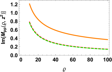
Figure 6: In the left panel, the orange curve is the numerical evaluation of real part of eq. (24) (all twist resummed by BFKL), the green dashed curve is the real part of the LT term in (37) only, while the red dashed one is the real part of LT+NLT result, eq. (37). In the left panel we plot the imaginary parts. The range of $\varrho$ is from $10$ to $100$.

The goodness of approximation (38) can be appreciated in Fig. 5 where we plot result (37) with inverse Mellin is performed numerically with $0<{Q^{2}_{s}|z|\over 4}<1$, and result (42).

In Fig. 6 we finally compare the coordinate space result of the high-energy (large $\varrho$) behavior of the gluon distribution with BFKL resummation, eq. (24), the LT term and LT plus NLT of eq. (37). We notice that the curves plotted in figure 6 are very slowly varying functions for large values of $\varrho$ (see figure 7).

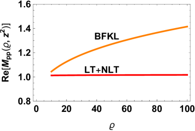
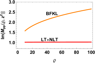
Figure 7: Here we plot the real and imaginary part of the BFKL (23) and LT+NLT (37) both normalized to the LT, respectively; $\varrho$ variates from $10$ to $100$.

Moreover, as mentioned in the previous section, the region of applicability of our formalism is where the BFKL logarithm $\bar{\alpha}_{s}\ln\left({\sqrt{2}\varrho\over|z|M_{N}}\right)$ is of order 1 which is for $\varrho\geq 10$.

7 Gluon pseudo-PDF

The pseudo-PDF Radyushkin:2017cyf are defined as the Fourier transform of the matrix element of the gluon bi-local operator with respect to the momentum $P^{\mu}$ keeping its orientation fixed. In our notation this translates into the Fourier transform of eq. (24) and eq. (37) with respect to $\varrho$.

7.1 Gluon pseudo-PDF with BFKL resummation

We defined the pseudo-PDF in eq. (5), so we have to perform the Fourier transform of eq. (24) with respect to $\varrho$

$$G_{\rm p}(x_{B},z^{2})=\!\!\! {3N_{c}^{2}\over 4\pi^{3}}{Q_{s}\sigma_{0}\over|z|}\int\!\!{d\varrho\over 2\pi\varrho}e^{-i\varrho x_{B}}\!\!\int\!d\nu\left({2\varrho^{2}\over z^{2}M_{N}^{2}}+i\epsilon\right)^{\!\!\aleph(\gamma)\over 2}$$ (44)

$$\times\!{\gamma\,\Gamma^{2}(1-\gamma)\Gamma^{3}(1+\gamma)\over\Gamma(2+2\gamma)}\left({|z|Q^{2}_{s}\over 2}\right)^{\!\!2i\nu}\,.$$

It is convenient to performing first the Fourier transform and the integration over the $\nu$ parameter at the end. So, we have

$$G_{\rm p}(x_{B},z^{2})=\!\!\! -i{3N^{2}_{c}\over 4\pi^{4}}{Q_{s}\sigma_{0}\over|z|}\int\!d\nu\left({2\over x_{B}^{2}z^{2}M^{2}_{N}}+i\epsilon\right)^{\!\!\aleph(\gamma)\over 2}\left({Q_{s}|z|\over 2}\right)^{2i\nu}$$ (45)

$$\times{\gamma\,\Gamma^{2}(1-\gamma)\Gamma^{3}(1+\gamma)\Gamma(\aleph(\gamma))\over\Gamma(2+2\gamma)}\sin\left({\pi\over 2}\aleph(\gamma)\right){\rm sign}(x_{B})\,.$$

Evaluating the last integration in the saddle-point approximation we have

$$G_{\rm p}(x_{B},z^{2}) \simeq-i{3N^{2}_{c}\over 128\pi}{Q_{s}\sigma_{0}\over|z|}{\Gamma(\bar{\alpha}_{s}4\ln 2)\sin({\pi\over 2}\bar{\alpha}_{s}4\ln 2)\over\sqrt{7\zeta(3)\bar{\alpha}_{s}\ln\left({2\over x_{B}^{2}z^{2}M^{2}_{N}}+i\epsilon\right)}}{\rm sign}(x_{B})$$ (46)

$$~{}\times\!\exp\!\left\{{-\ln^{2}{Q_{s}|z|\over 2}\over 7\zeta(3)\bar{\alpha}_{s}\ln\left({2\over x_{B}^{2}z^{2}M^{2}_{N}}+i\epsilon\right)}\right\}\left({2\over x_{B}^{2}z^{2}M^{2}_{N}}+i\epsilon\right)^{\bar{\alpha}_{s}2\ln 2}\,.$$

Note that, in eq. (46) we can further approximate $\Gamma(\bar{\alpha}_{s}4\ln 2)\sin({\pi\over 2}\bar{\alpha}_{s}4\ln 2)\simeq{\pi\over 2}$ for small values of $\bar{\alpha}_{s}$.

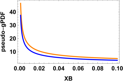
Figure 8: The orange curve is the numerical integration of the real part of (45), while the blue one is the saddle-point approximation (46)(real part).

As can be observed in Fig. 8, the numerical evaluation of result (45) is very well approximated by the saddle-point approximation result (46).

7.2 Gluon pseudo-PDF at LT and NLT

Let us perform the Fourier transform to obtain the pseudo-PDF for the leading and next-to-leading twist corrections. Our starting point is the Fourier transform of eq. (37) which, using the pseudo-PDF definition eq. (5), is

$$G_{\rm p}(x_{B},z^{2})=\!\!\! {3N^{2}_{c}\,Q^{2}_{s}\sigma_{0}\over 16\pi^{2}}{1\over 2\pi i}\int_{1-i\infty}^{1+i\infty}d\omega\int_{0}^{+\infty}\!\!{d\varrho\over 2\pi\varrho}\,e^{-i\varrho x_{B}}$$ (47)

$$\times\!\left({2\varrho^{2}\over z^{2}M_{N}^{2}}+i\epsilon\right)^{\!\!{\omega\over 2}}\left({4\over Q^{2}_{s}|z|^{2}}\right)^{\!\!{\bar{\alpha}_{s}\over\omega}}\Big{(}4g_{1}(\omega)+g_{2}(\omega)Q_{s}^{2}|z|^{2}\Big{)}+O\!\left({Q_{s}^{4}|z|^{4}\over 16}\right)\,.$$

From eq. (47) we will first perform the Fourier transform and lastly the inverse Mellin transform. Thus, we have

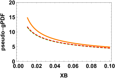
Figure 9: In the left panel we plot pseudo-PDF with BFKL resummation, eq. (45) (orange curve), and the LT (green dashed curve) and LT+NLT (red dashed curve) of pseudo-PDF result (48); The value of $x_{B}$ is between 0.001 to 0.02. In the right panel we plot the same curves in a different range of $x_{B}$ between 0.01 to 0.1.

$$G_{\rm p}(x_{B},z^{2})=\!\!\! {3N^{2}_{c}\,Q^{2}_{s}\sigma_{0}\over 32\pi^{3}}{1\over 2\pi i}\int_{1-i\infty}^{1+i\infty}d\omega\,\left({2\over x_{B}^{2}|z|^{2}M_{N}^{2}}\right)^{\omega\over 2}\left({4\over Q^{2}_{s}|z|^{2}}\right)^{{\bar{\alpha}_{s}\over\omega}}\Gamma(\omega)$$ (48)

$$\times\left(4g_{1}(\omega)+g_{2}(\omega)Q_{s}^{2}|z|^{2}\right)+O\!\left({Q_{s}^{4}|z|^{4}\over 16}\right)\,.$$

The LT and NLT result, eq. (48), is obtained in the limit $\bar{\alpha}_{s}\ll\omega\ll 1$, so, we could further approximate eq. (48) using eq. (38) and also approximating $\Gamma(\omega)\stackrel{{\scriptstyle\omega\to 0}}{{\simeq}}{1\over\omega}$ and obtain

$$G_{\rm p}(x_{B},z^{2})=\!\!\! {N^{2}_{c}\,Q^{2}_{s}\sigma_{0}\over 16\bar{\alpha}_{s}\pi^{3}}{1\over 2\pi i}\int_{1-i\infty}^{1+i\infty}{d\omega\over\omega}\,\left({2\over x_{B}^{2}|z|^{2}M_{N}^{2}}\right)^{\omega\over 2}\left({4\over Q^{2}_{s}|z|^{2}}\right)^{{\bar{\alpha}_{s}\over\omega}}$$ (49)

$$\times\left(1+{Q_{s}^{2}|z|^{2}\over 5}\right)+O\!\left({Q_{s}^{4}|z|^{4}\over 16}\right)\,.$$

In appendix D we will employ such approximations, perform the inverse Mellin transform obtaining an analytic expression, and compare the result with the numerical evaluation of eq. (48), thus showing the goodness of the approximated analytic result. However, for our analysis, we will consider the numerical evaluation of eq. (48).

In Fig. 9, we plot the gluon pseudo-PDF with the BFKL resummation eq. (46) (orange curve), and the LT term and the LT plus NLT of eq. (48) (green dashed and red dashed curve respectively). We observe that the BFKL resummation result agrees with the LT and LT+NLT result in the region of moderate $x_{B}$. When we move into the low-$x_{B}$ region, we notice a strong disagreement which confirms the necessity of a $\ln{1\over x_{B}}$ resummation represented by BFKL eq.

8 Gluon quasi-PDF

To obtain the quasi-PDF, we need to perform again a Fourier transform of eq. (24) which, this time, takes a slightly different form then the pseudo-PDF case considered in the previous section. Let us introduce the real parameter $\varsigma$ such that $-z^{2}=\varsigma^{2}>0$, and the four-vector $\xi^{\mu}\equiv{z^{\mu}\over|z|}={z^{\mu}\over|\varsigma|}$ with $|z|=\sqrt{-z^{2}}$. The quasi-PDF are defined as the Fourier transform of the coordinate space gluon distributions (24) and (37) keeping, this time, the orientation of the vector $z^{\mu}$ fixed.

8.1 Gluon quasi-PDF with BFKL resummation

Let us start with eq. (24). As already mentioned before, in the high-energy limit, where $x^{+}$-component $\to\infty$ and $x^{-}$-component $\to 0$, we can not distinguish between the zeroth and the third component. We can then rewrite $LP^{-}=z\cdot P=\varsigma P_{\xi}$ with $P_{\xi}\equiv P\cdot\xi=P^{-}$ because the $\xi^{\mu}$ vector, in the limit we are considering, selects the minus component of the $P^{\mu}$ vector. Moreover, in coordinate space, in the high-energy limit, every fields depends only on $x^{+}$ and $x_{\perp}$, so, restoring the $x^{-}$ components amounts in substituting $(x-y)^{2}_{\perp}=\Delta^{2}_{\perp}\to-z^{2}=\varsigma^{2}$. In the quasi-PDF notation eq. (23) becomes

$${\xi_{\mu}\xi_{\nu}\over 2P_{\xi}^{2}}\langle{P}|G^{a\,\alpha\mu}(\varsigma)[\varsigma,0]^{ab}G_{\alpha}^{b\,\nu}(0)|{P}\rangle$$

$$=\,{3N^{2}_{c}\over 4\pi^{3}}{Q_{s}\sigma_{0}\over\varsigma^{2}P_{\xi}}\int\!d\nu\,\left(-{2P^{2}_{\xi}\over M^{2}_{N}}+i\epsilon\right)^{\aleph(\gamma)\over 2}{\gamma\,\Gamma^{2}(1-\gamma)\Gamma^{3}(1+\gamma)\over\Gamma(2+2\gamma)}\left({Q^{2}_{s}\varsigma^{2}\over 4}\right)^{i\nu}\,.$$ (50)

We can then use the definition of the gluon quasi-PDF eq. (6)

$$G_{\rm q}(x_{B},P_{\xi})=\!\!\! P_{\xi}\int{d\varsigma\over 2\pi}\,e^{-i\varsigma P_{\xi}x_{B}}{\xi_{\mu}\xi_{\nu}\over 2P_{\xi}^{2}}\langle{P}|G^{a\,\alpha\mu}(\varsigma)[\varsigma,0]^{ab}G_{\alpha}^{b\,\nu}(0)|{P}\rangle$$

$$=\!\!\! {3N^{2}_{c}\over 8\pi^{4}}Q_{s}\sigma_{0}\int\!d\nu\,\left(-{2P^{2}_{\xi}\over M^{2}_{N}}+i\epsilon\right)^{\aleph(\gamma)\over 2}{\gamma\,\Gamma^{2}(1-\gamma)\Gamma^{3}(1+\gamma)\over\Gamma(2+2\gamma)}$$ (51)

$$\times\!\int\!{d\varsigma\over\varsigma^{2}}\left({Q^{2}_{s}\varsigma^{2}\over 4}\right)^{i\nu}\!e^{-i\varsigma P_{\xi}x_{B}}\,.$$

Performing the integration over $\varsigma$ we obtain (recall that we are using $\gamma={1\over 2}+i\nu$)

$$G_{\rm q}(x_{B},P_{\xi})=\!\!\! i\,{3N^{2}_{c}\over 4\pi^{4}}Q_{s}\sigma_{0}P_{\xi}|x_{B}|\int\!d\nu\left(\!-{2P^{2}_{\xi}\over M^{2}_{N}}+i\epsilon\right)^{\!\!\aleph(\gamma)\over 2}\!\!\left(Q^{2}_{s}\over 4P_{\xi}^{2}x_{B}^{2}\right)^{\!\!i\nu}$$ (52)

$$\times\!{\gamma\,\Gamma^{2}(1-\gamma)\Gamma^{3}(1+\gamma)\Gamma(2\gamma-2)\over\Gamma(2+2\gamma)}\sinh(\pi\nu)\,.$$

Let us calculate eq. (52) in the saddle point approximation. To this end we note that ${\gamma\,\Gamma^{2}(1-\gamma)\Gamma^{3}(1+\gamma)\Gamma(2\gamma-2)\over\Gamma(2+2\gamma)}\sinh(\pi\nu)$ is a slowly varying function, so in the saddle point approximation we have

$$G_{\rm q}(x_{B},P_{\xi})\simeq\!\!\! -{3N^{2}_{c}\over 256}Q_{s}\sigma_{0}P_{\xi}|x_{B}|\left(-{2P^{2}_{\xi}\over M^{2}_{N}}+i\epsilon\right)^{\bar{\alpha}_{s}2\ln 2}\!\!{e^{-{\ln^{2}{Q_{s}\over 2P_{\xi}|x_{B}|}\over 7\bar{\alpha}_{s}\zeta(3)\ln\left(-{2P^{2}_{\xi}\over M^{2}_{N}}+i\epsilon\right)}}\over\sqrt{7\zeta(3)\bar{\alpha}_{s}\ln\left(-{2P^{2}_{\xi}\over M^{2}_{N}}+i\epsilon\right)}}\,.$$ (53)

In Fig. 10 we compare eqs. (53) with its saddle point approximation result (53) calculated with a large values of $P_{\xi}$.

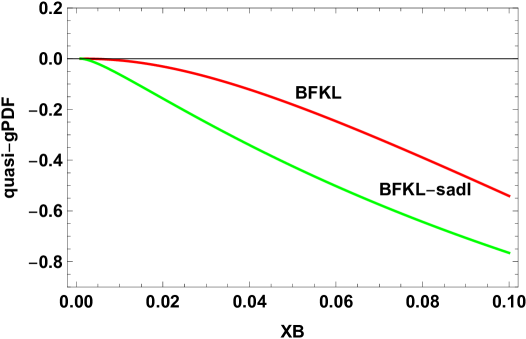
Figure 10: Here we compare eq. (52) (real part) with its saddle point approximation, (53) (real part). The curves are plotted in the range $x_{B}\in[0.001,0.1]$ with $P_{\xi}=4$ GeV.

It is interesting to notice that, in the gluon quasi-PDF case, the usual exponentiation of the pomeron intercept (the LO BFKL eigenvalues $\aleph(\gamma)$), which indicates the resummation of large logarithms of ${1\over x_{B}}$, is absent. The exponentiation of the pomeron intercept that we instead have in eq. (52) (and also in (53)) suggests that the logarithms resummed by BFKL equation are $\alpha_{s}\ln\left({2P_{\xi}^{2}\over M^{2}_{N}}\right)$ rather than the usual $\alpha_{s}\ln{1\over x_{B}}$ as in the pseudo-PDF case (see equations (45) and (46)).

8.2 Gluon quasi-PDF at LT and NLT

Let us now consider the leading and next-to-leading twist gluon quasi-PDF. We have to perform the quasi-PDF Fourier transform of eq. (36) and make the inverse Mellin transform at the end. So, using the quasi-PDF variables $\varsigma$ and $P_{\xi}$, we have

$$G_{\rm q}(x_{B},P_{\xi})$$

$$=\!\!\! P_{\xi}\int{d\varsigma\over 2\pi}\,e^{-i\varsigma P_{\xi}x_{B}}{\xi_{\mu}\xi_{\nu}\over 2P_{\xi}^{2}}\langle{P}|G^{a\,\alpha\mu}(\varsigma)[\varsigma,0]^{ab}G_{\alpha}^{b\,\nu}(0)|{P}\rangle$$

$$=\!\!\! P_{\xi}\int_{0}^{+\infty}{d\varsigma\over 2\pi}\,e^{-i\varsigma P_{\xi}x_{B}}{3N^{2}_{c}\,Q^{2}_{s}\,\sigma_{0}\over 16\pi^{2}}{1\over 2\pi i}\int_{1-i\infty}^{1+i\infty}\,{d\omega\over\varsigma P_{\xi}}\left(-{2P_{\xi}^{2}\over M_{N}^{2}}+i\epsilon\right)^{\omega\over 2}\left({4\over Q^{2}_{s}\varsigma^{2}}\right)^{{\bar{\alpha}_{s}\over\omega}}$$ (54)

$$\times\!\Big{(}4g_{1}(\omega)+g_{2}(\omega)Q^{2}_{s}\varsigma^{2}\Big{)}\,.$$

Performing the integration over $\varsigma$ we get

$$G_{\rm q}(x_{B},P_{\xi})=\!\!\! {3N^{2}_{c}\,Q^{2}_{s}\,\sigma_{0}\over 32\pi^{3}}{1\over 2\pi i}\int_{1-i\infty}^{1+i\infty}\!\!d\omega\left(-{2P_{\xi}^{2}\over M_{N}^{2}}+i\epsilon\right)^{\!\!{\omega\over 2}}\left(-{4P_{\xi}^{2}x_{B}^{2}\over Q^{2}_{s}}+i\epsilon\right)^{\!\!{\bar{\alpha}_{s}\over\omega}}$$ (55)

$$\times\Gamma\!\left(-{2\bar{\alpha}_{s}\over\omega}\right)\left(4\,g_{1}(\omega)+{2\bar{\alpha}_{s}\over\omega}{Q^{2}_{s}\over P_{\xi}^{2}x_{B}^{2}}\left(1-{2\bar{\alpha}_{s}\over\omega}\right)g_{2}(\omega)\right)\,.$$

Equation (55) is the gluon quasi-PDF up to next-to-leading twist contribution. What one should notice in result (55) is the strong enhancement of the NLT term with respect to the LT term due to the ${1\over P_{\xi}^{2}x_{B}^{2}}$ factor. This is also consistent with the result obtained in Ref. Braun:2018brg .

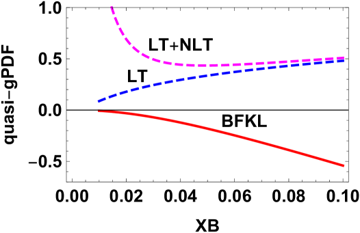
Figure 11: Here we plot the quasi-PDF with BFKL rsummation eq. (52) (real part), the LT and the LT+NLT of eq. (55) (real part). The curves are plotted in the range $x_{B}\in[0.01,0.1]$ with $P_{\xi}=4$ GeV.

Since we are in the approximation $\bar{\alpha}_{s}\ll\omega\ll 1$, employing equations $(\ref{g1g2approxy})$, and $\Gamma\left(-{2\bar{\alpha}_{s}\over\omega}\right)\simeq-{\omega\over 2\bar{\alpha}_{s}}$, we can also simplify result (55) as

$$G_{\rm q}(x_{B},P_{\xi})=\!\!\! -{N^{2}_{c}\,Q^{2}_{s}\,\sigma_{0}\over 16\bar{\alpha}_{s}^{2}\pi^{3}}{1\over 2\pi i}\int_{1-i\infty}^{1+i\infty}\!\!d\omega\left(-{2P_{\xi}^{2}\over M_{N}^{2}}+i\epsilon\right)^{\!\!{\omega\over 2}}\left(-{4P_{\xi}^{2}x_{B}^{2}\over Q^{2}_{s}}+i\epsilon\right)^{\!\!{\bar{\alpha}_{s}\over\omega}}$$ (56)

$$\times\left(\omega+{2\bar{\alpha}_{s}Q_{s}^{2}\over 5P_{\xi}^{2}x_{B}^{2}}+O\left({\bar{\alpha}_{s}\over\omega}\right)\right)\,.$$

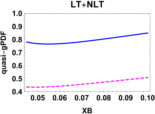
Figure 16: Here, we compare the real part of eq. (55) (magenta-dashed curve) with its approximation, real part of eq. (123) (blue curve). This time we are in the case $\ln{4P_{\xi}^{2}x_{B}^{2}\over Q^{2}_{s}}>0$, with $P_{\xi}=4$ GeV, and $x_{B}\in[0.045,0.1]$.

In appendix E we provide the analytic expression of eq. (56) in two different cases: $\ln{4P_{\xi}^{2}x_{B}^{2}\over Q^{2}_{s}}>0$ and $\ln{4P_{\xi}^{2}x_{B}^{2}\over Q^{2}_{s}}<0$ and compare them with result (55) (see figures. 15 and 16). However, although our conclusions are not affected by using either of the results (56), or (55), in what follow we will plot the numerical evaluation of eq. (55).

In Fig. 11, using $P_{\xi}=4$ GeV, we plot the quasi-PDF with BFKL resummation (red curve) given in eq. (52), and the LT (blue dashed curve), and LT+NLT (magenta dashed curve) contributions given in eq. (55). What is striking about the plot in Fig. 11 is that the behavior of the three curves is different than the usual low-$x_{B}$ behavior of gluon distributions which we, instead, observed for the pseudo-PDF distribution in Fig. 9. We considered again as initial condition of the evolution the GBW model evaluated at $x_{B}=0.1$. One may check that, changing the starting point of the evolution, for example evaluating the GBW model at $x_{B}=0.01$, would not change such unusual behavior of the quasi-PDF.

9 Conclusions

Our findings are illustrated in figures 6, 9, and 11 where we plotted the Ioffe-time distributions, the pseudo-PDF and quasi-PDF respectively.

The main result is that the pseudo-PDF and the quasi-PDF have a very different behavior at low-$x_{B}$. The physical origin of the difference between the two distributions lay in the two different Fourier transforms under which they are defined. More precisely, in the pseudo-PDF case, the scale is the resolution that is, the square of the length of the gauge link separating the bi-local operator. On the other hand, in the quasi-PDF case, the scale is the energy that is, the momentum of the hadronic target (the nucleon) projected along the direction of the gauge link. Indeed, if on one hand, the pseudo-PDF has the typical behavior of the gluon distribution at low-$x_{B}$ (see figure 9), on the other hand, the quasi-PDF has a rather unusual low-$x_{B}$ behavior (see figure 11). The reason is that the usual exponentiation of the BFKL pomeron intercept, which resums logarithms of $x_{B}$, is absent in the quasi-PDF result (52). Moreover, the power corrections in the quasi-PDF result (55) do not come in as inverse powers of $P$ but as inverse powers of $x_{B}P$, so for low values of $x_{B}$ and fixed values of $P$ these corrections are enhanced rather than suppressed at this regime.

Another result we obtained is the large-distance behavior of the gluon Ioffe-time distribution (see figure 6) where we noticed that the plotted curves (for the real and imaginary part) are very slowly varying functions for large values of $\varrho$ (see figure 7). Indeed, since in lattice calculations the values of $\varrho$ is not very large, to perform the Fourier transform and obtain the $x_{B}$ dependence, one has to extrapolate the large-distance behavior of the Ioffe-time distribution.

In this work, running coupling corrections and next-to-leading order BFKL have not been used and could be included. Moreover, the technique we developed in this work can be extended to study the low-$x_{B}$ behavior of other unpolarized or polarized pseudo and quasi parton distributions.

The author is grateful to I. Balitsky and V. Braun for valuable discussions. He also thanks A. Manashov and A. Vladimirov for discussions.

Appendix A Projection with open transverse indexes

He we consider the gluon matrix element with open transverse indexes. We start from

$$\langle G^{a\,i-}(x^{+},x_{\perp})[nx^{+}+x_{\perp},ny^{+}+y_{\perp}]^{ab}G^{b\,j-}(y^{+},y_{\perp})\rangle_{{\rm Fig.}\ref{Fig:quasipdf-gq-LO}}$$

$$=(\partial_{x}^{i}g^{\mu-}-\partial_{x}^{-}g^{i\mu})(\partial_{y}^{j}g^{\nu-}-\partial_{y}^{-}g^{j\nu})\langle A^{a}_{\mu}(x)A^{b}_{\nu}(y)\rangle_{A}\,.$$ (57)

Using the gluon propagator (16) in (57) we get

$$\langle G^{a\,i-}(x^{+},x_{\perp})[nx^{+}+x_{\perp},ny^{+}+y_{\perp}]^{ab}G^{b\,j-}(y^{+},y_{\perp})\rangle_{{\rm Fig.}\ref{Fig:quasipdf-gq-LO}}$$

$$=(\partial_{x}^{-}g^{i\mu}-\partial_{x}^{i}g^{\mu-})(\partial_{y}^{j}g^{\nu-}-\partial_{y}^{-}g^{j\nu})$$

$$\times\!\int{d^{2}z_{2}\over 4\pi^{3}}\,{x^{+}|y^{+}|g^{\perp}_{\mu\nu}-|y^{+}|n^{\prime}_{\mu}X^{\perp}_{2\nu}+x^{+}n^{\prime}_{\nu}Y^{\perp}_{2\mu}+n^{\prime}_{\mu}n_{2\nu}(X_{2},Y_{2})\over\Big{[}|y^{+}|(x-z_{2})^{2}_{\perp}+x^{+}(y-z_{2})^{2}_{\perp}-i\epsilon\Big{]}^{2}}\,U^{ab}_{z_{2}}U^{ab}_{z_{1}}\,.$$ (58)

After differentiation eq. (58) becomes

$$\langle G^{a\,i-}(x^{+},x_{\perp})[nx^{+}+x_{\perp},ny^{+}+y_{\perp}]^{ab}G^{b\,j-}(y^{+},y_{\perp})\rangle_{{\rm Fig.}\ref{Fig:quasipdf-gq-LO}}$$

$$=\int{d^{2}z_{2}\over 4\pi^{3}}\Bigg{\{}{4\,g^{ij}\over[x^{+}(y-z_{2})^{2}_{\perp}-y^{+}(x-z_{2})^{2}_{\perp}]^{2}}$$

$$+{4y^{+}g^{ij}(x-z_{2})^{2}_{\perp}-4x^{+}g^{ij}(y-z_{2})^{2}_{\perp}-12y^{+}(x-z_{2})^{i}(x-z_{2})^{j}+12x^{+}(y-z_{2})^{i}(y-z_{2})^{j}\over[x^{+}(y-z_{2})^{2}_{\perp}-y^{+}(x-z_{2})^{2}_{\perp}]^{3}}$$

$$+{1\over[x^{+}(y-z_{2})^{2}_{\perp}-y^{+}(x-z_{2})^{2}_{\perp}]^{4}}\Big{(}24x^{+}y^{+}(x-z_{2},y-z_{2})(x-z_{2})^{i}(y-z_{2})^{j}$$

$$-12{y^{+}}^{2}(x-z_{2})^{2}_{\perp}(x-z_{2})^{i}(x-z_{2})^{j}-12{x^{+}}^{2}(y-z_{2})^{2}_{\perp}(y-z_{2})^{i}(y-z_{2})^{j}$$

$$-6g^{ij}x^{+}y^{+}(x-z_{2})^{2}_{\perp}(y-z_{2})^{2}_{\perp}\Big{)}\Bigg{\}}U^{ab}_{z_{2}}U^{ab}_{z_{1}}\,.$$ (59)

We recall that the point $z_{1}$ can be anywhere between point $nx^{+}+x_{\perp}$ and $ny^{+}+y_{\perp}$. We parametrize the straight line between these two points as $x_{u}=ux_{\perp}+{\bar{u}}y_{\perp}=z_{1\perp}$, with $u={|y^{+}|\over\Delta^{+}}$, ${\bar{u}}={x^{+}\over\Delta^{+}}$ and $\Delta^{+}=x^{+}-y^{+}$, and at the end we will have to integrate over the parameter $u$.

Considering forward matrix elements and including the solution of the linear evolution of the Wilson-line operator (BFKL equation)

$${\cal V}^{a}(z_{12})=\!\!\int{d\nu\over 2\pi^{2}}\,(z_{12}^{2})^{-{1\over 2}+i\nu}\left(-{2x^{+}y^{+}\over(x-y)^{2}a_{0}}+i\epsilon\right)^{{\alpha_{s}N_{c}\over 2\pi}\chi(\gamma)}\!\!\int d^{2}\omega(\omega^{2}_{\perp})^{-{1\over 2}-i\nu}{\cal V}^{a_{0}}(\omega_{\perp})$$ (60)

with ${1\over z_{12}^{2}}{\cal U}^{a}(z_{12})={\cal V}^{a}(z_{12})$, $\aleph(\gamma)=\bar{\alpha}_{s}\chi(\gamma)$, $\gamma={1\over 2}+i\nu$, and $\chi(\gamma)=2\psi(1)-\psi(\gamma)-\psi(1-\gamma)$, from (59) we arrive at

$$\langle G^{a\,i-}(x^{+},x_{\perp})[nx^{+}+x_{\perp},ny^{+}+y_{\perp}]^{ab}G^{b\,j-}(y^{+},y_{\perp})\rangle_{{\rm Fig.}\ref{Fig:quasipdf-gq-LO}}$$

$$=\int{d^{2}z_{2}\over 4\pi^{3}}\Bigg{\{}{4\,g^{ij}\over[x^{+}(y-z_{2})^{2}_{\perp}-y^{+}(x-z_{2})^{2}_{\perp}]^{2}}$$

$$~{}~{}+{4y^{+}g^{ij}(x-z_{2})^{2}_{\perp}-4x^{+}g^{ij}(y-z_{2})^{2}_{\perp}-12y^{+}(x-z_{2})^{i}(x-z_{2})^{j}+12x^{+}(y-z_{2})^{i}(y-z_{2})^{j}\over[x^{+}(y-z_{2})^{2}_{\perp}-y^{+}(x-z_{2})^{2}_{\perp}]^{3}}$$

$$~{}~{}+{1\over[x^{+}(y-z_{2})^{2}_{\perp}-y^{+}(x-z_{2})^{2}_{\perp}]^{4}}\Big{(}24x^{+}y^{+}(x-z_{2},y-z_{2})(x-z_{2})^{i}(y-z_{2})^{j}$$

$$~{}~{}-12{y^{+}}^{2}(x-z_{2})^{2}_{\perp}(x-z_{2})^{i}(x-z_{2})^{j}-12{x^{+}}^{2}(y-z_{2})^{2}_{\perp}(y-z_{2})^{i}(y-z_{2})^{j}$$

$$~{}~{}-6g^{ij}x^{+}y^{+}(x-z_{2})^{2}_{\perp}(y-z_{2})^{2}_{\perp}\Big{)}\Bigg{\}}$$

$$~{}~{}\times\!z_{12}^{2}\int{d\nu\over 2\pi^{2}}\,(z_{12}^{2})^{-{1\over 2}+i\nu}\left(-{2x^{+}y^{+}\over(x-y)^{2}a_{0}}+i\epsilon\right)^{{\alpha_{s}N_{c}\over 2\pi}\chi(\gamma)}\int d^{2}\omega(\omega^{2}_{\perp})^{-{1\over 2}-i\nu}{\cal V}^{a_{0}}(\omega_{\perp})\,.$$ (61)

The projection over the open indexes tensor structure is

$$\int{d^{2}z_{2}\over 4\pi^{3}}\Bigg{\{}{4\,g^{ij}\over[x^{+}(y-z_{2})^{2}_{\perp}-y^{+}(x-z_{2})^{2}_{\perp}]^{2}}$$

$$+{4y^{+}g^{ij}(x-z_{2})^{2}_{\perp}-4x^{+}g^{ij}(y-z_{2})^{2}_{\perp}-12y^{+}(x-z_{2})^{i}(x-z_{2})^{j}+12x^{+}(y-z_{2})^{i}(y-z_{2})^{j}\over[x^{+}(y-z_{2})^{2}_{\perp}-y^{+}(x-z_{2})^{2}_{\perp}]^{3}}$$

$$+{1\over[x^{+}(y-z_{2})^{2}_{\perp}-y^{+}(x-z_{2})^{2}_{\perp}]^{4}}\Big{(}24x^{+}y^{+}(x-z_{2},y-z_{2})(x-z_{2})^{i}(y-z_{2})^{j}$$

$$-12{y^{+}}^{2}(x-z_{2})^{2}_{\perp}(x-z_{2})^{i}(x-z_{2})^{j}-12{x^{+}}^{2}(y-z_{2})^{2}_{\perp}(y-z_{2})^{i}(y-z_{2})^{j}$$

$$-6g^{ij}x^{+}y^{+}(x-z_{2})^{2}_{\perp}(y-z_{2})^{2}_{\perp}\Big{)}\Bigg{\}}(z^{2}_{12})^{\gamma}$$

$$=g^{ij}{3\over 2}{\gamma^{2}\Gamma(1+\gamma)\Gamma(1-\gamma)\over\pi^{2}{\Delta^{+}}^{2}}{(u{\bar{u}})^{\gamma}\over[\Delta^{2}_{\perp}]^{1-\gamma}}\,,$$ (62)

with $\Delta_{\perp}^{2}=(x-y)^{2}_{\perp}=-(x-y)^{i}(x-y)_{i}$. We see that only one tensor structure survived after projection. So, using result (62) in eq. (61) we obtain

$${\cal V}^{a}(z_{12})=\int{d\nu\over 2\pi^{2}}\,(z_{12}^{2})^{-{1\over 2}+i\nu}\left(-{2x^{+}y^{+}\over(x-y)^{2}a_{0}}+i\epsilon\right)^{{\alpha_{s}N_{c}\over 2\pi}\chi(\gamma)}\!\!\int d^{2}\omega(\omega^{2}_{\perp})^{-{1\over 2}-i\nu}{\cal V}^{a_{0}}(\omega_{\perp})\,,$$ (63)

with ${1\over z_{12}^{2}}{\cal U}^{a}(z_{12})={\cal V}^{a}(z_{12})$, $\aleph(\gamma)=\bar{\alpha}_{s}\chi(\gamma)$, $\gamma={1\over 2}+i\nu$, and $\chi(\gamma)=2\psi(1)-\psi(\gamma)-\psi(1-\gamma)$, from (59) we arrive at

$$\langle G^{a\,i-}(x^{+},x_{\perp})[nx^{+}+x_{\perp},ny^{+}+y_{\perp}]^{ab}G^{b\,j-}(y^{+},y_{\perp})\rangle_{{\rm Fig.}\ref{Fig:quasipdf-gq-LO}}$$

$$=\int{d\nu\over 2\pi^{2}}\left(-{2x^{+}y^{+}\over(x-y)^{2}a_{0}}+i\epsilon\right)^{{\alpha_{s}N_{c}\over 2\pi}\chi(\gamma)}\int d^{2}\omega(\omega^{2}_{\perp})^{-{1\over 2}-i\nu}{\cal V}^{a_{0}}(\omega_{\perp})$$

$$~{}\times g^{ij}{3\over 2}{\gamma^{2}\Gamma(1+\gamma)\Gamma(1-\gamma)\over\pi^{2}{\Delta^{+}}^{2}}{(u{\bar{u}})^{\gamma}\over[\Delta^{2}_{\perp}]^{1-\gamma}}\,.$$ (64)

Integrating over $u$ and contracting the transverse indexes $i$ and $j$, from (64) we arrive at result (21).

Appendix B From local operators to Light-ray operators

It is known that correlation functions of non-local operators on the light-cone are UV divergent in the high-energy (Regge) limit and that a way to regulate these divergences is to consider the point-splitting regulator. In this section we will first show that the “quasi-pdf frame” (see figure 12) is a valid point-splitting regulator for correlation function of non-local operators at high-energy (Regge) limit, and that, in this limit, it gives the same result as the one obtained in Refs. Balitsky:2015oux ; Balitsky:2018irv using the “Wilson-frame” (see figure 12). In this way we can show that diagrams a) and b) of figure 13 which are not included in the HE-OPE formalism do not contribute. This is because these diagrams cancel out with the residue at $\gamma=1$ as explained in section 6.

In this section we will also use light-cone vectors $p_{1}$ and $p_{2}$ such that $2p_{1}\cdot p_{2}=s$, and $x_{p_{1}}=p_{1}^{\mu}x_{\mu}=\sqrt{s/2}\,x^{-}$, and $x_{p_{2}}=p_{2}^{\mu}x_{\mu}=\sqrt{s/2}\,x^{+}$. The light cone vectors $n^{\mu}$ and $n^{\prime\mu}$ that we introduced in section 2 are related to the light-cone vectors $p_{1}$ and $p_{2}$ by $p_{1}^{\mu}=\sqrt{s\over 2}n^{\mu}$ and $p_{2}^{\mu}=\sqrt{s\over 2}n^{\prime\mu}$.

B.1 Analytic continuation of local twist-two operator to non-integer spin $j$

Using the Hankel representation of the Gamma function we can write

$${1\over\Gamma(j-1)}F_{p_{1}\xi}^{a}(x)\nabla^{j-2}_{p_{1}}F_{p_{1}}^{a~{}\xi}(x)\Big{|}_{x=0}$$

$$=-{1\over 2\pi i}\int_{H_{+}}\!\!du\,(-u)^{1-j}\,F_{p_{1}\xi}^{a}(x)e^{-u\nabla_{p_{1}}}F_{p_{1}}^{a~{}\xi}(x)\Big{|}_{x=0}$$

$$=-{1\over 2\pi i}\int_{H_{+}}\!\!du\,(-u)^{1-j}\,F_{p_{1}\xi}^{a}(0)[0,-up_{1}]^{ab}F_{p_{1}}^{b~{}\xi}(-up_{1})\,,$$ (65)

with $j-1\in\mathbb{C}$, and where $H_{+}$ is the Hankel contour which starts at $+\infty$ slightly above the real axis, goes around the origin counter-clockwise and goes back to $+\infty$ slightly below the real axes.

Using the $H_{-}$ Hankel contour, which starts at $-\infty$ slightly below the real axis, goes around the origin counter-clockwise and goes back to $-\infty$ slightly above the real axis, we can rewrite eq. (65) as

$${1\over\Gamma(j-1)}F_{p_{1}\xi}^{a}(x)\nabla^{j-2}_{p_{1}}F_{p_{1}}^{a~{}\xi}(x)\Big{|}_{x=0}={1\over 2\pi i}\int_{H_{-}}\!\!du\,\,u^{1-j}\,F_{p_{1}\xi}^{a}(up_{1})[up_{1},0]^{ab}F_{p_{1}}^{b~{}\xi}(0)\,,$$ (66)

with $(j-1)\in\mathbb{C}$. Now, let us consider $j\in\mathbb{C}-\{1,2,3,4,\dots\}$ in (66), then we can leave the Hankel contour and obtain

$${1\over\Gamma(j-1)}F_{p_{1}\xi}^{a}(x)\nabla^{j-2}_{p_{1}}F_{p_{1}}^{a~{}\xi}(x)\Big{|}_{x=0}$$

$$={\sin[\pi(j-1)]\over\pi}\int^{\infty}_{0}dv\,v^{1-j}\,F^{a}_{p_{1}\xi}(-vp_{1})[-vp_{1},0]^{ab}F^{b~{}\xi}_{n}(0)\,,$$ (67)

with $j\in\mathbb{C}-\{1,2,3,4,\dots\}$. Since we are interested in the forward matrix elements we can rewrite (67) as

$${1\over\Gamma(j-1)}F_{p_{1}\xi}^{a}(x)\nabla^{j-2}_{p_{1}}F_{p_{1}}^{a~{}\xi}(x)\Big{|}_{x=0}$$

$$\stackrel{{\scriptstyle\rm forw.}}{{=}}{\sin[\pi(j-1)]\over\pi}\int^{\infty}_{0}dv\,v^{1-j}\,F^{a}_{p_{1}\xi}(0)[0,vp_{1}]^{ab}F^{b~{}\xi}_{n}(vp_{1})\,.$$ (68)

Using the reciprocal formula of Gamma function we can finally write (68) as

$$F_{n\xi}^{a}(x)\nabla_{n}^{j-2}F_{p_{1}}^{a~{}\xi}(x)\Big{|}_{x=0}\stackrel{{\scriptstyle\rm forw.}}{{=}}{1\over\Gamma(2-j)}\int^{\infty}_{0}dv\,v^{1-j}\,F^{a}_{p_{1}\xi}(0)[0,vp_{1}]^{ab}F^{b~{}\xi}_{p_{1}}(vp_{1})\,.$$ (69)

Equation (69) is the analytical continuation of the twist-two gluon operator to non-integer values of $j$ for forward matrix elements.

Similarly, if we consider the scalar twist-two operator we get

$$\bar{\phi}_{AB}^{a}(x)\nabla^{j}_{p_{1}}\phi^{ABa}(x)\Big{|}_{x=0}\stackrel{{\scriptstyle\rm forw.}}{{=}}{1\over\Gamma(-j)}\int_{0}^{+\infty}\!dv\,v^{-1-j}\bar{\phi}_{AB}^{a}(vp_{1})[vp_{1},0]^{ab}\phi^{ABb~{}\xi}(0)\,,$$ (70)

and for the gluino twist-two operator we get

$$i\bar{\lambda}^{a}_{A}(x)\nabla^{j-1}_{p_{1}}\sigma_{p_{1}}\lambda_{A}^{a}(x)|_{x=0}\stackrel{{\scriptstyle\rm forw.}}{{=}}{1\over\Gamma(1-j)}\int_{0}^{+\infty}\!\!dv\,\,v^{-j}\,{i\over 2} \Big{[}-\bar{\lambda}^{a}_{A}(0)[0,vp_{1}]^{ab}\sigma_{p_{1}}\lambda^{b}_{A}(vp_{1})$$ (71)

$$+\bar{\lambda}^{a}_{A}(vp_{1})[vp_{1},0]^{ab}\sigma_{p_{1}}\lambda_{A}^{b}(0)\Big{]}\,.$$

B.2 Super-multiplet of local operators in CFT

Let us consider the super-multiplet of local operators Belitsky:2003sh defined as Balitsky:2018irv

$${\cal O}^{j}_{\phi}(x_{\perp})=\int\!du\,\bar{\phi}^{a}_{AB}\nabla_{p_{1}}^{j}\phi^{ABa}(up_{1}+x_{\perp})\,,$$ (72)

$${\cal O}^{j}_{\lambda}(x_{\perp})=\int\!du\,i\bar{\lambda}^{a}_{A}\nabla_{p_{1}}^{j-1}\lambda^{a}_{A}(up_{1}+x_{\perp})\,,$$ (73)

$${\cal O}^{j}_{g}(x_{\perp})=\int\!du\,F^{a}_{p_{1}i}\nabla_{p_{1}}^{j-2}{{F^{a}}_{p_{1}}}^{i}(up_{1}+x_{\perp})\,.$$ (74)

In the case of forward matrix elements the multiplicatively renormalizable operators are

$$S_{1}^{j}={\cal O}_{g}^{j}+{1\over 4}{\cal O}^{j}_{\lambda}-{1\over 2}{\cal O}^{j}_{\phi}\,,$$ (75)

$$S^{j}_{2}={\cal O}^{j}_{g}-{1\over 4(j-1)}{\cal O}^{j}_{\lambda}+{j+1\over 6(j-1)}{\cal O}^{j}_{\phi}\,,$$ (76)

$$S^{j}_{3}={\cal O}^{j}_{g}-{j+2\over 2(j-1)}{\cal O}^{j}_{\lambda}-{(j+1)(j+2)\over 2j(j-1)}{\cal O}^{j}_{\phi}\,,$$ (77)

with anomalous dimensions Belitsky:2003sh

$$\gamma_{j}^{S_{1}}=4[\psi(j-1)+\gamma_{E}]+O(\alpha_{s}^{2}),~{}~{}~{}\gamma_{j}^{S_{2}}=\gamma_{j+2},~{}~{}~{}\gamma^{S_{3}}_{j}=\gamma^{S_{1}}_{j+4}\,.$$ (78)

In conformal field theory, the two-point correlation function is determined by symmetry up to a coefficient, the structure constant. If we consider two operators ${\cal O}^{j}_{p_{1}}(x)$ and ${\cal O}^{j^{\prime}}_{p_{2}}(x)$ of spin-$j$ and spin-$j^{\prime}$ and indexes contracted with two light-like vectors $p_{1}$ and $p_{2}$, respectively, then the two-point correlation function can be written as

$$\int dvdu\langle{\cal O}^{j}_{p_{1}}(up_{1}+x_{\perp}){\cal O}^{j^{\prime}}_{p_{2}}(vp_{2}+y_{\perp})\rangle=\delta(j-j^{\prime}){C(\Delta,j)s^{j-1}\over[(x-y)^{2}_{\perp}]^{\Delta-1}}\mu^{-2\gamma_{a}}\,,$$ (79)

where $\Delta=d+\gamma_{a}$ with $d$ canonical dimension of the operator, $\gamma_{a}$ the anomalous dimension, $s=2p_{1}\cdot p_{2}$, $\mu$ is the renormalization point, and $C(\Delta,j)$ is the structure constant.

B.3 Super-multiplet of non-local twist-two operator with non-integer spin $j$

Following the procedure explained in section B.1 we can obtain the analytical continuation of the super-multiplet local operators (75), (76), and (77) to non-integer $j$

$${\cal F}^{j}_{p_{1}}(x_{\perp})=\int_{0}^{\infty}\!du\,u^{1-j}{\cal F}_{p_{1}}(up_{1}+x_{\perp})\,,$$ (80)

$$\Lambda^{j}_{p_{1}}(x_{\perp})=\int_{0}^{\infty}\!du\,u^{-j}\Lambda_{p_{1}}(up_{1}+x_{\perp})\,,$$ (81)

$$\Phi^{j}_{p_{1}}(x_{\perp})=\int_{0}^{\infty}\!du\,u^{-1-j}\Phi_{p_{1}}(up_{1}+x_{\perp})\,,$$ (82)

with

$${\cal F}^{j}_{p_{1}}(up_{1},x_{\perp})=\int\!dv\,{F^{a}}_{p_{1}\mu}(up_{1}+vp_{1}+x_{\perp})[up_{1}+vp_{1},vp_{1}]_{x}^{ab}{{F^{b}}_{p_{1}}}^{\mu}(vp_{1}+x_{\perp})\,,$$ (83)

$$\Lambda^{j}_{p_{1}}(up_{1},x_{\perp})={i\over 2}\int\!dv\Big{(}-\bar{\lambda}^{a}_{A}(up_{1}+vp_{1}+x_{\perp})[up_{1}+vp_{1},vp_{1}]_{x}^{ab}\sigma_{-}\lambda^{b}_{A}(vp_{1}+x_{\perp})$$

$$~{}~{}~{}~{}~{}~{}~{}~{}~{}~{}~{}~{}~{}~{}~{}~{}~{}~{}~{}~{}~{}+\bar{\lambda}^{a}_{A}(vp_{1}+x_{\perp})[vp_{1},up_{1}+vp_{1}]_{x}^{ab}\sigma_{p_{1}}\lambda_{A}^{b}(up_{1}+vp_{1}+x_{\perp})\Big{)}\,,$$ (84)

$$\Phi^{j}_{p_{1}}(u,x_{\perp})=\int\!dv\,\phi_{I}^{a}(up_{1}+vp_{1}+x_{\perp})[up_{1}+vp_{1},vp_{1}]_{x}^{ab}\phi_{I}^{b}(vp_{1}+x_{\perp})\,.$$ (85)

Thus, the analytic continuation of the multiplicatively renormalizable light-ray operators to non-integer $j$ are

$${\cal S}_{1}={\cal F}^{j}_{p_{1}}+{j-1\over 4}\Lambda^{j}_{p_{1}}-j(j-1){1\over 2}\Phi^{j}_{p_{1}}\,,$$ (86)

$${\cal S}_{2}={\cal F}^{j}_{p_{1}}-{1\over 4}\Lambda^{j}_{p_{1}}+{j(j+1)\over 6}\Phi^{j}_{p_{1}}\,,$$ (87)

$${\cal S}_{3}={\cal F}^{j}_{p_{1}}-{j+2\over 2}\Lambda^{j}_{p_{1}}-{(j+1)(j+2)\over 2}\Phi^{j}_{p_{1}}\,.$$ (88)

Notice that, the different coefficients between the $S$-operators in (75)-(77) and the ${\cal S}$-operators in (86)-(88) are due to eqs. (69), (70), and (71)

For the two-point correlation function constructed with the ${\cal S}$-operaotrs, it holds similar general result

$$\langle S^{j}(x_{\perp})S^{j^{\prime}}(y_{\perp})\rangle=\delta(j-j^{\prime}){C(\Delta,j)s^{j-1}\over[(x-y)^{2}_{\perp}]^{\Delta-1}}\mu^{-2\gamma_{a}}\,.$$ (89)

We will calculate the $C(\Delta,j)$ in the BFKL limit, i.e. in the $\omega=j-1\to 0$, coupling constant $g\to 0$ and ${g\over\omega}\sim 1$ and then we will also consider the limit $g^{2}\ll\omega\ll 1$.

From (86)-(88) we have that

$${\cal F}^{j}_{p_{1}}={(1+j)(2+j)\over 6j^{2}}{\cal S}_{1}^{j}-{(1-j)(2+j)(1+3j)\over 2j^{2}(3+2j)}{\cal S}_{2}^{j}+{(1-j)(2-j)\over 6j(3+2j)}{\cal S}_{3}^{j}\,.$$ (90)

So, we deduce that, in the BFKL limit, calculating the two-point correlation function of ${\cal F}^{j}$ si equivalent to calculate the two-point correlation function of ${\cal S}_{1}^{j}$ for which it holds eq. (89).

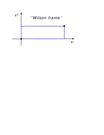
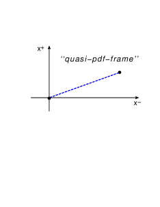
Figure 12: In the left panel the Wilson frame is depicted, while in the right panel the quasi-pdf frame.

The correlation functions with operators defined in eqs. (86)-(88) in the BFKL limit, $j\to 1$, are divergent. A way to regulate such divergence is to consider the “Wilson frame” Balitsky:2013npa which are light-ray operators with point-splitting to regulate UV divergences (see Fig. 12 a))

$${\cal F}^{j}_{p_{1}}(x_{1\perp},x_{2\perp}) \equiv \int_{0}^{\infty}\!du\,u^{1-j}{\cal F}_{p_{1}}(u;x_{1\perp},x_{2\perp})\,,$$ (91)

$${\cal F}_{p_{1}}(u;x_{1\perp},x_{2\perp}) \equiv \int\!dv\,2{\rm Tr}\Big{\{}F_{p_{1}\mu}(up_{1}+vp_{1}+x_{1\perp})[up_{1}+vp_{1},vp_{1}]_{x_{1}}$$ (92)

$$\times[vp_{1}+x_{1\perp},vp_{1}+x_{2\perp}]{F_{p_{1}}}^{\mu}(vp_{1}+x_{2\perp})[vp_{1},up_{1}+vp_{1}]_{x_{2}}\Big{\}}\,.$$

In Ref. Balitsky:2013npa the correlation function of two “Wilson-frames”

$$\langle{\cal F}^{j}_{p_{1}}(x_{1\perp},x_{2\perp}){\cal F}^{j^{\prime}}_{p_{2}}(y_{1\perp},y_{2\perp})\rangle\,,$$ (93)

was calculated in the BFKL limit and the explicit expression for the structure function $C(\Delta,j)$ was derived.

The correlation function of “Wilson-frames” reminds us the correlation function of four $Z^{2}$ currents with $Z={1\over\sqrt{2}}(\phi_{1}+i\phi_{2})$ a renorm-invariant chiral primary operator, in the BFKL limit Balitsky:2009yp in $\cal N$=4 SYM theory, or the correlation function of four electromagnetic currents in QCD which describes the $\gamma^{*}\gamma^{*}$ scattering in the Regge limit Chirilli:2014dcb .

We will show that an alternative gauge-link geometry to regulate the UV divergences present in the BFKL limit is the “quasi-pdf frame” (see Fig. 12 b)). Indeed, we will show that in the limit $\omega=j-1\to 0$, $g\to 0$, and $g^{2}\ll\omega\ll 1$ we get the same result as one obtained in Ref Balitsky:2013npa with “Wilson-frames”.

B.4 Gluon correlation function with “quasi-pdf frame”

As announced in the previous section, we will calculate gluon correlation function with “quasi-pdf frame” in the BFKL limit.

The procedure is the same as the one adopted in Ref. Balitsky:2009yp ; Balitsky:2018irv , i.e., we will apply the high-energy OPE.

The gluon correlation function under consideration is

$$\langle{\cal F}^{j}_{p_{1}}(x_{\perp},y_{\perp}){\cal F}^{j^{\prime}}_{p_{2}}(x^{\prime}_{\perp},y^{\prime}_{\perp})\rangle\,,$$ (94)

with

$${\cal F}^{j}_{p_{1}}(x_{\perp},y_{\perp})=\int_{0}^{+\infty}\!du^{1-j}{\cal F}_{p_{1}}(u;x_{\perp},y_{\perp})\,,$$ (95)

and where now ${\cal F}_{p_{1}}(x,y)$ is taken with quasi-pdf frame (see Fig. 12)

$${\cal F}_{p_{1}}(u;x_{\perp},y_{\perp})=\!\! \int dv{F^{a}}_{p_{1}i}(up_{1}+vp_{1}+x_{\perp})$$ (96)

$$\times[up_{1}+vp_{1}+x_{\perp},vp_{1}+y_{\perp}]^{ab}{{F^{b}}_{p_{1}}}^{i}(vp_{1}+y_{\perp})\,.$$

In coordinate space the Regge limit is achieved considering the limit $x\!\cdot\!p_{2},~{}x^{\prime}\!\cdot\!p_{1}\to\infty$, $y\!\cdot\!p_{1},~{}y^{\prime}\!\cdot\!p_{2}\to-\infty$ and keeping all other components fixed. In this limit, the correlation function (94) factorizes as Balitsky:2009yp

$$\langle{\cal F}_{p_{1}}(x_{\perp},y_{\perp})\rangle\langle{\cal F}_{p_{2}}(x^{\prime}_{\perp},y^{\prime}_{\perp})\rangle\,.$$ (97)

To each factor of (97) we apply the high-energy OPE similarly to what we did in section 5, indeed, using result (18) we have

$$\int_{0}^{+\infty}\!dx^{+}\int_{-\infty}^{0}\!dy^{+}\delta(x^{+}-y^{+}-L)\int_{0}^{+\infty}\!dx^{\prime-}\int_{-\infty}^{0}\!dy^{\prime-}\delta(x^{\prime-}-y^{\prime-}-L^{\prime})$$

$$\times\langle F^{a\,i-}(x^{+},x_{\perp})[nx^{+}+x_{\perp},ny^{+}+y_{\perp}]^{ab}F_{i}^{b\,-}(y^{+},y_{\perp})\rangle_{{\rm Fig.}\ref{Fig:quasipdf-gq-LO}}$$

$$\times\langle F^{a^{\prime}\,k+}(x^{\prime-},x^{\prime}_{\perp})[nx^{\prime-}+x^{\prime}_{\perp},ny^{\prime-}+y^{\prime}_{\perp}]^{a^{\prime}b^{\prime}}F_{k}^{b^{\prime}\,+}(y^{\prime-},y^{\prime}_{\perp})\rangle_{{\rm Fig.}\ref{Fig:quasipdf-gq-LO}}$$

$$={-6N^{2}_{c}\over(x^{+}|y^{+}|)^{3}}\int{d^{2}z_{2}\over\pi^{3}}\,{\cal U}(z_{1},z_{2})\Bigg{[}{-2(x-z_{2},y-z_{2})^{2}_{\perp}+(x-z_{2})^{2}_{\perp}(y-z_{2})^{2}_{\perp}\over\left({(y-z_{2})^{2}_{\perp}\over|y^{+}|}+{(x-z_{2})^{2}_{\perp}\over x^{+}}\right)^{4}}\Bigg{]}$$

$$\times{-6N^{2}_{c}\over(x^{\prime+}|y^{\prime+}|)^{3}}\int{d^{2}z^{\prime}_{2}\over\pi^{3}}\,{\cal U}(z^{\prime}_{1},z^{\prime}_{2})\Bigg{[}{-2(x^{\prime}-z^{\prime}_{2},y^{\prime}-z^{\prime}_{2})^{2}_{\perp}+(x^{\prime}-z^{\prime}_{2})^{2}_{\perp}(y^{\prime}-z^{\prime}_{2})^{2}_{\perp}\over\left({(y^{\prime}-z^{\prime}_{2})^{2}_{\perp}\over|y^{\prime+}|}+{(x^{\prime}-z^{\prime}_{2})^{2}_{\perp}\over x^{\prime+}}\right)^{4}}\Bigg{]}\,.$$ (98)

An important difference between the calculation of a correlation function like (94), and the calculation carried out in section 5, is that here we will not need a model to evaluate the initial condition for the evolution equation of the matrix elements because the initial conditions are fully perturbative and are obtained by calculating in pQCD the dipole-dipole scattering. In section 5, instead, we used a model to evaluate the dipole in the target state.

To proceed, we need the projection of the dipole-Wilson-line operator ${\cal U}(z_{1},z_{2})$ onto the leading-order eigenfunctions, so using the completeness relation, we have

$${\cal U}(z_{1},z_{2})=\int\!d^{2}z_{0}\int{d\nu\over\pi^{2}}\,\nu^{2}\left({z^{2}_{12}\over z^{2}_{10}z^{2}_{20}}\right)^{\gamma}{\cal U}(\nu,z_{0})\,,$$ (99)

with $\gamma={1\over 2}+i\nu$ and ${\bar{\gamma}}=1-\gamma$, and where we defined

$${\cal U}(\nu,z_{0})\equiv\int{d^{2}z^{\prime}_{1}d^{2}z^{\prime}_{2}\over\pi^{2}z^{\prime 4}_{12}}\left({z^{\prime 2}_{12}\over z^{\prime 2}_{10}z^{\prime 2}_{20}}\right)^{\bar{\gamma}}{\cal U}(z^{\prime}_{1},z^{\prime}_{2})\,.$$ (100)

We also need the solution of the evolution equation for the dipole-Wilson-line operator in the linear case, i.e. the BFKL equation,

$${\cal U}^{Y_{a}}(\nu,z_{0})=e^{(Y_{a}-Y_{0})\aleph(\nu)}{\cal U}^{Y_{0}}(\nu,z_{0})\,,$$ (101)

$${\cal U}^{Y_{b}}(\nu,z^{\prime}_{0})=e^{(Y_{0}+Y_{b})\aleph(\nu)}{\cal U}^{Y_{0}}(\nu,z^{\prime}_{0})\,.$$ (102)

where $\aleph(\nu)=\aleph(\gamma(\nu))$ with $\gamma={1\over 2}+i\nu$. The resummation parameter in coordinate space is Balitsky:2009yp

$$Y_{a}={1\over 2}\ln{2L^{2}\over(x-y)^{2}_{\perp}}\,,~{}~{}~{}~{}~{}~{}~{}~{}Y_{b}={1\over 2}\ln{2L^{\prime 2}\over(x^{\prime}-y^{\prime})^{2}_{\perp}}\,.$$ (103)

Indeed, in coordinate space, we already observed above, $L,L^{\prime}\to\infty$ while the other components are kept fixed. To have an intuitive picture, one has to recall the more familiar case of $\gamma^{*}\gamma^{*}$ process, and think to the $L$, and $L^{\prime}$ as conjugated to the center of mass energy of the virtual photon-target system, and $(x-y)^{2}_{\perp}$, and $(x^{\prime}-y^{\prime})^{2}_{\perp}$ conjugated to the virtuality of the photon.

So, using (99), the dipole-dipole amplitude with BFKL resummation is (see section C for details of the calculation)

$$\langle{\cal U}^{Y_{a}}(z_{1},z_{2}){\cal U}^{Y_{b}}(z^{\prime}_{1},z^{\prime}_{2})\rangle$$

$$=-{\alpha^{2}_{s}(N^{2}_{c}-1)\over N^{2}_{c}}\int{d\nu\over\pi}{16\,\nu^{2}\over(1+4\nu^{2})^{2}}\Big{(}{2LL^{\prime}\over|(x-y)_{\perp}||(x^{\prime}-y^{\prime})_{\perp}|}\Big{)}^{\aleph(\gamma)}$$

$$~{}~{}~{}\times{\Gamma^{2}({1\over 2}+i\nu)\Gamma(-2i\nu)\over\Gamma^{2}({1\over 2}-i\nu)\Gamma(1+2i\nu)}\left({z^{2}_{12}z^{\prime 2}_{12}\over(X-X^{\prime})^{4}}\right)^{\gamma}\,.$$ (104)

Using eq. (104), and the result of projection eq. (21), from eq. (98) we get

$$\int_{0}^{+\infty}\!dx^{+}\int_{-\infty}^{0}\!dy^{+}\delta(x^{+}-y^{+}-L)\int_{0}^{+\infty}\!dx^{\prime-}\int_{-\infty}^{0}\!dy^{\prime-}\delta(x^{\prime-}-y^{\prime-}-L^{\prime})$$

$$~{}~{}\times\!\langle F^{a\,i-}(x^{+},x_{\perp})[nx^{+}+x_{\perp},ny^{+}+y_{\perp}]^{ab}F_{i}^{b\,-}(y^{+},y_{\perp})\rangle_{{\rm Fig.}\ref{Fig:quasipdf-gq-LO}}$$

$$~{}~{}\times\!\langle F^{a^{\prime}\,k+}(x^{\prime-},x^{\prime}_{\perp})[nx^{\prime-}+x^{\prime}_{\perp},ny^{\prime-}+y^{\prime}_{\perp}]^{a^{\prime}b^{\prime}}F_{k}^{b^{\prime}\,+}(y^{\prime-},y^{\prime}_{\perp})\rangle_{{\rm Fig.}\ref{Fig:quasipdf-gq-LO}}$$

$$={-9\alpha^{2}_{s}N^{4}_{c}\over LL^{\prime}\Delta^{2}_{\perp}\Delta^{\prime 2}_{\perp}}\int{d\nu\over\pi^{5}}{64\,\nu^{2}\over(1+4\nu^{2})^{2}}{\gamma^{10}\Gamma(1-2\gamma)\Gamma^{8}(\gamma)\over\Gamma(2\gamma)\Gamma^{2}(2\gamma+2)}{\left(\Delta^{2}_{\perp}\Delta^{\prime 2}_{\perp}\over(X-X^{\prime})_{\perp}^{4}\right)^{\gamma}}\!\!\left({2LL^{\prime}\over|\Delta^{2}_{\perp}||\Delta^{\prime 2}_{\perp}|}\right)^{\!\aleph(\gamma)}\,,$$ (105)

where we defined $X_{\perp}={x_{\perp}+y_{\perp}\over 2}$ and the same for $X^{\prime}_{\perp}$, and where we used $N^{2}_{c}-1\to N^{2}_{c}$ in the large $N_{c}$ limit. From (105) we can calculate the correlation function of the $j$-dependent operators

$$\langle{\cal F}_{p_{1}}^{j}(x_{\perp},y_{\perp}){\cal F}_{p_{2}}^{j^{\prime}}(x^{\prime}_{\perp},y^{\prime}_{\perp})\rangle$$

$$=-{9\alpha^{2}_{s}N^{4}_{c}\over LL^{\prime}\Delta^{2}_{\perp}\Delta^{\prime 2}_{\perp}}\left(s\over 2\right)^{j-1}\int_{0}^{+\infty}\!dLL^{1-j}\int_{0}^{+\infty}\!dL^{\prime}L^{\prime 1-j^{\prime}}\theta(2LL^{\prime}-(X-X^{\prime})^{2}_{\perp})$$

$$~{}\times\!\!\int{d\nu\over\pi^{5}}{64\,\nu^{2}\over(1+4\nu^{2})^{2}}{\gamma^{10}\Gamma(1-2\gamma)\Gamma^{8}(\gamma)\over\Gamma(2\gamma)\Gamma^{2}(2\gamma+2)}{\left(\Delta^{2}_{\perp}\Delta^{\prime 2}_{\perp}\over(X-X^{\prime})_{\perp}^{4}\right)^{\gamma}}\!\!\left({2LL^{\prime}\over|\Delta^{2}_{\perp}||\Delta^{\prime 2}_{\perp}|}\right)^{\!\aleph(\gamma)}\,,$$ (106)

where we used

$${\cal F}_{p_{1}}^{j}(x_{\perp},y_{\perp})=\!\! \left(s\over 2\right)^{j-1\over 2}\int_{0}^{+\infty}dL\,L^{1-j}\int dx^{+}{F^{a-}}_{\xi}(x^{+}+L,x_{\perp})$$ (107)

$$\times[(x^{+}+L)n+x_{\perp},nx^{+}+y_{\perp}]^{ab}F^{b\,-\xi}(x^{+},y_{\perp})\,,$$

and similarly for ${\cal F}_{p_{2}}^{j}(x^{\prime}_{\perp},y^{\prime}_{\perp})$. The $\theta(2LL^{\prime}-(X-X^{\prime})^{2}_{\perp})$-function ensures that the longitudinal size of two quasi-pdf frames are greater than the relative transverse separation. Performing the integration over $L$ and $L^{\prime}$ we arrive at

$$\langle{\cal F}^{j}_{p_{1}}(x_{\perp},y_{\perp}){\cal F}^{j^{\prime}}_{p_{2}}(x^{\prime}_{\perp},y^{\prime}_{\perp})\rangle$$

$$=18{\alpha^{2}_{s}N^{4}_{c}\over\pi^{4}}\left(s\over 2\right)^{j-1}\int d\nu\,{2^{\omega}\,(\Delta^{2}_{\perp}\Delta^{\prime 2}_{\perp})^{\gamma-1-{\aleph(\gamma)\over 2}}\over[(X-X^{\prime})^{2}_{\perp}]^{2\gamma+j-1-\aleph(\gamma)}}\,{\theta({\rm Re}[\omega-\aleph(\gamma)])\over\omega-\aleph(\gamma)}$$

$$~{}~{}\times{(1-2\gamma)^{2}\over(1-\gamma)^{2}}{\Gamma(1-2\gamma)\Gamma^{8}(1+\gamma)\over\Gamma(2\gamma)\Gamma^{2}(2\gamma+2)}\delta(\omega-\omega^{\prime})\,.$$ (108)

To perform last integration we change variable $\nu\to\gamma={1\over 2}+i\nu$ and consider the “DGLAP” limit $\alpha_{s}\ll\omega=j-1\ll 0$

$$\langle{\cal F}_{p_{1}}^{j}(x_{\perp},y_{\perp}){\cal F}_{p_{2}}^{j^{\prime}}(x^{\prime}_{\perp},y^{\prime}_{\perp})\rangle$$

$$=-i\,18{\alpha^{2}_{s}N^{4}_{c}\over\pi^{4}}\int_{{1\over 2}-i\infty}^{{1\over 2}+i\infty}\!\!d\gamma\,{s^{\omega}\,(\Delta^{2}_{\perp}\Delta^{\prime 2}_{\perp})^{\gamma-1-{\aleph(\gamma)\over 2}}\over[(X-X^{\prime})^{2}_{\perp}]^{2\gamma+j-1-\aleph(\gamma)}}\,{\theta({\rm Re}[\omega-\aleph(\gamma)])\over\omega-\aleph(\gamma)}$$

$$~{}~{}\times{(1-2\gamma)^{2}\over(1-\gamma)^{2}}{\Gamma(1-2\gamma)\Gamma^{8}(1+\gamma)\over\Gamma(2\gamma)\Gamma^{2}(2\gamma+2)}\delta(\omega-\omega^{\prime})\,.$$ (109)

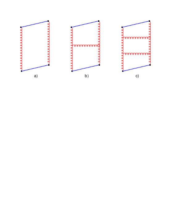
Figure 13: First three order diagrams for the correlator of two “quasi-PDF” frames. Diagrams a) and b) are not included in the product of two dipole Wilson-line operators.

In eq. (109), we can close the contour to the right of all the residues and consider only the left most one which will give the leading contribution. However, we observe that there are two residues to consider. The first, $\gamma=1-{\alpha_{s}\over\omega}$, reproduces the general expected result of eq. (79) in the high-energy limit. The second one, $\gamma=1$, cancels out the diagrams a) and b) in Fig. 13 which are not included into the high-energy OPE formalism. To see this, one has to consider diagram in Fig. 2 and expand the Wilson line operator to two gluon approximation. In this way, one observes that from this expansion, the first diagram that obtains is the one in figure 13c (plus permutations). Thus, diagrams in Fig. 13a) and b) are absent from the high-energy OPE, but they have to be included in the calculation of this correlation function. The contribution of diagram in figure 13 a) (diagram b) is higher order) will exactly cancel the contribution from the residue at the point $\gamma=1$. Diagram in Fig. 13 a) has been calculated in Ref. Balitsky:2018irv , so we do not need to calculate it again, rather, we will show that it get canceled from the residue at $\gamma=1$ also in the case of quasi-pdf frame. We remind the reader that in Ref. Balitsky:2018irv (see also Ref. Balitsky:2013npa ) the gluon correlation function was considered with Wilson frames (see Fig. 12).

Taking the residue at $\aleph(\gamma^{*})-\omega=0$ we have

$$\langle{\cal F}_{p_{1}}^{j}(x_{\perp},y_{\perp}){\cal F}_{p_{2}}^{j^{\prime}}(x^{\prime}_{\perp},y^{\prime}_{\perp})\rangle$$

$$=36{\alpha^{2}_{s}N^{4}_{c}\over\pi^{3}}{s^{\omega}\,(\Delta^{2}_{\perp}\Delta^{\prime 2}_{\perp})^{\gamma^{*}-1-{\omega\over 2}}\over[(X-X^{\prime})^{2}_{\perp}]^{2\gamma^{*}}}\,{(1-2\gamma^{*})^{2}\over(1-\gamma^{*})^{2}}{\Gamma(1-2\gamma^{*})\Gamma^{8}(1+\gamma^{*})\over\Gamma(2\gamma^{*})\Gamma^{2}(2\gamma^{*}+2)}{\delta(\omega-\omega^{\prime})\over\aleph^{\prime}(\gamma^{*})}\,.$$ (110)

Here $|\Delta_{\perp}||\Delta^{\prime}_{\perp}|$ is the IR cut-off and $\aleph^{\prime}(\gamma)={d\over d\gamma}\aleph(\gamma)$. Comparing (110) with (79), we have two equations $2\gamma^{*}-2-\omega=\gamma_{a}$ and $2\gamma^{*}=\Delta-1$, from which we get $\gamma_{a}+\omega=\Delta-3$ in agreement with result obtained in Ref. Balitsky:2018irv .

In the limit $\alpha_{s}\ll\omega\ll 1$ we have $\gamma^{*}=1-{\bar{\alpha}_{s}\over\omega}$ with $\bar{\alpha}_{s}={\alpha_{s}N_{c}\over\pi}$, and result (110) becomes

$$\langle{\cal F}_{p_{1}}^{j}(x_{\perp},y_{\perp}){\cal F}_{p_{2}}^{j^{\prime}}(x^{\prime}_{\perp},y^{\prime}_{\perp})\rangle\simeq-N^{2}_{c}{(|\Delta_{\perp}\Delta^{\prime}_{\perp}|)^{-{2\bar{\alpha}_{s}\over\omega}-\omega}\over[(X-X^{\prime})^{2}_{\perp}]^{2-2{\bar{\alpha}_{s}\over\omega}}}{\omega\over 2\pi}s^{\omega}\delta(j-j^{\prime})\,.$$ (111)

Result (111) coincides with the one obtained in Refs. Balitsky:2013npa ; Balitsky:2018irv and is consistent with the general result for two-point correlation function eq. (79).

What we are left to do is the calculation of the residue at $\gamma=1$ and show that it coincides with the one calculated in Balitsky:2018irv , thus canceling the contribution of diagrams a) and b) in figure 13. So, we start from eq. (109) which we can rewrite as

$$\langle{\cal F}_{p_{1}}^{j}(x_{\perp},y_{\perp}){\cal F}_{p_{2}}^{j^{\prime}}(x^{\prime}_{\perp},y^{\prime}_{\perp})\rangle$$

$$=-i\,18{\alpha^{2}_{s}N^{4}_{c}\over\pi^{4}}\int_{{1\over 2}-i\infty}^{{1\over 2}+i\infty}\!\!d\gamma\,{s^{\omega}\,(\Delta^{2}_{\perp}\Delta^{\prime 2}_{\perp})^{\gamma-1-{\aleph(\gamma)\over 2}}\over[(X-X^{\prime})^{2}_{\perp}]^{2\gamma+j-1-\aleph(\gamma)}}\,{\theta({\rm Re}[\omega-\aleph(\gamma)])\over\omega-\aleph(\gamma)}$$

$$~{}~{}\times{(1-2\gamma)^{2}\over 2(1-\gamma)^{3}}{\Gamma(3-2\gamma)\Gamma^{8}(1+\gamma)\over\Gamma(2\gamma)\Gamma^{2}(2\gamma+2)}\delta(j-j^{\prime})\,.$$ (112)

The residue at $\gamma=1$ is

$$\langle{\cal F}_{p_{1}}^{j}(x_{\perp},y_{\perp}){\cal F}_{p_{2}}^{j^{\prime}}(x^{\prime}_{\perp},y^{\prime}_{\perp})\rangle=\!\! -{N^{2}_{c}s^{\omega}\omega\over\pi[(X-X^{\prime})^{2}_{\perp}]^{\omega+2}}\left({\bar{\alpha}_{s}\over 3\omega}-{1\over 2}-{\bar{\alpha}_{s}\over\omega}\ln{(X-X^{\prime})^{2}_{\perp}\over|\Delta_{\perp}||\Delta^{\prime}_{\perp}|}\right)\delta(j-j^{\prime})$$

$$\simeq\!\! {N^{2}_{c}s^{\omega}\omega\over 2\pi[(X-X^{\prime})^{2}_{\perp}]^{\omega+2}}\left(1+2{\bar{\alpha}_{s}\over\omega}\ln{(X-X^{\prime})^{2}_{\perp}\over|\Delta_{\perp}||\Delta^{\prime}_{\perp}|}\right)\delta(j-j^{\prime})\,,$$ (113)

where we used $\bar{\alpha}_{s}\ll\omega\ll 1$ and $\bar{\alpha}_{s}\ll\bar{\alpha}_{s}\ln{(X-X^{\prime})^{2}_{\perp}\over|\Delta_{\perp}||\Delta^{\prime}_{\perp}|}$. Result (113) coincides exactly with eq. (5.40) of reference Balitsky:2018irv .

In conclusion, in this section we have proven that the Wilson-frame regulator and the quasi-pdf frame regulator give the same result in the calculation of the two-point correlation function in the high-energy, $j\to 1$, limit. This justifies the use of the HE-OPE for the calculation of the high-energy behavior of the LT and NLT gluon distributions.

Appendix C Dipole-dipole scattering

In this section we calculate the dipole-dipole scattering. Using (99), we have

$$\langle{\cal U}^{Y_{a}}(z_{1},z_{2}){\cal U}^{Y_{b}}(z^{\prime}_{1},z^{\prime}_{2})\rangle$$

$$=\int{d\nu\over\pi^{2}}\,\nu^{2}\!\int d^{2}z_{0}\left({z^{2}_{12}\over z_{10}^{2}z_{20}^{2}}\right)^{\gamma}\!\!\int\!\!{d\nu^{\prime}\over\pi^{2}}\,\nu^{\prime 2}\!\int\!\!d^{2}z^{\prime}_{0}\left({z^{\prime 2}_{12}\over z^{\prime 2}_{10}z^{\prime 2}_{20}}\right)^{\gamma^{\prime}}\!\!\langle{\cal U}^{Y_{a}}(z_{0},\nu){\cal U}^{Y_{b}}(z^{\prime}_{0},\nu^{\prime})\rangle\,,$$ (114)

where, as we explained above, the evolution parameters are $Y_{a}={1\over 2}\ln{2L^{2}\over(x-y)^{2}_{\perp}}$ and $Y_{b}={1\over 2}\ln{2L^{\prime 2}\over(x^{\prime}-y^{\prime})^{2}_{\perp}}$. Assuming that $Y_{0}$ is the initial condition for the evolution, the dipole-dipole scattering with BFKL resummation is

$$\langle{\cal U}^{Y_{a}}(z_{0},\nu){\cal U}^{Y_{b}}(z_{0},\nu)\rangle=\!\!\! \Big{\langle}e^{(Y_{a}-Y_{0})\aleph(\nu)}{\cal U}^{Y_{0}}(\nu,z_{0})e^{(Y_{0}+Y_{b})\aleph(\nu)}{\cal U}^{Y_{0}}(\nu,z_{0})\Big{\rangle}$$ (115)

$$\times e^{(Y_{a}+Y_{b})\aleph(\nu)}{-\alpha_{s}^{2}(N_{c}^{2}-1)\over 4N_{c}^{2}}{16\pi^{2}\over\nu^{2}(1+4\nu^{2})^{2}}$$

$$\times\Big{[}\delta(z_{0}-z^{\prime}_{0})\delta(\nu+\nu^{\prime})+{2^{1-4i\nu}\delta(\nu-\nu^{\prime})\over\pi|z_{0}-z^{\prime}_{0}|^{2-4i\nu}}{\Gamma\big{(}{1\over 2}+i\nu\big{)}\Gamma(1-i\nu)\over\Gamma(i\nu)\Gamma\big{(}{1\over 2}-i\nu\big{)}}\Big{]}\,.$$

Substituting (115) in eq. (114) we have

$$\langle{\cal U}^{Y_{a}}(z_{0},\nu){\cal U}^{Y_{b}}(z_{0},\nu)\rangle=\!\!\! -{\alpha^{2}_{s}(N^{2}_{c}-1)\over N^{2}_{c}}\int{d\nu\over\pi}{16\,\nu^{2}\over(1+4\nu^{2})^{2}}\Big{(}{2LL^{\prime}\over|(x-y)_{\perp}||(x^{\prime}-y^{\prime})_{\perp}|}\Big{)}^{\aleph(\gamma)}$$ (116)

$$\times{\Gamma^{2}({1\over 2}+i\nu)\Gamma(-2i\nu)\over\Gamma^{2}({1\over 2}-i\nu)\Gamma(1+2i\nu)}\left({z^{2}_{12}z^{\prime 2}_{12}\over(X-X^{\prime})^{4}}\right)^{\gamma}\,,$$

with $X={x_{\perp}+y_{\perp}\over 2}$ and the same for $X^{\prime}$, and where we used

$$\int d^{2}z_{0}\left({z^{2}_{12}\over z_{10}^{2}z_{20}^{2}}\right)^{\gamma}\left({z^{\prime 2}_{12}\over(z^{\prime}_{1}-z_{0})^{2}(z^{\prime}_{2}-z_{0})^{2}}\right)^{1-\gamma}$$

$$=\left\{\left({z^{2}_{12}z^{\prime 2}_{12}\over(X-X^{\prime})^{4}}\right)^{\gamma}\pi{\Gamma^{2}({1\over 2}+i\nu)\Gamma(-2i\nu)\over\Gamma^{2}({1\over 2}-i\nu)\Gamma(1+2i\nu)}+\nu\leftrightarrow-\nu\right\}\,,$$ (117)

and

$$\int{d\nu d\nu^{\prime}\over\pi^{4}}\nu^{2}\nu^{\prime 2}\int d^{2}z_{0}\left({z^{2}_{12}\over z_{10}^{2}z_{20}^{2}}\right)^{\gamma}\int d^{2}z^{\prime}_{0}\left({z^{\prime 2}_{12}\over z^{\prime 2}_{10}z^{\prime 2}_{20}}\right)^{\gamma^{\prime}}$$

$$\times{2^{1-4i\nu}\delta(\nu-\nu^{\prime})\over\pi|z_{0}-z^{\prime}_{0}|^{2-4i\nu}}{\Gamma({1\over 2}+i\nu)\Gamma(1-i\nu)\over\Gamma(i\nu)\Gamma({1\over 2}-i\nu)}$$

$$=\int{d\nu\over\pi^{4}}\nu^{4}\left\{\left({z^{2}_{12}z^{\prime 2}_{12}\over(X-X^{\prime})^{4}}\right)^{\gamma}\pi{\Gamma^{2}({1\over 2}+i\nu)\Gamma(-2i\nu)\over\Gamma^{2}({1\over 2}-i\nu)\Gamma(1+2i\nu)}+\nu\leftrightarrow-\nu\right\}\,.$$ (118)

Appendix D LT and NLT pseudo-PDF: analytic expression

In this section we evaluate the inverse Mellin transform of eq. (49) which is the approximated result of eq. (48). To perform the inverse Mellin, regardless of whether $\ln{4\over Q_{s}^{2}|z|^{2}}$ is positive or negative, is

$$G_{\rm p}(x_{B},z^{2})=\!\!\! {N^{2}_{c}\,Q^{2}_{s}\sigma_{0}\over 16\bar{\alpha}_{s}\pi^{3}}{1\over 2\pi i}\int_{1-i\infty}^{1+i\infty}{d\omega\over\omega}\,\left({2\over x_{B}^{2}|z|^{2}M_{N}^{2}}\right)^{\omega\over 2}\left({4\over Q^{2}_{s}|z|^{2}}\right)^{{\bar{\alpha}_{s}\over\omega}}$$

$$\times\left(1+{Q_{s}^{2}|z|^{2}\over 5}\right)+O\!\left({Q_{s}^{4}|z|^{4}\over 16}\right)$$

$$=\!\!\! {N^{2}_{c}Q_{s}^{2}\sigma_{0}\over 16\pi^{3}\bar{\alpha}_{s}}\left(1+{Q_{s}^{2}|z|^{2}\over 5}\right)I_{0}(h)+O\!\left({Q_{s}^{4}|z|^{4}\over 16}\right)\,,$$ (119)

with $h$ defined as

$$h=\left[2\bar{\alpha}_{s}\left|\ln{4\over|z|^{2}Q_{s}^{2}}\right|\ln{2\over x_{B}^{2}|z^{2}|M^{2}_{N}}\right]^{1\over 2}\,.$$ (120)

In Fig. 14 we show that eq. (48) can be well approximated by result (119).

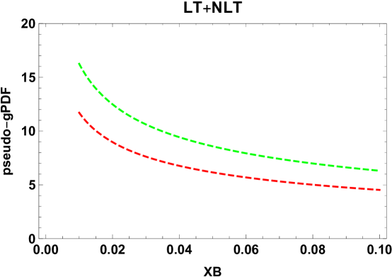
Figure 14: Comparing the numerical evaluation of eq. (48) (red dashed curve) with its approximated analytic result, eq. (119) (green dashed curve).

Appendix E LT and NLT quasi-PDF: analytic expression

To perform the inverse Mellin transform in eq. (56), we have to distinguish two cases. The first case is when $\ln{4P_{\xi}^{2}x_{B}^{2}\over Q^{2}_{s}}<0$, and the inverse Mellin transform is

$$G_{\rm q}(x_{B},P_{\xi}) \simeq{N^{2}_{c}\,Q^{2}_{s}\,\sigma_{0}\over 16\bar{\alpha}_{s}\pi^{3}}\left[{\ln\left(-{Q_{s}^{2}\over 4P_{\xi}^{2}x_{B}^{2}}-i\epsilon\right)\over\ln\left(-{2P_{\xi}^{2}\over M^{2}_{N}}+i\epsilon\right)}\left(J_{0}(m)-J_{2}(m)-{2\over m}J_{1}(m)\right)\right.$$ (121)

$$\left.~{}~{}~{}~{}~{}~{}~{}~{}~{}~{}~{}~{}~{}~{}~{}~{}~{}+{2Q_{s}^{2}\over 5P_{\xi}^{2}x_{B}^{2}}\left({2\bar{\alpha}_{s}\ln\left(-{Q_{s}^{2}\over 4P_{\xi}^{2}x_{B}^{2}}-i\epsilon\right)\over\ln\left(-{2P_{\xi}^{2}\over M_{N}^{2}}+i\epsilon\right)}\right)^{1\over 2}J_{1}(m)\right]\,,$$

where we defined

$$m\equiv\left[2\bar{\alpha}_{s}\ln\left(-{Q_{s}^{2}\over 4P_{\xi}^{2}x_{B}^{2}}-i\epsilon\right)\ln\left(-{2P_{\xi}^{2}\over M_{N}^{2}}+i\epsilon\right)\right]^{1\over 2}\,.$$ (122)

Figure 15: We compare the real part of eq. (55) (magenta-dashed curve) with its approximation, real part of eq. (121) (blue curve). This is the case $\ln{4P_{\xi}^{2}x_{B}^{2}\over Q^{2}_{s}}<0$, with $P_{\xi}=4$  GeV, and $x_{B}\in[0.001,0.04]$.

The second case is when $\ln{4P_{\xi}^{2}x_{B}^{2}\over Q^{2}_{s}}>0$, and the inverse Mellin transform is

$$G_{q}(x_{B},P_{\xi}) \!\!\simeq-{N^{2}_{c}Q_{s}^{2}\sigma_{0}\over 16\bar{\alpha}_{s}\pi^{3}}\left[{\ln\left(-{4P_{\xi}^{2}x_{B}^{2}\over Q_{s}^{2}}+i\epsilon\right)\over\ln\left(-{2P_{\xi}^{2}\over M^{2}_{N}}+i\epsilon\right)}\left(I_{0}(\tilde{m})+I_{2}(\tilde{m})-{2\over\tilde{m}}I_{1}(\tilde{m})\right)\right.$$ (123)

$$\left.~{}~{}~{}+{2Q_{s}^{2}\over 5P^{2}_{\xi}x_{B}^{2}}\left({2\bar{\alpha}_{s}}\ln\left(-{4P_{\xi}^{2}x_{B}^{2}\over Q_{s}^{2}}+i\epsilon\right)\over\ln\left(-{2P_{\xi}^{2}\over M^{2}_{N}}+i\epsilon\right)\right)^{1\over 2}I_{1}(\tilde{m})\right]\,,$$

and where we defined

$$\tilde{m}\equiv\left[2\bar{\alpha}_{s}\ln\left(-{4P_{\xi}^{2}x_{B}^{2}\over Q_{s}^{2}}+i\epsilon\right)\ln\left(-{2P_{\xi}^{2}\over M_{N}^{2}}+i\epsilon\right)\right]^{1\over 2}\,.$$ (124)

References

• (1) K. Cichy and M. Constantinou, A guide to light-cone PDFs from Lattice QCD: an overview of approaches, techniques and results, Adv. High Energy Phys. 2019 (2019) 3036904 [1811.07248].
• (2) X. Ji, Y.-S. Liu, Y. Liu, J.-H. Zhang and Y. Zhao, Large-momentum effective theory, Rev. Mod. Phys. 93 (2021) 035005 [2004.03543].
• (3) K. Cichy, Progress in $x$-dependent partonic distributions from lattice QCD, in 38th International Symposium on Lattice Field Theory, 10, 2021 [2110.07440].
• (4) V. Braun and D. Müller, Exclusive processes in position space and the pion distribution amplitude, Eur. Phys. J. C 55 (2008) 349 [0709.1348].
• (5) G.S. Bali et al., Pion distribution amplitude from Euclidean correlation functions, Eur. Phys. J. C 78 (2018) 217 [1709.04325].
• (6) G.S. Bali, V.M. Braun, B. Gläßle, M. Göckeler, M. Gruber, F. Hutzler et al., Pion distribution amplitude from Euclidean correlation functions: Exploring universality and higher-twist effects, Phys. Rev. D 98 (2018) 094507 [1807.06671].
• (7) L. Del Debbio, T. Giani, J. Karpie, K. Orginos, A. Radyushkin and S. Zafeiropoulos, Neural-network analysis of Parton Distribution Functions from Ioffe-time pseudodistributions, JHEP 02 (2021) 138 [2010.03996].
• (8) Y.-Q. Ma and J.-W. Qiu, Extracting Parton Distribution Functions from Lattice QCD Calculations, Phys. Rev. D 98 (2018) 074021 [1404.6860].
• (9) Y.-Q. Ma and J.-W. Qiu, Exploring Partonic Structure of Hadrons Using ab initio Lattice QCD Calculations, Phys. Rev. Lett. 120 (2018) 022003 [1709.03018].
• (10) X. Ji, Parton Physics on a Euclidean Lattice, Phys. Rev. Lett. 110 (2013) 262002 [1305.1539].
• (11) A.V. Radyushkin, Quasi-parton distribution functions, momentum distributions, and pseudo-parton distribution functions, Phys. Rev. D 96 (2017) 034025 [1705.01488].
• (12) K. Orginos, A. Radyushkin, J. Karpie and S. Zafeiropoulos, Lattice QCD exploration of parton pseudo-distribution functions, Phys. Rev. D 96 (2017) 094503 [1706.05373].
• (13) B. Joó, J. Karpie, K. Orginos, A.V. Radyushkin, D.G. Richards and S. Zafeiropoulos, Parton Distribution Functions from Ioffe Time Pseudodistributions from Lattice Calculations: Approaching the Physical Point, Phys. Rev. Lett. 125 (2020) 232003 [2004.01687].
• (14) HadStruc collaboration, Unpolarized gluon distribution in the nucleon from lattice quantum chromodynamics, Phys. Rev. D 104 (2021) 094516 [2107.08960].
• (15) I. Balitsky, High-energy QCD and Wilson lines, hep-ph/0101042.
• (16) I. Balitsky, NLO BFKL and anomalous dimensions of light-ray operators, Int. J. Mod. Phys. Conf. Ser. 25 (2014) 1460024.
• (17) I. Balitsky, V. Kazakov and E. Sobko, Two-point correlator of twist-2 light-ray operators in N=4 SYM in BFKL approximation, 1310.3752.
• (18) I. Balitsky, V. Kazakov and E. Sobko, Structure constant of twist-2 light-ray operators in the Regge limit, Phys. Rev. D 93 (2016) 061701 [1506.02038].
• (19) I. Balitsky, V. Kazakov and E. Sobko, Three-point correlator of twist-2 light-ray operators in N=4 SYM in BFKL approximation, 1511.03625.
• (20) I. Balitsky, Structure constants of twist-two light-ray operators in the triple Regge limit, JHEP 04 (2019) 042 [1812.07044].
• (21) I. Balitsky, W. Morris and A. Radyushkin, Gluon Pseudo-Distributions at Short Distances: Forward Case, Phys. Lett. B 808 (2020) 135621 [1910.13963].
• (22) I. Balitsky, W. Morris and A. Radyushkin, Short-Distance Structure of Unpolarized Gluon Pseudodistributions, 2111.06797.
• (23) I. Balitsky, Operator expansion for high-energy scattering, Nucl. Phys. B463 (1996) 99 [hep-ph/9509348].
• (24) Y.V. Kovchegov, Small-x $F_{2}$ structure function of a nucleus including multiple pomeron exchanges, Phys. Rev. D60 (1999) 034008 [hep-ph/9901281].
• (25) J. Jalilian-Marian, A. Kovner, A. Leonidov and H. Weigert, The Wilson renormalization group for low x physics: Towards the high density regime, Phys. Rev. D59 (1998) 014014 [hep-ph/9706377].
• (26) E. Ferreiro, E. Iancu, A. Leonidov and L. McLerran, Nonlinear gluon evolution in the color glass condensate. II, Nucl. Phys. A703 (2002) 489 [hep-ph/0109115].
• (27) E. Iancu, A. Leonidov and L.D. McLerran, Nonlinear gluon evolution in the color glass condensate. I, Nucl. Phys. A692 (2001) 583 [hep-ph/0011241].
• (28) I. Balitsky and G.A. Chirilli, NLO evolution of color dipoles in N=4 SYM, Nucl.Phys. B822 (2009) 45 [0903.5326].
• (29) I. Balitsky and G.A. Chirilli, High-energy amplitudes in N=4 SYM in the next-to-leading order, Int. J. Mod. Phys. A25 (2010) 401 [0911.5192].
• (30) I. Balitsky and G.A. Chirilli, Photon impact factor in the next-to-leading order, Phys.Rev. D83 (2011) 031502 [1009.4729].
• (31) I. Balitsky and G.A. Chirilli, Photon impact factor and $k_{T}$-factorization for DIS in the next-to-leading order, Phys. Rev. D 87 (2013) 014013 [1207.3844].
• (32) K. Golec-Biernat and M. Wüsthoff, Saturation effects in deep inelastic scattering at low $Q^{2}$ and its implications on diffraction, Phys. Rev. D59 (1998) 014017 [hep-ph/9807513].
• (33) L.D. McLerran and R. Venugopalan, Computing quark and gluon distribution functions for very large nuclei, Phys. Rev. D49 (1994) 2233 [hep-ph/9309289].
• (34) I.I. Balitsky, Quark Contribution to the Small-$x$ Evolution of Color Dipole, Phys. Rev. D 75 (2007) 014001 [hep-ph/0609105].
• (35) Y. Kovchegov and H. Weigert, Triumvirate of Running Couplings in Small-$x$ Evolution, Nucl. Phys. A 784 (2007) 188 [hep-ph/0609090].
• (36) I. Balitsky and G.A. Chirilli, Next-to-leading order evolution of color dipoles, Phys. Rev. D 77 (2008) 014019 [0710.4330].
• (37) T. Jaroszewicz, Gluonic Regge Singularities and Anomalous Dimensions in QCD, Phys. Lett. B 116 (1982) 291.
• (38) V.S. Fadin and L.N. Lipatov, BFKL pomeron in the next-to-leading approximation, Phys. Lett. B429 (1998) 127 [hep-ph/9802290].
• (39) I.I. Balitsky and V.M. Braun, Evolution Equations for QCD String Operators, Nucl. Phys. B 311 (1989) 541.
• (40) V.M. Braun, A. Vladimirov and J.-H. Zhang, Power corrections and renormalons in parton quasidistributions, Phys. Rev. D 99 (2019) 014013 [1810.00048].
• (41) A.V. Belitsky, S.E. Derkachov, G.P. Korchemsky and A.N. Manashov, Superconformal operators in N=4 superYang-Mills theory, Phys. Rev. D 70 (2004) 045021 [hep-th/0311104].
• (42) G.A. Chirilli and Y.V. Kovchegov, $\gamma^{*}\gamma^{*}$ Cross Section at NLO and Properties of the BFKL Evolution at Higher Orders, JHEP 05 (2014) 099 [1403.3384].