Comparative analysis of the Compton ionization of Hydrogen and Positronium.

Abstract

The paper deals with the Compton disintegration of positronium and a comparison of the differential cross sections of this process with the similar cross sections in the case of the Compton ionization of the hydrogen atom. Special attention is paid to the resonances arising, when the electron and positron move parallel to each other in continuum states with the same velocities and zero relative momentum. It is likely that a manifestation of this effect in the double differential cross section is found as an additional peak, which grows with a decrease in the photon energy.

1. INTRODUCTION

Traditionally, we believe that the hydrogen atom is the simplest quantum system, about which everything is known and which is used as a basic target for the study of various atomic reactions: excitation, ionization, capture, photoprocesses, etc. It is really so, but there is one more simple quantum object with the same properties, this is the positronium (the so-called exotic atom). The singlet parapositronium state lives 0.12 ns, the triplet orthopositronium state lives 138.6 ns. These values can be calculated theoretically AB . A hydrogen atom lives on average 0.1 - 10 ns in an excited state, although highly excited states can exist in vacuum for up to several seconds. In this sense the lifetime of different forms of positronium is quite comparable with the lifetime of an excited hydrogen atom, which means that these atoms can be experimentally studied with the same devices. Beyond the lifetime, the main difference between hydrogen and positronium is the mass of the positively charged particles: the proton mass is $M=1836.4$ a.u., whereas the mass of the positron (equal to that of the electron) is $m=1$ a.u., and this difference results in significant differences in the scattering cross sections.

In paper EPJD20 , the Compton ionization of a hydrogen atom by a high-energy photon of several keV was discussed in detail, and interesting features of various differential cross sections were noted. This paper was inspired by the latest experiments on the Compton ionization of helium atoms using the COLTRIMS detector Nature20 . A characteristic feature of these experiments is the measurement in coincidence of the momenta of an electron and the residual ion in the range of angles practically equal to $4\pi$, whereas the angle and energy of the scattered photons are calculated from the conservation laws. The motivation behind the paper was the possibility to use such a reaction for the purpose of direct studies of the momentum distribution of an active electron in an atom JQSRT .

The experiments on Compton scattering at atoms without measuring the final photon are pioneering. Back in the early 1920s, following the discovery of the Compton effect, W. Bothe proposed to use the Compton ionization of a bound electron by a photon to study its momentum distribution in the target Bothe . For this purpose, he developed and implemented a scheme for measuring in coincidence the momenta of the final photon and electron. This scheme was imperfect, the accuracy was low, and mainly the photons scattered forward were measured. Therefore, predominantly solid targets were used. Quite different possibilities for working with atoms and molecules were opened by the COLTRIMS detector, which makes the work with a cold positronium beam not a fantasy.

In a sense, this paper is a continuation of paper EPJD20 , and here we will compare some cross sections of the Compton ionization of the hydrogen atom (H) and positronium (Ps). In particular, we will discuss in detail an interesting effect that occurs, when, after the positronium decay, the electron-positron pair moves with zero relative momentum.

We will use the atomic system of units: $m_{e}=\hbar=|e|=1$. In these units, the speed of light is $c=137$ and the fine structure constant $\alpha=1/c$.

2. THEORY

The non-relativistic Hamiltonian of a positronium atom in the electromagnetic field of a laser has the following form (particle 1 is an electron, particle 2 is a positron):

$$H=\frac{1}{2}\left(-i\vec{\nabla}_{r_{1}}-\frac{1}{c}\vec{A}(\vec{r}_{1},t)\right)^{2}+\frac{1}{2}\left(-i\vec{\nabla}_{r_{2}}+\frac{1}{c}\vec{A}(\vec{r}_{2},t)\right)^{2}+V(\vec{r}_{1}-\vec{r}_{2})$$

In (1) $V=-1/|\vec{r}_{1}-\vec{r}_{2}|$ is the Coulomb potential of the interaction between an electron and a positron, $\vec{A}$ is the vector potential of the electromagnetic field. The Coulomb gauge $\vec{\nabla}_{r}\cdot\vec{A}(\vec{r},t)=0$ is used

We put

$$\frac{1}{c}\vec{A}(\vec{r},t)=\sqrt{\frac{2\pi}{\omega_{i}}}\ \vec{e}_{i}\ e^{i(\vec{k}_{i}\vec{r}-\omega_{i}t)}+\sqrt{\frac{2\pi}{\omega_{f}}}\ \vec{e}_{f}\ e^{-i(\vec{k}_{f}\vec{r}-\omega_{f}t)}+(c.c.).$$

In Eq. (2) $\vec{e}_{i}(\vec{e}_{f})$ are the linear polarizations of the initial (final) photons, $\vec{k}_{i}(\vec{k}_{f})$ denote their momenta, and the frequency (energy) of the photon is $\omega=kc$. Since $(\vec{k}_{i}\cdot\vec{e}_{i})=(\vec{k}_{f}\cdot\vec{e}_{f})=0$, the chosen Coulomb gauge is obviously fulfilled. This choice of the vector potential corresponds to one absorbed and one emitted photon. Let us write down the potential of interaction of an electron and a photon

$$V_{int}^{el}=i\frac{1}{c}\ (\vec{A}(\vec{r}_{1},t)\cdot\vec{\nabla}_{1})+\frac{1}{2c^{2}}A^{2}(\vec{r}_{1},t)\ =$$

$$(c.c.)+i\left(\sqrt{\frac{2\pi}{\omega_{i}}}\ e^{i(\vec{k}_{i}\vec{r}_{1}-\omega_{i}t)}(\vec{e}_{i}\cdot\vec{\nabla}_{1})+\sqrt{\frac{2\pi}{\omega_{f}}}\ e^{-i(\vec{k}_{f}\vec{r}_{1}-\omega_{f}t)}(\vec{e}_{f}\cdot\vec{\nabla}_{1})\right)\ +$$

$$\left(\frac{\pi}{\omega_{i}}\ e^{2i(\vec{k}_{i}\vec{r}_{1}-\omega_{i}t)}+\frac{\pi}{\omega_{f}}\ e^{-2i(\vec{k}_{f}\vec{r}_{1}-\omega_{f}t)}+\frac{2\pi}{\sqrt{\omega_{i}\omega_{f}}}\ (\vec{e}_{i}\cdot\vec{e}_{f})\ e^{i[(\vec{k}_{i}-\vec{k}_{f})\vec{r}_{1}-(\omega_{i}-\omega_{f})t]}\right),$$

and the same for a positron

$$V_{int}^{pos}=-i\frac{1}{c}\ (\vec{A}(\vec{r}_{2},t)\cdot\vec{\nabla}_{2})+\frac{1}{2c^{2}}A^{2}(\vec{r}_{2},t)\ =$$

$$(c.c.)-i\left(\sqrt{\frac{2\pi}{\omega_{i}}}\ e^{i(\vec{k}_{i}\vec{r}_{2}-\omega_{i}t)}(\vec{e}_{i}\cdot\vec{\nabla}_{2})+\sqrt{\frac{2\pi}{\omega_{f}}}\ e^{-i(\vec{k}_{f}\vec{r}_{2}-\omega_{f}t)}(\vec{e}_{f}\cdot\vec{\nabla}_{2})\right)\ +$$

$$\left(\frac{\pi}{\omega_{i}}\ e^{2i(\vec{k}_{i}\vec{r}_{2}-\omega_{i}t)}+\frac{\pi}{\omega_{f}}\ e^{-2i(\vec{k}_{f}\vec{r}_{2}-\omega_{f}t)}+\frac{2\pi}{\sqrt{\omega_{i}\omega_{f}}}\ (\vec{e}_{i}\cdot\vec{e}_{f})\ e^{i[(\vec{k}_{i}-\vec{k}_{f})\vec{r}_{2}-(\omega_{i}-\omega_{f})t]}\right).$$

Let us consider first the so-called $A^{2}$ model and select from (3) the terms corresponding to Compton scattering, when we have one incoming photon and one outgoing photon. In this case, it follows from the second brackets in (3)

$${\tilde{V}}_{int}(t)=\frac{2\pi}{\sqrt{\omega_{i}\omega_{f}}}(\vec{e}_{i}\cdot\vec{e}_{f})\ \left[e^{i[(\vec{k}_{i}-\vec{k}_{f})\vec{r}_{1}-(\omega_{i}-\omega_{f})t]}+e^{i[(\vec{k}_{i}-\vec{k}_{f})\vec{r}_{2}-(\omega_{i}-\omega_{f})t]}\right].$$

2.1 Schrödinger equation

The evolution of the system can be described by the time-dependent Schrödinger equation:

$$\left[i\frac{\partial}{\partial t}-H_{0}-(V_{int}(t)-{\tilde{V}}_{int}(t))\right]|\Psi(t)>={\tilde{V}}_{int}(t)|\Psi(t)>$$

where the total potential of the interaction of positronium with a photon $V_{int}(t)$ is given by the sum of expressions (3.1) and (3.2), and the Coulomb potential is included in $H_{0}$. Let us express the variables $\vec{r}_{1}$ and $\vec{r}_{2}$ in terms of the relative coordinate $\vec{\rho}=\vec{r}_{1}-\vec{r}_{2}$ and the coordinate of the positronium center of mass $\vec{R}=(\vec{r}_{1}+\vec{r}_{2})/2$:

$$\vec{r}_{1}=\vec{R}+\frac{\vec{\rho}}{2},\quad\vec{r}_{2}=\vec{R}-\frac{\vec{\rho}}{2}.$$

Then the conjugate momenta look like

$$\vec{p}_{1}=\frac{1}{2}\vec{p}_{R}+\vec{p}_{\rho},\quad\vec{p}_{2}=\frac{1}{2}\vec{p}_{R}-\vec{p}_{\rho}.$$

This makes it possible to represent all the quantities in $H$ in terms of the variables $\vec{\rho}$ and $\vec{R}$ in particular:

$$H_{0}=\frac{1}{4}p^{2}_{R}+p^{2}_{\rho}+V(\vec{\rho}),$$

and

$${\tilde{V}_{int}}(\vec{R},\vec{\rho};t)=\frac{2\pi}{\sqrt{\omega_{i}\omega_{f}}}(\vec{e}_{i}\cdot\vec{e}_{f})\ e^{i[(\vec{k}_{i}-\vec{k}_{f})\vec{R}-(\omega_{i}-\omega_{f})t]}\left[e^{i(\vec{k}_{i}-\vec{k}_{f})\vec{\rho}/2}+e^{-i(\vec{k}_{i}-\vec{k}_{f})\vec{\rho}/2}\right].$$

We denote by $\vec{Q}=\vec{k}_{i}-\vec{k}_{f}$ the momentum transferred from a photon to positronium. In what follows, we need to calculate the matrix element

$${\mathcal{M}}=\int d^{3}R\int_{-\infty}^{\infty}dte^{-i\varepsilon_{0}t}<\Psi^{-}(\vec{p}_{1},\vec{p}_{2},t)|{\tilde{V}}_{int}(t)|\phi_{0}>,$$

which describes the positronium disintegration under the action of the field. Here $\varepsilon_{0}=-1/8$ denotes the ground energy of positronium.

We need to solve Eq. (5) to find the exact wave function for substituting it in (10), but now we consider the simplest case, where we neglect the term $(V_{int}-{\tilde{V}}_{int})$ in this equation. This term is really small because of the presence of $\omega$ in denominators. Then

$$<\Psi^{-}(\vec{p}_{1},\vec{p}_{2},t)|\vec{r}_{1},\vec{r}_{2}>=e^{i\vec{p}_{R}\vec{R}-i(E_{1}+E_{2})t}\phi^{-}(\vec{p}_{\rho},\vec{\rho}),$$

and the function $|\phi^{-}>$ satisfies the hydrogen-like equation and describes A Coulomb function of the positronium continuum spectrum satisfies the equation:

$$[p^{2}_{\rho}+\triangle_{\rho}-V(\vec{\rho})]\phi^{-}(\vec{p}_{\rho},\vec{\rho})=0,$$

In this case, Eq. (10) can be easily integrated, and these integrals give the laws of conservation of energy and momentum.

2.2 Differential cross section

The fully differential cross section (FDCS) for the decay of positronium under the action of the EM field of the laser is written as

$$d^{3}\sigma=\frac{(2\pi)^{2}\alpha}{\omega_{i}\omega_{f}}\sum_{e_{i},e_{f}}|M|^{2}\ \times$$

$$(2\pi)^{4}\delta(\omega_{i}+\varepsilon_{0}-\omega_{f}-p^{2}_{1}/2-p^{2}_{2}/2)\delta^{3}(\vec{k}_{i}-\vec{k}_{f}-\vec{p}_{1}-\vec{p}_{2})\ \frac{d^{3}k_{f}}{(2\pi)^{3}}\frac{d^{3}p_{1}}{(2\pi)^{3}}\frac{d^{3}p_{2}}{(2\pi)^{3}},$$

where the matrix element is given by the expression

$$M=(\vec{e}_{i}\cdot\vec{e}_{f})<\phi(\vec{p}_{\rho})|e^{i\vec{Q}\cdot\vec{\rho}/2}+e^{-i\vec{Q}\cdot\vec{\rho}/2}|\phi_{0}>,$$

Here $<\vec{\rho}|\phi_{0}>$ and $<\phi(\vec{p}_{\rho})|\vec{\rho}>$ are the initial (ground) and final (disintegrated) states of positronium. Also $\alpha^{2}=r_{0}$ denotes the classical radius of the electron in atomic units. The sum denotes averaging over the initial photon polarizations and summing over the final polarizations. In this case the result does not depend on the choice of the polarisation type, either linear or circular. Approximation (14) will be called the first Born approximation (FBA) by analogy with the scattering of ordinary particles.

Further simplification of formula (13) depends on what we actually measure. In the COLTRIMS detector only the momenta of charged particles are measured, but the photon momentum can be easily calculated from those of the electron and positron. So, let us assume that we do not measure the momentum of the positron. Then, after integrating (13) with respect to $d^{3}p_{2}$, we obtain

$$d^{3}\sigma=\frac{(2\pi)^{2}\alpha}{\omega_{i}\omega_{f}}\sum_{e_{i},e_{f}}|M|^{2}\ (2\pi)\delta(\omega_{i}+\varepsilon_{0}-\omega_{f}-p^{2}_{1}/2-(\vec{k}_{i}-\vec{k}_{f}-\vec{p}_{1})^{2}/2)\ \frac{d^{3}p_{1}}{(2\pi)^{3}}\frac{d^{3}k_{f}}{(2\pi)^{3}}.$$

The phase volume of the photon can be transformed as follows $d^{3}k_{f}=\omega_{f}^{2}d\omega_{f}d\Omega_{f}/c^{3}$ with the subsequent integration with respect to $\omega_{f}$. In so doing, we assume that the initial photon frequency is not larger than 5 keV, i.e. $k_{i}\sim 1$, which gives some simplification of the integration results. Finally, we get

$$\frac{d^{3}\sigma}{dE_{e}d\Omega_{1}d\Omega_{f}}=FDCS=\frac{\alpha^{4}}{(2\pi)^{3}}\ p_{1}\ \left(1-\frac{p^{2}_{1}/2-\varepsilon_{0}+(\vec{k}_{i}-\vec{p}_{1})^{2}/2}{\omega_{i}}\right)\sum_{e_{i},e_{f}}|M|^{2}.$$

For the chosen photon energy, the second term in the brackets plays the role of a correction. In what follows, we denote

$$t=\frac{\omega_{f}}{\omega_{i}}=\left(1-\frac{p^{2}_{1}/2-\varepsilon_{0}+(\vec{k}_{i}-\vec{p}_{1})^{2}/2}{\omega_{i}}\right).$$

In these notations

$$Q=\frac{\omega_{i}}{c}\sqrt{1-2t\cos\theta+t^{2}},$$

and $\theta$ is the scattering angle between the vectors $\vec{k}_{i}$ and $\vec{k}_{f}$.

We note that

$$\sum_{e_{i},e_{f}}|M|^{2}=\frac{1}{2}(1+\cos^{2}\theta)\left|<\phi^{-}(\vec{p}_{\rho})|e^{i\vec{Q}\cdot\vec{\rho}/2}+e^{-i\vec{Q}\cdot\vec{\rho}/2}|\phi_{0}>\right|^{2},$$

We also note that, after calculating the matrix element, we must put $\vec{p}_{\rho}=1/2[\vec{p}_{1}-(\vec{Q}-\vec{p}_{1})]=\vec{p}_{1}-\vec{Q}/2$ in it, which follows from the law of momentum conservation.

Each term in (17) is analogous to the matrix element for hydrogen, where $Z=1/2$ should be set. Then (see EPJD20 )

$$J_{0}(\vec{Q}/2,\vec{p}_{\rho})=\langle\phi^{-}(\vec{p}_{\rho})|e^{i\vec{Q}\cdot\vec{\rho}/2}|\varphi_{0}\rangle=$$

$$-16\pi\sqrt{\frac{Z^{5}}{\pi}}e^{-\pi\zeta/2}\Gamma(1+i\zeta)\frac{[Q^{2}/4-(p_{\rho}+iZ)^{2}]^{-1+i\zeta}}{[(\vec{Q}/2-\vec{p}_{\rho})^{2}+Z^{2}]^{2+i\zeta}}\ \times$$

$$\frac{Q}{2}\left[\frac{Q}{2}-(p_{\rho}+iZ)\frac{(\vec{Q}\cdot\vec{p}_{\rho})}{Qp_{\rho}}\right],\quad\zeta=-\frac{1}{2p_{\rho}},\ Z=\frac{1}{2}.$$

and

$$<\phi^{-}(\vec{p}_{\rho})|e^{i\vec{Q}\cdot\vec{\rho}/2}+e^{-i\vec{Q}\cdot\vec{\rho}/2}|\phi_{0}>=J_{0}(\vec{Q}/2,\vec{p}_{\rho})+J_{0}(-\vec{Q}/2,\vec{p}_{\rho}).$$

3. NUMERICAL CALCULATIONS AND DISCUSSION

.

Thus, we evaluate:

$$FDCS=\frac{\alpha^{4}}{(2\pi)^{3}}p_{1}t\sum_{e_{i},e_{f}}|M|^{2},$$

where

$$\sum_{e,e_{1}}|M|^{2}=\frac{1}{2}(1+\cos^{2}\theta)\times$$

$$\left|-16\pi\sqrt{\frac{Z^{5}}{\pi}}\ e^{-\pi\zeta/2}\Gamma(1+i\zeta)\ \frac{Q}{2}\ [(Q^{2}/4-(|\vec{p}_{1}-\vec{Q}/2|+iZ)^{2}]^{-1+i\zeta}\ \times\right.$$

$$\left.\left[\frac{[Q/2-(|\vec{p}_{1}-\vec{Q}/2|+iZ)\cos\gamma]}{[(\vec{p}_{1}-\vec{Q})^{2}+Z^{2}]^{2+i\zeta}}+\frac{[Q/2+(|\vec{p}_{1}-\vec{Q}/2|+iZ)\cos\gamma]}{[p_{1}^{2}+Z^{2}]^{2+i\zeta}}\right]\right|^{2},$$

When calculating the cross section (19), it is possible to use various systems of units. The cross section is now written in the atomic units. To get the FDCS in cm ${}^{2}/{\rm eV}\cdot{\rm Sr}^{2}$, one needs to multiply Eq. (19) by the factor $1.03\cdot 10^{-18}$. Thus, $\alpha^{4}=0.28\cdot 10^{-8}a.u.\to 0.29\cdot 10^{-26}\ {\rm cm}^{2}/{\rm eV}\cdot{\rm Sr}^{2}=0.29\cdot 10^{-2}\ {\rm barn}/{\rm eV}\cdot{\rm Sr}^{2}$.

In (20), the effective charge of positronium is $Z=1/2,\quad\vec{p}_{\rho}=\vec{p}_{1}-\vec{Q}/2$, and also,

$$\cos\gamma=(\vec{Q}\cdot\vec{p}_{\rho})/Qp_{\rho}=\frac{(\vec{p}_{1}\cdot\vec{Q})-Q^{2}/2}{Q\sqrt{p^{2}_{1}-(\vec{p}_{1}\cdot\vec{Q})+Q^{2}/4}},$$

$$(\vec{Q}\cdot\vec{p}_{1})=k_{i}p_{1}[\cos\varphi_{1}-t\cos\chi]=Qp_{1}\cos\beta.$$

Here

$$Q=k_{i}\sqrt{1-2t\cos\theta+t^{2}},\quad\cos\chi=\cos\theta\cos\varphi_{1}+\sin\theta\sin\varphi_{1}\cos\Phi,$$

$\varphi_{1}$ is the angle between $\vec{p}_{1}$ and $\vec{k}_{i}$, $\Phi$ is the angle between the planes, in which the vectors $(\vec{k}_{i},\vec{k}_{f})$ and $(\vec{k}_{i},\vec{p}_{1})$ lie, and $\theta$ is the scattering angle between the vectors $\vec{k}_{i}$ and $\vec{k}_{f}$. We also repeat that

$$\zeta=-Z/p_{\rho}=-1/|2\vec{p}_{1}-\vec{Q}|,\quad t=1-\frac{p^{2}_{1}/2-\varepsilon_{0}+(\vec{k}_{i}-\vec{p}_{1})^{2}/2}{\omega}.$$

For reference we present similar expressions for hydrogen from paper EPJD20 :

$$FDCS_{H}=\frac{\alpha^{4}}{(2\pi)^{3}}p_{1}t\ \sum_{e_{i},e_{f}}|M_{H}|^{2},$$

$$\sum_{e_{i},e_{f}}|M_{H}|^{2}=\frac{1}{2}(1+\cos^{2}\theta)\times$$

$$\left|-16\pi\sqrt{\frac{Z^{5}}{\pi}}\ e^{-\pi\zeta/2}\Gamma(1+i\zeta)\ Q[Q^{2}-(p_{1}+iZ)^{2}]^{-1+i\zeta}\left[\frac{Q-(p_{1}+iZ)\cos\chi]}{[(\vec{p}_{1}-\vec{Q})^{2}+Z^{2}]^{2+i\zeta}}\right]\right|^{2}.$$

Here in the case of hydrogen

$$\zeta=-Z/p_{1},\quad t=1-\frac{p^{2}_{1}/2-\varepsilon_{0}}{\omega_{i}},\quad Z=1.$$

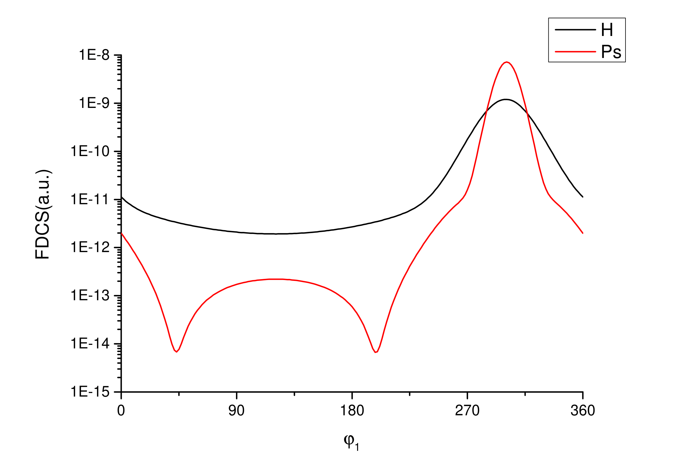
Figure 1: FDCS (a.u.) as a function of the electron scattering angle $\varphi_{1}$ in the case of ionization of the hydrogen atom H and positronium Ps. $\omega_{i}=5$ keV, $E_{e}=27.2$ eV, $\theta=\pi/3$.

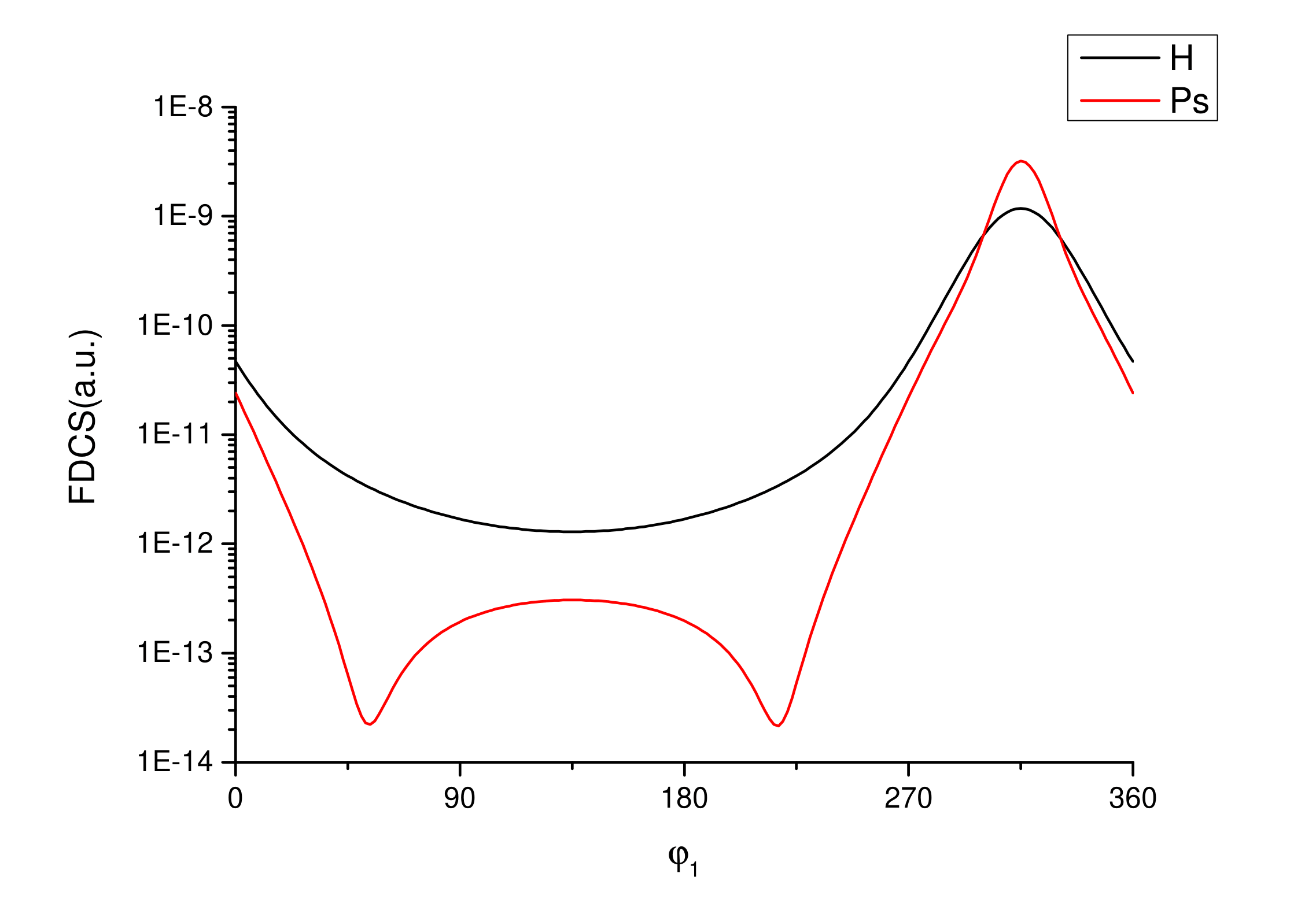
Figure 2: The same as in Fig. 4 for $\theta=\pi/2$.

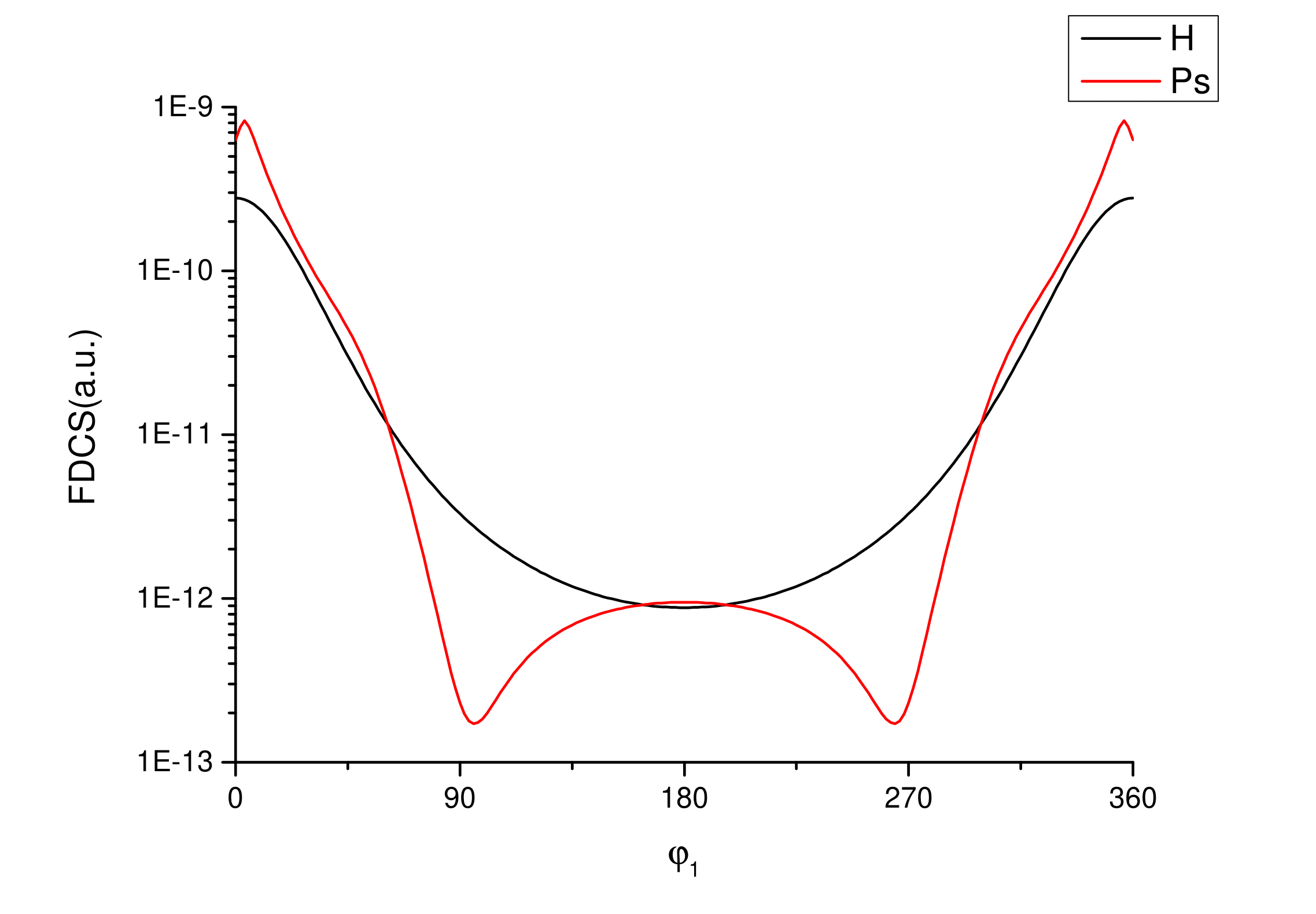
Figure 3: The same as in Fig. 4 for $\theta=\pi$.

Let us analyze Figs. 1 - 3, which show the total differential cross sections of the Compton ionization of the hydrogen atom and positronium. We should say, that in all calculations we found that the dependence on $t$ is quite weak, so we put everywhere $t=1$. First of all, we see the dominant peaks, when the angle $\beta$ between the vectors $\vec{p}_{1}$ and $\vec{Q}$ is equal to zero. In the theory of particle scattering, this peak is called the binary one and corresponds to the minimum of $|\vec{p}_{1}-\vec{Q}|$. This peak reflects a mechanism, when the entire transferred momentum is transferred to the electron, and the positron remains a ”spectator”.  Sufficiently flat second peak of the curve Ps is called the recoil peak in the theory of particle scattering. In this case, the value of $|\vec{p}_{1}-\vec{Q}|$ reaches its maximum, and the behavior of the cross section is determined mainly by the second term in (20), whose denominator does not depend on the angle $\beta$. In this region, the positron absorbs a $\gamma$-quantum, and the electron emits it during the disintegration. The transfer of energy from the positron to the electron occurs due to the Coulomb interaction of the particles in positronium. Such a process is possible, but unlikely, it is reflected in a very large ratio of the magnitudes of these peaks. In addition, the described process is secondary, and the electron escapes from the positronium isotropically, which is reflected in the ”flat” character of the backward peak. Thus, Figs. 1 - 3 present the main mechanisms of the Compton disintegration of positronium. It is interesting that, at a sufficiently high photon energy of 5 keV, the backward peak in hydrogen is not only absent, but turns into a minimum at the same place, where the Ps curve has the recoil peak. However, the structural differences between the curves are visible only on a logarithmic scale.

It should also be noted that the magnitude of the binary peak of the Ps curve slightly decreases, while the recoil peak slightly increases with increasing momentum transfer $Q$. This is due to an increase in the value of $|\vec{p}_{1}-\vec{Q}|$ for a fixed electron energy.

3.1 System of Coulomb resonances

Let us now consider the behavior of the cross section at the resonance, where the electron and positron fly parallel to each other with the same velocities. This happens, when the Coulomb number goes to infinity, $\zeta\to\infty$, or $\mu=|\vec{p}_{1}-\vec{Q}/2|\to 0.$ This is possible, when $\vec{p}_{1}\parallel\vec{Q}$, i.e. in the binary peak region, and for $p_{1}/k_{i}=\sin(\theta/2)<1$, if we set $t=1$ without loss of generality. In this case, it follows from Eq. (20)

$$\sum_{e_{i},e_{f}}|M|^{2}\approx\frac{1}{\mu}\ (1+\cos^{2}\theta)\frac{32\pi^{2}Z^{5}Q^{4}}{(Q^{2}/4+Z^{2})^{6}}\exp\left(-\ {\frac{2Z}{Q^{2}/4+Z^{2}}}\right).$$

As can be seen from (22), a pole appears in the cross section under the given kinematic conditions, which is characteristic of infinitely narrow dynamic resonances. However, this pole is not dangerous when integrating with respect to $d^{3}p_{1}$, since we make a change of variables and compensate this pole with the phase volume of the integration. However, let us assume that we need to integrate the FDCS over the photon scattering angle, for example, to calculate

$$DDCS_{\varphi_{1}}=\frac{d^{2}\sigma}{dE_{e}d\varphi_{1}}=2\pi\int_{0}^{\pi}\ \sin\theta\ d\theta\int_{0}^{2\pi}d\Phi\ FDCS.$$

This double differential cross section describes the angular and energy distribution of the electron for any direction of photon scattering. Let us ask ourselves a question, whether this integral will converge? To answer this question, we use expression (21) and write down the expression for $\mu^{2}$:

$$\mu^{2}=p^{2}_{1}-p_{1}Q\left(\cos\varphi_{1}\sin\frac{\theta}{2}-\sin\varphi_{1}\cos\frac{\theta}{2}\cos\Phi\right)+\frac{Q^{2}}{4}.$$

Recall that for $t=1$, $Q=2k_{i}\sin(\theta/2)$, and denote $\gamma=p_{1}/k$. Omitting intermediate calculations, we rewrite (24.1) in the form

$$\mu^{2}=k_{i}^{2}\left[\left(\gamma-\sin\frac{\theta}{2}\right)^{2}+2\gamma\sin\frac{\theta}{2}\left(1-\cos(\frac{\pi}{2}-\varphi_{1}-\frac{\theta}{2})\right)\right.\ +$$

$$\left.\gamma\sin\varphi_{1}\sin\theta(1+\cos\Phi)\frac{}{}\right].$$

All terms in (24.2) are positive, therefore $\mu=0$ if the conditions $\gamma=\sin(\theta_{0}/2),\ (\pi/2-\varphi_{1}-\theta_{0}/2)=0,\ (1+\cos\Phi_{0})=0$ are fulfilled simultaneously. Hence, in particular, it follows that $\gamma=\cos\varphi_{1}<1$. This is the condition, where one can expect a singularity in the FDCS. If $p_{1}>k_{i}$, or in our case $E_{e}>24.4$ eV, the singularities are absent.

Let us put $\theta=\theta_{0}+\delta$ and $\Phi=\pi-\lambda$ in (24.2), where the deviations $\lambda$ and $\delta$ are small. Then

$$\mu\approx k\sqrt{\frac{1}{4}\delta^{2}+\lambda^{2}\ \gamma^{2}(1-\gamma^{2})}.$$

and the FDCS is completely integrable in the neighborhood of the points $\theta=\theta_{0}$ and $\Phi=\pi$, if only $\gamma\neq 1$. However, in the phase volume of integral (23) in the vicinity of the point $\theta=\theta_{0}$ there is a factor $\sin\theta_{0}=2\gamma\sqrt{1-\gamma^{2}}$, which compensates this divergence. Thus, integral (23) converges, although numerical integration requires a certain accuracy in the vicinity of the zeros of expression (24.2).

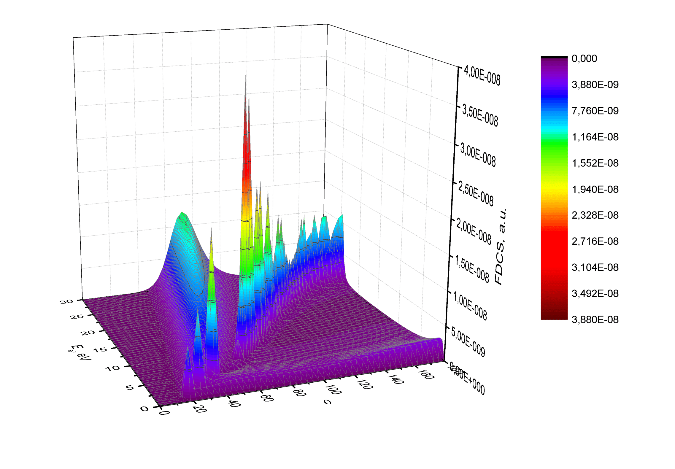
Figure 4: FDCS as a function of the photon scattering angle $\theta$ and the electron energy $E_{e}$ under the condition $\vec{p}_{1}\parallel\vec{Q}$. The value of $\mu$ is smoothed: $\mu\to\sqrt{\mu^{2}+\varepsilon^{2}},\ \varepsilon=0.01$. The line of resonances $\mu\sim 0$ is clearly visible.

Fig. 4 shows a 3D plot of the FDCS versus the electron energy and photon scattering angle in the binary peak region. It should be said right away that the angle $\beta$ itself depends on the scattering angles of the photon and the electron according to (21). Its fixation imposes a constraint on these observed angles. However, the resonance line is easily seen in the figure. The calculations were carried out while smoothing the singularity $\mu\to\sqrt{\mu^{2}+\varepsilon^{2}},\ \varepsilon=0.01$.

Let us discuss the above effect. In principle, a similar situation arises, when a hydrogen atom is ionized by a photon, if the final state is described by a Coulomb wave. Due to the difference between the masses of the proton and the electron, the singularity in the FDCS arises, when the electron energy tends to zero. This is precisely the energy boundary between the continuum and the spectrum of bound Coulomb states, which is sometimes called ”the Keldysh swamp”.  In this case, the size of the system tends to infinity. Formally, we are faced with an infinite number of thresholds of excitation reactions. As we can see, the matrix element (20.1) for the hydrogen ionization has a singularity at $p_{1}\to 0$. However, in the case of hydrogen, this pole is compensated by the factor $p_{1}$ in cross section (19.1), and the cross section tends to a constant as $p_{1}\to 0$.

The same situation takes place in positronium, only now the singularity depends on the angles. And there is a very simple condition for its occurrence $E_{e}=0.5(\omega_{i}/c)^{2}\sin^{2}(\theta/2)$. In this case, the electron and positron move parallel to each other with the same velocity, and they can be separated by any distance, including a rather large one. Formally, such a state can exist for an arbitrarily long time within the framework of non-relativistic physics, until a second photon is emitted (even with an energy close to zero), and the electron-positron pair again falls into a bound state. Thus, a resonance arises. An interesting question is: how to maintain such a state for as long as you like?

The described picture resembles the Thomas effect in the classical description of the capture of an electron by an ion from a target Thomas . That time there was no possibility to describe the bound state of the final atom in this effect, and it was described as the parallel motion of an electron and an ion with the same velocity. From this condition, the trajectory of the electron motion between heavy fragments was calculated, which gave a peak in the capture cross section (a second-order process in a quantum description) .

3.3 Double differential cross section

Now we consider the double differential cross sections, the measurements of which are easier. For example, in the case of cross section (23), we measure only the electron momentum. A 3D picture of this cross section for positronium is shown in Fig. 5. Here the photon energy is $\omega_{i}=3$ keV. First of all, it is striking that the cross section is noticeably different from zero at small angles of electron emission (forward scattering cone of the photon) and its low energies. The cross section goes to zero at $E_{e}\to 0$ in contrast to hydrogen, since there is no compensating pole here, which we wrote about above. This results in the sharp peak at low energies. Further, at small angles, two more peaks of different heights and widths stand out.

Let us consider these peaks in more detail in Figs. 6 – 8, where the same cross section is presented for the angle $\varphi_{1}=0$, but at different photon energies. These figures also show a similar slice of the cross section for the hydrogen atom.

Let us pay attention to the middle peak, which becomes discernible at the photon energy $\omega_{i}=5$  keV, but noticeably grows up as the photon energy decreases. It is easy to see that this peak appears at $p_{1}=k_{i}$, or $E_{e}=0.5(\omega_{i}/c)^{2}$. The origin of this peak has not been fully understood yet. It is not excluded that it is somehow related to the resonances discussed in the previous section, although it is difficult to reliably say about this after integration over the photon scattering angle. Hydrogen has nothing of this kind.

Let us discuss this peculiarity in the behavior of the cross section in more detail. In the theory of electron capture from a target and single ionization of the target by an ion at relatively low projectile and electron speeds, singularities are observed in the integral cross sections, when the electron and projectile velocities coincide. In the theory of capture, this is the above mentioned Thomas effect, while in the theory of ionization, this is the so-called ”shoulder” in the single differential cross section Schulz . It is observed quite well at proton energies of 75 keV and 100 keV. In our case, this is the coincidence of the electron and positron velocities after the disintegration of positronium by a photon. Thus, the assumption about the nature of the discussed peak is quite acceptable.

A wide peak at larger energies is observed for both positronium and hydrogen. The position of these peaks is also close to each other. Earlier in the study of hydrogen, it was found that the FDCS_H has a peak, when the electron takes over the entire transferred momentum, which corresponds to Compton scattering at a free electron. It seems that even after the integration over the angle of the scattered photon, this trend persists. Indeed, the peak is seen most clearly, when the photon is scattered into the backward cone, which leads to forward scattering of the electron. The integration over all angles smoothes the peak somehow, but does not override its physics. The presence of the light positron in positronium slightly changes the position and magnitude of this peak, but the physical effect remains the same.

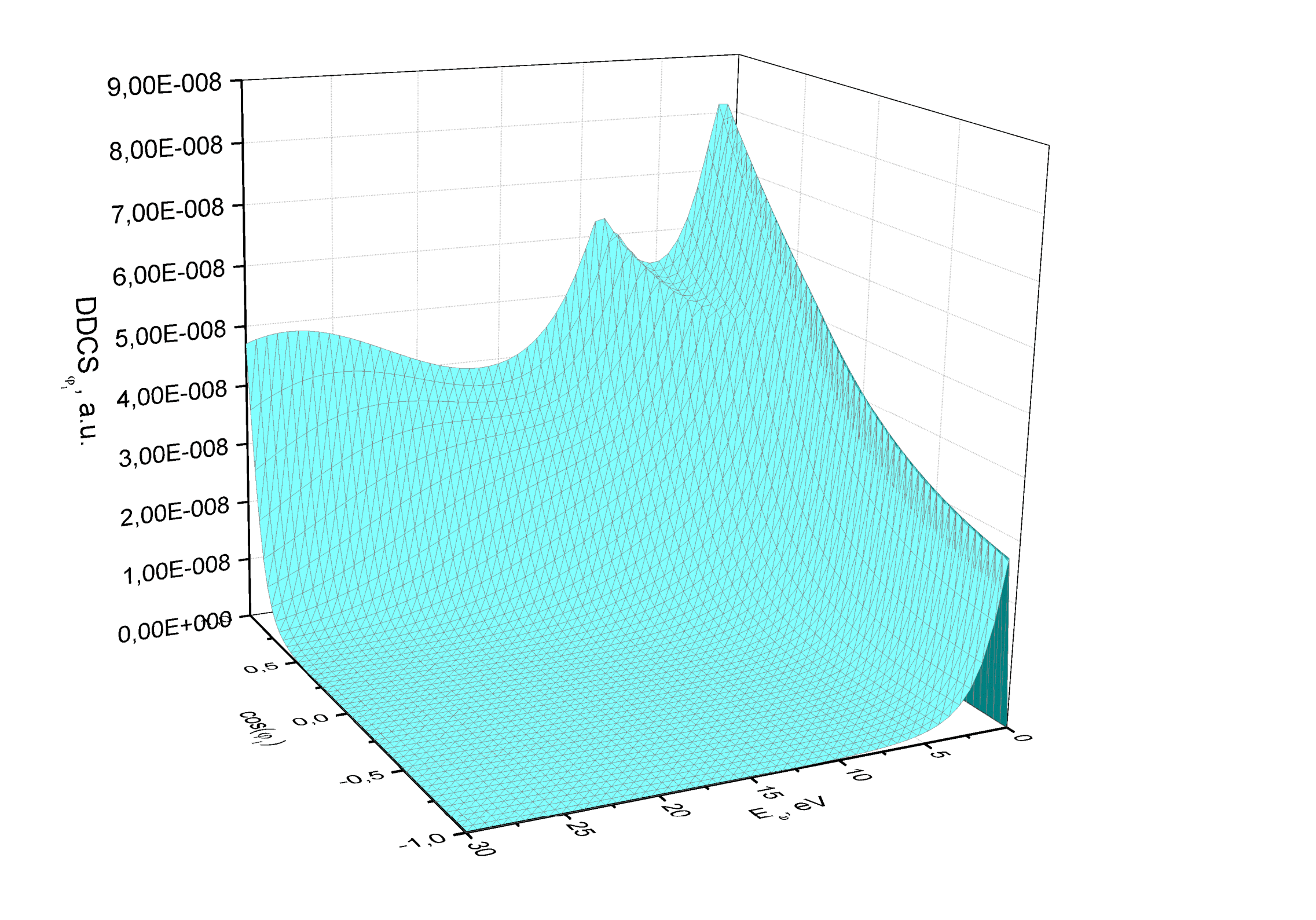
Figure 5: DDCS${}_{\varphi_{1}}$ (23) depending on the electron emission angle $\varphi_{1}$ and its energy $E_{e}$. The photon energy is $\omega_{i}=3\ keV$

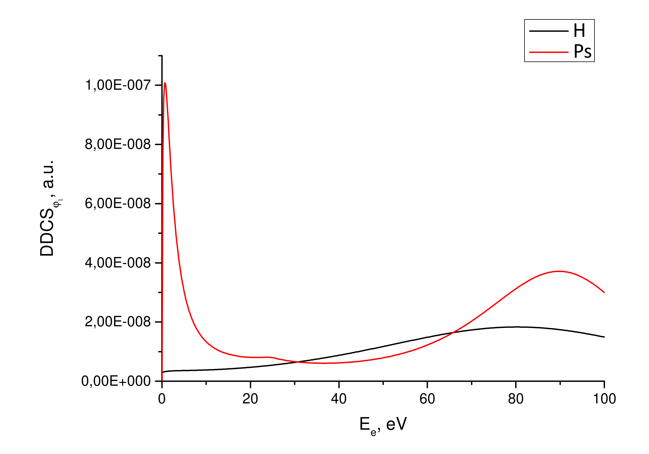
Figure 6: DDCS${}_{\varphi_{1}}$ (23) with the fixed angle $\varphi_{1}=0$. The photon energy is $\omega_{i}=5\ keV$. The red curve corresponds to positronium, the black curve corresponds to hydrogen.

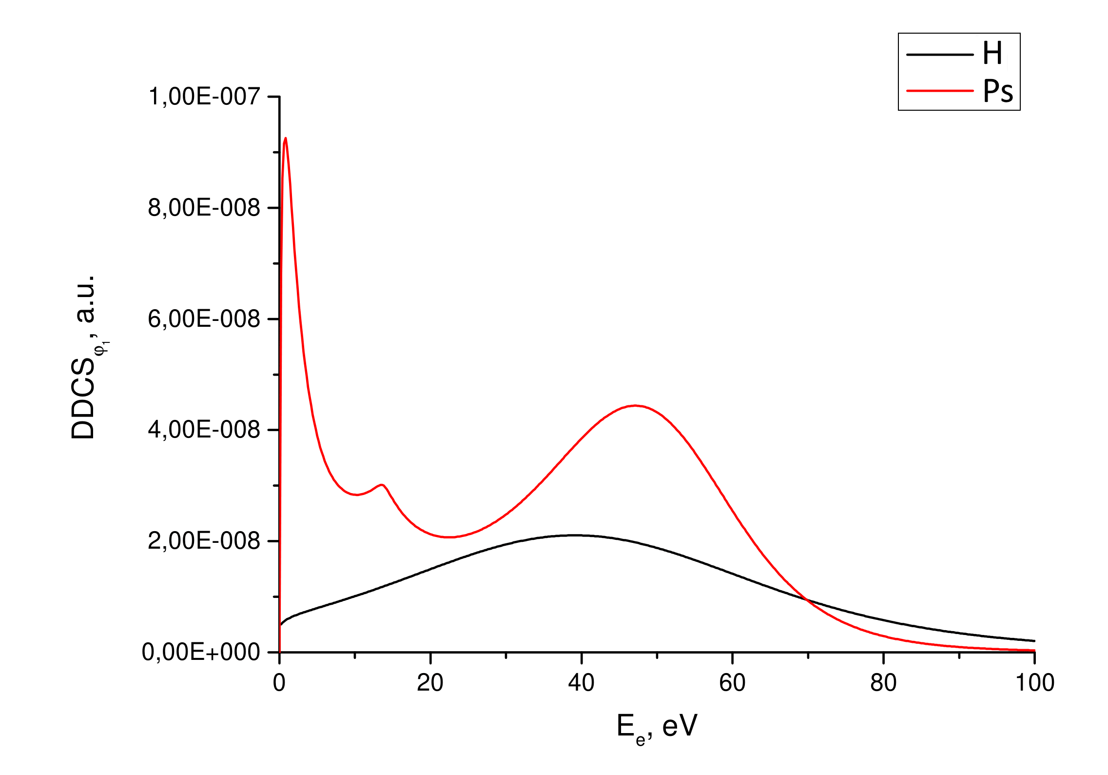
Figure 7: The same as in Fig. 6 for the photon energy $\omega_{i}=3.75\ keV$.

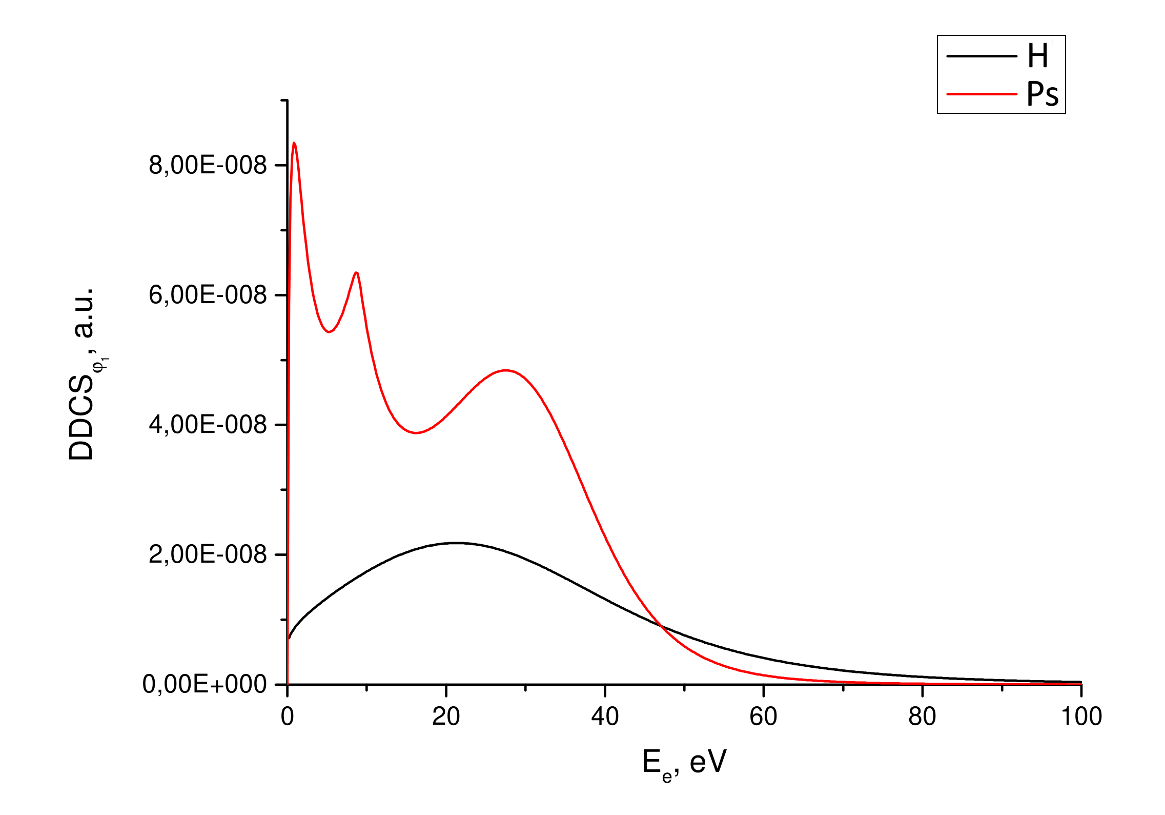
Figure 8: The same as in Fig. 6 for the photon energy $\omega_{i}=3\ keV$ .

4. CONCLUSION

We have considered the Compton disintegration of positronium in the non-relativistic approximation at a photon energy of several keV. A number of features are noted in the differential cross sections that distinguish the ionization (disintegration) of positronium from the ionization of the hydrogen atom. In particular, an interesting feature of the process are the resonances that arise in the parallel motion of the electron and positron with equal velocities after the disintegration. In hydrogen, only one such resonance state is observed in the total differential cross section at the energy of the emitted electron equal to zero. This is due to the use of the Coulomb function as the final state. For positronium, this point unfolds into a line of resonances at the electron energies $E_{e}=0.5(\omega_{i}/c)^{2}\sin^{2}(\theta/2)$. For the photon backscattering, the energy of the electron (and the positron), which is required to provide resonances, reaches its maximum value, after which the parallel motion of the electron and positron is no longer possible.

Author contribution statement

All authors contributed equally to the paper.

References

• (1) A.I.Akhiezer,V.B.Berestetskii, QuantumElectrodynamics (John Wiley and Sons, 1965), Β§30
• (2) S. Houamer, O. Chuluunbaatar, I.P. Volobuev, and Yu.V. Popov. ”Compton ionization of hydrogen atom near threshold by photons in the energy range of a few keV: Nonrelativistic approach” Eur.Phys.Journ.D 74 (2020), 81(9pp). https://doi.org/10.1140/epjd/e2020-100572-1
• (3) M. Kircher, F. Trinter, S. Grundmann, I. Vela-Perez, S. Brennecke, N. Eicke, J. Rist, S. Eckart, S. Houamer, O. Chuluunbaatar, Yu.V.Popov, I. P.Volobuev, Kai Bagschick, M.N. Piancastelli, M. Lein, T. Jahnke, M.S.SchΓΆffler, and R. DΓΆrner. ”Kinematically complete experimental study of Compton scattering at helium atoms near the threshold”, Nature Physics 16 (2020), 756 -760. https://doi.org/10.1038/s41567-020-0880-2
• (4) O. Chuluunbaatar, S. Houamer, Yu.V. Popov, I.P. Volobuev, M. Kircher, and R. Doerner. ”Compton ionization of atoms as a method of dynamical spectroscopy”, Journal of Quantitative Spectroscopy and Radiative Transfer (JQSRT) 272 (2021), 107820 (8pp) https://doi.org/10.1016/j.jqsrt.2021.107820
• (5) W. Bothe and H.Geiger, ”Uber das Wesen des Comptoneffekts; ein experimenteller Beitrag zur Theorie der Strahlung”. Z. Phys. 32 (1925), 639.
• (6) L.H. Thomas, ”On the capture of electrons by swiftly moving electrified particles”. Proc. R. Soc. Lond. 114 (1927), 561-578. https://www.jstor.org/stable/94828
• (7) M. Schulz et al, ”Absolute doubly differential single-ionizationcross sections in p+He collisions”, Phys. Rev.A 54 (1996), 2951. https://doi.org/10.1103/PhysRevA.54.2951