On the (In)Tractability of Reinforcement Learning for LTL Objectives

Abstract

In recent years, researchers have made significant progress in devising reinforcement-learning algorithms for optimizing linear temporal logic (LTL) objectives and LTL-like objectives. Despite these advancements, there are fundamental limitations to how well this problem can be solved. Previous studies have alluded to this fact but have not examined it in depth. In this paper, we address the tractability of reinforcement learning for general LTL objectives from a theoretical perspective. We formalize the problem under the probably approximately correct learning in Markov decision processes (PAC-MDP) framework, a standard framework for measuring sample complexity in reinforcement learning. In this formalization, we prove that the optimal policy for any LTL formula is PAC-MDP-learnable if and only if the formula is in the most limited class in the LTL hierarchy, consisting of formulas that are decidable within a finite horizon. Practically, our result implies that it is impossible for a reinforcement-learning algorithm to obtain a PAC-MDP guarantee on the performance of its learned policy after finitely many interactions with an unconstrained environment for LTL objectives that are not decidable within a finite horizon.

1 Introduction

In reinforcement learning, we situate an autonomous agent in an unknown environment and specify an objective. We want the agent to learn the optimal behavior for achieving the specified objective by interacting with the environment.

Specifying an Objective

The objective for the agent is a specification over possible trajectories of the overall system—the environment and the agent. Each trajectory is an infinite sequence of the states of the system, evolving through time. The objective specifies which trajectories are desirable so that the agent can identify optimal or near-optimal behaviors with respect to the objective.

The Reward Objective

One form of an objective is a reward function. A reward function specifies a scalar value, a reward, for each state of the system. The desired trajectories are those with higher cumulative discounted rewards. The reward-function objective is well studied (Sutton and Barto, 1998). It has desirable properties that allow reinforcement-learning algorithms to provide performance guarantees on learned behavior (Strehl et al., 2006), meaning that algorithms can guarantee learning behaviors that achieve almost optimal cumulative discounted rewards with high probability. Due to its versatility, researchers have adopted the reward-function objective as the de facto standard of behavior specification in reinforcement learning.

1.1 The Linear Temporal Logic Objective

However, reward engineering, the practice of encoding desirable behaviors into a reward function, is a difficult challenge in applied reinforcement learning (Dewey, 2014; Littman et al., 2017). To reduce the burden of reward engineering, linear temporal logic (LTL) has attracted researchers’ attention as an alternative objective.

LTL is a formal logic used initially to specify behaviors for system verification (Pnueli, 1977). An LTL formula is built from a set of propositions about the state of the environment, logical connectives, and temporal operators such as $\mathsf{G}\,$ (always) and $\mathsf{F}\,$ (eventually). Many reinforcement-learning tasks are naturally expressible with LTL (Littman et al., 2017). For some classic control examples, we can express: 1) Cart-Pole as $\mathsf{G}\,\mathit{up}$ (i.e., the pole always stays up), 2) Mountain-Car as $\mathsf{F}\,\mathit{goal}$ (i.e., the car eventually reaches the goal), and 3) Pendulum-Swing-Up as $\mathsf{F}\,\mathsf{G}\,\mathit{up}$ (i.e., the pendulum eventually always stays up).

Researchers have thus used LTL as an alternative objective specification for reinforcement learning  (Fu and Topcu, 2014; Sadigh et al., 2014; Li et al., 2017; Hahn et al., 2019; Hasanbeig et al., 2019; Bozkurt et al., 2020). Given an LTL objective specified by an LTL formula, each trajectory of the system either satisfies or violates that formula. The agent should learn the behavior that maximizes the probability of satisfying that formula. Moreover, research has shown that using LTL objectives supports automated reward shaping (Jothimurugan et al., 2019; Camacho et al., 2019; Jiang et al., 2020).

1.2 Trouble with Infinite Horizons

The general class of LTL objectives consists of infinite-horizon objectives—objectives that require inspecting infinitely many steps of a trajectory to determine if the trajectory satisfies the objective. For example, consider the objective $\mathsf{F}\,\mathit{goal}$ (eventually reach the goal). Given an infinite trajectory, the objective requires inspecting the entire trajectory in the worst case to determine that the trajectory violates the objective.

Despite the above developments on reinforcement learning with LTL objectives, the infinite-horizon nature of these objectives presents challenges that have been alluded to—but not formally treated—in prior work. Henriques et al. (2012); Ashok et al. (2019); Jiang et al. (2020) noted slow learning times for mastering infinite-horizon properties. Littman et al. (2017) provided a specific environment that illustrates the intractability of learning for a specific infinite-horizon objective, arguing for the use of a discounted variant of LTL.

A similar issue exists for the infinite-horizon, average-reward objectives. In particular, it is understood that reinforcement-learning algorithms do not have guarantees on the learned behavior for infinite-horizon, average-reward problems without additional assumptions on the environment (Kearns and Singh, 2002).

However, to our knowledge, no prior work has formally analyzed the learnability of LTL objectives.

Our Results

We leverage the PAC-MDP framework (Strehl et al., 2006) to prove that reinforcement learning for infinite-horizon LTL objectives is intractable. The intuition for this intractability is: Any finite number of interactions with an environment with unknown transition dynamics is insufficient to identify the environment dynamics perfectly. Moreover, for an infinite-horizon objective, a behavior’s satisfaction probability under the inaccurate environment dynamics can be arbitrarily different from the behavior’s satisfaction probability under the true dynamics. Consequently, a learner cannot guarantee with any confidence that it has identified near-optimal behavior for an infinite-horizon objective.

1.3 Implications for Relevant and Future Work

Our results provide a framework to categorize approaches that either focus on tractable LTL objectives or weaken the guarantees of an algorithm. As a result, we interpret several previous approaches as instantiations of the following categories:

• Work with finite-horizon LTL objectives, the complement of infinite-horizon objectives, to obtain guarantees on the learned behavior (Henriques et al., 2012). These objectives, like $a\land\mathsf{X}a$ ($a$ is true for two steps), are decidable within a known finite number of steps.

• Seek a best-effort confidence interval (Ashok et al., 2019). Specifically, the interval can be trivial in the worst case, denoting that learned behavior is a maximally poor approximation of the optimal behavior.

• Make additional assumptions about the environment to obtain guarantees on the learned behavior (Fu and Topcu, 2014; Brázdil et al., 2014).

• Change the problem by working with LTL-like objectives such as: 1. relaxed LTL objectives that become exactly LTL in the (unreachable) limit (Sadigh et al., 2014; Hahn et al., 2019; Hasanbeig et al., 2019; Bozkurt et al., 2020) and 2. objectives that use temporal operators but employ a different semantics (Littman et al., 2017; Li et al., 2017; Giacomo et al., 2019; Camacho et al., 2019). The learnability of these objectives is a potential future research direction.

1.4 Contributions

We make the following contributions:

• A formalization of reinforcement learning with LTL objectives under the probably approximately correct in Markov decision processes (PAC-MDP) framework (Fiechter, 1994; Kearns and Singh, 2002; Kakade, 2003), a standard framework for measuring sample complexity for reinforcement-learning algorithms; and a formal definition of LTL-PAC-learnable, a learnability criterion for LTL objectives.

• A statement and proof that: 1. Any infinite-horizon LTL formula is not LTL-PAC-learnable. 2. Any finite-horizon LTL formula is LTL-PAC-learnable. To that end, for any infinite-horizon formula, we give a construction of two special families of MDPs as counterexamples with which we prove that the formula is not LTL-PAC-learnable.

• Experiments with current reinforcement-learning algorithms for LTL objectives that provide empirical support for our theoretical result.

• A categorization of approaches that focus on tractable objectives or weaken the guarantees of LTL-PAC-learnable and a classification of previous approaches into these categories.

2 Preliminaries: Reinforcement Learning

This section provides definitions for MDPs, planning, reinforcement learning, and PAC-MDP.

2.1 Markov Processes

We first review some basic notations for Markov processes.

A Markov decision process (MDP) is a tuple $\mathcal{M}=(S,A,P,s_{0})$, where $S$ and $A$ are finite sets of states and actions, $P\colon(S\times A)\to\Delta\left(S\right)$ is a transition probability function that maps a current state and an action to a distribution over next states, and $s_{0}\in S$ is an initial state. The MDP is sometimes referred to as the environment MDP to distinguish it from any specific objective.

A (stochastic) Markovian policy $\pi$ for an MDP is a function $\pi\colon S\to\Delta\left(A\right)$ that maps each state of the MDP to a distribution over the actions.

A (stochastic) non-Markovian policy $\pi$ for an MDP is a function $\pi\colon(\left(S\times A\right)^{*}\times S)\to\Delta\left(A\right)$ that maps a history of states and actions of the MDP to a distribution over actions.

An MDP and a policy on the MDP induce a discrete-time Markov chain (DTMC). A DTMC is a tuple $\mathcal{D}=(S,P,s_{0})$, where $S$ is a finite set of states, $P\colon S\to\Delta\left(S\right)$ is a transition-probability function that maps a current state to a distribution over next states, and $s_{0}\in S$ is an initial state. A sample path of $\mathcal{D}$ is an infinite sequence of states $w\in S^{\upomega}$. The sample paths of a DTMC form a probability space.

2.2 Objective

An objective for an MDP $\mathcal{M}=(S,A,P,s_{0})$ is a measurable function $\kappa\colon S^{\upomega}\to\mathbb{R}$ on the probability space of the DTMC $\mathcal{D}$ induced by $\mathcal{M}$ and a policy $\pi$. The value of the objective for the MDP $\mathcal{M}$ and a policy $\pi$ is the expectation of the objective under that probability space:

$$V^{\pi}_{\mathcal{M},\kappa}=\mathsf{E}_{#1}\left[\kappa(w)\right]\quad(\mathcal{D}\text{ induced by }\mathcal{M}\text{ and }\pi).$$

For example, the cumulative discounted rewards objective (Puterman, 1994) with discount $\gamma$ and a reward function $R\colon S\to\mathbb{R}$ is: $\kappa^{\text{reward}}(w)\triangleq\sum_{i=0}^{\infty}\gamma^{i}\cdot R(w[i]).$

An optimal policy maximizes the objective’s value: $\pi^{*}=\operatorname*{arg\,max}_{\pi}V^{\pi}_{\mathcal{M},\kappa}$. The optimal value $V^{\pi^{*}}_{\mathcal{M},\kappa}$ is then the objective value of the optimal policy. A policy $\pi$ is $\epsilon$-optimal if its value is $\epsilon$-close to the optimal value: $V^{\pi}_{\mathcal{M},\kappa}\geq V^{\pi^{*}}_{\mathcal{M},\kappa}-\epsilon$.

2.3 Planning with a Generative Model

A planning-with-generative-model algorithm (Kearns et al., 1999; Grill et al., 2016) has access to a generative model, a sampler, of an MDP’s transitions but does not have direct access to the underlying probability values. It can take any state and action and sample a next state. It learns a policy from those sampled transitions.

Formally, a planning-with-generative-model algorithm $\mathcal{A}$ is a tuple $(\mathcal{A}^{\text{S}},\mathcal{A}^{\text{L}})$, where $\mathcal{A}^{\text{S}}$ is a sampling algorithm that drives how the environment is sampled, and $\mathcal{A}^{\text{L}}$ is a learning algorithm that learns a policy from the samples obtained by applying the sampling algorithm.

In particular, the sampling algorithm $\mathcal{A}^{\text{S}}$ is a function that maps from a history of sampled environment transitions $((s_{0},a_{0},s^{\prime}_{0})\dots(s_{k},a_{k},s^{\prime}_{k}))$ to the next state and action to sample $(s_{k+1},a_{k+1})$ , resulting in $\mathsf{s}_{k+1}^{\prime}\sim\mathsf{P}_{#1}\left(\nonscript\,\cdot\nonscript\;\middle|\nonscript\>\allowbreak s_{k+1},a_{k+1}\nonscript\,\right)$. Iterative application of the sampling algorithm $\mathcal{A}^{\text{S}}$ produces a sequence of sampled environment transitions.

The learning algorithm is a function that maps that sequence of sampled environment transitions to a non-Markovian policy of the environment MDP. Note that the sampling algorithm can internally consider alternative policies as part of its decision of what to sample. Also, note that we deliberately consider non-Markovian policies since the optimal policy for an LTL objective (defined later) is non-Markovian in general (unlike a cumulative discounted rewards objective).

2.4 Reinforcement Learning

In reinforcement learning, an agent is situated in an environment MDP and only observes state transitions. We also allow the agent to reset to the initial state as in Fiechter (1994).

We can view a reinforcement-learning algorithm as a special kind of planning-with-generative-model algorithm $(\mathcal{A}^{\text{S}},\mathcal{A}^{\text{L}})$ such that the sampling algorithm always either follows the next state sampled from the environment or resets to the initial state of the environment.

2.5 Probably Approximately Correct in MDPs

A successful planning-with-generative-model algorithm (or reinforcement-learning algorithm) should learn from the sampled environment transitions and produce an optimal policy for the objective in the environment MDP. However, since the environment transitions may be stochastic, we cannot expect an algorithm to always produce the optimal policy. Instead, we seek an algorithm that, with high probability, produces a nearly optimal policy. The PAC-MDP framework (Fiechter, 1994; Kearns and Singh, 2002; Kakade, 2003), which takes inspiration from probably approximately correct (PAC) learning (Valiant, 1984), formalizes this notion. The PAC-MDP framework requires efficiency in both sampling and algorithmic complexity. In this work, we only consider sample efficiency and thus omit the requirement on algorithmic complexity. Next, we generalize the PAC-MDP framework from reinforcement-learning with a reward objective to planning-with-generative-model with a generic objective.

Definition 1.

Given an objective $\kappa$, a planning-with-generative-model algorithm $(\mathcal{A}^{\text{S}},\mathcal{A}^{\text{L}})$ is $\kappa$-PAC (probably approximately correct for objective $\kappa$) in an environment MDP $\mathcal{M}$ if, with the sequence of transitions $T$ of length $N$ sampled using the sampling algorithm $\mathcal{A}^{\text{S}}$, the learning algorithm $\mathcal{A}^{\text{L}}$ outputs a non-Markovian $\epsilon$-optimal policy with probability at least $1-\delta$ for any given $\epsilon>0$ and $0<\delta<1$. That is:

$$\mathsf{P}_{#1}\left(V^{\mathcal{A}^{\text{L}}\left(T\right)}_{\mathcal{M},\kappa}\geq V^{\pi^{*}}_{\mathcal{M},\kappa}-\epsilon\right)\geq 1-\delta.$$ (1)

We use $\mathsf{T}{\sim}\left\langle\mathcal{M},\mathcal{A}^{\text{S}}\right\rangle_{N}$to denote that the probability space is over the set of length-$N$ transition sequences sampled from the environment $\mathcal{M}$ using the sampling algorithm $\mathcal{A}^{\text{S}}$. For brevity, we will drop $\left\langle\mathcal{M},\mathcal{A}^{\text{S}}\right\rangle_{N}$ when it is clear from context and simply write $\mathsf{P}_{#1}(.)$ to denote that the probability space is over the sampled transitions.

Definition 2.

Given an objective $\kappa$, a $\kappa$-PAC planning-with-generative-model algorithm is sample efficiently $\kappa$-PAC if the number of sampled transitions $N$ is asymptotically polynomial in $\frac{1}{\epsilon}$, $\frac{1}{\delta}$, $|S|$, $|A|$.

Note that the definition allows the polynomial to have constant coefficients that depends on $\kappa$.

3 Linear Temporal Logic Objectives

This section describes LTL and its use in objectives.

3.1 Linear Temporal Logic

A linear temporal logic (LTL) formula is built from a finite set of atomic propositions $\Pi$, logical connectives $\neg,\land,\lor$, temporal next $\mathsf{X}$, and temporal operators $\mathsf{G}\,$ (always), $\mathsf{F}\,$ (eventually), and $\mathbin{\mathsf{U}}$ (until). Equation 2 gives the grammar of an LTL formula $\phi$ over the set of atomic propositions $\Pi$:

$$\phi\mathrel{\hbox to0.0pt{\raisebox{1.29167pt}{$\cdot$}\hss}\raisebox{-1.29167pt}{$\cdot$}}=a\>\big{|}\>\neg\phi\>\big{|}\>\phi\land\phi\>\big{|}\>\phi\lor\phi\>\big{|}\>\mathsf{X}\phi\>\big{|}\>\mathsf{G}\,\phi\>\big{|}\>\mathsf{F}\,\phi\>\big{|}\>\phi\mathbin{\mathsf{U}}\phi,\;a\in\Pi.$$ (2)

LTL is a logic over infinite-length words. Informally, these temporal operators have the following meanings: $\mathsf{X}\phi$ asserts that $\phi$ is true at the next time step; $\mathsf{G}\,\phi$ asserts that $\phi$ is always true; $\mathsf{F}\,\phi$ asserts that $\phi$ is eventually true; $\psi\mathbin{\mathsf{U}}\phi$ asserts that $\psi$ needs to stay true until $\phi$ eventually becomes true. We give the formal semantics of each operator in LABEL:sec:ltl-hierarchy-full. We write $w\vDash\phi$ to denote that the infinite word $w$ satisfies $\phi$.

3.2 MDP with LTL Objectives

An LTL objective maximizes the probability of satisfying an LTL formula. We formalize this notion below.

An LTL specification for an MDP is a tuple $(\mathcal{L},\phi)$, where $\mathcal{L}\colon S\to 2^{\Pi}$ is a labeling function, and $\phi$ is an LTL formula over atomic propositions $\Pi$. The labeling function is a classifier mapping each MDP state to a tuple of truth values of the atomic propositions in $\phi$. For a sample path $w$, we use $\mathcal{L}\left(w\right)$ to denote the element-wise application of $\mathcal{L}$ on $w$.

The LTL objective $\xi$ specified by the LTL specification is the satisfaction of the formula $\phi$ of a sample path mapped by the labeling function $\mathcal{L}$, that is: $\kappa(w)\triangleq\mathbb{1}_{\mathcal{L}(w)\vDash\phi}$. The value of this objective is called the satisfaction probability of $\xi$:

$$V^{\pi}_{\mathcal{M},\xi}=\mathsf{P}_{#1}\left(\mathcal{L}\left(w\right)\vDash\phi\right)\quad(\mathcal{D}\text{ induced by }\mathcal{M}\text{ and }\pi).$$

3.3 Infinite Horizons in LTL Objectives

Figure 1: The hierarchy of LTL

An LTL formula describes either a finite-horizon or infinite-horizon property. Manna and Pnueli (1987) classified LTL formulas into seven classes, as shown in Figure 1. Each class includes all the classes to the left of that class (e.g., $\mathit{{Finitary}}\,{\subset}\,\mathit{{Guarantee}}$, but $\mathit{{Safety}}\,{\not\subset}\,\mathit{{Guarantee}}$), with the $\mathit{{Finitary}}$ class being the most restricted and the $\mathit{{Reactivity}}$ class being the most general. Below we briefly describe the key properties of the leftmost three classes relevant to the core of this paper. We present a complete description of all the classes in LABEL:sec:ltl-hierarchy-full.

• $\phi\,{\in}\,\mathit{{Finitary}}$ iff there exists a horizon $H$ such that infinite-length words sharing the same prefix of length $H$ are either all accepted or all rejected by $\phi$. E.g., $a\land\mathsf{X}a$ (i.e., $a$ is true for two steps) is in $\mathit{{Finitary}}$.

• $\phi\,{\in}\,\mathit{{Guarantee}}$ iff there exists a language of finite words $L$ (i.e., a Boolean function on finite-length words) such that $w\vDash\phi$ if $L$ accepts a prefix of $w$. Informally, a formula in $\mathit{{Guarantee}}$ asserts that something eventually happens. E.g., $\mathsf{F}\,a$ (i.e., eventually $a$ is true) is in $\mathit{{Guarantee}}$.

• $\phi\,{\in}\,\mathit{{Safety}}$ iff there exists a language of finite words $L$ such that $w\vDash\phi$ if $L$ accepts all prefixes of $w$. Informally, a formula in $\mathit{{Safety}}$ asserts that something always happens. E.g., $\mathsf{G}\,a$ (i.e., $a$ is always true) is in $\mathit{{Safety}}$.

Moreover, the set of finitary is the intersection of the set of guarantee formulas and the set of safety formulas. Any $\phi\,{\in}\,\mathit{{Finitary}}$, or equivalently $\phi\,{\in}\,\mathit{{Guarantee}}\cap\mathit{{Safety}}$, inherently describes finite-horizon properties. Any $\phi\,{\not\in}\,\mathit{{Finitary}}$, or equivalently $\phi\,{\in}\,\mathit{{Guarantee}}^{\complement}\cup\mathit{{Safety}}^{\complement}$, inherently describes infinite-horizon properties. We will show that reinforcement-learning algorithms cannot provide PAC guarantees for LTL objectives specified by formulas that describe infinite-horizon properties.

3.4 Intuition of the Problem

Figure 2: Two MDPs parameterized by $p$ in range $0<p<1$. Action $a_{1}$ in the MDP on the left and action $a_{2}$ in the MDP on the right have probability $p$ of transitioning to the state $h$. Conversely, action $a_{2}$ in the MDP on the left and action $a_{1}$ in the MDP on the right have probability $p$ of transitioning to the state $q$. Both actions in both MDPs have probability $1-p$ to loop around the state $g$.

Suppose that we send an agent into one of the MDPs in Figure 2, and want its behavior to satisfy “eventually reach the state $h$”, expressed as the LTL formula $\mathsf{F}\,h$. The optimal behavior is to always choose the action along the transition $g\rightarrow h$ for both MDPs (i.e., $a_{1}$ for the MDP on the left and $a_{2}$ for the MDP on the right). This optimal behavior satisfies the objective with probability one. However, the agent does not know which of the two MDPs it is in. The agent must follow its sampling algorithm to explore the MDP’s dynamics and use its learning algorithm to learn this optimal behavior.

If the agent observes neither transitions going out of $g$ (i.e., $g\rightarrow h$ or $g\rightarrow q$) during sampling, it will not be able to distinguish between the two actions. The best it can do is a 50% chance guess and cannot provide any non-trivial guarantee on the probability of learning the optimal action.

On the other hand, if the agent observes one of the transitions going out of $g$, it will be able to determine which action leads to state $h$, thereby learning always to take that action. However, the probability of observing any such transition with $N$ interactions is at most $1-(1-p)^{N}$. This is problematic: with any finite $N$, there always exists a value of $p$ such that this probability is arbitrarily close to $0$. In other words, with any finite number of interactions, without knowing the value of $p$, the agent cannot guarantee (a non-zero lower bound on) its chance of learning a policy that satisfies the LTL formula $\mathsf{F}\,h$.

Further, the problem is not limited to this formula. For example, the objective “never reach the state $q$”, expressed as the formula $\mathsf{G}\,\neg q$, has the same problem in these two MDPs. More generally, for any LTL formula describing an infinite-horizon property, we construct two counterexample MDPs with the same nature as the ones in Figure 2, and prove that it is impossible to guarantee learning the optimal policy.

4 Learnability of LTL Objectives

Figure 3: Counterexample MDPs $\mathcal{M}_{1}$ and $\mathcal{M}_{2}$, with transitions distinguished by arrow types (see legend). Both MDPs are parameterized by the parameter $p$ that is in range $0<p<1$. Unlabeled edges are deterministic (actions $a_{1}$ and $a_{2}$ transition with probability $1$). Ellipsis indicates a deterministic chain of states.

This section states and outlines the proof to the main result.

By specializing the $\kappa$-PAC definitions (Definitions 1 and 2) with the definition of LTL objectives in Section 3.2, we obtain the following definitions of LTL-PAC.

Definition 3.

Given an LTL objective $\xi$, a planning-with-generative-model algorithm $(\mathcal{A}^{\text{S}},\mathcal{A}^{\text{L}})$ is LTL-PAC (probably approximated correct for LTL objective $\xi$) in an environment MDP $\mathcal{M}$ for the LTL objective $\xi$ if, with the sequence of transitions $T$ of length $N$ sampled using the sampling algorithm $\mathcal{A}^{\text{S}}$, the learning algorithm $\mathcal{A}^{\text{L}}$ outputs a non-Markovian $\epsilon$-optimal policy with a probability of at least $1-\delta$ for all $\epsilon>0$ and $0<\delta<1$. That is,

$$\mathsf{P}_{#1}\left(V^{\mathcal{A}^{\text{L}}\left(T\right)}_{\mathcal{M},\xi}\geq V^{\pi^{*}}_{\mathcal{M},\xi}-\epsilon\right)\geq 1-\delta.$$ (3)

We call the probability on the left of the inequality the LTL-PAC probability of the algorithm $(\mathcal{A}^{\text{S}},\mathcal{A}^{\text{L}})$.

Definition 4.

Given an LTL objective $\xi$, an LTL-PAC planning-with-generative-model algorithm for $\xi$ is sample efficiently LTL-PAC if the number of sampled transitions $N$ is asymptotically polynomial to $\frac{1}{\epsilon}$, $\frac{1}{\delta}$, $|S|$, $|A|$.

With the above definitions, we can now define the PAC learnability of an LTL objective and state the main theorem.

Definition 5.

An LTL formula $\phi$ over atomic propositions $\Pi$ is LTL-PAC-learnable by planning-with-generative-model (reinforcement-learning) if there exists a sample efficiently LTL-PAC planning-with-generative-model (reinforcement-learning) algorithm for all environment MDPs and all consistent labeling functions $\mathcal{L}$ (that is, $\mathcal{L}$ maps from the MDP’s states to $2^{\Pi}$) for the LTL objective specified by $(\mathcal{L},\phi)$.

Theorem 1.

An LTL formula $\phi$ is LTL-PAC-learnable by reinforcement-learning (planning-with-generative-model) if (and only if) $\phi$ is finitary.

Between the two directions of Theorem 1, the forward direction (“only if”) is more important. The forward direction states that for any LTL formula not in $\mathit{{Finitary}}$ (that is, infinite-horizon properties), there does not exist a planning-with-generative-model algorithm—which by definition also excludes any reinforcement-learning algorithm—that is sample efficiently LTL-PAC for all environments. This result is the core contribution of the paper—infinite-horizon LTL formulas are not sample efficiently LTL-PAC-learnable.

Alternatively, the reverse direction of Theorem 1 states that, for any finitary formula (finite-horizon properties), there exists a reinforcement-learning algorithm—which by definition is also a planning-with-generative-model algorithm—that is sample efficiently LTL-PAC for all environments.

4.1 Proof of Theorem 1: Forward Direction

This section proves the forward direction of Theorem 1. First, we construct a family of pairs of MDPs. Then, for the singular case of the LTL formula $\mathsf{F}\,h_{0}$, we derive a sample complexity lower bound for any LTL-PAC planning-with-generative-model algorithm applied to our family of MDPs. This lower bound necessarily depends on a specific transition probability in the MDPs. Finally, we generalize this bound to any non-finitary LTL formula and conclude the proof.

4.1.1 MDP Family

We give two constructions of parameterized counterexample MDPs $\mathcal{M}_{1}$ and $\mathcal{M}_{2}$ shown in Figure 3. The key design behind each pair in the family is that no planning-with-generative-model algorithm can learn a policy that is simultaneously $\epsilon$-optimal on both MDPs without observing a number of samples that depends on the probability of a specific transition.

Both MDPs are parameterized by the shape parameters $k$, $l$, $u$, $v$, $m$, $n$, and an unknown transition probability parameter $p$. The actions are $\{a_{1},a_{2}\}$, and the state space is partitioned into three regions (as shown in Figure 3: states $g_{0\dots l}$ (the grey states), states $h_{0\dots v}$ (the line-hatched states), and states $q_{0\dots n}$ (the white states). All transitions, except $g_{l}\rightarrow h_{0}$ and $g_{l}\rightarrow q_{0}$, are the same between $\mathcal{M}_{1}$ and $\mathcal{M}_{2}$. The effect of this difference between the two MDPs is that, for $\mathcal{M}_{i}$, $i\in\{1,2\}$:

• Action $a_{i}$ in $\mathcal{M}_{i}$ at the state $g_{l}$ will transition to the state $h_{0}$ with probability $p$, inducing a run that cycles in the region $h_{u\dots v}$ forever.

• Action $a_{3-i}$ (the alternative to $a_{i}$) in $\mathcal{M}_{i}$ at the state $g_{l}$ will transition to the state $q_{0}$ with probability $p$, inducing a run that cycles in the region $q_{m\dots n}$ forever.

Further, for any policy, a run of the policy on both MDPs must eventually reach $h_{0}$ or $q_{0}$ with probability $1$, and ends in an infinite cycle in either $h_{u\dots v}$ or $q_{m\dots n}$.

4.1.2 Sample Complexity of $\mathsf{F}\,h_{0}$

We next consider the LTL objective $\xi^{h_{0}}$ specified by the LTL formula $\mathsf{F}\,h_{0}$ and the labeling function $\mathcal{L}^{h_{0}}$ that labels only the state $h_{0}$ as $\mathit{true}$. A sample path on the MDPs (Figure 3) satisfies this objective iff the path reaches the state $h_{0}$.

Given $\epsilon>0$ and $0<\delta<1$, our goal is to derive a lower bound on the number of sampled environment transitions performed by an algorithm, so that the satisfaction probability of $\pi$, the learned policy, is $\epsilon$-optimal (i.e., $V^{\pi}_{\mathcal{M},\xi^{h_{0}}}\geq V^{\pi^{*}}_{\mathcal{M},\xi^{h_{0}}}-\epsilon$) with a probability of least $1-\delta$.

The key rationale behind the following lemma is that, if a planning-with-generative-model algorithm has not observed any transition to either $h_{0}$ or $q_{0}$, the learned policy cannot be $\epsilon$-optimal in both $\mathcal{M}_{1}$ and $\mathcal{M}_{2}$.

Lemma 2.

For any planning-with-generative-model algorithm $(\mathcal{A}^{\text{S}},\mathcal{A}^{\text{L}})$, it must be the case that: $\min\left(\zeta_{1},\zeta_{2}\right)\leq\frac{1}{2}$, where $\zeta_{i}=\mathsf{P}_{#1}\left(\nonscript\,V^{\mathcal{A}^{\text{L}}(T)}_{\mathcal{M}_{i},\xi^{h_{0}}}\geq V^{\pi^{*}}_{\mathcal{M}_{i},\xi^{h_{0}}}-\epsilon\nonscript\;\middle|\nonscript\>\allowbreak n\left(T\right)=0\nonscript\,\right)$ and $n(T)$ is the number of transitions in $T$ that start from $g_{l}$ and end in either $h_{0}$ or $q_{0}$.

The value $\zeta_{i}$ is the LTL-PAC probability of a learned policy on $\mathcal{M}_{i}$, given that the planning-with-generative-model algorithm did not observe any information that allows the algorithm to distinguish between $\mathcal{M}_{1}$ and $\mathcal{M}_{2}$.

Proof.

We present a proof of Lemma 2 in LABEL:sec:proofofminofm1m2pacprob. ∎

A planning-with-generative-model algorithm cannot learn an $\epsilon$-optimal policy without observing a transition to either $h_{0}$ or $q_{0}$. Therefore, we bound the sample complexity of the algorithm from below by the probability that the sampling algorithm does observe such a transition:

Lemma 3.

For the LTL objective $\xi^{h_{0}}$, the number of samples, $N$, for an LTL-PAC planning-with-generative-model algorithm for both $\mathcal{M}_{1}$ and $\mathcal{M}_{2}$ (for any instantiation of the parameters $k,l,u,v,m,n$) has a lower bound of $N\geq\frac{\log(2\delta)}{\log\left(1-p\right)}$.

Below we give a proof sketch of Lemma 3; we give the complete proof in LABEL:sec:ltlpaclowerboundFh0fullproof.

Proof Sketch of Lemma 3.

First, we assert that the two inequalities of Equation 3 for both $\mathcal{M}_{1}$ and $\mathcal{M}_{2}$ holds true for a planning-with-generative-model algorithm. Next, by conditioning on $n(T)=0$, plugging in the notation of $\zeta_{i}$, and relaxing both inequalities, we get $(1-\zeta_{i})\mathsf{P}_{#1}(n(T)=0)\leq\delta$, for $i\in\{1,2\}$. Then, since $n(T)=0$ only occurs when all transitions from $g_{l}$ end in $g_{k}$, we have $\mathsf{P}_{#1}(n(T)=0)\geq(1-p)^{N}$. Combining the inequalities, we get $(1-\min(\zeta_{1},\zeta_{2}))(1-p)^{N}\leq\delta$. Finally, we apply Lemma 2 to get the desired lower bound of $N\,{\geq}\,\frac{\log(2\delta)}{\log(1-p)}$. ∎

4.1.3 Sample Complexity of Non-finitary Formulas

This section generalizes our lower bound on $\mathsf{F}\,h_{0}$ to all non-finitary LTL formulas. The key observation is that for any non-finitary LTL formula, we can choose a pair of MDPs, $\mathcal{M}_{1}$ and $\mathcal{M}_{2}$, from our MDP family. For both MDPs in this pair, finding an $\epsilon$-optimal policy for $\mathsf{F}\,h_{0}$ is reducible to finding an $\epsilon$-optimal policy for the given formula. By this reduction, the established lower bound for the case of $\mathsf{F}\,h_{0}$ also applies to the case of any non-finitary formula. Therefore, the sample complexity of learning an $\epsilon$-optimal policy for any non-finitary formula has a lower bound of $\frac{\log(2\delta)}{\log\left(1-p\right)}$.

We will use $[w_{1};w_{2};\dots w_{n}]$ to denote the concatenation of the finite-length words $w_{1}\dots w_{n}$. We will use $w^{i}$ to denote the repetition of the finite-length word $w$ by $i$ times, and $w^{\infty}$ to denote the infinite repetition of $w$.

Definition 6.

An accepting (resp. rejecting) infinite-length word $[w_{a};w_{b}^{\infty}]$ of $\phi$ is uncommittable if there exists finite-length words $w_{c}$, $w_{d}$ such that $\phi$ rejects (resp. accepts) $[w_{a};w_{b}^{i};w_{c};w_{d}^{\infty}]$ for all $i\in\mathbb{N}$.

Lemma 4.

If $\phi$ has an uncommittable word $w$, there is an instantiation of $\mathcal{M}_{1}$ (or $\mathcal{M}_{2}$) in Figure 3 and a labeling function $\mathcal{L}$, such that, for any policy, the satisfaction probabilities of that policy in $\mathcal{M}_{1}$ (or $\mathcal{M}_{2}$) for the LTL objectives specified by $(\mathcal{L},\phi)$ and $(\mathcal{L}^{h_{0}},\mathsf{F}\,h_{0})$ are the same.

Proof.

For an uncommittable word $w$, we first find the finite-length words $w_{a}$,$w_{b}$,$w_{c}$,$w_{d}$ according to Definition 6. We then instantiate $\mathcal{M}_{1}$ and $\mathcal{M}_{2}$ in Figure 3 as follows.

• If $w$ is an uncommittable accepting word, we set $k$, $l$, $u$, $v$, $m$, $n$ (Figure 3) to $|w_{a}|$, $|w_{a}|+|w_{b}|$, $0$, $|w_{b}|$, $|w_{c}|$ and $|w_{c}|+|w_{d}|$, respectively. We then set the labeling function as in Section 4.1.3.

• If $w$ is an uncommittable rejecting word, we set $k$, $l$, $u$, $v$, $m$, $n$ (Figure 3) to $|w_{a}|$, $|w_{a}|+|w_{b}|$, $|w_{c}|$, $|w_{c}|+|w_{d}|$, $0$ and $|w_{b}|$, respectively. We then set the labeling function as in Section 4.1.3.

$$\begin{array}[]{c@{\phantom{x}}c}\mathcal{L}(s){=}\left\{\begin{array}[]{ll}[w_{a};w_{b}][j]&\text{if }s{=}g_{j}\\ w_{b}[j]&\text{if }s{=}h_{j}\\ [w_{c};w_{d}][j]&\text{if }s{=}q_{j}\\ \end{array}\right.&\mathcal{L}(s){=}\left\{\begin{array}[]{ll}[w_{a};w_{b}][j]&\text{if }s{=}g_{j}\\ [w_{c};w_{d}][j]&\text{if }s{=}h_{j}\\ w_{b}[j]&\text{if }s{=}q_{j}\\ \end{array}\right.\\ (4)\addcontentsline{lla}{section}{\numberline{\string\crtrefnumber{eq:guaranteemdplabelfunc}}{e}q:guaranteemdplabelfunc}&(5)\addcontentsline{lla}{section}{\numberline{\string\crtrefnumber{eq:safetymdplabelfunc}}{e}q:safetymdplabelfunc}\end{array}$$

In words, for an uncommittable accepting word, we label the states $g_{0\dots l}$ one-by-one by $[w_{a};w_{b}]missing;welabelthestates$h_0 …v$one-by-oneby$w_b$(andset$u = 0$,whicheliminatesthechainofstates$h_0…u$);welabelthestates$q_0 …n$one-by-oneby$[w_c; w_d]$.Symmetrically,foranuncommittablerejectingword,welabelthestates$g_0…l$one-by-oneby$[w_a; w_b]$;welabelthestates$h_0 …v$one-by-oneby$[w_c; w_d]$;welabelthestates$q_0 …n$one-by-oneby$w_b$(andset$m = 0$,whicheliminatesthechainofstates$q_0…m$).\par Bytheaboveinstantiation,thetwoobjectivesspecifiedby$(L, ϕ)$and$(L^h_0, $\mathsf{F}\,$h_0)$areequivalentin$M_1$and$M_2$.Inparticular,anypathin$M_1$or$M_2$satisfiestheLTLobjectivespecifiedby$(L, ϕ)$ifandonlyifthepathvisitsthestate$h_0$andthereforealsosatisfiestheLTLobjectivespecifiedby$(L^h_0, $\mathsf{F}\,$h_0)$.Therefore,anypolicymusthavethesamesatisfactionprobabilityforbothobjectives.\qed\end@proof\par\begin{lemma}For$\phi\,{\not\in}\,\mathit{{Finitary}}$,thenumberofsamplesforaplanning\nobreak\hbox{-}\hskip 0.0pt\ignorespaces with\nobreak\hbox{-}\hskip 0.0pt\ignorespaces generative\nobreak\hbox{-}\hskip 0.0pt\ignorespaces modelalgorithmtobeLTL-PAChasalowerboundof$N\geq\frac{\log(2\delta)}{\log(1-p)}$.\end{lemma}\vspace{-1em}\@proof Acorollaryof\lx@cref{creftypecap~refnum}{thm:uncommitablewordssamesatprob}is:forany$\phi$thathasanuncommittableword,wecanconstructapairofMDPs$\mathcal{M}_{1}$and$\mathcal{M}_{2}$inthefamilyofpairsofMDPsin\lx@cref{creftypecap~refnum}{fig:counterexample-mdps},suchthat,inbothMDPs,apolicyissampleefficientlyLTL-PACfortheLTLobjectivespecifiedby$(\mathcal{L},\phi)$ifitissampleefficientlyLTL-PACfortheLTLobjectivespecifiedby$(\mathcal{L}^{h_{0}},\mathsf{F}\,h_{0})$.Thispropertyimpliesthatthelowerboundin\lx@cref{creftypecap~refnum}{thm:ltlpaclowerboundFh0}fortheobjectivespecifiedby$(\mathcal{L}^{h_{0}},\mathsf{F}\,h_{0})$alsoappliestotheobjectivespecifiedby$(\mathcal{L},\phi)$,providedthatany$\phi\,{\not\in}\,\mathit{{Finitary}}$hasanuncommittableword.In\lx@cref{creftypecap~refnum}{sec:proofofltlnonfinitaryprop},weprovealemmathatanyformula$\phi\,{\not\in}\,\mathit{{Guarantee}}$hasanuncommittableacceptingword,andanyformula$\phi\,{\not\in}\,\mathit{{Safety}}$hasanuncommittablerejectingword.Since\mathit{{Finitary}}istheintersectionof\mathit{{Guarantee}}and\mathit{{Safety}},thiscompletestheproof.\qed\end@proof\par\par$

4.1.4 Conclusion

Note that the lower bound $\frac{\log(2\delta)}{\log(1-p)}$ depends on $p$, the transition probability in the constructed MDPs. Moreover, for $\delta<\frac{1}{2}$, as $p$ approaches $0$, this lower bound goes to infinity. As a result, the bound does not satisfy the definition of sample efficiently LTL-PAC planning-with-generative-model algorithm for the LTL objective (Definition 2), and thus no algorithm is sample efficiently LTL-PAC. Therefore, LTL formulas not in $\mathit{{Finitary}}$ are not LTL-PAC-learnable. This completes the proof of the forward direction of Theorem 1.

4.2 Proof Sketch of Theorem 1: Reverse Direction

This section gives a proof sketch to the reverse direction of Theorem 1. We give a complete proof in LABEL:sec:ltlnonpacreverseproof.

We prove the reverse direction of Theorem 1 by reducing the problem of learning a policy for any finitary formula to the problem of learning a policy for a finite-horizon cumulative rewards objective. We conclude the reverse direction of the theorem by invoking a known PAC reinforcement-learning algorithm on the later problem.

• Reduction to Infinite-horizon Cumulative Rewards. First, given an LTL formula in $\mathit{{Finitary}}$ and an environment MDP, we will construct an augmented MDP with rewards similar to Giacomo et al. (2019); Camacho et al. (2019). We reduce the problem of finding the optimal non-Markovian policy for satisfying the formula in the original MDP to the problem of finding the optimal Markovian policy that maximizes the infinite-horizon (undiscounted) cumulative rewards in this augmented MDP.

• Reduction to Finite-horizon Cumulative Rewards. Next, we reduce the infinite-horizon cumulative rewards to a finite-horizon cumulative rewards, using the fact that the formula is finitary.

• Sample Complexity Upper Bound. Lastly, Dann et al. (2019) have derived an upper bound on the sample complexity for a reinforcement-learning algorithm for finite-horizon MDPs. We thus specialize this known upper bound to our problem setup of the augmented MDP and conclude that any finitary formula is PAC-learnable.

4.3 Consequence of the Core Theorem

Theorem 1 implies that: For any non-finitary LTL objective, given any arbitrarily large finite sample of transitions, the learned policy need not perform near-optimally. This implication is unacceptable in applications that require strong guarantees of the overall system’s behavior.

5 Empirical Justifications

This section empirically demonstrates our main result, the forward direction of Theorem 1.

Previous work has introduced various reinforcement-learning algorithms for LTL objectives (Sadigh et al., 2014; Hahn et al., 2019; Hasanbeig et al., 2019; Bozkurt et al., 2020). We ask the research question: Do the sample complexities of these algorithms depend on the transition probabilities of the environment? To answer the question, we evaluate various algorithms and empirically measure the sample sizes for them to obtain near-optimal policies with high probability.

5.1 Methodology

We consider various recent reinforcement-learning algorithms for LTL objectives (Sadigh et al., 2014; Hahn et al., 2019; Bozkurt et al., 2020). We consider two pairs of LTL formulas and environment MDPs (LTL-MDP pair). The first pair is the formula $\mathsf{F}\,h$ and the counterexample MDP as shown in Figure 2. The second pair is adapted from a case study in Sadigh et al. (2014). We focus on the first pair in this section and defer the complete evaluation to LABEL:sec:more_empirical.

We run the considered algorithms on each chosen LTL-MDP pair with a range of values for the parameter $p$ and let the algorithms perform $N$ environment samples. For each algorithm and each pair of values of $p$ and $N$, we fix $\epsilon=0.1$ and repeatedly run the algorithm to obtain a Monte Carlo estimation of the LTL-PAC probability (left side of Equation 3) for that setting of $p$, $N$ and $\epsilon$. We repeat each setting until the estimated standard deviation of the estimated probability is within $0.01$. In the end, for each algorithm and LTL-MDP pair we obtain $5\times 21=105$ LTL-PAC probabilities and their estimated standard deviations.

For the first LTL-MDP pair, we vary $p$ by a geometric progression from $10^{-1}$ to $10^{-3}$ in $5$ steps. We vary $N$ by a geometric progression from $10^{1}$ to $10^{5}$ in $21$ steps. For the second LTL-MDP pair, we vary $p$ by a geometric progression from $0.9$ to $0.6$ in $5$ steps. We vary $N$ by a geometric progression from $3540$ to $9\times 10^{4}$ in $21$ steps. If an algorithm does not converge to the desired LTL-PAC probability within $9\times 10^{4}$ steps, we rerun the experiment with an extended range of $N$ from $3540$ to $1.5\times 10^{5}$.

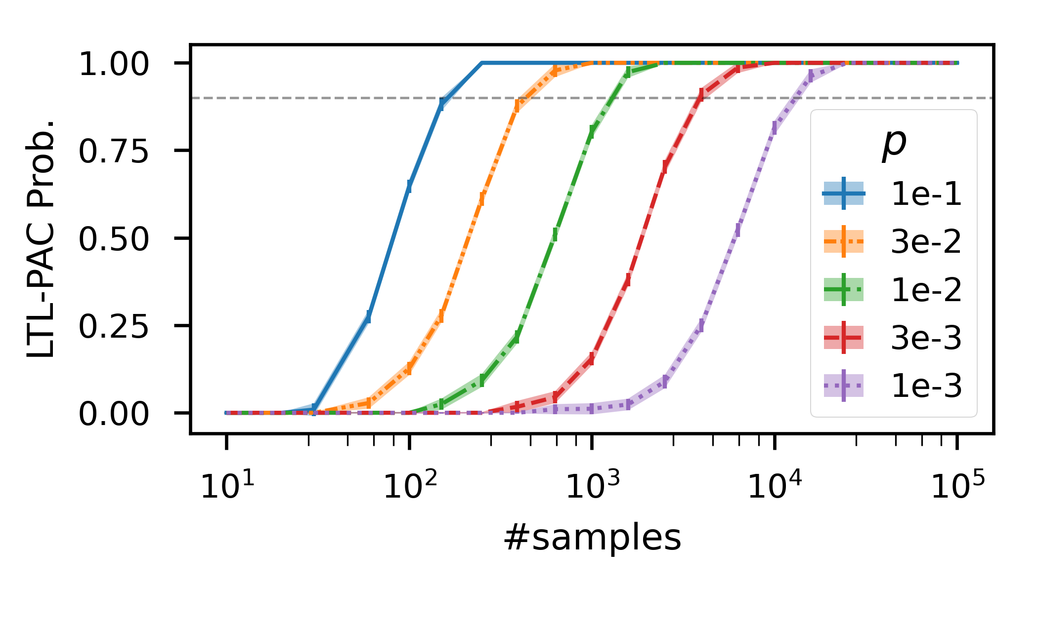
Figure 4: Left: LTL-PAC probabilities vs. number of samples, varying parameters $p$. Right: number of samples needed to reach 0.9 LTL-PAC probability vs. parameter $p$.

5.2 Results

Figure 4 presents the results for the algorithm in Bozkurt et al. (2020) with the setting of Multi-discount, Q-learning, and the first LTL-MDP pair. On the left, we plot the LTL-PAC probabilities vs. the number of samples $N$, one curve for each $p$. On the right, we plot the intersections of the curves in the left plot with a horizontal cutoff of $0.9$.

As we see from the left plot of Figure 4, for each $p$, the curve starts at $0$ and grows to $1$ in a sigmoidal shape as the number of samples increases. However, as $p$ decreases, the MDP becomes harder: As shown on the right plot of Figure 4, the number of samples required to reach the particular LTL-PAC probability of $0.9$ grows exponentially. Results for other algorithms, environments and LTL formulas are similar and lead to the same conclusion.

5.3 Conclusion

Since the transition probabilities ($p$ in this case) are unknown in practice, one can’t know which curve in the left plot a given environment will follow. Therefore, given any finite number of samples, these reinforcement-learning algorithms cannot provide guarantees on the LTL-PAC probability of the learned policy. This result supports Theorem 1.

6 Directions Forward

We have established the intractability of reinforcement learning for infinite-horizon LTL objectives. Specifically, for any infinite-horizon LTL objective, the learned policy need not perform near-optimally given any finite number of environment interactions. This intractability is undesirable in applications that require strong guarantees, such as traffic control, robotics, and autonomous vehicles (Temizer et al., 2010; Kober et al., 2013; Schwarting et al., 2018).

Going forward, we categorize approaches that either focus on tractable objectives or weaken the guarantees required by an LTL-PAC algorithm. We obtain the first category from the reverse direction of Theorem 1, and each of the other categories by relaxing a specific requirement that Theorem 1 places on an algorithm. Further, we classify previous approaches into these categories.

6.1 Use a Finitary Objective

Researchers have introduced specification languages that express finitary properties and have applied reinforcement learning to objectives expressed in these languages (Henriques et al., 2012; Jothimurugan et al., 2019). One value proposition of these approaches is that they provide succinct specifications because finitary properties written in LTL directly are verbose. For example, the finitary property “$a$ holds for $100$ steps” is equivalent to an LTL formula with a conjunction of $100$ terms: $a\land\mathsf{X}a\land\dots\land(\underbrace{\mathsf{X}\dots\mathsf{X}}_{99\text{ times}}a).$

For these succinct specification languages, by the reduction of these languages to finitary properties and the reverse direction of Theorem 1, there exist reinforcement-learning algorithms that give LTL-PAC guarantees.

6.2 Best-effort Guarantee

The definition of LTL-PAC (Definition 3) requires a reinforcement-learning algorithm to learn a policy with satisfaction probability within $\epsilon$ of optimal, for all $\epsilon\,{>}\,0$. However, it is possible to relax this quantification over $\epsilon$ so that an algorithm only returns a policy with the best-available $\epsilon$ it finds.

For example, Ashok et al. (2019) introduced a reinforcement-learning algorithm for objectives in the $\mathit{{Guarantee}}$ class. Using a specified time budget, the algorithm returns a policy and an $\epsilon$. Notably, it is possible for the returned $\epsilon$ to be $1$, a vacuous bound on performance.

6.3 Know More About the Environment

The definition of LTL-PAC (Definition 3) requires a reinforcement-learning algorithm to provide a guarantee for all environments. However, on occasion, one can have prior information on the transition probabilities of the MDP at hand.

For example, Fu and Topcu (2014) introduced a reinforcement-learning algorithm with a PAC-MDP guarantee that depends on the time horizon until the MDP reaches a steady state. Given an MDP, this time horizon is generally unknown; however, if one has knowledge of this time horizon a priori, it constrains the set of MDPs and yields an LTL-PAC guarantee dependent on this time horizon.

As another example, Brázdil et al. (2014) introduced a reinforcement-learning algorithm that provides an LTL-PAC guarantee provided a declaration of the minimum transition probability of the MDP. This constraint, again, bounds the space of considered MDPs.

6.4 Use an LTL-like Objective

Theorem 1 only considers LTL objectives. However, one opportunity for obtaining a PAC guarantee is to change the problem—use a specification language that is LTL-like, defining similar temporal operators but also giving those operators a different, less demanding, semantics.

6.4.1 LTL-in-the-limit Objectives

One line of work (Sadigh et al., 2014; Hahn et al., 2019; Hasanbeig et al., 2019; Bozkurt et al., 2020) uses LTL formulas as the objective, but also introduces one or more hyper-parameters $\boldmath{\lambda}$ to relax the formula’s semantics. The reinforcement-learning algorithms in these works learn a policy for the environment MDP given fixed values of the hyper-parameters. Moreover, as hyper-parameter values approach a limit point, the learned policy becomes optimal for the hyper-parameter-free LTL formula. The relationship between these relaxed semantics and the original LTL semantics is analogous to the relationship between discounted and average-reward infinite-horizon MDPs. Since discounted MDPs are PAC-MDP-learnable (Strehl et al., 2006), we conjecture that these relaxed LTL objectives (at any fixed hyper-parameter setting) are PAC-learnable.

6.4.2 General LTL-like Objectives

Prior approaches (Littman et al., 2017; Li et al., 2017; Giacomo et al., 2019; Camacho et al., 2019) also use general LTL-like specifications that do not or are not known to converge to LTL in a limit. For example, Camacho et al. (2019) introduced the reward-machine objective that uses a finite state automaton to specify a reward function. As another example, Littman et al. (2017) introduced geometric LTL. Geometric LTL attaches a geometrically distributed horizon to each temporal operator. The learnability of these general LTL-like objectives is a potential future research direction.

7 Conclusion

In this work, we have formally proved that infinite-horizon LTL objectives in reinforcement learning cannot be learned in unrestricted environments. By inspecting the core result, we have identified various possible directions forward for future research. Our work resolves the apparent lack of a formal treatment of this fundamental limitation of infinite-horizon objectives, helps increase the community’s awareness of this problem, and will help organize the community’s efforts in reinforcement learning with LTL objectives.

References

- Alur et al. [2021] Rajeev Alur, Suguman Bansal, Osbert Bastani, and Kishor Jothimurugan. A framework for transforming specifications in reinforcement learning. arXiv preprint: 2111.00272, 2021.
- Ashok et al. [2019] Pranav Ashok, Jan Křetínský, and Maximilian Weininger. Pac statistical model checking for markov decision processes and stochastic games. In CAV, 2019.
- Bozkurt et al. [2020] Alper Bozkurt, Yu Wang, Michael Zavlanos, and Miroslav Pajic. Control synthesis from linear temporal logic specifications using model-free reinforcement learning. In ICRA, 2020.
- Brázdil et al. [2014] Tomáš Brázdil, Krishnendu Chatterjee, Martin Chmelík, Vojtěch Forejt, Jan Křetínský, Marta Kwiatkowska, David Parker, and Mateusz Ujma. Verification of markov decision processes using learning algorithms. In ATVA, 2014.
- Camacho et al. [2019] Alberto Camacho, Rodrigo Toro Icarte, Toryn Q. Klassen, Richard Valenzano, and Sheila A. McIlraith. Ltl and beyond: Formal languages for reward function specification in reinforcement learning. In IJCAI, 2019.
- Dann et al. [2019] Christoph Dann, Lihong Li, Wei Wei, and Emma Brunskill. Policy certificates: Towards accountable reinforcement learning. In ICML, 2019.
- Dewey [2014] Dan Dewey. Reinforcement learning and the reward engineering principle. In AAAI Spring Symposia, 2014.
- Fiechter [1994] Claude-Nicolas Fiechter. Efficient reinforcement learning. In COLT, 1994.
- Fu and Topcu [2014] Jie Fu and Ufuk Topcu. Probably approximately correct MDP learning and control with temporal logic constraints. In Robotics: Science and Systems X, 2014.
- Giacomo et al. [2019] Giuseppe De Giacomo, L. Iocchi, Marco Favorito, and F. Patrizi. Foundations for restraining bolts: Reinforcement learning with ltlf/ldlf restraining specifications. In ICAPS, 2019.
- Grill et al. [2016] Jean-Bastien Grill, Michal Valko, and R. Munos. Blazing the trails before beating the path: Sample-efficient monte-carlo planning. In NIPS, 2016.
- Hahn et al. [2019] Ernst Moritz Hahn, Mateo Perez, Sven Schewe, Fabio Somenzi, Ashutosh Trivedi, and Dominik Wojtczak. Omega-regular objectives in model-free reinforcement learning. In TACAS, 2019.
- Hasanbeig et al. [2019] M. Hasanbeig, Yiannis Kantaros, A. Abate, D. Kroening, George Pappas, and I. Lee. Reinforcement learning for temporal logic control synthesis with probabilistic satisfaction guarantees. In CDC, 2019.
- Henriques et al. [2012] David Henriques, João G. Martins, Paolo Zuliani, André Platzer, and Edmund M. Clarke. Statistical model checking for markov decision processes. In QEST, 2012.
- Jiang et al. [2020] Yuqian Jiang, Sudarshanan Bharadwaj, Bo Wu, Rishi Shah, Ufuk Topcu, and Peter Stone. Temporal-logic-based reward shaping for continuing learning tasks. arXiv preprint: 2007.01498, 2020.
- Jothimurugan et al. [2019] Kishor Jothimurugan, R. Alur, and Osbert Bastani. A composable specification language for reinforcement learning tasks. In NeurlPS, 2019.
- Kakade [2003] Sham M. Kakade. On the Sample Complexity of Reinforcement Learning. PhD thesis, Gatsby Computational Neuroscience Unit, UCL, 2003.
- Kearns and Singh [2002] Michael Kearns and Satinder Singh. Near-optimal reinforcement learning in polynomial time. Machine Learning, 49(2), 2002.
- Kearns et al. [1999] Michael Kearns, Yishay Mansour, and Andrew Y. Ng. Approximate planning in large pomdps via reusable trajectories. In NIPS, 1999.
- Kober et al. [2013] Jens Kober, J. Bagnell, and Jan Peters. Reinforcement learning in robotics: A survey. The International Journal of Robotics Research, 32, 2013.
- Li et al. [2017] Xiao Li, C. Vasile, and C. Belta. Reinforcement learning with temporal logic rewards. IROS, 2017.
- Littman et al. [2017] Michael L. Littman, Ufuk Topcu, Jie Fu, Charles Isbell, Min Wen, and James MacGlashan. Environment-independent task specifications via gltl. arXiv preprint: 1704.04341, 2017.
- Manna and Pnueli [1987] Zohar Manna and Amir Pnueli. A hierarchy of temporal properties. In PODC, 1987.
- Pnueli [1977] Amir Pnueli. The temporal logic of programs. In FOCS, 1977.
- Puterman [1994] Martin L. Puterman. Markov Decision Processes—Discrete Stochastic Dynamic Programming. John Wiley & Sons, Inc., 1994.
- Sadigh et al. [2014] Dorsa Sadigh, Eric S. Kim, Samuel Coogan, S. Shankar Sastry, and Sanjit A. Seshia. A learning based approach to control synthesis of markov decision processes for linear temporal logic specifications. In CDC, 2014.
- Schwarting et al. [2018] Wilko Schwarting, Javier Alonso-Mora, and Daniela Rus. Planning and decision-making for autonomous vehicles. Annual Review of Control, Robotics, and Autonomous Systems, 1, 2018.
- Strehl et al. [2006] Alexander Strehl, Lihong Li, Eric Wiewiora, John Langford, and Michael Littman. Pac model-free reinforcement learning. In ICML, 2006.
- Sutton and Barto [1998] Richard S. Sutton and Andrew G. Barto. Reinforcement Learning: An Introduction. The MIT Press, 1998.
- Temizer et al. [2010] Selim Temizer, Mykel Kochenderfer, Leslie Kaelbling, Tomas Lozano-Perez, and James Kuchar. Collision avoidance for unmanned aircraft using markov decision processes. In AIAA GNC, 2010.
- Valiant [1984] L. G. Valiant. A theory of the learnable. Communications of the ACM, 27(11), 1984.