Super-polynomial accuracy of one dimensional randomized nets using the median-of-means

Abstract

Let $f$ be analytic on $[0,1]$ with $|f^{(k)}(1/2)|\leqslant A\alpha^{k}k!$ for some constants $A$ and $\alpha<2$ and all $k\geqslant 1$. We show that the median estimate of $\mu=\int_{0}^{1}f(x)\,\mathrm{d}x$ under random linear scrambling with $n=2^{m}$ points converges at the rate $O(n^{-c\log(n)})$ for any $c<3\log(2)/\pi^{2}\approx 0.21$. We also get a super-polynomial convergence rate for the sample median of $2k-1$ random linearly scrambled estimates, when $k/m$ is bounded away from zero. When $f$ has a $p$’th derivative that satisfies a $\lambda$-Hölder condition then the median-of-means has error $O(n^{-(p+\lambda)+\epsilon})$ for any $\epsilon>0$, if $k\to\infty$ as $m\to\infty$. The proof techniques use methods from analytic combinatorics that have not previously been applied to quasi-Monte Carlo methods, most notably an asymptotic expression from Hardy and Ramanujan on the number of partitions of a natural number.

1 Introduction

In this paper we introduce and study a median-of-means approach to randomized quasi-Monte Carlo (RQMC) sampling. Specifically, for $f:[0,1]\to\mathbb{R}$ we let $\hat{\mu}_{r}$ for $r=1,\dots,2k-1$ be independent estimates of $\mu=\int_{0}^{1}f(x)\,\mathrm{d}x$ computed using the random linear scrambling of Matoušek, (1998) applied to a $(0,m,1)$-net in base $2$ and our estimate of $\mu$ is $\hat{\mu}^{(k)}=\mathrm{med}(\hat{\mu}_{1},\dots,\hat{\mu}_{2k-1})$. We find for some infinitely differentiable integrands, that this median of means approach converges faster than any polynomial rate in $n=2^{m}$. By this we mean that for some $c>0$ the probability of an error larger than $n^{-c\log(n)}$ approaches zero as the number of sampled points $n=2^{m}\to\infty$.

A key ingredient in the proofs is the formula by Hardy and Ramanujan, (1918) for the number $p(n)$ of ways to partition the natural number $n$ into a sum of natural numbers. Their formula for this is

$$p(n)\sim\frac{1}{n4\sqrt{3}}\exp\Bigl{(}\pi\Bigl{(}\frac{2n}{3}\Bigr{)}^{1/2}\Bigr{)}.$$

We believe that this use of analytic combinatorics in RQMC is new and we expect further connections to develop.

There have been several recent results on super-polynomial convergence for quasi-Monte Carlo (QMC). Suzuki, (2017), working in a weighted space of infinitely differentiable functions on $[0,1]^{d}$, proved the existence of digital nets with worst case error $C(d)\exp(-c(d)\log(n)^{2})$. Under further conditions on the weights defining the space, a dimension free worst case error $C\exp(-c\log(n)^{p})$ holds for some $1<p<2$. Dick et al., (2017) give a construction of a super-polynomially convergent method. At a cost of $O(nd\log(n)^{2})$ they use a component-by-component construction to get dimension-independent super-polynomial convergence using interlaced polynomial lattice rules. These are higher order digital nets. A higher order digital net can attain an error of $\tilde{O}(n^{-\alpha})$ when the integrand’s mixed partial derivatives of total order up to the integer $\alpha\geqslant 1$ are all in $L^{2}[0,1]^{d}$ (Dick,, 2011). Here $\tilde{O}$ means that logarithmic factors are not shown. Under scrambling, Dick, (2011) shows that the root mean squared error (RMSE) is $\tilde{O}(n^{-\alpha-1/2})$. To obtain super-polynomial convergence Dick et al., (2017) must let the order of their higher-order digital nets increase with $n$. The median of means formulation allows one to use ordinary scrambled Sobol’ points though in some uses we must take a median of a (slowly) growing number $k$ of replicates. The LatNet builder tool of L’Ecuyer et al., (2022) constructs QMC and RQMC point sets using some random searches. Those searches seek to optimize a figure of merit (FOM) that quantifies worst case error over a class of integrands. For the precise definitions of each FOM, see that paper. Figure 1 there shows some examples where the median FOM shows curvature on a log-log scale for dimension $d=6$. This is consistent with super-polynomial accuracy, though they present a median FOM instead of the FOM of a median estimate.

The algorithm we study here provides another approach. We will see that when $f$ is smooth, most of the randomized net estimates are very close to the true value, for large $m$. The variance is dominated by a relatively small number of bad outcomes. By taking the median of a number of independent estimates we can reduce the impact of the few bad outcomes. Each RQMC estimate is a mean of function evaluations. Then our combined estimates are a median-of-means.

Median-of-means algorithms have many uses in theoretical computer science, though the means used there have not usually been based on RQMC. See for example, Jerrum et al., (1986) and Lecué and Lerasle, (2020). Kunsch et al., (2019) present several uses of the median of means in two stage numerical integration algorithms and they give further references to the literature. Since our preprint appeared, there has been further work on median methods for QMC by Goda and L’Ecuyer, (2022). They choose rank one lattice generating vectors completely at random for integration problems in Korobov spaces and they choose polynomial lattice rules randomly for some weighted Sobolov spaces. By taking the median of a number of such randomly generated estimates they attain the best convergence rates possible for the smoothness levels they study and they are able to avoid complicated parameter searches. Hofstadler and Rudolf, (2022) use median of means to get some strong laws of large numbers for integration methods. Gobet et al., (2022) use median of means to get robust RQMC estimates.

An outline of this paper is as follows. Section 2 provides some notation and definitions of the scrambling we use and the resulting estimates. One key quantity is a scrambling matrix $M$ with $m$ columns and entries in $\{0,1\}$. The accuracy of RQMC is limited by phenomena where for some non-empty $L\subset\mathbb{N}$, the rows of $M$ for $\ell\in L$ sum to $\boldsymbol{0}$ in $\mathbb{F}_{2}^{m}$. Section 3 explains this bottleneck to convergence and Theorem 3.1 there writes the RQMC error as a sum of random variables, one for each problematic subset $L$. This section is less technical than the later ones with our proofs. Section 4 has a one dimensional numerical example. We see superlinear convergence for the median of $11$ RQMC replicates, up to a point. The RMSE reaches an asymptote for a Sobol’ sequence computed to $32$ bits. Switching to a $64$ bit computation, the superlinearity continues to some higher sample sizes. There is also a six dimensional example, where the standard deviation of median estimates drops faster than that of mean estimates. Section 5 studies the population median of scrambled nets for dimension $d=1$. This is the median of the distribution of the RQMC estimate. Theorem 5.6 establishes a super-polynomial rate for that quantity for certain infinitely differentiable functions. A critical step there is to bound the number of nonempty subsets $L\subset\mathbb{N}$ that have a small value of $\sum_{\ell\in L}\ell$. We do this using combinatorial results including the one by Hardy and Ramanujan, (1918). The comprehensive reference is Flajolet and Sedgewick, (2009). Theorem 5.10 provides super-polynomial convergence for the median of $2k-1$ independently generated RQMC estimates. Section 6 considers the case where the $p$’th derivative of $f$ satisfies a $\lambda$-Hölder condition for $0<\lambda\leqslant 1$. Theorem 6.1 there bounds the probability that the error is much more than $n^{-p-\lambda}$ with corollaries showing super-polynomial convergence for the population median and the median of $2k-1$ independent estimates.

We close this section with a few contextual remarks. In the one dimensional setting, there are already very accurate integration rules for extremely smooth integrands (Davis and Rabinowitz,, 1984). The RQMC method here has an advantage in being an equally weighted average of the $n$ function values, instead of having large weights of both positive and negative signs. The one dimensional case will take on greater interest if the findings and proofs in this article can be generalized to $d\geqslant 1$. The multidimensional example in Section 4 is therefore encouraging as are the empirical results in L’Ecuyer et al., (2022).

One of the original motivations for RQMC was to get error estimates. It later emerged that randomizing QMC can also increase accuracy (Owen,, 1997). Error estimation for a median of independently sampled means is more complicated than for a mean of such means. We can readily get a nonparametric confidence interval for the population median of the $\hat{\mu}_{r}$, using the binomial distribution because the true median $\theta$ satisfies $\Pr(\hat{\mu}_{r}<\theta)=1/2$. However, the quantity of most direct interest is $\mathbb{E}(\hat{\mu}_{r})$ not $\mathrm{med}(\hat{\mu}_{r})$.

We had initially considered the case where instead of a random linear scramble we had taken a completely random generator matrix with all entries independent and identically (IID) $\mathbb{U}\{0,1\}$ random variables. A similar result holds: the median estimate converges with super-polynomial accuracy for certain infinitely differentiable $f$, though of course the bad outcomes can be even worse. For instance, there is a $2^{-m^{2}}$ probability that the upper $m\times m$ submatrix of the generator matrix is all zeros. Then all $n=2^{m}$ RQMC points would lie in the interval $[0,1/n]$ and the resulting error would generally fail to vanish as $n\to\infty$.

2 Notation and background

We study the random linear scrambling of Matoušek, (1998) including a digital shift, in one dimension. Our focus is on base $2$ apart from a few remarks later. For an integrand $f:[0,1]\to\mathbb{R}$ we will estimate $\mu=\int_{0}^{1}f(x)\,\mathrm{d}x$ assumed to exist by $\hat{\mu}=(1/n)\sum_{i=0}^{n-1}f(x_{i})$ for carefully chosen points $x_{i}\in[0,1]$.

We use $\mathbb{N}$ for the set of positive integers. For $m\in\mathbb{N}$, we let $[m]$ denote the set $\{1,\ldots,m\}$ and for $n\in\mathbb{N}$ we let $\mathbb{Z}_{n}$ denote the set $\{0,1,\dots,n-1\}$. We investigate a scrambled digital net of $n=2^{m}$ points $x_{i}\in[0,1)$ for $i=0,1,\dots,n-1$.

We will make frequent use of sets $L\subset\mathbb{N}$ of finite cardinality. We write $|L|$ for their cardinality as well as $\|L\|_{1}=\sum_{\ell\in L}\ell$ and some additional notation about these sets $L$ will be introduced as needed. For a matrix $M$ we use $M(L,:)$ to denote the submatrix whose row indices are in $L$ and to extract a single row we write $M(\ell,:)$ instead of $M(\{\ell\},:)$.

The indicator function of the event $E$ is sometimes written $\boldsymbol{1}\{E\}$. This quantity takes the value $1$ when $E$ holds and $0$ otherwise.

We assume throughout that $C\in\{0,1\}^{m\times m}$ is a nonrandom matrix that is of full rank $m$ over $\mathbb{F}_{2}$, that is, it has full rank in arithmetic modulo 2. This matrix $C$ defines the ‘unscrambled’ version of our QMC points which will be a $(0,m,1)$-net in base $2$. For instance $C$ could be the $m\times m$ identity matrix as it would be for the van der Corput points.

For $i\in\mathbb{Z}_{2^{m}}$ we let $\vec{i}=(i_{1},i_{2},\dots,i_{m})^{\mathsf{T}}$ where $i=i_{1}+2i_{2}+4i_{3}+\cdots+2^{m-1}i_{m}$. For $a=\sum_{k=1}^{m}a_{k}2^{-k}\in[0,1)$ we let $\vec{a}=(a_{1},a_{2},\dots,a_{m})^{\mathsf{T}}$. These two definitions intersect only for $\{0\}$ where they both yield $\boldsymbol{0}$. The representation for $a\in[0,1)$ can be taken to any finite number $E\geqslant m$ of bits, that we denote by $\vec{a}[E]$ when we need to specify the precision. When $a$ has two base $2$ representations, we work with the one that has finitely many nonzero bits. The points of the unscrambled net are given by $a_{i}\in\{k/2^{m}\mid k\in\mathbb{Z}_{2^{m}}\}\subset[0,1)$ that satisfy

$$\vec{a}_{i}=C\vec{i}\quad\text{for $i\in\mathbb{Z}_{2^{m}}$}$$

so that

$$a_{i}=\sum_{k=1}^{m}2^{-k}a_{ik}\quad\text{for bits}\quad a_{ik}=\sum_{j=1}^{k}C_{kj}i_{j}\ \mathsf{mod}\ 2.$$

In our presentation below we will omit noting that bitwise arithmetic is done modulo two, when that is clear from context.

To scramble the points, we introduce a random matrix $M\in\{0,1\}^{E\times m}$ for $E\geqslant m$. The upper triangular elements of $M$ are all $0$, the diagonal elements of $M$ are all $1$, and the elements below the diagonal are IID $\mathbb{U}\{0,1\}$.

We also introduce a random digital shift $D=\sum_{k=1}^{\infty}2^{-k}D_{k}$ with bits ${D}_{k}$ that are independent $\mathbb{U}\{0,1\}$ variables independent of $M$. Note that $\Pr(0\leqslant D<1)=1$. The random digital shift serves to make the estimates $\hat{\mu}$ unbiased estimates of $\mu$ and our proofs require that property.

For $i\in\mathbb{Z}_{2^{m}}$, linearly scrambled points $x_{i}$ to precision $E$ without a digital shift are defined by

$$\vec{x}_{i}=\vec{x}_{i}[E]=M\vec{a}_{i}=MC\vec{i}$$ (2.1)

for bits

$$a_{ik}=\sum_{j=1}^{k}C_{kj}i_{j}\quad\text{and}\quad x_{ik}=\sum_{j=1}^{k}M_{kj}a_{ij}.$$

When we add the random digital shift, we randomize infinitely many bits. We define scrambling of precision $E$ to mean that $x_{i}$ has bits

$$x_{ik}=x_{ik}[E]=\begin{cases}\sum_{j=1}^{k}M_{kj}a_{ij}+D_{k},&k\leqslant E\\ D_{k},&k>E.\end{cases}$$ (2.2)

We will use the term ‘random linear scrambling’ to refer to linear scrambling that includes the digital shift. This usage is common. Another usage calls that affine scrambling with linear scrambling excluding the digital shift.

Let $f:[0,1]\to\mathbb{R}$. We need to specify the precision of our estimates and to do this, we define

$$\hat{\mu}_{E}=\hat{\mu}_{E}(f)=\frac{1}{n}\sum_{i=0}^{n-1}f(x_{i})$$

where the bits of $x_{i}$ are given by (2.2). When $f$ is continuous on $[0,1]$, define

$$\hat{\mu}_{\infty}=\lim_{E\to\infty}\hat{\mu}_{E}.$$

Later when we replicate these quantities, the replicates will be denoted $\hat{\mu}_{E,r}$ and $\hat{\mu}_{\infty,r}$. We let $\omega_{f}(t)$ denote the modulus of continuity of $f$ over $[0,1]$. Later, $\omega_{f}(1)$ will be a convenient shorthand for $\sup_{0\leqslant x\leqslant 1}f(x)-\inf_{0\leqslant x\leqslant 1}f(x)$.

Lemma 2.1.

For any $M\in\{0,1\}^{\infty\times m}$ and $D\in[0,1)$

$$|\hat{\mu}_{\infty}-\hat{\mu}_{E}|\leqslant\omega_{f}\Bigl{(}\frac{1}{2^{E}}\Bigr{)}$$

where $\hat{\mu}_{E}$ is constructed using the first $E\geqslant m$ rows of $M$.

Proof.

Let $x_{i}[E]$ be $x_{i}$ under scrambling with precision $E$ and $x_{i}[\infty]$ be $x_{i}$ under scrambling in the infinite precision limit. For any given $M$ and $D$ in random linear scrambling, $x_{i}[E]$ has the same first $E$ bits as $x_{i}[\infty]$, so

$$\bigl{|}x_{i}[E]-x_{i}[\infty]\bigr{|}\leqslant\sum_{k=E+1}^{\infty}\frac{1}{2^{k}}|x_{ik}[E]-x_{ik}[\infty]|\leqslant\frac{1}{2^{E}},$$

where $k$ indexes the bits of $x_{i}[E]$ and $x_{i}[\infty]$. Hence

$$|\mu_{\infty}-\mu_{E}|\leqslant\frac{1}{n}\sum_{i=0}^{n-1}|f(x_{i}[E])-f(x_{i}[\infty])|\leqslant\omega_{f}\Bigl{(}\frac{1}{2^{E}}\Bigr{)}.\qed$$

The main object of our study is the median of $2k-1$ independently sampled replicates of a randomized QMC algorithm on $m$ points. We may take $k$ to be a function of $m$. We write $k=\Omega(m)$ to mean that $\lim\inf_{m\to\infty}k(m)/m>0$ and similarly $k=\Omega(m^{2})$ means that $\liminf_{m\to\infty}k(m)/m^{2}>0$. In practice $k$ would be non-decreasing in $m$ though our results do not require this.

3 A bottleneck in convergence

It is well known that the variance of $\hat{\mu}$ under nested uniform scrambling attains $O(n^{-3})$ convergence when $d=1$ and $f^{\prime}\in C[0,1]$, a great improvement upon the $O(n^{-1})$ rate of naive Monte Carlo. Corollary 3.8 of Wiart et al., (2021) shows that random linear scrambling with a digital shift has the same variance as nested uniform scrambling for $(0,m,1)$-nets. Increased smoothness does not improve this rate outside of trivial settings with zero variance. Here we give a simple argument to illustrate that limitation. Understanding such bounds leads us to an expression for the integration error below, on which we base our study of medians.

If $n=2^{m}$ and $M(m+1,:)$ happens to be $\boldsymbol{0}$, then by the relationship $x_{i,m+1}=\sum_{j=1}^{m+1}M_{m+1,j}a_{ij}+D_{m+1}$, we immediately see that $x_{i,m+1}=D_{m+1}$ for all $i$. Geometrically, this means for each interval $[i/n,(i+1)/n)$, the samples are either all in the left half interval (if $D_{m+1}=0$) or all in the right half interval (if $D_{m+1}=1$). If we assume for simplicity that $D_{m+1}=1$ and the scrambling has precision $m+1$, then each sample is actually uniform on the right half of the interval it lands in and we can approximate the error by its expectation given that $M(m+1,:)=\boldsymbol{0}$ and $D_{m+1}=1$ as:

$$\hat{\mu}_{m+1}-\mu \approx\sum_{i=0}^{n-1}\biggl{(}2\int_{\frac{i+0.5}{n}}^{\frac{i+1}{n}}f(x)\,\mathrm{d}x-\int_{\frac{i}{n}}^{\frac{i+1}{n}}f(x)\,\mathrm{d}x\biggr{)}$$

$$\approx\sum_{i=0}^{n-1}\int_{\frac{i+0.5}{n}}^{\frac{i+1}{n}}f\Bigl{(}\frac{i+0.5}{n}\Bigr{)}+f^{\prime}\Bigl{(}\frac{i+0.5}{n}\Bigr{)}\Bigl{(}x-\frac{i+0.5}{n}\Bigr{)}\,\mathrm{d}x$$

$$\phantom{=}-\sum_{i=0}^{n-1}\int_{\frac{i}{n}}^{\frac{i+0.5}{n}}f\Bigl{(}\frac{i+0.5}{n}\Bigr{)}+f^{\prime}\Bigl{(}\frac{i+0.5}{n}\Bigr{)}\Bigl{(}x-\frac{i+0.5}{n}\Bigr{)}\,\mathrm{d}x$$

$$=\frac{1}{8n^{2}}\sum_{i=0}^{n-1}f^{\prime}\Bigl{(}\frac{i+0.5}{n}\Bigr{)}.$$

If instead $D_{m+1}=0$, then all the $x_{i}$ fall in the left half interval and the expected error is like that above, but with the opposite sign. Hence the conditional expectation of $|\hat{\mu}_{\mathrm{RQMC}}-\mu|$ cannot be of lower order than $n^{-1}$ when $M(m+1,:)=\boldsymbol{0}$. Because each entry of $M(m+1,:)$ is independently 0 or 1 with equal probability, $\Pr(M(m+1,:)=\boldsymbol{0})=2^{-m}$ and those rare outcomes alone make $\mathrm{Var}(\hat{\mu}_{\mathrm{RQMC}})$ at least of order $2^{-m}(n^{-1})^{2}=n^{-3}$. Theorem 3.1 below makes the above reasoning rigorous.

The main takeaway is that the rare event $M(m+1,:)=\boldsymbol{0}$ makes a major contribution to the variance. Curious readers may ask what happens if we explicitly avoid the event $M(m+1,:)=\boldsymbol{0}$. This is indeed what is done in the affine striped matrix (ASM) scrambling from Owen, (2003). For base 2, the matrix $M$ of ASM scrambling is nonrandom and described by $M_{kj}=1$ for $k\geqslant j$ and $M_{kj}=0$ for $k<j$. Therefore $M(m+1,:)=\boldsymbol{1}$ and ASM scrambling is able to attain the $\mathrm{Var}(\hat{\mu})=O(n^{-4})$ convergence rate when $f^{\prime\prime}$ is bounded on $[0,1)$ (Owen,, 2003, Proposition 3.7).

A similar question arises: can ASM scrambling converge faster than $O(n^{-4})$ under stronger smoothness assumptions? The answer is again no. Assume for simplicity that $D_{m+1}=D_{m+2}=0$ and that the scrambling has precision $E=m+2$. Because $M(m+1,:)=M(m+2,:)$,

$$x_{i,m+1}=\sum_{j=1}^{m+1}M_{m+1,j}a_{ij}=\sum_{j=1}^{m+1}M_{m+2,j}a_{ij}=x_{i,m+2}.$$

Now within each interval $[i/n,(i+1)/n)$, the sampling is either uniform in the leftmost quarter $[i/n,(i+0.25)/n)$ or uniform in the rightmost quarter $[(i+0.75)/n,(i+1)/n)$. Suppose without loss of generality that the sampling for interval $i$ is in the rightmost quarter. Then as in the analysis of random linear scrambling, we can approximate the integration error over $[i/n,(i+1)/n)$ by

$$4\int_{\frac{i+0.75}{n}}^{\frac{i+1}{n}}f(x)\,\mathrm{d}x-\int_{\frac{i}{n}}^{\frac{i+1}{n}}f(x)\,\mathrm{d}x$$

$$\approx 4\int_{\frac{i+0.75}{n}}^{\frac{i+1}{n}}f\Bigl{(}\frac{i+0.5}{n}\Bigr{)}+f^{\prime}\Bigl{(}\frac{i+0.5}{n}\Bigr{)}\Bigl{(}x-\frac{i+0.5}{n}\Bigr{)}+\frac{1}{2}f^{\prime\prime}\Bigl{(}\frac{i+0.5}{n}\Bigr{)}\Bigl{(}x-\frac{i+0.5}{n}\Bigr{)}^{2}\,\mathrm{d}x$$

$$\phantom{=}-\int_{\frac{i}{n}}^{\frac{i+1}{n}}f\Bigl{(}\frac{i+0.5}{n}\Bigr{)}+f^{\prime}\Bigl{(}\frac{i+0.5}{n}\Bigr{)}\Bigl{(}x-\frac{i+0.5}{n}\Bigr{)}+\frac{1}{2}f^{\prime\prime}\Bigl{(}\frac{i+0.5}{n}\Bigr{)}\Bigl{(}x-\frac{i+0.5}{n}\Bigr{)}^{2}\,\mathrm{d}x$$

$$=\frac{3}{8n^{2}}f^{\prime}\Bigl{(}\frac{i+0.5}{n}\Bigr{)}+\frac{1}{32n^{3}}f^{\prime\prime}\Bigl{(}\frac{i+0.5}{n}\Bigr{)}.$$

When sampling for observation $i$ is in the leftmost quarter the approximate error as above is

$$-\frac{3}{8n^{2}}f^{\prime}\Bigl{(}\frac{i+0.5}{n}\Bigr{)}+\frac{1}{32n^{3}}f^{\prime\prime}\Bigl{(}\frac{i+0.5}{n}\Bigr{)}.$$

The $f^{\prime}$ terms each contribute an error of $O(n^{-2})$. The sign of the $f^{\prime}$ terms depends on the nonrandom $a_{i}$. Carefully chosen $a_{i}$ could possibly bring cancellation among the $f^{\prime}$ terms, leaving a total error $o(n^{-2})$ from the $f^{\prime}$ terms. However, no such cancellation is possible for the $f^{\prime\prime}$ terms. Therefore, if we did manage to cancel the $f^{\prime}$ terms we would still have an error

$$\hat{\mu}_{m+2}-\mu \approx\frac{1}{32n^{3}}\sum_{i=0}^{n-1}f^{\prime\prime}\Bigl{(}\frac{i+0.5}{n}\Bigr{)}.$$

This implies that $|\hat{\mu}_{\mathrm{RQMC}}-\mu|$ is at least of order $n^{-2}$, and so $\mathrm{Var}(\hat{\mu}_{\mathrm{RQMC}})$ cannot converge faster than $O(n^{-4})$. Notice that in this case $M$ is nonrandom, so we do not need to multiply that squared error by an event probability like $2^{-m}$ as we did in the previous example.

One may summarize from the above heuristic reasoning that whenever a set $L$ of rows of $M$ satisfies $\sum_{\ell\in L}M(\ell,:)=\boldsymbol{0}$, there is an associated error of order $2^{-\sum_{\ell\in L}\ell}$. This is indeed true by Theorem 3.1 below. Before stating that theorem we introduce some notation. Let

$$\mathcal{L}=\{L\subset\mathbb{N}\mid 0<|L|<\infty\}.$$

Each $L\in\mathcal{L}$ identifies a set of row indices for $M$. Each of these finite non-empty subsets of natural numbers potentially contributes an error that scales like $2^{-\|L\|_{1}}$ where $\|L\|_{1}=\sum_{\ell\in L}\ell$. We also use $\|D(L)\|_{1}=\sum_{\ell\in L}D_{\ell}$. This quantity will appear as the exponent of $-1$ where only its value modulo two matters.

Theorem 3.1.

Let $f$ be analytic on $[0,1]$ with $|f^{(k)}(1/2)|\leqslant A\alpha^{k}k!$ for some constant $A$, some $\alpha<2$ and all $k\in\mathbb{N}$. If $C\in\{0,1\}^{m\times m}$ is nonsingular, then

$$\hat{\mu}_{\infty}-\mu =\sum_{L\in\mathcal{L}}\boldsymbol{1}\Bigl{\{}\sum_{\ell\in L}M(\ell,:)=\boldsymbol{0}\Bigr{\}}\,S_{L}(D)\,2^{-\|L\|_{1}}B_{L}$$ (3.1)

where

$$S_{L}(D) =\prod_{\ell\in L}(-1)^{D_{\ell}}$$ (3.2)

and scalars $$B_{L}$$ from Appendix A satisfy

$$|B_{L}| \leqslant 6A\bigl{(}|L|\bigr{)}!\Bigl{(}\frac{\alpha/2}{1-\alpha/2}\Bigr{)}^{|L|}.$$ (3.3)

Proof.

See Appendix A. ∎

Remark 3.2.

Notice that $|f^{(k)}(1/2)|\leqslant A\alpha^{k}k!$ for all $k\in\mathbb{N}$ is not really a more stringent assumption than $f$ being analytic on $[0,1]$. To be analytic on a closed interval requires $f$ to be analytic on some open interval containing it. Then for the Taylor expansion of $f$ centered at $1/2$ to have a radius of convergence larger than $1/2$, it is necessary that $|f^{(k)}(1/2)|\leqslant A\alpha^{k}k!$ for some constant $A$ and $\alpha<2$.

We see that for each $L\in\mathcal{L}$, the corresponding term in (3.1) contains a factor depending on $M$ times a factor depending on $D$. It helps that $M$ and $D$ are independent random quantities.

4 Numerical examples

The function $f(x)=x\exp(x)$ has integral $\mu=1$ over $[0,1]$. We selected this $f$ because it is infinitely differentiable as our theory requires, and it is not a polynomial and is not symmetric or antisymmetric. Those are factors that might make a function artificially easy to integrate by a specially tuned numerical method. There is also no special feature in the function at values like $1/2$ or more generally integers divided by a power of $2$ that might confer an advantage for Sobol’ points which are generated in base $2$.

We sampled this function with random linear scrambling for $0\leqslant m\leqslant 15$. For this we used the Sobol function in the QMCPy software of Choi et al., (2021). We took the median of $k=11$ RQMC integral estimates $R=250$ times.

Figure 1 shows how the RMSE of the median of $11$ RQMC estimates decreases with $n$ as open circles connected by dashed lines. It appears to decrease at a superpolynomial rate until it reaches a limit of about $10^{-9}$. The Sobol’ points in QMCPy default to $32$ bits for the linear scramble with the digital shift carried out more bits. Our theory is for infinitely many bits. We redid the computations using $64$ bits for the linear scramble, resulting in the solid points connected by solid lines. With $64$ bits the apparent super-polynomial convergence holds through the entire range of sample sizes in the figure.

The figure also shows the RMSE of a single RQMC estimate of which there were $250\times 11=2750$. There is a reference curve at the $n^{-3/2}$ rate interpolating the value for $n=1$. A dashed line below that by a factor of $\sqrt{11}$ corresponds to accuracy using an average of $11$ RQMC estimates that could have been done at the same cost as the median of $11$ RQMC estimates. In the next sections we prove that the median RQMC estimate converges at a superpolynomial rate. We also show that the sample median of $k$ RQMC estimates attains such a rate when $k$ grows slowly with $m$.

At tiny sample sizes like $1$, $2$ and $4$ we see that a mean of $11$ RQMC estimates was more accurate than a median of $11$ RQMC estimates. By $n\geqslant 16$, we see the median doing better than the dotted reference line applicable to the mean of $11$ RQMC estimates.

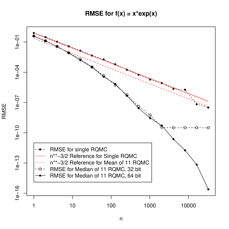
Figure 1: The dashed line with open points shows the RMSE of 250 integral estimates, each of which is the median of 11 RQMC estimates. Those computations were done with $M=32$-bit Sobol’ points. The solid line with solid points repeats that calculation using 64 bits instead of 32. The dashed line with solid points connects RMSEs of 2750 RQMC estimates without taking a median. The solid reference line is proportional to $n^{-3/2}$, running through the plain RQMC value for $n=1$. The dashed line is lower by a factor of $\sqrt{11}$ to estimate the RMSE that a mean of $11$ estimates would have.

We also investigated a six dimensional function that computes a midpoint voltage for an output transformerless (OTL) push-pull circuit. The function is given at Surjanovic and Bingham, (2013) which includes a link to describe the electronics background as well as some code. The results are shown in Figure 2. We used scrambled Sobol’ points from QMCPy. Because the true mean is not known, we plot the standard deviation instead of the RMSE. While the curve shows an apparent better rate in this multivariate problem it does not account for the bias induced by taking a median instead of a mean. That issue is outside the scope of the present article.

We note in passing that graphical rendering applications of QMC while not having much smoothness can also benefit from using a large number $E$ of bits. See Keller, (2013) for a discussion of QMC for rendering.

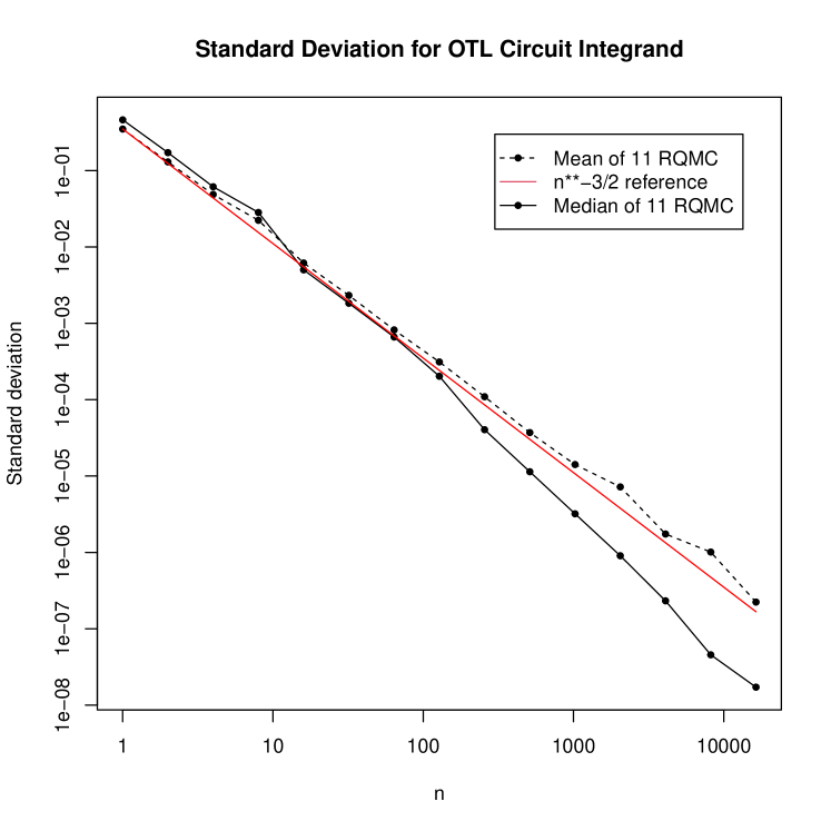
Figure 2: The solid line with solid points shows the standard deviation among 100 replicates that each take the median of 11 independent RQMC estimates. The dashed line with solid points has the standard deviation of 1100 replicates divided by $\sqrt{11}$ to reflect the accuracy of a mean of 11 RQMC estimates. The solid reference line is proportional to $n^{-3/2}$ and passes through the point for $n=1$ and the mean of 11 RQMC estimates.

5 Convergence rate of the median

As we see in Theorem 3.1, sets $L$ with $\sum_{\ell\in L}M(\ell,:)=\boldsymbol{0}$ contribute to the RQMC error and the upper bound on that contribution contains the factor $2^{-\|L\|_{1}}$, so that sets $L$ with small $\|L\|_{1}$ are of great concern. In the examples in Section 3 we saw that this can be the major source of error in both scrambled nets and ASM sampling. Is there a way to avoid such bad events? One approach is to redesign the scrambling to avoid $\sum_{\ell\in L}M(\ell,:)=\boldsymbol{0}$ for certain $L$. See for instance the higher order digital nets of Dick, (2011) and polynomial lattice rules in Goda and Dick, (2015). Another approach, which is the main focus of this paper, is to take the median instead of the mean of several QMC simulations. Below we show that the median of random linear scrambling with infinite precision converges to $\mu$ at a super-polynomial rate when $f$ satisfies the condition in Theorem 3.1.

In random linear scrambling, because $M([m],:)$ is nonsingular and $M(\ell,:)$ for $\ell>m$ has each entry independently $\mathbb{U}\{0,1\}$,

$$\Pr\biggl{(}\,\sum_{\ell\in L}M(\ell,:)=\boldsymbol{0}\biggr{)}=\begin{cases}0,&L\subseteq[m]\\ 2^{-m},&L\nsubseteq[m].\end{cases}$$ (5.1)

As a result, the event $\sum_{\ell\in L}M(\ell,:)=\boldsymbol{0}$ is unlikely to happen for a set $L$ with small $\|L\|_{1}$. We use the next lemma to control the number of $L\in\mathcal{L}$ with small $\|L\|_{1}$.

Lemma 5.1.

Let $\lambda=3(\log(2))^{2}/\pi^{2}\approx 0.146$. Then

$$\lim_{m\to\infty}\sqrt{m}{2^{-m}}\bigl{|}\{L\in\mathcal{L}\mid\|L\|_{1}\leqslant\lambda m^{2}\}\bigr{|}=\frac{3^{1/4}}{2\pi\lambda^{1/4}}.$$ (5.2)

Moreover, for $1\leqslant m\leqslant 512$,

$$\bigl{|}\{L\in\mathcal{L}\mid\|L\|_{1}\leqslant\lambda m^{2}\}\bigr{|}<\frac{0.4\times 2^{m}}{\sqrt{m}}.$$ (5.3)

Proof.

See Appendix B. ∎

The limit in (5.2) holds with $m\to\infty$ through real values. Our primary use of it is for integers $m\geqslant 1$ but we will also use it for non-integers.

Remark 5.2.

The sequence in equation (5.2) is in fact monotonically decreasing for $20\leqslant m\leqslant 512$, so one can reasonably guess that the bound in equation (5.3) applies to $m>512$ as well, although we do not have a proof for this.

Lemma 5.3.

In random linear scrambling, there exists a constant $\overline{C}$ such that for all $m\geqslant 1$ and any $0\leqslant\epsilon<1$,

$$\Pr\biggl{(}\min\Bigl{\{}\|L\|_{1}\bigm{|}L\in\mathcal{L},\sum_{\ell\in L}M(\ell,:)=\boldsymbol{0}\Bigr{\}}\leqslant\lambda(1-\epsilon)m^{2}\biggr{)}<\frac{\overline{C}}{(1-\epsilon)^{{1}/{4}}\sqrt{m}}2^{-{\epsilon m}/{2}}.$$

When $m\leqslant 512$, we can choose $\overline{C}$ to be $0.4$.

Proof.

Equation (5.2) implies that there exists a constant $\overline{C}$ such that $\sqrt{m}2^{-m}\bigl{|}\{L\in\mathcal{L}\mid\|L\|_{1}\leqslant\lambda m^{2}\}\bigr{|}\leqslant\overline{C}$ for all $m\geqslant 1$. We apply this inequality with $m$ replaced by $m\sqrt{1-\epsilon}$ and apply the union bound to all events $\sum_{\ell\in L}M(\ell,:)=\boldsymbol{0}$ with $\|L\|_{1}\leqslant\lambda(1-\epsilon)m^{2}$. We then get

$$\phantom{=}\,\Pr\bigl{(}\,\exists L\in\mathcal{L},\|L\|_{1}\leqslant\lambda(1-\epsilon)m^{2},\sum_{\ell\in L}M(\ell,:)=\boldsymbol{0}\bigr{)}$$

$$\leqslant\sum_{\{L\in\mathcal{L}\,\mid\,\|L\|_{1}\leqslant\lambda(1-\epsilon)m^{2}\}}\Pr\biggl{(}\,\sum_{\ell\in L}M(\ell,:)=\boldsymbol{0}\biggr{)}$$

$$\overset{\mathrm{(i)}}{<}\frac{\overline{C}2^{m\sqrt{1-\epsilon}}}{(1-\epsilon)^{1/4}\sqrt{m}}2^{-m}\overset{\mathrm{(ii)}}{\leqslant}\frac{\overline{C}}{(1-\epsilon)^{1/4}\sqrt{m}}2^{-{\epsilon m}/{2}},$$

where (i) follows from equation (5.1) and (ii) follows from $1-\sqrt{1-\epsilon}\geqslant\epsilon/2$. When $m\leqslant 512$, equation (5.3) shows we can choose $\overline{C}=0.4$. ∎

Remark 5.4.

We will mostly use the above lemma for $\epsilon=0$, in which case

$$\Pr\Bigl{(}\min\bigl{\{}\|L\|_{1}\bigm{|}L\in\mathcal{L},\sum_{\ell\in L}M(\ell,:)=\boldsymbol{0}\bigr{\}}\leqslant\lambda m^{2}\Bigr{)}<\frac{0.4}{\sqrt{m}}$$

when $1\leqslant m\leqslant 512$ and is $O(m^{-1/2})$ as $m\to\infty$.

We are going to apply Chebyshev’s inequality to bound the probability that $\hat{\mu}_{\infty}$ is far from $\mu$. For that, we first prove that the random sign terms $S_{L}(D)=(-1)^{\|D(L)\|_{1}}$ in Theorem 3.1 are pairwise independent Rademacher (i.e., $\mathbb{U}\{-1,1\}$) random variables.

Lemma 5.5.

For $L\in\mathcal{L}$, let $S_{L}(D)$ be as in equation (3.2). Then for $L,L^{\prime}\in\mathcal{L}$ $\Pr(S_{L}(D)=1)=\Pr(S_{L}(D)=-1)=1/2$ and for $L\neq L^{\prime}$

$$\Pr(S_{L}(D)=1,S_{L^{\prime}}(D)=1)=\frac{1}{4}.$$

Proof.

The entries of $D$ are $D_{\ell}\stackrel{{\scriptstyle\mathrm{iid}}}{{\sim}}\mathbb{U}\{0,1\}$, so $(-1)^{D_{\ell}}\stackrel{{\scriptstyle\mathrm{iid}}}{{\sim}}\mathbb{U}\{-1,1\}$ and then

$$\mathbb{E}(S_{L}(D))=\prod_{\ell\in L}\mathbb{E}((-1)^{D_{\ell}})=0.$$

This combined with $S_{L}(D)\in\{-1,1\}$ implies that $\Pr(S_{L}(D)=1)=1/2$. If $L\neq L^{\prime}$, then letting $\triangle$ denote the symmetric difference of sets,

$$\mathbb{E}\bigl{(}S_{L}(D)S_{L^{\prime}}(D)\bigr{)} =\prod_{\ell\in L\triangle L^{\prime}}\mathbb{E}\bigl{(}(-1)^{D_{\ell}}\bigr{)}=0.$$ (5.4)

Now let $\Pr(S_{L}(D)=1,S_{L^{\prime}}(D)=1)=1/4+\delta$. From the symmetry of Rademacher random variables, we get $\Pr(S_{L}(D)=1,S_{L^{\prime}}(D)=-1)=1/4-\delta$ and $\Pr(S_{L}(D)=-1,S_{L^{\prime}}(D)=1)=1/4-\delta$. Then by subtraction we have $\Pr(S_{L}(D)=-1,S_{L^{\prime}}(D)=-1)=1/4+\delta$. From (5.4) we get $\delta=0$ so $\Pr(S_{L}(D)=1,S_{L^{\prime}}(D)=1)=1/4$ meaning that $S_{L}(D)$ and $S_{L^{\prime}}(D)$ are independent. ∎

Now we are ready to prove the main theorem concerning the super-polynomial convergence rate of the median of random linear scrambling. Then we will have one corollary for $m\leqslant 512$ and another for $m\to\infty$.

Theorem 5.6.

Let the integrand $f$ satisfy the conditions of Theorem 3.1 with constants $A$ and $\alpha$ given there. Let $\lambda$ be as in Lemma 5.1 and set $\theta={\alpha}/(e(2-\alpha))$. Then for any $\eta>0$ and $m\geqslant 3$, the random linear scrambling estimate $\hat{\mu}_{\infty}$ satisfies

$$\Pr\Big{(}|\hat{\mu}_{\infty}-\mu|>\frac{A}{\sqrt{\eta}}2^{-\lambda m^{2}}\sqrt{C_{\theta}(\theta\sqrt{2\lambda}m)^{2\sqrt{2\lambda}m}+64}\Big{)}<\eta+\frac{\overline{C}}{\sqrt{m}}$$ (5.5)

where $C_{\theta}$ is a positive number depending only on $\theta$, defined in equation (5.12) and $\overline{C}$ is the constant from Lemma 5.3. If $m\leqslant 512$, we can replace $\overline{C}$ by $0.4$. If also $m\geqslant\max((\sqrt{2\lambda}\theta)^{-1},3\log(\theta m)+3)$, then we can replace $C_{\theta}$ by $3770\max(1,\theta^{-1})$.

Proof.

First we condition on $M$ and apply Chebyshev’s inequality. For $c>0$

$$\Pr\bigl{(}|\hat{\mu}_{\infty}-\mu|>c\!\mid\!M\bigr{)} \leqslant\frac{\mathrm{Var}(\hat{\mu}_{\infty}-\mu\!\mid\!M)}{c^{2}}.$$

By Theorem 3.1 and Lemma 5.5,

$$\mathrm{Var}(\hat{\mu}_{\infty}-\mu\!\mid\!M) =\mathrm{Var}\biggl{(}\,\sum_{L\in\mathcal{L}}\boldsymbol{1}\biggl{\{}\sum_{\ell\in L}M(\ell,:)=\boldsymbol{0}\biggr{\}}B_{L}S_{L}(D)2^{-\|L\|_{1}}\!\mid\!M\biggr{)}$$

$$=\sum_{L\in\mathcal{L}}\boldsymbol{1}\biggl{\{}\,\sum_{\ell\in L}M(\ell,:)=\boldsymbol{0}\biggr{\}}B^{2}_{L}4^{-\|L\|_{1}}.$$

Let $H$ be the event $\big{\{}\min\{\|L\|_{1}\mid L\in\mathcal{L},\sum_{\ell\in L}M(\ell,:)=\boldsymbol{0}\}>\lambda m^{2}\big{\}}$. By Lemma 5.3, $\Pr(H^{c})\leqslant\overline{C}/\sqrt{m}$. Conditioning on $H$, we see that

$$\phantom{=}\,\mathbb{E}\biggl{(}\,\sum_{L\in\mathcal{L}}\boldsymbol{1}\biggl{\{}\,\sum_{\ell\in L}M(\ell,:)=\boldsymbol{0}\biggr{\}}B^{2}_{L}4^{-\|L\|_{1}}\!\bigm{|}\!H\biggr{)}$$

$$=\sum_{L\in\mathcal{L}}\Pr\biggl{(}\,\sum_{\ell\in L}M(\ell,:)=\boldsymbol{0}\!\mid\!H\biggr{)}B^{2}_{L}4^{-\|L\|_{1}}$$

$$=\sum_{N=\lceil\lambda m^{2}\rceil}^{\infty}\frac{1}{4^{N}}\sum_{L\in\mathcal{L},\,\|L\|_{1}=N}\Pr\biggl{(}\,\sum_{\ell\in L}M(\ell,:)=\boldsymbol{0}\!\bigm{|}\!H\biggr{)}B^{2}_{L}.$$ (5.6)

Now

$$\Pr\biggl{(}\,\sum_{\ell\in L}M(\ell,:)=\boldsymbol{0}\!\bigm{|}\!H\biggr{)}\leqslant\frac{\Pr(\sum_{\ell\in L}M(\ell,:)=\boldsymbol{0})}{\Pr(H)}\leqslant\frac{2^{-m}}{\Pr(H)}.$$ (5.7)

Furthermore,

$$\|L\|_{1}\geqslant\sum_{\ell=1}^{|L|}\ell=\frac{|L|(|L|+1)}{2}.$$

So $|L|<\sqrt{2N}$ when $\|L\|_{1}=N$. Let $\lfloor\sqrt{2N}\rfloor$ be the largest integer no larger than $\sqrt{2N}$. Then according to (3.3)

$$B_{L}^{2} \leqslant(6A)^{2}\bigg{(}(|L|)!\Bigl{(}\frac{\alpha/2}{1-\alpha/2}\Bigr{)}^{|L|}\bigg{)}^{2}$$

$$<(6A)^{2}\bigg{(}(\lfloor\sqrt{2N}\rfloor)!\Bigl{(}\frac{\alpha/2}{1-\alpha/2}\Bigr{)}^{\lfloor\sqrt{2N}\rfloor}\bigg{)}^{2}+(6A)^{2}$$ (5.8)

where the last inequality uses the fact that factorial (or rather the Gamma function) is logarithmically convex, which implies the maximum is attained at either $|L|=0$ or $|L|=\lfloor\sqrt{2N}\rfloor$. By Stirling’s approximation

$$(\lfloor\sqrt{2N}\rfloor)!<\sqrt{2\pi\lfloor\sqrt{2N}\rfloor}\Bigl{(}\frac{\lfloor\sqrt{2N}\rfloor}{e}\Bigr{)}^{\lfloor\sqrt{2N}\rfloor}e^{{1}/{12}}.$$

Applying the above to the bound for $B_{L}$ in equation (3.3) we get

$$B_{L}^{2} <(6A)^{2}2\pi\lfloor\sqrt{2N}\rfloor\Bigl{(}\frac{\lfloor\sqrt{2N}\rfloor}{e}\Bigr{)}^{2\lfloor\sqrt{2N}\rfloor}e^{{1}/{6}}\Bigl{(}\frac{\alpha/2}{1-\alpha/2}\Bigr{)}^{2\lfloor\sqrt{2N}\rfloor}+(6A)^{2}$$

$$<2\pi e^{{1}/{6}}(6A)^{2}\max(1,\theta^{-1})\sqrt{2N}\Bigl{(}\theta\sqrt{2N}\Bigr{)}^{2\sqrt{2N}}+(6A)^{2}.$$ (5.9)

Next, by Corollary 2 of Bidar, (2012)

$$\bigl{|}\{L\in\mathcal{L}\mid\|L\|_{1}=N\}\bigr{|}\leqslant\frac{\pi\exp\Bigl{(}\pi\sqrt{\frac{N}{3}}\Bigr{)}}{2\sqrt{3N}}.$$ (5.10)

This problem that Bidar studies is different from that of Hardy and Ramanujan, because the elements of $L$ must be distinct while Hardy and Ramanujan’s formula involves sums of not necessarily distinct numbers. Combining equations (5.7), (5), and (5.10)

$$\phantom{\leqslant}\,\sum_{L\in\mathcal{L},\|L\|_{1}=N}\Pr\biggl{(}\,\sum_{\ell\in L}M(\ell,:)=\boldsymbol{0}\!\mid\!H\biggr{)}B^{2}_{L}$$

$$\leqslant\frac{2\sqrt{2}\pi^{2}e^{1/6}(6A)^{2}\max(1,\theta^{-1})}{2\sqrt{3}\Pr(H)2^{m}}(\theta\sqrt{2N})^{2\sqrt{2N}}\exp\Bigl{(}\pi\sqrt{\frac{N}{3}}\,\Bigr{)}$$

$$\phantom{=}\ +\frac{\pi(6A)^{2}}{2\sqrt{3N}\Pr(H)2^{m}}\exp\Bigl{(}\pi\sqrt{\frac{N}{3}}\Bigr{)}$$

$$=\frac{\sqrt{2}\pi^{2}e^{1/6}(6A)^{2}\max(1,\theta^{-1})}{\sqrt{3}\Pr(H)2^{m}}p(N)+\frac{\pi(6A)^{2}}{2\sqrt{3N}\Pr(H)2^{m}}\exp\Bigl{(}\pi\sqrt{\frac{N}{3}}\Bigr{)},$$ (5.11)

for

$$p(N)=(\theta\sqrt{2N})^{2\sqrt{2N}}\exp\Bigl{(}\pi\sqrt{\frac{N}{3}}\,\Bigr{)}.$$

Now define

$$C_{\theta}=\sup_{m\geqslant 1}\frac{12\sqrt{6}\pi^{2}e^{1/6}\max(1,\theta^{-1})}{p(\lambda m^{2})4^{-\lambda m^{2}}}\sum_{N=\lceil\lambda m^{2}\rceil}^{\infty}\frac{p(N)}{4^{N}}.$$ (5.12)

To see that $C_{\theta}$ is indeed finite, notice that $(\theta\sqrt{2N})^{2\sqrt{2N}}=\exp(2\sqrt{2N}\log(\theta\sqrt{2N}))$, so $p(N)$ grows at a sub-exponential rate in $N$. More explicitly, for some $\rho>1$ we want to find conditions on $m$ so that $p(N+1)/p(N)<\rho$ for $N\geqslant\lceil\lambda m^{2}\rceil$. It is enough to have ${\mathrm{d}}\log(p(N))/{\mathrm{d}N}<\log(\rho)$ for $N\geqslant\lambda m^{2}$, where we let $p$ take positive real valued arguments. To further simplify the calculation, we assume $m\geqslant(\sqrt{2\lambda}\theta)^{-1}$ so that $\theta\sqrt{2N}\geqslant 1$ for $N\geqslant\lambda m^{2}$. Then ${\mathrm{d}}\log(p(N))/{\mathrm{d}N}$ is decreasing in $N$ and we only need to verify that ${\mathrm{d}}\log(p(N))/{\mathrm{d}N}<\log(\rho)$ at $N=\lambda m^{2}$. A lengthy but straightforward calculation shows that this holds when

$$\log(\rho)m>\log(\theta m)\sqrt{\frac{2}{\lambda}}+\frac{2+\log(2\lambda)}{\sqrt{2\lambda}}+\frac{\pi}{6}\sqrt{\frac{3}{\lambda}}.$$

To present the above inequality in a simpler form, we choose $\rho=4/1.1$ and approximate the inequality numerically with a sufficient condition that $m\geqslant 3\log(\theta m)+3$.

In summary, when $m\geqslant\max((\sqrt{2\lambda}\theta)^{-1},3\log(\theta m)+3)$, then $p(N+1)/p(N)<4/1.1$ for $N\geqslant\lambda m^{2}$ and

$$12\sqrt{6}\pi^{2}e^{1/6}\sum_{N=\lceil\lambda m^{2}\rceil}^{\infty}\frac{p(N)/p(\lambda m^{2})}{4^{N-\lambda m^{2}}} \leqslant 12\sqrt{6}\pi^{2}e^{1/6}\sum_{N=\lceil\lambda m^{2}\rceil}^{\infty}1.1^{\lambda m^{2}-N}$$

$$\leqslant 3770.$$ (5.13)

We see that $C_{\theta}$ is finite and then

$$\phantom{=}\ \sum_{N=\lceil\lambda m^{2}\rceil}^{\infty}\frac{1}{4^{N}}\frac{\sqrt{2}\pi^{2}e^{1/6}(6A)^{2}\max(1,\theta^{-1})}{\sqrt{3}\Pr(H)2^{m}}p(N)$$

$$\leqslant\frac{C_{\theta}A^{2}}{\Pr(H)}\frac{p(\lambda m^{2})4^{-\lambda m^{2}}}{2^{m}}$$

$$=\frac{C_{\theta}A^{2}}{\Pr(H)}4^{-\lambda m^{2}}(\theta\sqrt{2\lambda m^{2}})^{2\sqrt{2\lambda m^{2}}}\frac{1}{2^{m}}\exp\Bigl{(}\pi\sqrt{\frac{\lambda m^{2}}{3}}\Bigr{)}$$

$$=\frac{C_{\theta}A^{2}}{\Pr(H)}4^{-\lambda m^{2}}(\theta\sqrt{2\lambda}m)^{2\sqrt{2\lambda}m}$$

where the last equality follows from $\lambda=3(\log(2))^{2}/\pi^{2}$. This bounds the first term in (5.11) when summed over $N$ as in (5).

For the second term, we use the inequality $\sqrt{x+a}\leqslant\sqrt{x}+{a}/({2\sqrt{x}})$ for $a\geqslant 0$ with $x=\lambda m^{2}/3$ and $a=(N-\lambda m^{2})/3$ to get

$$\pi\sqrt{\frac{N}{3}}\leqslant\pi\sqrt{\frac{\lambda m^{2}}{3}}+\pi\frac{N-\lambda m^{2}}{2\sqrt{3\lambda m^{2}}}.$$ (5.14)

Then using (5.14) and $2^{m}=\exp(\pi\sqrt{\lambda m^{2}/3})$ and the assumption that $m\geqslant 3$,

$$\sum_{N=\lceil\lambda m^{2}\rceil}^{\infty}\frac{1}{4^{N}}\frac{\pi(6A)^{2}}{2\sqrt{3N}\Pr(H)2^{m}}\exp\Bigl{(}\pi\sqrt{\frac{N}{3}}\Bigr{)}$$

$$\leqslant\frac{\pi(6A)^{2}}{2\sqrt{3\lambda m^{2}}\Pr(H)2^{m}}\exp\Bigl{(}\pi\sqrt{\frac{\lambda m^{2}}{3}}\Bigr{)}4^{-\lambda m^{2}}\sum_{N=\lceil\lambda m^{2}\rceil}^{\infty}\exp\Bigl{(}\Bigl{(}\frac{\pi}{2\sqrt{3\lambda m^{2}}}-\log(4)\Bigr{)}(N-\lambda m^{2})\Bigr{)}$$

$$\leqslant\frac{A^{2}}{\Pr(H)}4^{-\lambda m^{2}}\frac{36\pi}{2\sqrt{27\lambda}}\sum_{N=\lceil\lambda m^{2}\rceil}^{\infty}\exp\Bigl{(}\Bigl{(}\frac{\pi}{2\sqrt{27\lambda}}-\log(4)\Bigr{)}(N-\lambda m^{2})\Bigr{)}$$

$$\leqslant\frac{64A^{2}}{\Pr(H)}4^{-\lambda m^{2}}.$$

Using the bounds for both terms

$$\mathbb{E}\bigl{(}\mathrm{Var}(\hat{\mu}_{\infty}-\mu\mid M)\!\mid\!H\bigr{)} \leqslant\sum_{N=\lceil\lambda m^{2}\rceil}^{\infty}\frac{1}{4^{N}}\sum_{L\in\mathcal{L},\|L\|_{1}=N}\Pr\biggl{(}\,\sum_{\ell\in L}M(\ell,:)=\boldsymbol{0}\!\bigm{|}\!H\biggr{)}B^{2}_{L}$$

$$\leqslant\frac{C_{\theta}A^{2}}{\Pr(H)}4^{-\lambda m^{2}}(\theta\sqrt{2\lambda}m)^{2\sqrt{2\lambda}m}+\frac{64A^{2}}{\Pr(H)}4^{-\lambda m^{2}}.$$ (5.15)

Finally,

$$\Pr(|\hat{\mu}_{\infty}-\mu|>c) \leqslant\Pr(|\hat{\mu}_{\infty}-\mu|>c\!\mid\!H)\Pr(H)+\Pr(H^{c})$$

$$\leqslant\frac{1}{c^{2}}\mathbb{E}(\mathrm{Var}(\hat{\mu}_{\infty}-\mu\!\mid\!M)\!\mid\!H)\Pr(H)+\Pr(H^{c}).$$ (5.16)

The bound (5.5) follows by choosing

$$c=\frac{A}{\sqrt{\eta}}2^{-\lambda m^{2}}\sqrt{C_{\theta}(\theta\sqrt{2\lambda}m)^{2\sqrt{2\lambda}m}+64}$$

and noting that $\Pr(H^{c})<\overline{C}/\sqrt{m}$ by Lemma 5.3. That we can take $\overline{C}=0.4$ for $m\leqslant 512$ follows by Lemma 5.3. That we can take $C_{\theta}=3770\max(1,\theta^{-1})$ under the given conditions follows by (5). ∎

We can interpret Theorem 5.6 as placing some control on the probability that the error $|\hat{\mu}_{\infty}-\mu|$ is appreciably larger than $2^{-\lambda m^{2}}=n^{-\lambda\log_{2}(n)}$. That probability cannot be larger than $\eta+O(1/\sqrt{m})$ for any $\eta>0$. The next corollaries show that this provides some control on the distribution of $|\hat{\mu}_{\infty}-\mu|$. The median of that distribution must converge rapidly to zero. Then further below we translate this property into a property of the sample median.

Corollary 5.7.

Under the conditions of Theorem 5.6 let $\mathrm{med}(\hat{\mu}_{\infty})$ be the median of the distribution of $\hat{\mu}_{\infty}$. Then for $3\leqslant m\leqslant 512$

$$|\mathrm{med}(\hat{\mu}_{\infty})-\mu|\leqslant 2A2^{-\lambda m^{2}}\sqrt{C_{\theta}(\theta\sqrt{2\lambda}m)^{2\sqrt{2\lambda}m}+64}.$$

Proof.

Choose $\eta={1}/{2}-{0.4}/\sqrt{3}$ and apply Theorem 5.6, we see that

$$\Pr\Big{(}|\hat{\mu}_{\infty}-\mu|>2A2^{-\lambda m^{2}}\sqrt{C_{\theta}(\theta\sqrt{2\lambda}m)^{2\sqrt{2\lambda}m}+64}\Big{)}<\eta+\frac{0.4}{\sqrt{3}}=\frac{1}{2}$$

where we have used $\eta={1}/{2}-{0.4}/\sqrt{3}>1/4$ to replace $1/\sqrt{\eta}$ by 2, $m\leqslant 512$ to replace $\overline{C}$ by $0.4$ and $m\geqslant 3$ to bound $0.4/\sqrt{m}$ by $0.4/\sqrt{3}$. This conclusion follows once we notice the above probability must exceed $1/2$ if $\mathrm{med}(\hat{\mu}_{\infty})$ falls outside that interval. ∎

Corollary 5.8.

For $f$ analytic on $[0,1]$,

$$|\mathrm{med}(\hat{\mu}_{\infty})-\mu|=o(2^{-(\lambda-\epsilon)m^{2}})$$

for any $\epsilon>0$.

Proof.

Remark 3.2 shows such $f$ satisfies the assumption of Theorem 5.6 for some $A$ and $\alpha$, so equation (5) shows $\mathbb{E}\bigl{(}\mathrm{Var}(\hat{\mu}_{\infty}-\mu\mid M)\!\mid\!H\bigr{)}=4^{-\lambda m^{2}+O(m\log(m))}$. Let $c=2^{-(\lambda-\epsilon)m^{2}}$. As in equation (5)

$$\Pr(|\hat{\mu}_{\infty}-\mu|>c) \leqslant\frac{1}{c^{2}}\mathbb{E}(\mathrm{Var}(\hat{\mu}_{\infty}-\mu\!\mid\!M)\!\mid\!H)\Pr(H)+\Pr(H^{c})$$

$$=\frac{4^{-\lambda m^{2}+O(m\log(m))}}{4^{-(\lambda-\epsilon)m^{2}}}+O\Bigl{(}\frac{1}{\sqrt{m}}\Bigr{)}=o(1)$$

where we have used Lemma 5.3 to bound $\Pr(H^{c})$. The same argument in Corollary 5.7 shows $|\mathrm{med}(\hat{\mu}_{\infty})-\mu|<c$ for large enough $m$. ∎

Remark 5.9.

Because

$$2^{-\lambda m^{2}}=2^{-\log_{2}(n)^{2}{3(\log(2))^{2}}/{\pi^{2}}}=n^{-(3\log(2)/\pi^{2})\log(n)}\approx n^{-0.21\log(n)},$$

Corollary 5.8 shows that the median of $\hat{\mu}_{\infty}$ converges to $\mu$ faster than any polynomial rate.

In practice, one can only use finite-precision scrambling and estimate the population median of $\hat{\mu}$ by the median of a finite number of replicated samples. Below we present results for the sample median.

Theorem 5.10.

Suppose the scrambling has precision $E$ and let $\hat{\mu}^{(k)}_{E}$ be the sample median of $2k-1$ independently generated values of $\hat{\mu}_{E}$. Under the conditions of Theorem 5.6, for any $\eta>0$ and $m\geqslant 3$

$$\phantom{=}\,\Pr\Big{(}|\hat{\mu}^{(k)}_{E}-\mu|>\frac{A}{\sqrt{\eta}}2^{-\lambda m^{2}}\sqrt{C_{\theta}(\theta\sqrt{2\lambda}m)^{2\sqrt{2\lambda}m}+64}+\omega_{f}\Bigl{(}\frac{1}{2^{E}}\Bigr{)}\Big{)}$$

$$<{2k-1\choose k}\Bigl{(}\eta+\frac{\overline{C}}{\sqrt{m}}\Bigr{)}^{k}.$$

Proof.

Let $\hat{\mu}_{E,r}$ for $r=1,\dots,2k-1$ be independently sampled estimates of $\mu$ using linear scrambling of precision $E$ with $n=2^{m}$. For each of these, let $\hat{\mu}_{\infty,r}$ be the corresponding infinite precision sample value obtained from the same scrambling matrix $M$ and digital shift $D$ that $\hat{\mu}_{E,r}$ uses. The median of the $\hat{\mu}_{\infty,r}$ is denoted by $\hat{\mu}^{(k)}_{\infty}$. By Lemma 2.1, $|\hat{\mu}_{E,r}-\hat{\mu}_{\infty,r}|\leqslant\omega_{f}(2^{-E})$ for $1\leqslant r\leqslant 2k-1$ and so $|\hat{\mu}^{(k)}_{E}-\hat{\mu}^{(k)}_{\infty}|\leqslant\omega_{f}(2^{-E})$.

In order to have

$$|\hat{\mu}_{\infty}^{(k)}-\mu|>\rho:=\frac{A}{\sqrt{\eta}}2^{-\lambda m^{2}}\sqrt{C_{\theta}(\theta\sqrt{2\lambda}m)^{2\sqrt{2\lambda}m}+64}$$

there must be at least $k$ of the $\hat{\mu}_{\infty,r}$ with $|\hat{\mu}_{\infty,r}-\mu|>\rho$. By applying Theorem 5.6 to each $\hat{\mu}_{\infty,r}$, we find that

$$\Pr(|\hat{\mu}_{\infty,r}-\mu|>\rho)\leqslant\eta+\frac{\overline{C}}{\sqrt{m}}.$$

The result follows using the union bound on all ${2k-1\choose k}$ possible sets of $k$ estimates $\hat{\mu}_{\infty,r}$ with errors above $\rho$ along with $|\hat{\mu}^{(k)}_{E}-\mu|\leqslant|\hat{\mu}^{(k)}_{E}-\hat{\mu}^{(k)}_{\infty}|+|\hat{\mu}^{(k)}_{\infty}-\mu|$. ∎

Corollary 5.11.

Under the conditions of Theorem 5.10 suppose that $8\leqslant m\leqslant 512$ and $E\geqslant\lceil\lambda m^{2}\rceil$. Then

$$\Pr\Big{(}|\hat{\mu}^{(k)}_{E}-\mu|>\Bigl{(}5A\sqrt{C_{\theta}(\theta\sqrt{2\lambda}m)^{2\sqrt{2\lambda}m}+64}+\|f^{\prime}\|_{\infty}\Bigr{)}2^{-\lambda m^{2}}\Big{)}<\Bigl{(}\frac{3}{4}\Bigr{)}^{k}$$

where $\|f^{\prime}\|_{\infty}=\sup_{0\leqslant x\leqslant 1}|f^{\prime}(x)|$.

Proof.

We begin by noting that ${2k-1\choose k}<4^{k}$ holds for integers $k\geqslant 1$. It holds for $k=1$ and to complete an induction argument we find for $k\geqslant 1$ that

$${2k+1\choose k+1}\Bigm{/}{2k-1\choose k}=\frac{(2k+1)(2k)}{k(k+1)}<4.$$

We choose $\eta=1/25$ in Theorem 5.10. Then for $512\geqslant m\geqslant 8$

$${2k-1\choose k}\Bigl{(}\eta+\frac{0.4}{\sqrt{m}}\Bigr{)}^{k}\leqslant 4^{k}\Bigl{(}\frac{3}{16}\Bigr{)}^{k}=\Bigl{(}\frac{3}{4}\Bigr{)}^{k}$$

where $m\geqslant 8$ was used to make $\eta+0.4/\sqrt{m}\leqslant 3/16$. Now the conclusion follows because $2^{-E}\leqslant 2^{-\lambda m^{2}}$ and $\omega_{f}(t)\leqslant\|f^{\prime}\|_{\infty}t$. ∎

Corollary 5.12.

Assume that $E\geqslant\lceil\lambda m^{2}\rceil$ and that $k$ is nondecreasing in $m$. Then

$$\mathbb{E}(|\hat{\mu}^{(k)}_{E}-\mu|^{2})\leqslant 4^{-(1-\frac{4\lambda m}{k+4\lambda m})\lambda m^{2}+O(m\log(m))}.$$

In particular, when $k=\Omega(m)$, the MSE of $\hat{\mu}^{(k)}_{E}$ converges to $\mu$ at a super-polynomial rate. If further $k=\Omega(m^{2})$, then

$$\mathbb{E}(|\hat{\mu}^{(k)}_{E}-\mu|^{2})\leqslant 4^{-\lambda m^{2}+O(m\log(m))}.$$

Proof.

We first introduce a parameter $0\leqslant\epsilon<1$ and change the event $H$ we used in the proof of Theorem 5.6 to be

$$H=\big{\{}\min\{\|L\|_{1}\mid L\in\mathcal{L},\sum_{\ell\in L}M(\ell,:)=\boldsymbol{0}\}>\lambda(1-\epsilon)m^{2}\big{\}}.$$

Then as in equation (5), we can choose

$$c=\frac{A}{\sqrt{\eta}}2^{-\lambda(1-\epsilon)m^{2}}\sqrt{C_{\theta}(\theta\sqrt{2\lambda}m)^{2\sqrt{2\lambda}m}+64}$$

and conclude that $\Pr(|\hat{\mu}_{\infty}-\mu|>c)<\eta+\Pr(H^{c})$. By Lemma 5.3,

$$\Pr(H^{c})<\frac{\overline{C}}{(1-\epsilon)^{{1}/{4}}\sqrt{m}}2^{-{\epsilon m}/{2}},$$

so we can choose $\eta$ such that

$$\eta+\Pr(H^{c})=\frac{2\overline{C}}{(1-\epsilon)^{{1}/{4}}\sqrt{m}}2^{-{\epsilon m}/{2}}.$$

With this choice, $c=2^{-\lambda(1-\epsilon)m^{2}+O(m\log m)}$ and a similar reasoning as in Theorem 5.10 shows

$$\mathbb{E}(|\hat{\mu}^{(k)}_{E}-\mu|^{2}) \leqslant\Pr\Big{(}|\hat{\mu}^{(k)}_{E}-\mu|>c+\omega_{f}\Bigl{(}\frac{1}{2^{E}}\Bigr{)}\Big{)}\omega_{f}(1)^{2}$$ (5.17)

$$\phantom{=}\ +\Pr\Big{(}|\hat{\mu}^{(k)}_{E}-\mu|\leqslant c+\omega_{f}\Bigl{(}\frac{1}{2^{E}}\Bigr{)}\Big{)}\Big{(}c+\omega_{f}\Bigl{(}\frac{1}{2^{E}}\Bigr{)}\Big{)}^{2}$$

$$\leqslant\Bigl{(}\frac{8\overline{C}}{(1-\epsilon)^{1/4}\sqrt{m}}\Bigr{)}^{k}2^{-\frac{k\epsilon m}{2}}\omega_{f}(1)^{2}+4^{-\lambda(1-\epsilon)m^{2}+O(m\log(m))}$$ (5.18)

where we have used $\omega_{f}\bigl{(}\frac{1}{2^{E}}\bigr{)}=O(2^{-\lambda m^{2}})$ when $E\geqslant\lceil\lambda m^{2}\rceil$ and ${2k-1\choose k}<4^{k}$ as in Corollary 5.11.

If we choose $\epsilon={4\lambda m}/({k+4\lambda m})$ so that $2^{-k\epsilon m/2}=4^{-\lambda(1-\epsilon)m^{2}}$, then

$$\frac{4C}{(1-\epsilon)^{1/4}\sqrt{m}}=\Bigl{(}\frac{k+4\lambda m}{k}\Bigr{)}^{1/4}\frac{4C}{\sqrt{m}}\leqslant(1+4\lambda m)^{1/4}\frac{4C}{\sqrt{m}}=o(1).$$

So the second term in equation (5.17) dominates. When $k=\Omega(m^{2})$, we choose $\epsilon=0$ and notice that in this case $(4C/\sqrt{m})^{k}=o(4^{-\lambda m^{2}})$. ∎

Our proof strategy generalizes to digital nets with prime base $b\geqslant 3$, as we now sketch. Let $\mathbb{F}^{*}_{b}$ be the nonzero elements in field $\mathbb{F}_{b}$, let $y_{L}=(y_{L,1},\dots,y_{L,|L|})$ be a length $|L|$ vector with entries in $\mathbb{F}^{*}_{b}$ and let $\mathbb{F}^{*|L|}_{b}$ be the set of all such length $|L|$ vectors. One can show that

$$\hat{\mu}_{\infty}-\mu=\sum_{L\in\mathcal{L}}\sum_{y_{L}\in\mathbb{F}^{*|L|}_{b}}\boldsymbol{1}\biggl{\{}\sum_{\ell\in L}y_{L,\ell}M(\ell,:)=\boldsymbol{0}\biggr{\}}B_{L,y_{L}}\zeta_{L,y_{L}}(D)b^{-\|L\|_{1}}$$

where $\zeta_{L,y_{L}}(D)$ is a complex number of modulus 1 (actually an integer power of $\exp(2\pi\sqrt{-1}/b)$) and $B_{L,y_{L}}$ is a constant obeying a bound similar to that in Theorem 3.1. After applying the union bound as in Lemma 5.3, one can prove that with high probability all $b^{-\|L\|_{1}}$ are small and the convergence of the median is super-polynomial. However, the constant $c$ in $|\mathrm{med}(\hat{\mu}_{\infty})-\mu|=O(n^{-c\log(n)})$ must be smaller. To see this, notice that each $L$ is associated with $(b-1)^{|L|}$ distinct $y_{L}$, so

$$|\{y_{L}\in\mathbb{F}^{*|L|}_{b},L\in\mathcal{L}\mid\|L\|_{1}=N\}|=\sum_{L\in\mathcal{L}}\boldsymbol{1}_{\|L\|_{1}=N}(b-1)^{|L|}$$

which is obviously smallest and simplest for $b=2$. Let $q(N)=\sum_{L\in\mathcal{L}}\boldsymbol{1}_{\|L\|_{1}=N}$ be the number of $L$ with $\|L\|_{1}=N$. We know that

$$q(N)\sim\frac{C}{N^{3/4}}\exp\Bigl{(}\pi\sqrt{\frac{N}{3}}\Bigr{)}$$

for some constant $C$ from VIII.24 of Flajolet and Sedgewick, (2009). Applying the arithmetic versus geometric mean inequality

$$\frac{1}{q(N)}\sum_{L\in\mathcal{L}}\boldsymbol{1}_{\|L\|_{1}=N}(b-1)^{|L|}\geqslant(b-1)^{\frac{1}{q(N)}\sum_{L\in\mathcal{L}}\boldsymbol{1}_{\|L\|_{1}=N}|L|}.$$

Now $q(N)^{-1}\sum_{L\in\mathcal{L}}\boldsymbol{1}_{\|L\|_{1}=N}|L|$ is the average length of $L$ with $\|L\|_{1}=N$, and that equals $(2\sqrt{3}\log(2)/\pi)\sqrt{N}+o(\sqrt{N})$ by VII.28 of Flajolet and Sedgewick, (2009). So roughly speaking, $|\{y_{L}\in\mathbb{F}^{*|L|}_{b},L\in\mathcal{L}\mid\|L\|_{1}\leqslant N\}|$ is lower bounded by $\exp(\kappa_{b}\sqrt{N})$ for

$$\kappa_{b}=\pi\sqrt{\frac{1}{3}}+\frac{2\sqrt{3}\log(2)\log(b-1)}{\pi}.$$

By setting $\exp(\kappa_{b}\sqrt{N})=b^{m}$, we see that the union bound can at best guarantee no $L$ with $\|L\|_{1}\leqslant(\log(b)/\kappa_{b})^{2}m^{2}$ would satisfy $\sum_{\ell\in L}y_{L,\ell}M(\ell,:)=\boldsymbol{0}$ for any $y_{L}$ and the error bound for $|\hat{\mu}_{\infty}-\mu|$ is at best $O(b^{-(\log(b)/\kappa_{b})^{2}m^{2}})=O(n^{-(\log(b)/\kappa_{b}^{2})\log(n)})$. One can prove that $\log(b)/\kappa_{b}^{2}$ is larger for $b=2$ than for any integer $b>2$. To prove this, let $h(b)=\log(b)/\kappa_{b}^{2}$ be a function of $b\in[2,\infty)$. The derivative $h^{\prime}$ is negative for $b>b_{*}$ with a modest value $b_{*}$ and we can check all integers in the interval $[2,b_{*}]$ finding that $b=2$ is the maximizer. Also $\log(2)/\kappa_{2}^{2}=3\log(2)/\pi^{2}$ is the rate constant that Remark 5.9 shows is attained for the base $2$ case up to an arbitrarily small $\epsilon$.

To be clear, the above heuristic reasoning does not prove the asymptotic convergence rate of the median of random linear scrambling with base $b\geqslant 3$ is slower. It only suggests the proof strategy used in our paper cannot produce a better upper bound than the base 2 case. Results may change if one can reason more cleverly and replace the union bound with a tighter bound.

6 Convergence rate under finite differentiability

Although our method is designed for smooth target functions, in applications one may not know the exact smoothness but still want to apply this method. In this section, we show that the median converges at almost the optimal rate for the class of $p$ times differentiable functions $C^{p}([0,1])$ whose $p$’th derivatives are $\lambda$-Hölder continuous. The $\lambda$ in Hölder continuity should not be confused with the $\lambda$ from Lemma 5.1.

First we state the counterpart to Theorem 5.6 in this setting. By a partition of $[0,1]$ we mean a sequence of increasing numbers $0=x_{0}<x_{1}<\dots<x_{N}=1$ where $N\in\mathbb{N}$. For $0<\lambda\leqslant 1$ and a function $f$ over $[0,1]$, we use the $\lambda$-variation measure

$$V_{\lambda}(f)=\sup_{\mathcal{P}}\sum_{i=1}^{N}|x_{i}-x_{i-1}|\frac{|f(x_{i})-f(x_{i-1})|}{|x_{i}-x_{i-1}|^{\lambda}}$$

from Dick and Pillichshammer, (2010, Chapter 14.4), in which $\mathcal{P}$ is the set of all partitions of $[0,1]$. Notice that when $\lambda=1$, $V_{1}(f)$ is the total variation of $f$. If $f$ is $\lambda$-Hölder continuous, namely $|f(x_{i})-f(x_{i-1})|\leqslant C|x_{i}-x_{i-1}|^{\lambda}$ for some constant $C$, then $V_{\lambda}(f)$ is finite.

Theorem 6.1.

Let $f\in C^{p}([0,1])$ for $p\geqslant 1$ with $V_{\lambda}(f^{(p)})<\infty$ for some $0<\lambda\leqslant 1$. Further assume that $\sup_{x\in[0,1]}|f^{(d)}(x)|\leqslant A$ for $1\leqslant d\leqslant\max(p-1,1)$. For random linear scrambling

$$\Pr\Big{(}|\hat{\mu}_{\infty}-\mu|>\frac{C_{1}}{\sqrt{\eta}}2^{-(p+\lambda)(1-\epsilon)m}+\frac{C_{2}}{\sqrt{\eta}}2^{-2^{\frac{(1-\epsilon)m}{p}-1}}\Big{)}<\eta+C_{3}2^{-\epsilon m}$$ (6.1)

holds for any $\eta>0$ and $0\leqslant\epsilon<1$, where

$$C_{1} ={\frac{2^{p+\lambda+2}}{\sqrt{p}(p-1)!}}V_{\lambda}(f^{(p)})\biggl{(}\sum_{N=p}^{\infty}N^{p-1}\Bigl{(}\frac{1}{2}\Bigr{)}^{\frac{N}{p+\lambda}}\biggr{)}^{\frac{1}{2}},$$

$$C_{2} =4\sqrt{6}V_{\lambda}(f^{(p)})+8\sqrt{6}A,\quad\text{and}$$

$$C_{3} =\frac{(p+\lambda)^{p}}{(p!)^{2}}\sum_{k=1}^{\infty}\frac{k^{p}}{2^{k}}+e-1.$$

Proof.

The proof resembles that of Theorem 5.6 and is given in Appendix C. ∎

We have the following immediate consequences.

Corollary 6.2.

Let $\mathrm{med}(\hat{\mu}_{\infty})$ be the median of the random variable $\hat{\mu}_{\infty}$. Then under the conditions of Theorem 6.1

$$|\mathrm{med}(\hat{\mu}_{\infty})-\mu|=o(2^{-(p+\lambda)m+\epsilon^{\prime}m})$$

for any $\epsilon^{\prime}>0$.

Proof.

Apply Theorem 6.1 with $\eta={1}/{m}$ and $0<\epsilon<{\epsilon^{\prime}}/{(p+\lambda)}$. The probability in the right hand side of  (6.1) is below $1/2$ and the given bound for $|\hat{\mu}_{\infty}-\mu|$ is $o(2^{-(p+\lambda)m+\epsilon^{\prime}m})$. ∎

Turning to the sample median, the smoother $f$ is, the smaller are the probable errors. If we want to control the expected squared error of the sample median, then we will need $k$ to be large enough and smoother $f$ will demand larger $k$ as shown next. We do not need $k$ to grow without bound.

Corollary 6.3.

Suppose that the scrambling has precision $E$ and $\hat{\mu}^{(k)}_{E}$ is the sample median of $2k-1$ independent copies of $\hat{\mu}_{E}$. Under the conditions of Theorem 6.1,

1. for any $\epsilon>0$, when $m$ is large enough so that $C_{3}2^{-\epsilon m}<{1}/{16}$,

   $$\Pr\Big{(}|\hat{\mu}^{(k)}_{E}-\mu|>4C_{1}2^{-(p+\lambda)(1-\epsilon)m}+4C_{2}2^{-2^{\frac{(1-\epsilon)m}{p}-1}}+\omega_{f}\Bigl{(}\frac{1}{2^{E}}\Bigr{)}\Big{)}<\Big{(}\frac{1}{2}\Big{)}^{k}$$

   and

2. for any $\epsilon^{\prime}>0$, if $k=k(m)$ satisfies $\liminf_{m\to\infty}\epsilon^{\prime}k\geqslant 8(p+\lambda)^{2}$ and $E\geqslant(p+\lambda)m$, then

   $$\mathbb{E}(|\hat{\mu}^{(k)}_{{E}}-\mu|^{2})=o(2^{-2(p+\lambda)m+\epsilon^{\prime}m}).$$

Proof.

By the argument in the proof of Theorem 5.10, the probability in (i) is bounded by $4^{k}(\eta+C_{3}2^{-\epsilon m})^{k}$ where $C_{3}$ is from Theorem 6.1. Claim (i) follows once we choose $\eta={1}/{16}$ (making $\eta+C_{3}2^{-\epsilon m}\leqslant 1/8$) and apply $|\hat{\mu}^{(k)}_{E}-\mu|\leqslant|\hat{\mu}^{(k)}_{\infty}-\mu|+\omega_{f}(2^{-E})$.

To prove claim (ii), first notice that $f^{(1)}$ is either $\lambda$-Hölder continuous or differentiable, so it must be bounded over $[0,1]$ and $\omega_{f}(2^{-E})\leqslant C2^{-E}$ for some constant $C$. Then $E\geqslant(p+\lambda)m$ implies that $\omega_{f}(2^{-E})=O(2^{-(p+\lambda)m})$. Now choose

$$\epsilon\in\Bigl{(}\frac{\epsilon^{\prime}}{4(p+\lambda)},\frac{\epsilon^{\prime}}{2(p+\lambda)}\Bigr{)}$$

and $\eta=2^{-\epsilon m}$. Similar to the way equation (5.17) separates contributions from large and small errors,

$$\mathbb{E}(|\hat{\mu}_{E}-\mu|^{2}) =O(2^{-2(p+\lambda)(1-\epsilon)m})+4^{k}(\eta+C_{3}2^{-\epsilon m})^{k}\|f^{(1)}\|_{\infty}^{2}$$

$$=o(2^{-2(p+\lambda)m+\epsilon^{\prime}m})+2^{-\epsilon mk+O(k)}.$$

Since

$$\liminf_{m\to\infty}\epsilon k\geqslant\liminf_{m\to\infty}\frac{\epsilon^{\prime}k}{4(p+\lambda)}\geqslant 2(p+\lambda),$$

we see that $2^{-\epsilon mk+O(k)}=o(2^{-2(p+\lambda)m+\epsilon^{\prime}m})$. This proves the claim. ∎

We know that when $f\in C^{p}([0,1])$ and $f^{(p)}$ is $\lambda$-Hölder continuous, the optimal convergence rate is $O(n^{-p-\lambda})$. See Heinrich and Novak, (2002). Since a $\lambda$-Hölder continuous function has finite $V_{\lambda}(f)$, the above corollary shows that if $k\to\infty$ as $m\to\infty$, then the sample median converges at the rate $o(n^{-p-\lambda+\epsilon})$ for any $\epsilon>0$, so it converges at almost the optimal rate. The cost of computation grows proportionally to $nk$. Taking $k=\Omega(m)$ leads to a cost of $O(n\log(n))$.

Appendix A Proof of Theorem 3.1

Here we establish some lemmas and then prove Theorem 3.1. First, we introduce and slightly modify the Walsh function notation for base $2$ from Appendix A of Dick and Pillichshammer, (2010) who credit Pirsic, (1995). For $k\in\mathbb{N}$, we write $k=k_{1}+2k_{2}+\dots+2^{q-1}k_{q}$ with $k_{q}=1$. Then the $k$’th Walsh function is

$$\mathrm{wal}_{k}(x)=(-1)^{k_{1}x_{1}+\dots+k_{q}x_{q}}=(-1)^{\vec{k}\cdot\vec{x}}$$

with both $\vec{x}$ and $\vec{k}$ taken to $q=q(k)$ bits. The slight difference in our notation is that both of our vectors $\vec{x}$ and $\vec{k}$ are indexed starting from $1$ while Dick and Pillichshammer, (2010) index the bits of $k$ from zero and the bits of $x$ from $1$. We also put $\mathrm{wal}_{0}(x)=1$ for all $x$.

Now for integers $k>0$, define $L_{k}=\{\ell\in[q(k)]\mid k_{\ell}=1\}\in\mathcal{L}$. This $L_{k}$ will correspond to a set of row indices of $M$ when we interpret the binary expansion of $k$ as a 0–1 coding for which rows are included. Next, let $L_{k}(j)$ be the $j$-th largest element of $L_{k}$, $1\leqslant j\leqslant|L_{k}|$, and for $1\leqslant u\leqslant|L_{k}|$ let $\|L_{k}\|_{1,u}$ be the sum of the largest $u$ elements of $L_{k}$, namely $\|L_{k}\|_{1,u}=\sum_{j=1}^{u}L_{k}(j)$. Finally, define $\chi_{r,k}$ to be

$$\chi_{r,k}=\int_{0}^{1}x^{r}{\text{wal}_{k}(x)}\,\mathrm{d}x.$$

Lemma A.1.

If $0\leqslant r<|L_{k}|$, then $\chi_{r,k}=0$.

Proof.

This follows from Lemma A.22 of Dick and Pillichshammer, (2010); see also Section 14.3 in that reference. ∎

Lemma A.2.

For any $u$ such that $1\leqslant u\leqslant|L_{k}|$

$$|\chi_{r,k}|\leqslant\frac{r!}{(r-u+1)!}\Big{(}\prod_{w=1}^{u}1+4^{-w+1}\Big{)}2^{-\|L_{k}\|_{1,u}-u}.$$

Proof.

The following proof uses the same proof strategy as that of Lemma 14.10 of Dick and Pillichshammer, (2010).

By equation (14.5) of Dick and Pillichshammer, (2010) for $b=2$

$$\chi_{r,k}=-\frac{r}{2^{L_{k}(1)+1}}\Bigl{(}\chi_{r-1,k-2^{{L_{k}(1)}}}-\sum_{c=1}^{\infty}\frac{1}{2^{c}}\chi_{r-1,k+2^{c+{L_{k}(1)}}}\Bigr{)}.$$ (A.1)

When $u=1$, notice that for any $k$

$$|\chi_{r-1,k}|\leqslant\int_{0}^{1}x^{r-1}\,\mathrm{d}x=\frac{1}{r}.$$

Applying the above bound, we get

$$|\chi_{r,k}|\leqslant\frac{r}{2^{{L_{k}(1)}+1}}\Bigl{(}\frac{1}{r}+\sum_{c=1}^{\infty}\frac{1}{2^{c}r}\Bigr{)}=\frac{2}{2^{{L_{k}(1)}+1}}.$$

This proves the base case. Next we prove the bound for $u\geqslant 2$ by induction on $u$.

If $|L_{k}|\geqslant u$, then $|L_{k-2^{{L_{k}(1)}}}|=|L_{k}|-1\geqslant u-1$ and $|L_{k+2^{c+{L_{k}(1)}}}|+1=|L_{k}|+1\geqslant u-1$. Hence we can apply the induction hypothesis with $u-1$ to equation (A.1) to get

$$|\chi_{r,k}| \leqslant\frac{r}{2^{{L_{k}(1)}+1}}\bigg{\{}\frac{(r-1)!}{(r-u+1)!}\bigg{(}\prod_{w=1}^{u-1}1+4^{-w+1}\bigg{)}2^{-\|L_{k-2^{{L_{k}(1)}}}\|_{1,u-1}-u+1}$$

$$\phantom{=}\,+\sum_{c=1}^{\infty}\frac{1}{2^{c}}\frac{(r-1)!}{(r-u+1)!}\bigg{(}\prod_{w=1}^{u-1}1+4^{-w+1}\bigg{)}2^{-\|L_{k+2^{c+{L_{k}(1)}}}\|_{1,u-1}-u+1}\bigg{\}}$$

$$=\frac{r!}{(r-u+1)!2^{u}}\bigg{(}\prod_{w=1}^{u-1}1+4^{-w+1}\bigg{)}$$

$$\phantom{=}\times\Big{\{}2^{-\|L_{k-2^{{L_{k}(1)}}}\|_{1,u-1}-{L_{k}(1)}}+\sum_{c=1}^{\infty}\frac{1}{2^{c}}2^{-\|L_{k+2^{c+{L_{k}(1)}}}\|_{1,u-1}-{L_{k}(1)}}\Big{\}}.$$

Now notice that

$${L_{k}(1)}-L_{k}(u)=\sum_{j=1}^{u-1}L_{k}(j)-L_{k}(j+1)\geqslant u-1$$

and then

$$\|L_{k+2^{c+{L_{k}(1)}}}\|_{1,u-1}+{L_{k}(1)} =\|L_{k}\|_{1,u}+c+2{L_{k}(1)}-L_{k}(u-1)-L_{k}(u)$$

$$\geqslant\|L_{k}\|_{1,u}+c+2u-3.$$

We also have $\|L_{k-2^{{L_{k}(1)}}}\|_{1,u-1}+{L_{k}(1)}=\|L_{k}\|_{1,u}$. Hence

$$|\chi_{r,k}| \leqslant\frac{r!}{(r-u+1)!2^{u}}\bigg{(}\prod_{w=1}^{u-1}1+4^{-w+1}\bigg{)}\Big{\{}2^{-\|L_{k}\|_{1,u}}+\sum_{c=1}^{\infty}\frac{1}{2^{c}}2^{-\|L_{k}\|_{1,u}-c-2u+3}\Big{\}}.$$

$$=\frac{r!}{(r-u+1)!2^{\|L_{k}\|_{1,u}+u}}\bigg{(}\prod_{w=1}^{u-1}1+4^{-w+1}\bigg{)}\Big{\{}1+\sum_{c=1}^{\infty}\frac{1}{4^{c}}2^{-2u+3}\Big{\}}$$

$$\leqslant\frac{r!}{(r-u+1)!}\bigg{(}\prod_{w=1}^{u}1+4^{-w+1}\bigg{)}2^{-\|L_{k}\|_{1,u}-u}.$$

This completes the proof. ∎

Lemma A.3.

Assume that $f$ is analytic on $[0,1]$ and $|f^{(d)}(1/2)|\leqslant A\alpha^{d}d!$ for some constants $A$ and $\alpha<2$ and all $d\geqslant 1$. Then

$$|\hat{f}(k)|\leqslant 6A(|L_{k}|)!\Bigl{(}\frac{\alpha/2}{1-\alpha/2}\Bigr{)}^{|L_{k}|}2^{-\|L_{k}\|_{1}}.$$

Proof.

First we split $\hat{f}(k)$ into two parts:

$$|\hat{f}(k)| =\Bigl{|}\int_{0}^{1}f(x){\text{wal}_{k}(x)}\,\mathrm{d}x\Bigr{|}$$

$$\leqslant\Bigl{|}\int_{0}^{1/2}f(x){\text{wal}_{k}(x)}\,\mathrm{d}x\Bigr{|}+\Bigl{|}\int_{1/2}^{1}f(x){\text{wal}_{k}(x)}\,\mathrm{d}x\Bigr{|}.$$ (A.2)

Let $y=2x-1$ and $g(y)=f(y/2+1/2)$. For $k=k_{1}+2k_{2}+\cdots+2^{q-1}k_{q}$, let $k^{\prime}=(k-k_{1})/2$. Then

$$\int_{1/2}^{1}f(x){\text{wal}_{k}(x)}\,\mathrm{d}x =\int_{1/2}^{1}f(x)(-1)^{\sum_{\ell=1}^{q}k_{\ell}x_{\ell}}\,\mathrm{d}x$$

$$=(-1)^{k_{1}}\int_{1/2}^{1}f(x)(-1)^{\sum_{\ell=2}^{q}k_{\ell}x_{\ell}}\,\mathrm{d}x$$

$$=\frac{(-1)^{k_{1}}}{2}\int_{0}^{1}g(y){\text{wal}_{k^{\prime}}(y)}dy$$

$$=\frac{(-1)^{k_{1}}}{2}\sum_{r=0}^{\infty}\frac{g^{(r)}(0)}{r!}\int_{0}^{1}y^{r}{\text{wal}_{k^{\prime}}(y)}dy$$

$$=\frac{(-1)^{k_{1}}}{2}\sum_{r=0}^{\infty}\frac{g^{(r)}(0)}{r!}\chi_{r,k^{\prime}}.$$

Now by Lemma A.1, $\chi_{r,k^{\prime}}=0$ if $r<|L_{k^{\prime}}|$. By Lemma A.2 with $u=|L_{k^{\prime}}|$ and $|g^{(r)}(0)|=|f^{(r)}(1/2)|/2^{r}\leqslant Ar!(\alpha/2)^{r}$,

$$\Bigl{|}\frac{(-1)^{k_{1}}}{2}\sum_{r=0}^{\infty}\frac{g^{(r)}(0)}{r!}\chi_{r,k^{\prime}}\Bigr{|} \leqslant\sum_{r=|L_{k^{\prime}}|}^{\infty}\frac{Ar!(\alpha/2)^{r}}{(r-|L_{k^{\prime}}|+1)!}\Big{(}\prod_{w=1}^{|L_{k^{\prime}}|}1+4^{-w+1}\Big{)}2^{-\|L_{k^{\prime}}\|_{1}-|L_{k^{\prime}}|-1}$$

$$\leqslant 3A2^{-\|L_{k^{\prime}}\|_{1}-|L_{k^{\prime}}|-1}\sum_{r=|L_{k^{\prime}}|}^{\infty}\frac{r!(\alpha/2)^{r}}{(r-|L_{k^{\prime}}|+1)!},$$

where we have used

$$\prod_{w=1}^{|L_{k^{\prime}}|}1+4^{-w+1}<2\exp\biggl{(}\,\sum_{w=2}^{\infty}4^{-w}\biggr{)}<3.$$

Now

$$\sum_{r=|L_{k^{\prime}}|}^{\infty}\frac{r!(\alpha/2)^{r}}{(r-|L_{k^{\prime}}|+1)!} =(|L_{k^{\prime}}|-1)!\sum_{r=|L_{k^{\prime}}|}^{\infty}{r\choose r-|L_{k^{\prime}}|+1}(\alpha/2)^{r}$$

$$=(|L_{k^{\prime}}|-1)!(\alpha/2)^{|L_{k^{\prime}}|-1}\sum_{r=1}^{\infty}{r+|L_{k^{\prime}}|-1\choose r}(\alpha/2)^{r}$$

$$\overset{(i)}{=}(|L_{k^{\prime}}|-1)!(\alpha/2)^{|L_{k^{\prime}}|-1}\Bigl{(}\frac{1}{(1-\alpha/2)^{|L_{k^{\prime}}|}}-1\Bigr{)}$$

$$=(|L_{k^{\prime}}|)!\Bigl{(}\frac{\alpha/2}{1-\alpha/2}\Bigr{)}^{|L_{k^{\prime}}|}\frac{1-(1-\alpha/2)^{|L_{k^{\prime}}|}}{|L_{k^{\prime}}|\alpha/2}$$

$$\overset{(ii)}{\leqslant}(|L_{k^{\prime}}|)!\Bigl{(}\frac{\alpha/2}{1-\alpha/2}\Bigr{)}^{|L_{k^{\prime}}|}$$

where $(i)$ uses the Taylor expansion of $(1-x)^{-n}$ around $x=0$ evaluated at $x=\alpha/2$ and $n=|L_{k^{\prime}}|$ and $(ii)$ uses $1-(1-x)^{n}\leqslant nx$ for $x\geqslant 0$. Therefore

$$\Bigl{|}\frac{(-1)^{k_{1}}}{2}\sum_{r=0}^{\infty}\frac{g^{(r)}(0)}{r!}\chi_{r,k^{\prime}}\Bigr{|}\leqslant 3A(|L_{k^{\prime}}|)!\Bigl{(}\frac{\alpha/2}{1-\alpha/2}\Bigr{)}^{|L_{k^{\prime}}|}2^{-\|L_{k^{\prime}}\|_{1}-|L_{k^{\prime}}|-1}.$$

From the definition of $L_{k}$, it is easy to see $|L_{k}|-1\leqslant|L_{k^{\prime}}|\leqslant|L_{k}|$ and

$$\|L_{k^{\prime}}\|_{1}=\sum_{\ell\in L_{k^{\prime}}}\ell=\sum_{\ell\in L_{k}}(\ell-1)=\|L_{k}\|_{1}-|L_{k}|,$$

from which we get

$$\Bigl{|}\int_{1/2}^{1}f(x){\text{wal}_{k}(x)}\,\mathrm{d}x\Bigr{|}\leqslant 3A(|L_{k}|)!\Bigl{(}\frac{\alpha/2}{1-\alpha/2}\Bigr{)}^{|L_{k}|}2^{-\|L_{k}\|_{1}}.$$

We can bound $|\int_{0}^{1/2}f(x){\text{wal}_{k}(x)}\,\mathrm{d}x|$ in a similar way. Now the conclusion follows from equation (A). ∎

Proof of Theorem 3.1

By the Walsh function decomposition, $f(x)=\sum_{k=0}^{\infty}\hat{f}(k)\text{wal}_{k}(x)$ and so

$$\hat{\mu}_{\infty}-\mu=\sum_{k=1}^{\infty}\hat{f}(k)\frac{1}{2^{m}}\sum_{i=0}^{2^{m}-1}\text{wal}_{k}(x_{i}).$$

Now by equation (2.2),

$$\text{wal}_{k}(x_{i})=(-1)^{\sum_{\ell\in L_{k}}x_{i,\ell}}=(-1)^{\sum_{\ell\in L_{k}}M(\ell,:)\vec{a}_{i}+\sum_{\ell\in L_{k}}D_{\ell}}.$$

If $\sum_{\ell\in L_{k}}M(\ell,:)=\boldsymbol{0}$, then

$$\frac{1}{2^{m}}\sum_{i=0}^{2^{m}-1}\text{wal}_{k}(x_{i})=\frac{1}{2^{m}}\sum_{i=0}^{2^{m}-1}(-1)^{\sum_{\ell\in L_{k}}D_{\ell}}=(-1)^{\|D\|_{1}}.$$

Otherwise at least one entry of $\sum_{\ell\in L_{k}}M(\ell,:)$ is nonzero. Because $C$ is nonsingular and $\vec{a}_{i}=C\vec{i}$, $\{\vec{a}_{i}\mid 0\leqslant i<2^{m}\}=\{0,1\}^{m}$, and so

$$\frac{1}{2^{m}}\sum_{i=0}^{2^{m}-1}\text{wal}_{k}(x_{i}) =(-1)^{\|D\|_{1}}\frac{1}{2^{m}}\sum_{i=0}^{2^{m}-1}(-1)^{\sum_{\ell\in L_{k}}M(\ell,:)\vec{a}_{i}}$$

$$=(-1)^{\|D\|_{1}}\prod_{q=1}^{m}(1+(-1)^{\sum_{\ell\in L_{k}}M(\ell,q)})$$

$$=0.$$

Therefore,

$$\sum_{k=1}^{\infty}\hat{f}(k)\frac{1}{2^{m}}\sum_{i=0}^{2^{m}-1}\text{wal}_{k}(x_{i})=\sum_{k=1}^{\infty}\boldsymbol{1}\biggl{\{}\sum_{\ell\in L_{k}}M(\ell,:)=\boldsymbol{0}\biggr{\}}\hat{f}(k)(-1)^{\|D\|_{1}}.$$ (A.3)

The conclusion follows once we define $B_{L_{k}}=\hat{f}(k)2^{\|L_{k}\|_{1}}$ and notice that $\{L_{k}\mid k\geqslant 1\}=\mathcal{L}$. The bound on $B_{L_{k}}$ follows directly from Lemma A.3. $\Box$

Appendix B Proof of Lemma 5.1

Let $q(N)=|\{L\in\mathcal{L}\mid\|L\|_{1}=N\}|$. Each $L$ with $\|L\|_{1}=N$ corresponds to a partition of $N$ into distinct positive integers. It is known from combinatorics that

$$q(N)\sim\frac{1}{4\times 3^{1/4}N^{3/4}}\exp\Bigl{(}\pi\sqrt{\frac{N}{3}}\Bigr{)}$$ (B.1)

where $\sim$ means asymptotically equivalent (the ratio of the two sides converges to $1$ as $N\to\infty$). See note VII.24 in Flajolet and Sedgewick, (2009). Because each $q(N)$ is positive and the sum $\sum_{n=1}^{N}q(n)$ grows to infinity as $N\to\infty$, sums of the first $N$ members of the left hand side of (B.1) are asymptotic to the corresponding sums of the right hand side:

$$\bigl{|}\{L\in\mathcal{L}\mid\|L\|_{1}\leqslant N\}\bigr{|}=\sum_{n=1}^{N}q(n)\sim\sum_{n=1}^{N}\frac{1}{4\times 3^{1/4}n^{3/4}}\exp\Bigl{(}\pi\sqrt{\frac{n}{3}}\Bigr{)}.$$

Because the function ${x^{-3/4}}\exp(\pi\sqrt{{x}/{3}})$ has positive derivative for $x>3^{3/2}/(2\pi)\approx 0.82$, we have

$$\int_{1}^{N}\frac{1}{x^{3/4}}\exp\Bigl{(}\pi\sqrt{\frac{x}{3}}\Bigr{)}\,\mathrm{d}x \leqslant\sum_{n=1}^{N}\frac{1}{n^{3/4}}\exp\Bigl{(}\pi\sqrt{\frac{n}{3}}\Bigr{)}$$

$$\leqslant\int_{1}^{N+1}\frac{1}{x^{3/4}}\exp\Bigl{(}\pi\sqrt{\frac{x}{3}}\Bigr{)}\,\mathrm{d}x$$ (B.2)

where the first inequality follows from integrating $x^{-3/4}\exp(\pi\sqrt{x/4})\boldsymbol{1}\{x\geqslant 1\}$ over $[0,N]$. By the change of variable $y=(\pi^{2}{x}/{3})^{1/4}$, we get

$$\int_{1}^{N}\frac{1}{x^{3/4}}\exp\Bigl{(}\pi\sqrt{\frac{x}{3}}\Bigr{)}\,\mathrm{d}x=4\Bigl{(}\frac{3}{\pi^{2}}\Bigr{)}^{1/4}\int_{0}^{(\pi^{2}{N}/{3})^{1/4}}e^{y^{2}}dy+O(1).$$

We will use the Dawson function

$$\mathrm{Daw}(z)=e^{-z^{2}}\int_{0}^{z}e^{y^{2}}\,\mathrm{d}y$$ (B.3)

for $z\geqslant 0$. For large $z$ there is an asymptotic expansion

$$\mathrm{Daw}(z)\sim\frac{1}{2z}+\frac{1}{2^{2}z^{3}}+\frac{1\cdot 3}{2^{3}z^{5}}+\frac{1\cdot 3\cdot 5}{2^{4}z^{7}}+\cdots$$

from Lether and Wenston, (1991). The first order approximation $\mathrm{Daw}(z)\sim 1/(2z)$ is enough for our purposes. Using (B.3) we can write

$$\int_{0}^{(\pi^{2}\frac{N}{3})^{1/4}}e^{y^{2}}dy =\exp\Bigl{(}\pi\sqrt{\frac{N}{3}}\Bigr{)}\mathrm{Daw}\Bigl{(}\Bigl{(}\pi^{2}\frac{N}{3}\Bigr{)}^{1/4}\Bigr{)}$$

$$\sim\frac{1}{2(\pi^{2}{N}/{3})^{1/4}}\exp\Bigl{(}\pi\sqrt{\frac{N}{3}}\Bigr{)}.$$

So we conclude that

$$\int_{1}^{N}\frac{1}{x^{3/4}}\exp\Bigl{(}\pi\sqrt{\frac{x}{3}}\Bigr{)}\,\mathrm{d}x\sim\frac{2\times{3^{1/2}}}{\pi N^{1/4}}\exp\Bigl{(}\pi\sqrt{\frac{N}{3}}\Bigr{)}.$$

From equation (B), the sum has the same asymptotic growth rate. Hence

$$\bigl{|}\{L\in\mathcal{L}\mid\|L\|_{1}\leqslant N\}\bigr{|}\sim\sum_{n=1}^{N}\frac{1}{4\times 3^{1/4}n^{3/4}}\exp\Bigl{(}\pi\sqrt{\frac{n}{3}}\Bigr{)}\sim\frac{3^{1/4}}{2\pi N^{1/4}}\exp\Bigl{(}\pi\sqrt{\frac{N}{3}}\Bigr{)}.$$

In other words,

$$\lim_{N\to\infty}N^{1/4}\exp\Bigl{(}-\pi\sqrt{\frac{N}{3}}\Bigr{)}\bigl{|}\{L\in\mathcal{L}\mid\|L\|_{1}\leqslant N\}\bigr{|}=\frac{3^{1/4}}{2\pi}.$$

Now define $\lambda={3(\log(2))^{2}}/{\pi^{2}}$. Let $N=\lambda m^{2}$ in the above equation and notice that $\pi\sqrt{N/3}={m\log(2)}$,

$$\lim_{m\to\infty}\lambda^{1/4}\sqrt{m}2^{-m}\bigl{|}\{L\in\mathcal{L}\mid\|L\|_{1}\leqslant\lambda m^{2}\}\bigr{|}=\frac{3^{1/4}}{2\pi}.$$

A numerical calculation summing the PartitionsQ function of Mathematica from $1$ to $N$ shows that

$$\bigl{|}\{L\in\mathcal{L}\mid\|L\|_{1}\leqslant N\}\bigr{|}<\frac{0.242}{N^{1/4}}\exp\Bigl{(}\pi\sqrt{\frac{N}{3}}\Bigr{)}$$

for $1\leqslant N\leqslant 40{,}000$. Because $\lambda(512)^{2}\approx 38{,}284$, the above inequality shows that

$$\bigl{|}\{L\in\mathcal{L}\mid\|L\|_{1}\leqslant\lambda m^{2}\}\bigr{|}<\frac{0.242\times 2^{m}}{\lambda^{\frac{1}{4}}\sqrt{m}}<\frac{0.4\times 2^{m}}{\sqrt{m}}$$

for $1\leqslant m\leqslant 512$. This completes the proof. ∎

Appendix C Proof of Theorem 6.1

Our proof strategy is essentially the same as that of Theorem 5.6. First we establish the counterpart of Theorem 3.1 when $f$ is only finitely differentiable. Recall that in Appendix A, we defined $L(j)$ to be the $j$th-largest element of $L$ and $\|L\|_{1,u}$ to be the sum of the largest $u$ elements of $L$.

Lemma C.1.

Assume that $f\in C^{p}([0,1])$ for $p\geqslant 1$ and $V_{\lambda}(f^{(p)})<\infty$ for some $0<\lambda\leqslant 1$. Further assume that $\sup_{x\in[0,1]}|f^{(d)}(x)|\leqslant A$ for $1\leqslant d\leqslant\max(p-1,1)$. Then

$$\hat{\mu}_{\infty}-\mu =\sum_{L\in\mathcal{L}}\boldsymbol{1}\{|L|\leqslant p,\sum_{\ell\in L}M(\ell,:)=\boldsymbol{0}\}B_{L}(-1)^{\|D(L)\|_{1}}2^{-\|L\|_{1}}$$

$$+\sum_{L\in\mathcal{L}}\boldsymbol{1}\{|L|>p,\sum_{\ell\in L}M(\ell,:)=\boldsymbol{0}\}B_{L}(-1)^{\|D(L)\|_{1}}2^{-\|L\|_{1,p}-\lambda L(p+1)},$$

where $B_{L}$ is a coefficient depending on $L$ that satisfies

$$|B_{L}|\leqslant\begin{cases}4V_{\lambda}(f^{(p)})+8A,&\text{ if }|L|\leqslant p\\ 4V_{\lambda}(f^{(p)}),&\text{ if }|L|>p.\end{cases}$$ (C.1)

Proof.

If $|L_{k}|>p$, then by the first part of Dick and Pillichshammer, (2010, Theorem 14.15), with $b=2$,

$$|\hat{f}(k)|\leqslant 4V_{\lambda}(f^{(p)})2^{-\|L\|_{1,p}-\lambda L(p+1)}.$$

For $|L_{k}|=p$ and $|L_{k}|>p$, the second and third parts, respectively, of Dick and Pillichshammer, (2010, Theorem 14.15) apply. We will use the larger upper bound from the third part. Because we assume that $\sup_{x\in[0,1]}|f^{(r)}(x)|\leqslant A$ for $1\leqslant r\leqslant\max(p-1,1)$,

$$|\hat{f}(k)| \leqslant 2^{-\|L_{k}\|_{1}}\Big{(}4V_{\lambda}(f^{(p)})2^{-\lambda L_{k}(p)}+3\sum_{r=|L_{k}|}^{p-1}\frac{|f^{(r)}(0)|}{(r-|L_{k}|+1)!}+\Bigl{|}\int_{0}^{1}f^{(|L_{k}|)}(x)\,\mathrm{d}x\Bigr{|}\Big{)}$$

$$\leqslant 2^{-\|L_{k}\|_{1}}\Big{(}4V_{\lambda}(f^{(p)})+3A\sum_{r=1}^{\infty}\frac{1}{r!}$$

$$\phantom{=}\ +\min\Bigl{(}\sup_{x\in[0,1]}|f^{(|L_{k}|)}(x)|,|f^{(|L_{k}|-1)}(1)-f^{(|L_{k}|-1)}(0)|\Bigr{)}\Big{)}$$

$$<(4V_{\lambda}(f^{(p)})+8A)2^{-\|L_{k}\|_{1}}$$

because $3(e-1)+{2}<8$. We add $2$ instead of $1$ here to handle the case $|L_{k}|=p$, where $|f^{(p-1)}(x)|<A$ but $|f^{(p)}(x)|$ might not be smaller than $A$.

The conclusion follows once we use this estimate for $\hat{f}(k)$ in equation (A.3) and define $B_{L_{k}}=\hat{f}(k)2^{\|L_{k}\|_{1}}$ if $|L_{k}|\leqslant p$ and $B_{L_{k}}=\hat{f}(k)2^{\|L_{k}\|_{1,p}+\lambda L_{k}(p+1)}$ if $|L_{k}|>p$. ∎

Next we prove the counterpart of Lemma 5.3. To shorten some lengthy expressions we use the notation

$$\mathcal{L}(M)=\Bigl{\{}L\in\mathcal{L}\bigm{|}\sum_{\ell\in L}M(\ell,:)=\boldsymbol{0}\Bigr{\}}.$$ (C.2)

Lemma C.2.

In random linear scrambling, when $m\geqslant 1$, for any $0\leqslant\epsilon<1$

$$\Pr\Bigl{(}\min\bigl{\{}\|L\|_{1}\mid L\in\mathcal{L}(M),|L|\leqslant p\}\leqslant 2^{\frac{(1-\epsilon)m}{p}}\Bigr{)}<(e-1)2^{-\epsilon m},$$ (C.3)

and

$$\Pr\Bigl{(}\min\bigl{\{}\|L\|_{1,p}+\lambda L(p+1)\bigm{|}L\in\mathcal{L}(M),|L|>p\bigr{\}}\leqslant(1-\epsilon)(p+\lambda)m\Bigr{)}<C_{p,\lambda}2^{-\epsilon m}$$ (C.4)

where $C_{p,\lambda}$ is given by equation (C.8).

Proof.

We will make frequent use of this quantity:

$$q(N,d)=\bigl{|}\bigl{\{}L\in\mathcal{L}\bigm{|}|L|=d,\|L\|_{1}=N\bigr{\}}\bigr{|}.$$

Now let

$$\begin{pmatrix}K(1)\\ K(2)\\ \vdots\\ K(d-1)\\ K(d)\end{pmatrix}=\begin{pmatrix}L(1)\\ L(2)\\ \vdots\\ L(d-1)\\ L(d)\end{pmatrix}-\begin{pmatrix}d-1\\ d-2\\ \vdots\\ 1\\ 0\end{pmatrix}.$$

This provides a bijection between strictly decreasing positive integers $L(j)$ that sum to $N$ and non-increasing positive integers $K(j)$ that sum to $N-d(d-1)/2$. It follows that $q(N,d)$ equals the number of ways to partition $N-{d(d-1)}/{2}$ into $d$ positive integers. Hence by Andrews, (1984, 4.2.6)

$$q(N,d)\leqslant p_{d}(N-d(d-1)/2)=\frac{1}{d!}{N-1\choose d-1},$$ (C.5)

where $p_{M}(n)$ is Andrews’ notation for the number of partitions of $n$ into $M$ positive integers. Therefore

$$\begin{split}|\{L\in\mathcal{L}\mid|L|=d,\|L\|_{1}\leqslant N\}|&=\sum_{n=1}^{N}q(n,d)\leqslant\sum_{n=1}^{N}\frac{1}{d!}{n-1\choose d-1}\\ &=\frac{1}{d!}{N\choose d}\leqslant\frac{N^{d}}{(d!)^{2}}\end{split}$$ (C.6)

where we have used the ‘upper summation’ identity for binomial coefficients (Graham et al.,, 1989) to simplify the sum over $n$.

Now we take the union bound and use $\Pr(\sum_{\ell\in L}M(\ell,:)=\boldsymbol{0})\leqslant 2^{-m}$, to get

$$\Pr\Bigl{(}\min\bigl{\{}\|L\|_{1}\mid L\in\mathcal{L}(M),|L|\leqslant p\}\leqslant 2^{\frac{(1-\epsilon)m}{p}}\Bigr{)}$$

$$\leqslant\frac{1}{2^{m}}\sum_{d=1}^{p}\frac{2^{\frac{d(1-\epsilon)m}{p}}}{(d!)^{2}}\leqslant\frac{1}{2^{m}}\sum_{d=1}^{p}\frac{2^{m(1-\epsilon)}}{(d!)^{2}}\leqslant\frac{1}{2^{\epsilon m}}\sum_{d=1}^{\infty}\frac{1}{d!}=(e-1)2^{-\epsilon m},$$

establishing (C.3).

For (C.4) we must count the sets $L$ with $\|L\|_{1,p}+\lambda L(p+1)\leqslant N$. We make a separate count for each value of $L(p+1)$. Let $L(p+1)=k$. Similar to the bijection above, we can make a one to one correspondence between $L(1),\dots,L(p)$ that are strictly decreasing, larger than $L(p+1)=k$ and sum to $\|L\|_{1,p}\leqslant N-\lceil\lambda k\rceil$ and integers $L(1)-k>L(2)-k>\dots>L(p)-k>0$ with a sum at most $N-\lceil\lambda p\rceil-kp$. The smallest relevant $|L|$ is $p+1$. For that we get

$$\bigl{|}\{L\in\mathcal{L}\bigm{|}|L|=p+1,L(p+1)=k,\|L\|_{1,p}+\lambda L(p+1)\leqslant N\}\bigr{|}$$

$$\leqslant\sum_{n=1}^{N}q(n-kp-\lceil\lambda k\rceil,p)=\sum_{n=1}^{N-kp-\lceil\lambda k\rceil}q(n,p)\leqslant\frac{(N-kp-\lceil\lambda k\rceil)^{p}}{(p!)^{2}}$$ (C.7)

by the bound from (C.6). Now if we allow $|L|>p$, the largest $|L|$ could be is $p+k-1$ because $L(p+1)=k$ and $L(j)$ are strictly decreasing. Each of the distinct values $k-1$ through $1$ could either appear or not appear among the $L(j)$ for $j>p+1$. Those that do appear must do so in strictly decreasing order. As a result, including cases with $|L|>p$ raises the count by a factor of $2^{k-1}$. Summing over $k$ we get

$$\phantom{=}\ \,\bigl{|}\bigl{\{}L\in\mathcal{L}\bigm{|}|L|>p,\|L\|_{1,p}+\lambda L(p+1)\leqslant N\bigr{\}}\bigr{|}$$

$$\leqslant\sum_{k=1}^{N}\mathbf{1}\{kp+\lceil\lambda k\rceil\leqslant N\}\frac{(N-kp-\lceil\lambda k\rceil)^{p}}{(p!)^{2}}2^{k-1}.$$

Letting $K^{*}=\lfloor{N}/({p+\lambda})\rfloor$ and $k^{\prime}=K^{*}-k+1$,

$$\phantom{=}\ \,\sum_{k=1}^{N}\mathbf{1}\{kp+\lceil\lambda k\rceil\leqslant N\}(N-kp-\lceil\lambda k\rceil)^{p}2^{k-1}$$

$$\leqslant\sum_{k^{\prime}=1}^{K^{*}}(N-(p+\lambda)(K^{*}-k^{\prime}+1))^{p}2^{K^{*}-k^{\prime}}$$

$$\leqslant 2^{K^{*}}(p+\lambda)^{p}\sum_{k^{\prime}=1}^{\infty}k^{\prime p}2^{-k^{\prime}}.$$

The last sum is clearly convergent. Therefore

$$|\{L\in\mathcal{L}\mid|L|>p,\|L\|_{1,p}+\lambda L(p+1)\leqslant N\}|\leqslant C_{p,\lambda}2^{\frac{N}{p+\lambda}}$$

where

$$C_{p,\lambda}=\frac{(p+\lambda)^{p}}{(p!)^{2}}\sum_{k=1}^{\infty}\frac{k^{p}}{2^{k}}.$$ (C.8)

Applying the union bound and using $\Pr(\sum_{\ell\in L}M(\ell,:)=\boldsymbol{0})\leqslant 2^{-m}$,

$$\Pr\Bigl{(}\min\bigl{\{}\|L\|_{1,p}+\lambda L(p+1)\bigm{|}L\in\mathcal{L}(M),|L|>p\bigr{\}}\leqslant(1-\epsilon)(p+\lambda)m\Bigr{)}$$

$$\leqslant\frac{1}{2^{m}}C_{p,\lambda}2^{\frac{(1-\epsilon)(p+\lambda)m}{p+\lambda}}=C_{p,\lambda}2^{-\epsilon m}.\qed$$

Proof of Theorem 6.1

Using $\mathcal{L}(M)$ from (C.2) define the event

$$H =\Big{\{}\min\{\|L\|_{1}\mid L\in\mathcal{L}(M),|L|\leqslant p\}>2^{\frac{(1-\epsilon)m}{p}}\Big{\}}$$

$$\phantom{=}\,\bigcap\Big{\{}\min\{\|L\|_{1,p}+\lambda L(p+1)\mid L\in\mathcal{L}(M),|L|>p>(1-\epsilon)(p+\lambda)m\Big{\}}.$$

Lemma C.2 shows that $\Pr(H^{c})<(C_{p,\lambda}+e-1)2^{-\epsilon m}$.

Now as in equations (5) and (5.7),

$$\mathbb{E}\bigl{(}\mathrm{Var}(\hat{\mu}_{\infty}-\mu\!\mid\!M)\mid H\bigr{)}\leqslant\frac{2^{-m}}{\Pr(H)}\biggl{(}\,\sum_{L\in\mathcal{L},|L|\leqslant p}\mathbf{1}\Bigl{\{}\|L\|_{1}>2^{\frac{(1-\epsilon)m}{p}}\Bigr{\}}B^{2}_{L}4^{-\|L\|_{1}}\\ +\sum_{L\in\mathcal{L},|L|>p}\mathbf{1}\Bigl{\{}\frac{\|L\|_{1,p}+\lambda L(p+1)}{p+\lambda}>(1-\epsilon)m\Bigr{\}}B^{2}_{L}4^{-\|L\|_{1,p}-\lambda L(p+1)}\biggr{)}.$$

Lemma C.1 provides two uniform bounds on $B_{L}^{2}$ depending on whether $|L|\leqslant p$ or $|L|>p$. We will bound the sum above exclusive of the $B_{L}^{2}$ factors for now and then multiply in those factors below. We can easily bound the first sum above by removing the restriction $|L|\leqslant p$ and using equation (5.10) to bound the number of $L\in\mathcal{L}$ with $|L|=N$. This yields

$$\sum_{L\in\mathcal{L},|L|\leqslant p}\mathbf{1}\{\|L\|_{1}>2^{\frac{(1-\epsilon)m}{p}}\}4^{-\|L\|_{1}} =\sum_{N=\bigl{\lceil}2^{\frac{(1-\epsilon)m}{p}}\bigr{\rceil}}^{\infty}\frac{1}{4^{N}}|\{L\in\mathcal{L}\mid|L|\leqslant p,\|L\|_{1}=N\}|$$

$$\leqslant\sum_{N=\bigl{\lceil}2^{\frac{(1-\epsilon)m}{p}}\bigr{\rceil}}^{\infty}\frac{1}{4^{N}}\frac{\pi\exp\Bigl{(}\pi\sqrt{\frac{N}{3}}\Bigr{)}}{2\sqrt{3}}$$

$$=\frac{\pi}{2\sqrt{3}}\sum_{N=\bigl{\lceil}2^{\frac{(1-\epsilon)m}{p}}\bigr{\rceil}}^{\infty}\exp\Bigl{(}\pi\sqrt{\frac{N}{3}}-\log(4)N\Bigr{)}$$

$$\overset{(\mathrm{i})}{\leqslant}\frac{\pi}{2\sqrt{3}}\sum_{N=\bigl{\lceil}2^{\frac{(1-\epsilon)m}{p}}\bigr{\rceil}}^{\infty}\exp\Bigl{(}\frac{\pi^{2}}{12\log(2)}+\log(2)N-\log(4)N\Bigr{)}$$

$$\leqslant\frac{\pi}{2\sqrt{3}}\exp\Bigl{(}\frac{\pi^{2}}{12\log(2)}\Bigr{)}\sum_{N=\bigl{\lceil}2^{\frac{(1-\epsilon)m}{p}}\bigr{\rceil}}^{\infty}\frac{1}{2^{N}}$$

$$=\frac{\pi}{\sqrt{3}}\exp\Bigl{(}\frac{\pi^{2}}{12\log(2)}\Bigr{)}2^{-\bigl{\lceil}2^{\frac{(1-\epsilon)m}{p}}\bigr{\rceil}}$$

$$\leqslant 6\times 2^{-2^{\frac{(1-\epsilon)m}{p}}}$$

where (i) follows from the inequality $a\leqslant a^{2}/c+c/4$ with $a=\pi\sqrt{N/3}$ and $c=\pi^{2}/(3\log(2))$.

To bound the second sum, we consider separate cases for each value of $L(p+1)$ and $\|L\|_{1,p}$. The argument is similar to the one used in Lemma C.2, but not so similar that we could just cite that lemma. First

$$\sum_{L\in\mathcal{L},|L|>p}\mathbf{1}\biggl{\{}\frac{\|L\|_{1,p}+\lambda L(p+1)}{p+\lambda}>(1-\epsilon)m\biggr{\}}4^{-\|L\|_{1,p}-\lambda L(p+1)}\\ =\sum_{k=1}^{\infty}\sum_{N=\lceil(p+\lambda)(1-\epsilon)m-\lambda k\rceil}^{\infty}\frac{1}{4^{N+\lambda k}}\bigl{|}\bigl{\{}L\in\mathcal{L}\bigm{|}|L|>p,L(p+1)=k,\|L\|_{1,p}=N\bigr{\}}\bigr{|}.$$

The bijection used to derive equation (C) shows that

$$\bigl{|}\{L\in\mathcal{L}\bigm{|}|L|=p+1,L(p+1)=k,\|L\|_{1,p}=N\}\bigr{|}\\ =\bigl{|}\{L\in\mathcal{L}\bigm{|}|L|=p,\|L\|_{1,p}=N-kp\}\bigr{|},$$

and so by equation (C.5)

$$\phantom{=}\,\bigl{|}\{L\in\mathcal{L}\bigm{|}|L|=p+1,L(p+1)=k,\|L\|_{1,p}=N\}\bigr{|}$$

$$=q(N-kp,p)\leqslant\frac{1}{p!}{N-kp-1\choose p-1}.$$

The same argument used below equation (C) shows that allowing $|L|>p$ raises the count by a factor of $2^{k-1}$. Hence

$$\sum_{k=1}^{\infty}\sum_{N=\lceil(p+\lambda)(1-\epsilon)m-\lambda k\rceil}^{\infty}\frac{1}{4^{N+\lambda k}}|\{L\in\mathcal{L}\mid|L|>p,L(p+1)=k,\|L\|_{1,p}=N\}|$$

$$\leqslant\sum_{k=1}^{\infty}\sum_{N=\lceil(p+\lambda)(1-\epsilon)m-\lambda k\rceil}^{\infty}\frac{1}{4^{N+\lambda k}}\frac{1}{p!}{N-kp-1\choose p-1}2^{k-1}$$

$$\overset{(\mathrm{i})}{\leqslant}\frac{1}{p!}\sum_{k=1}^{\infty}\frac{2^{k-1}}{4^{(p+\lambda)k}}\sum_{N=\max(\lceil(p+\lambda)(1-\epsilon)m-\lambda k\rceil,(k+1)p)}^{\infty}\frac{1}{4^{N-kp}}\frac{(N-kp)^{p-1}}{(p-1)!}$$

$$\overset{(\mathrm{ii})}{\leqslant}\frac{1}{p!(p-1)!}\sum_{k=1}^{\infty}\frac{2^{k-1}}{4^{(p+\lambda)k}}\sum_{N=\max(\lceil(p+\lambda)((1-\epsilon)m-k)\rceil,p)}^{\infty}\frac{N^{p-1}}{4^{N}}$$

where (i) uses ${N-kp-1\choose p-1}=0$ if $N<(k+1)p$ and ${N-kp-1\choose p-1}<(N-kp)^{p-1}/(p-1)!$ if $N\geqslant(k+1)p$ and (ii) shifts the index $N$ by $kp$. Letting $k^{\prime}=\lfloor m(1-\epsilon)\rfloor-k$, we see that

$$\sum_{k=1}^{\infty}\frac{2^{k-1}}{4^{(p+\lambda)k}}\sum_{N=\max(\lceil(p+\lambda)((1-\epsilon)m-k)\rceil,p)}^{\infty}\frac{N^{p-1}}{4^{N}}$$

$$\leqslant\frac{2^{\lfloor m(1-\epsilon)\rfloor-1}}{4^{(p+\lambda)\lfloor m(1-\epsilon)\rfloor}}\sum_{k^{\prime}=-\infty}^{\lfloor m(1-\epsilon)\rfloor-1}\frac{2^{-k^{\prime}}}{4^{-(p+\lambda)k^{\prime}}}\sum_{N=\max(\lceil k^{\prime}(p+\lambda)\rceil,p)}^{\infty}\frac{N^{p-1}}{4^{N}}$$

$$\leqslant\frac{2^{\lfloor m(1-\epsilon)\rfloor-1}}{4^{(p+\lambda)\lfloor m(1-\epsilon)\rfloor}}\sum_{k^{\prime}=-\infty}^{\infty}\frac{2^{-k^{\prime}}}{4^{-(p+\lambda)k^{\prime}}}\sum_{N=\max(\lceil k^{\prime}(p+\lambda)\rceil,p)}^{\infty}\frac{N^{p-1}}{4^{N}}$$

$$=\frac{2^{\lfloor m(1-\epsilon)\rfloor-1}}{4^{(p+\lambda)\lfloor m(1-\epsilon)\rfloor}}\sum_{N=p}^{\infty}\frac{N^{p-1}}{4^{N}}\sum_{k^{\prime}=-\infty}^{\lfloor\frac{N}{p+\lambda}\rfloor}2^{(2p+2\lambda-1)k^{\prime}}$$

$$=\frac{2^{\lfloor m(1-\epsilon)\rfloor-1}}{4^{(p+\lambda)\lfloor m(1-\epsilon)\rfloor}}\sum_{N=p}^{\infty}\frac{N^{p-1}}{4^{N}}2^{(2p+2\lambda-1)\lfloor\frac{N}{p+\lambda}\rfloor}\frac{2^{2p+2\lambda-1}}{2^{2p+2\lambda-1}-1}$$

$$\leqslant\frac{2^{m(1-\epsilon)-1}}{4^{(p+\lambda)(m(1-\epsilon)-1)}}\sum_{N=p}^{\infty}N^{p-1}(2^{-\frac{1}{p+\lambda}})^{N}\times 2$$

where the last inequality uses $2^{2p+2\lambda-1}\geqslant 2$ because $p\geqslant 1$ and $\lambda>0$.

Therefore,

$$\sum_{L\in\mathcal{L},|L|>p}\mathbf{1}\biggl{\{}\frac{\|L\|_{1,p}+\lambda L(p+1)}{p+\lambda}>(1-\epsilon)m\biggr{\}}4^{-\|L\|_{1,p}-\lambda L(p+1)}\\ \leqslant\frac{4^{p+\lambda}2^{m(1-\epsilon)}}{p!(p-1)!4^{(p+\lambda)m(1-\epsilon)}}\sum_{N=p}^{\infty}N^{p-1}\bigl{(}2^{-\frac{1}{p+\lambda}}\bigr{)}^{N}.$$

Using the bounds on $|B_{L}|$ from Lemma C.1, we conclude that

$$\mathbb{E}\bigl{(}\mathrm{Var}(\hat{\mu}_{\infty}-\mu\!\mid\!M)\mid H\bigr{)}\leqslant\bigl{(}4V_{\lambda}(f^{(p)})+8A\bigr{)}^{2}\frac{6}{\Pr(H)2^{m}}2^{-2^{\frac{(1-\epsilon)m}{p}}}\\ +(4V_{\lambda}(f^{(p)}))^{2}\frac{4^{p+\lambda}2^{m(1-\epsilon)}}{p!(p-1)!\Pr(H)2^{m}}\biggl{(}\,\sum_{N=p}^{\infty}N^{p-1}(2^{-\frac{1}{p+\lambda}})^{N}\biggr{)}4^{-(p+\lambda)(1-\epsilon)m}.$$ (C.9)

The conclusion follows using equation (5) from the proof of Theorem 5.6 with the event $H$ from this proof for which

$$\Pr(H^{c})<(C_{p,\lambda}+e-1)2^{-\epsilon m}$$

and choosing the constant

$$c=\frac{\sqrt{6}(4V_{\lambda}(f^{(p)})+8A)}{\sqrt{\eta}}2^{-2^{\frac{(1-\epsilon)m}{p}-1}}\\ +\frac{2^{p+\lambda+2}V_{\lambda}(f^{(p)})}{\sqrt{p}(p-1)!\sqrt{\eta}}\biggl{(}\,\sum_{N=p}^{\infty}N^{p-1}\Bigl{(}\frac{1}{2}\Bigr{)}^{\frac{N}{p+\lambda}}\biggr{)}^{\frac{1}{2}}2^{-(p+\lambda)(1-\epsilon)m}.$$

where we used the inequality $\sqrt{a+b}\leqslant\sqrt{a}+\sqrt{b}$ and took square roots of the two long expressions in equation (C.9) separately to make $c$ look simpler.

References

Andrews, (1984)
Andrews, G. E. (1984).
The theory of partitions.
Number 2. Cambridge University Press, Cambridge.
Bidar, (2012)
Bidar, M. (2012).
Partition of an integer into distinct bounded parts, identities and
bounds.
Integers, 12(3):1–12.
Choi et al., (2021)
Choi, S.-C. T., Hickernell, F. J., Jagadeeswaran, R., McCourt, M. J., and
Sorokin, A. G. (2021).
Quasi-Monte Carlo software.
Technical Report arXiv:2102.07833, Illinois Institute of Technology.
Davis and Rabinowitz, (1984)
Davis, P. J. and Rabinowitz, P. (1984).
Methods of Numerical Integration (2nd Ed.).
Academic Press, San Diego.
Dick, (2011)
Dick, J. (2011).
Higher order scrambled digital nets achieve the optimal rate of the
root mean square error for smooth integrands.
The Annals of Statistics, 39(3):1372–1398.
Dick et al., (2017)
Dick, J., Goda, T., Suzuki, K., and Yoshiki, T. (2017).
Construction of interlaced polynomial lattice rules for infinitely
differentiable functions.
Numerische Mathematik, 137(2):257–288.
Dick and Pillichshammer, (2010)
Dick, J. and Pillichshammer, F. (2010).
Digital sequences, discrepancy and quasi-Monte Carlo
integration.
Cambridge University Press, Cambridge.
Flajolet and Sedgewick, (2009)
Flajolet, P. and Sedgewick, R. (2009).
Analytic combinatorics.
Cambridge University Press, Cambridge.
Gobet et al., (2022)
Gobet, E., Lerasle, M., and Métivier, D. (2022).
Mean estimation for randomized quasi Monte Carlo method.
Technical report, hal-03631879.
Goda and Dick, (2015)
Goda, T. and Dick, J. (2015).
Construction of interlaced scrambled polynomial lattice rules of
arbitrary high order.
Foundations of Computational Mathematics, 15(5):1245–1278.
Goda and L’Ecuyer, (2022)
Goda, T. and L’Ecuyer, P. (2022).
Construction-free median quasi-Monte Carlo rules for function
spaces with unspecified smoothness and general weights.
Technical report, arXiv:2201.09413.
Graham et al., (1989)
Graham, R. L., Knuth, D. E., and Patashnik, O. (1989).
Concrete Mathematics.
Addison-Wesley, Reading, MA, 2nd edition.
Hardy and Ramanujan, (1918)
Hardy, G. H. and Ramanujan, S. (1918).
Asymptotic formulaæ in combinatory analysis.
Proceedings of the London Mathematical Society, 2(1):75–115.
Heinrich and Novak, (2002)
Heinrich, S. and Novak, E. (2002).
Optimal summation and integration by deterministic, randomized, and
quantum algorithms.
In Fang, K. T., Hickernell, F. J., and Niederreiter, H., editors,
Monte Carlo and Quasi-Monte Carlo Methods 2000, pages 50–62. Springer.
Hofstadler and Rudolf, (2022)
Hofstadler, J. and Rudolf, D. (2022).
Consistency of randomized integration methods.
Technical report, arXiv:2203.17010.
Jerrum et al., (1986)
Jerrum, M. R., Valiant, L. G., and Vazirani, V. V. (1986).
Random generation of combinatorial structures from a uniform
distribution.
Theoretical computer science, 43:169–188.
Keller, (2013)
Keller, A. (2013).
Quasi-Monte Carlo image synthesis in a nutshell.
In Dick, J., Kuo, F. Y., Peters, G. W., and Sloan, I. H., editors,
Monte Carlo and Quasi-Monte Carlo Methods 2012, pages 213–249, Berlin,
Heidelberg. Springer Berlin Heidelberg.
Kunsch et al., (2019)
Kunsch, R. J., Novak, E., and Rudolf, D. (2019).
Solvable integration problems and optimal sample size selection.
Journal of Complexity, 53:40–67.
Lecué and Lerasle, (2020)
Lecué, G. and Lerasle, M. (2020).
Robust machine learning by median-of-means: theory and practice.
The Annals of Statistics, 48(2):906–931.
L’Ecuyer et al., (2022)
L’Ecuyer, P., Marion, P., Godin, M., and Puchhammer, F. (2022).
A tool for custom construction of QMC and RQMC point sets.
In Keller, A., editor, Monte Carlo and Quasi-Monte Carlo
Methods, MCQMC 2020, Springer Proceedings in Mathematics & Statistics.
Springer.
Lether and Wenston, (1991)
Lether, F. G. and Wenston, P. R. (1991).
Elementary approximations for Dawson’s integral.
Journal of Quantitative Spectroscopy and Radiative Transfer,
46(4):343–345.
Matoušek, (1998)
Matoušek, J. (1998).
Geometric Discrepancy: An Illustrated Guide.
Springer-Verlag, Heidelberg.
Owen, (1997)
Owen, A. B. (1997).
Scrambled net variance for integrals of smooth functions.
Annals of Statistics, 25(4):1541–1562.
Owen, (2003)
Owen, A. B. (2003).
Variance with alternative scramblings of digital nets.
ACM Transactions on Modeling and Computer Simulation,
13(4):363–378.
Pirsic, (1995)
Pirsic, G. (1995).
Schnell konvergierende Walshreihen über gruppen.
Master’s thesis, University of Salzburg.
Institute for Mathematics.
Surjanovic and Bingham, (2013)
Surjanovic, S. and Bingham, D. (2013).
Virtual library of simulation experiments: test functions and
datasets.
https://www.sfu.ca/~ssurjano/.
Suzuki, (2017)
Suzuki, K. (2017).
Super-polynomial convergence and tractability of multivariate
integration for infinitely times differentiable functions.
Journal of Complexity, 39:51–68.
Wiart et al., (2021)
Wiart, J., Lemieux, C., and Dong, G. Y. (2021).
On the dependence structure and quality of scrambled (t, m, s)-nets.
Monte Carlo Methods and Applications, 27(1):1–26.