The Complexity of Shake Slice Knots

Abstract.

We define a notion of complexity for shake-slice knots which is analogous to the definition of complexity for h-cobordisms studied by Morgan-Szabó. We prove that for each framing $n\neq 0$ and complexity $c\geq 0$, there is an $n$-shake-slice knot with complexity at least $c$. Our construction makes use of dualizable patterns, and we include a crash course in their properties. We bound complexity by studying the behavior of the classical knot signature and the Levine-Tristram signature of a knot under the operation of twisting algebraically-one strands.

1. Introduction

Question 1.1.

How far can a shake-slice knot be from being slice?

Given an oriented knot $K$ in ${S}^{3}$, one can construct the associated knot trace $X_{n}(K)$ by attaching an $n$-framed 2-handle to ${B}^{4}$ along $K$ for each $n\in\mathbb{Z}$. Observe that if $K$ is a slice knot, then the generating class of $H_{2}(X_{n}(K),\mathbb{Z})$ is represented by a smoothly embedded sphere, composed of two hemispheres: the slice disk for $K$ in ${B}^{4}$ and the core of the attached 2-handle. It is natural to ask if this is the only way for $H_{2}$ of a knot trace to be generated by a smoothly embedded sphere. Akbulut answered this question negatively in [akbulut_2-dimensional_1977]: he showed that there were non-slice knots whose $\pm 1$ and $\pm 2$-traces contained smoothly embedded spheres generating $H_{2}$. In his subsequent paper [akbulut_knots_1993], he gave similar examples for each non-zero integer framing.

Akbulut called these knots shake-slice, and they have been studied in both the smooth and topological category, depending on whether the sphere generating $H_{2}$ of the trace is smoothly or topologically, locally-flatly embedded. Smoothly shake-slice knots were studied in [cochran_shake_2016] in which the authors gave a characterization in terms of ribbon satellite patterns. Topologically shake-slice knots were characterized in turn by [feller_embedding_2021], who were able to answer Question 1.1 for the framings $\pm 1$ in the topological category.

This paper considers two ways to measure how far a shake-slice knot (in either category) is from being slice: the first is simply the 4-genus of the knot, and the second is called the complexity, which we denote $c^{TOP}$ or $c^{\infty}$. Like the genus, the complexity has the property that $c^{\Box}(K)\geq 0$ with equality if and only if $K$ is slice in the appropriate category. For each fixed $n\in\mathbb{Z}\setminus\mathchoice{\left\{0\right\}}{\{0\}}{\{0\}}{\{0\}}$, $c\in{\mathbb{Z}_{>0}}$, we produce a smoothly $n$-shake-slice knot with 4-genus exactly $c$ (in both categories). We show that the complexity of the $n$-shake-slice knot is bounded below by its 4-genus (in each category respectively) and then we obtain an upper bound its smooth complexity by an explicit construction. We prove:

Theorem 1.2.

Let $n\in\mathbb{Z}\setminus\mathchoice{\left\{0\right\}}{\{0\}}{\{0\}}{\{0\}}$ and $c\in\mathbb{Z}_{>0}$ be given. There exists a knot $K_{n,c}\subset{S}^{3}$ such that $K_{n,c}$ is smoothly $n$-shake-slice with 4-genus and complexity:

$$g_{4}^{TOP}(K_{n,c})=g_{4}^{\infty}(K_{n,c})=c\leq c^{TOP}(K_{n,c})\leq c^{\infty}(K_{n,c})\leq\frac{1}{2}\left(3^{c}-1\right)$$

The knots $K_{n,c}$ are satellite knots constructed using the dualizable-patterns technology of [miller_knot_2018] and others. Our examples are somewhat reminiscent of the examples of [cochran_shake_2016, Prop. 7.6], however Cochran-Ray assume the smooth 4D Poincare conjecture to prove their knots are smoothly shake-slice. Our examples, by contrast, are a priori smoothly shake-slice because they are built out of patterns with smoothly slice duals. This technology has been in the literature for a while, but there is no single, complete reference for it. We give one here, and iron out a few kinks in the notation to produce a complete, symbolic calculus for dualizable patterns. We append a one page cheat sheet (cheatsheet) with a concise summary of the calculus which may be used independently from the rest of this paper.

The main technical difficulty in this work is that very few invariants are well suited to compute the 4-genus of a smoothly $n$-shake-slice knot. Most invariants derived from gauge theory work by embedding some trace of the knot into a 4-manifold with nice geometric properties and then bounding the genus of the associated, primitive $H_{2}$ class. Such invariants vanish for smoothly shake-slice knots by definition. The Thurston-Bennequin inequality for Legendrian representatives, used in [cochran_shake_2016], does not work for our examples for this reason. The trace-invariance of the Heegaard Floer concordance invariants $\nu,\nu^{-}$ proved in [hayden_exotic_2019] rules them out as well, and, by a small additional argument, rules out $\tau$. Rasmussen’s $s$-invariant remains a possibility, but its behavior under satellite operations is too poorly understood for it to be practically computable. The $d$-invariants of finite, cyclic branched-covers do not obviously vanish for smoothly shake-slice knots, but they cannot be used to show the 4-genus is greater than one. Altogether, this rules out the modern tools of which we are aware.

We use the topological 4-genus bound coming from the Levine-Tristram signatures, first introduced in [tristram_cobordism_1969], associated to a knot an a unit-norm complex number. As Conway points out in his excellent survey [conway_levine-tristram_2021], the LT-signatures of a knot can be computed either from a cyclic branched cover of ${B}^{4}$ along a pushed-in Seifert surface, or from the twisted 2-homology of the 0-surgery. The main thrust of our argument plays these two definitions against each other to reduce the calculation for our knots $K_{n,c}$ to an elementary observation about the zeroes of an explicit family of Laurent polynomials on the unit circle in the $\mathbb{C}$. We see from the second definition that the LT-signatures are invariants of the 0-trace of $K$, which is why the framing $n=0$ is excluded from our theorem, but we learn that for all other framings the LT-signatures can provide arbitrarily high genus bounds for smoothly shake-slice knots.

Morally, this seems to indicate that 4-genus bounds arising from branched covers are well-suited to studying shake-slice knots. If some Floer-theoretic analogue of the LT-signature could be defined, stronger than the $d$-invariant, then it would likely be possible to construct smoothly shake-slice knots whose topological and smooth complexities differ. The author has constructed several families of examples which seem to have this behavior, but it is impossible to verify in the absence of such an invariant. We also remark that a satellite formula for the $s$-invariant of wrapping number three patterns would also likely suffice to verify these examples.

As an aside to the main result of this paper, we give a reformulation of the Goeritz-Trotter method for computing the classical signature of a knot, which, if not algorithmically quicker than procedure as described in [litherland_signatures_1979], is easier to perform as a human looking at a diagram of a knot. Using this reformulation, we are able to give a different, somewhat simpler proof of the following theorem due to Tristram:

Theorem 1.3 ([tristram_cobordism_1969], Cor. to Thm 3.2).

Let $K$ be a knot in ${S}^{3}$, and let $U$ be an unknot disjoint from $K$ with $lk(K,U)=1$. Let $K_{n}$ be the result of applying $n$ full twists to the strands of $K$ which intersect a spanning disk for $U$. For all $n\in\mathbb{Z}$,

$$\sigma(K_{n})=\sigma(K_{n+2})\quad\text{and thus}\quad\mathchoice{\left\lvert\mathchoice{\left\{\sigma(K_{n})\mid n\in\mathbb{Z}\right\}}{\{\sigma(K_{n})\mid n\in\mathbb{Z}\}}{\{\sigma(K_{n})\mid n\in\mathbb{Z}\}}{\{\sigma(K_{n})\mid n\in\mathbb{Z}\}}\right\rvert}{\lvert\mathchoice{\left\{\sigma(K_{n})\mid n\in\mathbb{Z}\right\}}{\{\sigma(K_{n})\mid n\in\mathbb{Z}\}}{\{\sigma(K_{n})\mid n\in\mathbb{Z}\}}{\{\sigma(K_{n})\mid n\in\mathbb{Z}\}}\rvert}{\lvert\mathchoice{\left\{\sigma(K_{n})\mid n\in\mathbb{Z}\right\}}{\{\sigma(K_{n})\mid n\in\mathbb{Z}\}}{\{\sigma(K_{n})\mid n\in\mathbb{Z}\}}{\{\sigma(K_{n})\mid n\in\mathbb{Z}\}}\rvert}{\lvert\mathchoice{\left\{\sigma(K_{n})\mid n\in\mathbb{Z}\right\}}{\{\sigma(K_{n})\mid n\in\mathbb{Z}\}}{\{\sigma(K_{n})\mid n\in\mathbb{Z}\}}{\{\sigma(K_{n})\mid n\in\mathbb{Z}\}}\rvert}\leq 2$$

This is in stark contrast to the behavior of the signature when we change the linking condition to $lk(K,U)=0$. Under that condition the signature of $K_{n}$ decreases steadily until it hits a fixed, stable value and the number of times the signature decreases is roughly proportional to the number of algebraically cancelling pairs of strands which pass through $U$. When $lk(K,U)=\pm 1$, the signature oscillates between two fixed values, a behavior which is independent of the number of algebraically cancelling pairs of strands being twisted. Tristram’s original proof proceeds by constructing a family of very large Seifert forms for the knots $K_{n}$ and then analyzing the behavior of the associated Hermitian forms. Our proof uses a much simpler family of non-orientable spanning surfaces for the knots $K_{n}$, which leads to simpler algebra.

1.1. Organization

We start by reviewing the definition and properties of dualizable patterns. We give two different diagrammatic methods for computing the dual of a pattern. We give a universal, combinatorial method for constructing dualizable patterns, and a systematic notation for building and manipulating satellite knots with dualizable patterns. We review the relevant properties of shake-slice knots in §3, and give a diverse family of dualizable patterns. We prove that 4-genus bounds complexity, and we give sufficient conditions for a pattern and 4-genus lower bound to produce and detect high-complexity shake-slice knots. We digress in §4 to give our reformulation of Goeritz and Trotter’s method for computing the signature. We use it to prove Theorem 1.3 and then use that to deduce a proof of Theorem 1.2 for $n$ odd. Finally, in §5, we verify the general sufficient conditions given in §3 for a specific pattern and the Levine-Tristram signature function. This completes the proof of Theorem 1.2 for both parities of $n$.

1.2. Acknowledgements

This project is deeply indebted to Danny Ruberman, who suggested the question and provided a great deal of support along the way, and Lisa Piccirillo for many helpful conversations. The author thanks Joshua Wang for helping to fix an issue with the proof of Theorem 1.3, and Allison Miller for her comments on an early draft. The author thanks Arumina Ray for several helpful conversations regarding the results in [cochran_shake_2016], and encouraging him to continue sharpening the result. Finally the author thanks the anonymous referee for making several valuable suggestions concerning the introduction and organization of the work.

2. The Calculus of Dualizable Patterns

2.1. Definitions and Examples

2.1.1. The Definition of a Dualizable Pattern

Let $V:={D}^{2}\times{S}^{1}$ with preferred, oriented longitude $\lambda_{V}:=\mathchoice{\left\{pt\right\}}{\{pt\}}{\{pt\}}{\{pt\}}\times{S}^{1}$ and oriented meridian $\mu_{V}:=\partial{D}^{2}\times\mathchoice{\left\{pt\right\}}{\{pt\}}{\{pt\}}{\{pt\}}$ marked in $\partial V$. A pattern is a smooth embedding $P:{S}^{1}\hookrightarrow\operatorname{Int}V$ of an oriented circle into the interior of $V$. We define the winding number, $w(P):=lk(\mu_{V},P)$, where we identify $P$ with its oriented image. We further define the wrapping number $\operatorname{wrap}(P)=|P\cap({D}^{2}\times\mathchoice{\left\{pt\right\}}{\{pt\}}{\{pt\}}{\{pt\}})|$, minimized over the oriented isotopy class of $P$ transverse to the disk. It is immediately clear that that for any pattern $P$ we have that for some $c\in{\mathbb{Z}_{>0}}$:

$$\operatorname{wrap}(P)=|w(P)|+2c$$

where we can interpret $c$ as the number of pairs of algebraically cancelling intersection points between $P$ and $\mathchoice{\left\{pt\right\}}{\{pt\}}{\{pt\}}{\{pt\}}\times{D}^{2}$.

Given a pattern $P$ we denote $V\setminus\nu(P)$ by $V_{P}$ which comes with two boundary components: $\partial V$ and $\partial\nu(P)$ both of which are tori. We call $\partial V$ the ‘outer torus’ and $\partial\nu(P)$ the ‘inner torus’ associated to $V_{P}$. The outer torus comes with a preferred identification to ${S}^{1}\times{S}^{1}$ given by the pair $(\mu_{V},\lambda_{V})$. We can also construct a similar identification for the inner torus as follows: glue $V$ into the complement of the unknot in ${S}^{3}$ so that $\mu_{V}$ is glued to the meridian of the unknot, and $\lambda_{V}$ is glued to the unique longitude which bounds a disk in the complement. This converts $P$ into an embedding $P^{\prime}:{S}^{1}\hookrightarrow{S}^{3}$, thereby defining an oriented knot. We get a triple embedding,

$$\nu(P)\hookrightarrow V\hookrightarrow{S}^{3}$$

and there is a unique null-homologous longitude on $\partial\nu(P)$ which bounds an oriented surface in ${S}^{3}\setminus\nu(P)$. We call this curve $\lambda_{P}\subset\partial\nu(P)$ and we orient it coherently with $P$ so that $lk(\mu_{V},\lambda_{P})=lk(\mu_{V},P)$. After choosing any identification of ${D}^{2}\times{S}^{1}$ with $\nu(P)$, we define $\mu_{P}$ to be the image of $\partial{D}^{2}\times\mathchoice{\left\{pt\right\}}{\{pt\}}{\{pt\}}{\{pt\}}$ under this identification. It is a standard exercise in 3-manifold topology that this is well defined. We orient $\mu_{P}$ so that $lk(\mu_{p},P)=+1$. Thus the pair $(\mu_{P},\lambda_{P})$ define an identification of the inner torus of $V_{P}$ with the product of oriented circles, $\SS 11$.

Definition 2.1.

[miller_knot_2018, Def. 3.1] A pattern $P$ is dualizable with dual pattern $P^{*}\subset V^{*}$ iff there exists an orientation preserving homeomorphism $*:V_{P}\to V^{*}_{P^{*}}$ such that,

1. $*$ maps the inner torus of $V_{P}$ to the outer torus of $V^{*}_{P^{*}}$, and the outer torus to the inner torus.

2. $(*(\mu_{V}),*(\lambda_{V}))=(-\mu_{P^{*}},\lambda_{P^{*}})$

3. $(*(\mu_{P}),*(\lambda_{P}))=(-\mu_{V^{*}},\lambda_{V^{*}})$

Given a dualizable pattern $P$, we can obtain the dual pattern by Dehn filling with slope $\infty$ the outer boundary (only) of $V_{P}$. The existence of $*$ implies that this manifold is homeomorphic to ${D}^{2}\times{S}^{1}$ so we call it $V^{*}$ and we obtain $P^{*}$ as the core of the new Dehn filling, oriented coherently with $\lambda_{V}$.

Whenever we draw explicit examples of patterns, their duals, and satellite constructions, we will adopt the orientation convention that knot complements in ${S}^{3}$ are oriented with the inward pointing normal first at the boundary, while solid tori are oriented with the outward pointing normal first at the boundary. Thus all our gluing maps are orientation preserving at the boundary. This fixes an orientation convention on the exterior of a pattern $V_{P}$. If we pick a random companion knot $K$ and consider the decomposition of ${S}^{3}$ naturally associated to the satellite knot $P(K)$ we see ${S}^{3}$ split into three oriented, codimension-0 parts:

$${S}^{3}=\nu(P)\underset{\partial\nu(P)}{\cup}V_{P}\underset{\partial V}{\cup}E_{K}$$

Since orientations must agree at both boundary tori across all three pieces and we know that $\nu(P)$ is oriented outward-normal-first, while $E_{K}$ is oriented inward-normal-first, we can deduce that $V_{P}$ must be oriented inward-normal-first at $\partial\nu(P)$ and outward-normal-first at $\partial V$. This leads to the rather pleasant sounding convention that $V_{P}$ is oriented outward-first at its outer boundary and inward-first at its inner boundary. In case this is confusing, we include a totally explicit picture of $Wh^{-}(3_{1})\subset{S}^{3}$ with all longitudes, meridians, and orientation arrows drawn:

2pt $\mu_{Wh^{-}}$ [l] at 65 77 $\lambda_{V}$ [l] at 87 147 $\mu_{V}$ [] at 284 118 $V$ [ ] at 19 166 $\nu_{Wh^{-}}$ [l] at 87 117 $\lambda_{Wh^{-}}$ [l] at 82 101 $E_{3_{1}}$ [br] at 313 1

Figure 1. Orientations and surfaces in $Wh^{-}(3_{1})$

We now summarize some useful facts about dualizable patterns, all of which are stated and proven in [miller_knot_2018]. Given a knot $K\subset{D}^{2}\times{S}^{1}$, we can construct an associated knot, $\widehat{K}\subset\SS 21$, by doubling ${D}^{2}\times{S}^{1}$ and letting $\widehat{K}$ be the composition of the inclusions:

$$\widehat{K}:K\hookrightarrow{D}^{2}\times{S}^{1}\hookrightarrow\SS 21$$

Often $K$ will be either a pattern, $P$, or one of the framing curves from $\partial V_{P}$.

Proposition 2.2.

[miller_knot_2018, Prop 3.5] A pattern $P$ is dualizable iff $\widehat{P}$ is oriented-isotopic to $\widehat{\lambda_{V}}=\mathchoice{\left\{pt\right\}}{\{pt\}}{\{pt\}}{\{pt\}}\times{S}^{1}$ in $\SS 21$.

Corollary 2.3.

[miller_knot_2018, Cor. 3.6] A pattern $P$ with $w(P)=1$ is dualizable iff $\mu_{P}\in\llangle\mu_{V}\rrangle$, the subgroup of $\pi_{1}(V_{P})$ normally generated by $\mu_{V}$.

These statements are important because their proofs indicate both how to construct dualizable patterns and, given a dualizable pattern, how to compute its dual pattern. We will give a brief verbal description of these processes here and include an example, Figure 2. We highly encourage the reader to separate out the pages containing these figures so as to examine them side-by-side with the verbal description below.

The key to understanding both points is to study the copies of $\SS 21$ obtained by doubling the solid tori $V$ and $V^{*}$ containing dualizable patterns $P$ and $P^{*}$. Each decomposes into three pieces:

$$\operatorname{double}(V)=\nu(P)\ \cup\ V_{P}\ \cup\ {D}^{2}\times{S}^{1}$$

$$\operatorname{double}(V^{*})=\nu(P^{*})\ \cup\ V^{*}_{P^{*}}\ \cup\ {D}^{2}\times{S}^{1}$$

where we recall that the pair of curves $(\mu_{P},\lambda_{P})$ give a natural identification $\nu(P)={D}^{2}\times{S}^{1}$, and similarly for $\nu(P^{*})$. We can equivalently describe this as:

$$\operatorname{double}(V)=({D}^{2}\times{S}^{1})_{Inner}\ \cup\ V_{P}\ \cup\ ({D}^{2}\times{S}^{1})_{Outer}$$

$$\operatorname{double}(V^{*})=({D}^{2}\times{S}^{1})_{Inner}\ \cup\ V^{*}_{P^{*}}\ \cup\ ({D}^{2}\times{S}^{1})_{Outer}$$

The homeomorphism $*:V_{P}\to V^{*}_{P^{*}}$, which swaps the inner and outer boundaries, carries meridians to meridians and longitudes to longitudes. We can extend it to a map,

$$\widehat{*}:\operatorname{double}(V)\to\operatorname{double}(V^{*})$$

which swaps the two solid tori filling in the inner and outer boundaries. $\widehat{*}$ is clearly an orientation preserving self-homeomorphism of $\SS 21$, since both $V$ and $V^{*}$ come with preferred identifications to ${D}^{2}\times{D}^{1}$, and thus their doubles have such identifications to $\SS 21$.

We are going to keep track of what happens to $\widehat{\lambda_{V}}$ and $\widehat{\lambda_{P}}$, considered as oriented curves in $\SS 21$, under the homeomorphism $\widehat{*}$. When we build $\SS 21$ by doubling $V$, we get one of two canonical handle-body diagrams for $\SS 21$. The first one, which we call the ‘2-ball diagram’, comes from viewing $\SS 21$ as surgery on a pair of disjointly embedded 3-balls. We draw the complement of the two ${B}^{3}$’s and we identify the two boundary ${S}^{2}$’s of the complement by the map which reflects the complement across the sphere bisecting the line connecting the two boundary spheres perpendicularly. The ${S}^{1}$ factor in this picture is given by the line connecting the two balls in the diagram, and the ${S}^{2}$ factor is given by perpendicular bisector. For a more detailed description of this diagram consult [gompf_4-manifolds_1999, page 114-115]. The second diagram, which we will call the ‘dotted-circle diagram’, comes from viewing $\SS 21$ as the boundary of zero-surgery on the unknot. We draw a round, circular unknot in ${S}^{3}$ which we label with a $\langle 0\rangle$ to indicate performing 0-surgery on it. Here, the ${S}^{1}$ factor is given by a small meridian to the surgered circle, while the ${S}^{2}$ factor is given by the disk which the surgered circle bounds. Consult [gompf_4-manifolds_1999, page 167-168] for more details.

It follows from work of Gluck [gluck_embedding_1962] that there are only two orientation preserving self-homeomorphisms of $\SS 21$ up to isotopy, which are the identity and the Gluck twist. Since the Gluck twist fixes the isotopy class of any fixed copy of the ${S}^{1}$-factor, it follows from the construction of $\widehat{*}$ that $\widehat{P}$ must be oriented isotopic to $\mathchoice{\left\{pt\right\}}{\{pt\}}{\{pt\}}{\{pt\}}\times{S}^{1}$ in $\SS 21$ by an ambient isotopy. However this isotopy may change the framing of $\widehat{P}$ since it may involve sliding $\widehat{P}$ over the ${S}^{2}$ factor. The algebraic intersection number of $\widehat{P}$ with the ${S}^{2}$ factor is $+1$ so each such slide will change the framing by $\pm 2$. After the ambient isotopy, apply Gluck twisting around $\widehat{P}$ to correct the framing, and let $\widehat{P^{*}}$ be the image of $\widehat{\lambda_{V}}$ under this isotopy and twisting. We recover $V^{*}$ as $\SS 21\setminus\widehat{\mu_{V}}$. This tells us how to dualize a pattern in practice. Given a dualizable pattern $P$, we can obtain $P^{*}$ as follows:

1. Draw $\widehat{P},\widehat{\mu_{V}},\widehat{\lambda_{V}}$ in either of the standard diagrams of $\SS 21$ (2-ball or dotted-circle) and keep track of their framings.

2. Observe that removing a neighborhood of $\widehat{\mu_{V}}$ recovers $P\subset V$.

3. Draw an explicit, ambient isotopy of $\SS 21$ which moves $\widehat{P}$ to an ${S}^{1}$ factor, fixes $\widehat{\mu_{V}}$, and keeps $\widehat{\lambda_{V}}$ disjoint from the final position of $\widehat{P}$ in the diagram (what this means will become clear in the examples).

4. The ambient isotopy may change the framings of $\widehat{\lambda_{V}}$ and $\widehat{P}$, so apply the Gluck twist map to the diagram to correct them (again, what this means will become clear in the examples).

5. Let $P^{*}$ be the image of $\widehat{\lambda_{V}}$ after the ambient isotopy and Gluck twisting, considered in the complement of $\mu_{V}$.

The correctness of this process follows from the rough discussion proceeding it, with a little care. A completely detailed account is given in [miller_knot_2018]. We give an example of this computation which we will carry out in dotted-circle notation. We refer the reader to [miller_knot_2018, Figure 2] for an example in 2-ball notation, or to version one (available on the arXiv) of this paper.

2.1.2. An Example of Dualizing a Pattern

The following sequence of diagrams describe how to construct the dual of a pattern using the method described in the previous subsection. The pattern in question, $P$, is the main ingredient we use, along with its dual, $P^{*}$, to construct the knots $K_{n,c}$ in Theorem 1.2. We do not actually include a diagram of any of these knots in this paper but we give complete instructions for how to draw them using the patterns $P$ and $P^{*}$. This sequence of diagrams shows the isotopy which takes $\widehat{P}$ to $\widehat{\lambda_{V}}$ and then the Gluck twisting which we apply to correct the framings.

Any isotopy of a curve in $\SS 21$ can be drawn as a sequence of planar isotopies, Reidemeister moves, and slides of the curve over the surgered curve of the diagram. We will not indicate the paths traced out by curves during planar isotopies or Reidemeister moves. We give the start and end diagrams instead. We draw handle slides by using a purple, dashed arrow to indicate the band, which we assume to lie in the plane except where it crosses over/under other strands in the diagram. We will indicate the new framings of the curves by integers in parentheses after each handle slide. We also use a purple arrow to indicate the rotation of an ${S}^{2}$ factor when we apply the Gluck twist diffeomorphism to correct framings at the end. The component corresponding to the surgery diagram of $\SS 21$ is drawn in red, $\widehat{P}$ is drawn in black, and $\widehat{\lambda_{V}}$ is drawn in green. $P^{*}$ may be obtained from the final diagram by removing a neighborhood of the red curve from ${S}^{3}$.

2pt $\widehat{\lambda}_{V}$ [l] at 96 278 $\widehat{P}$ [bl] at 129 379 $\widehat{\mu}_{V}$ [l] at 99 299 $(+2)$ [bl] at 276 370 $(-2)$ [bl] at 415 243 $+2$ [ ] at 197 53 $(0)$ [bl] at 223 57 $(0)$ [bl] at 273 115 $\widehat{P}^{*}$ [bl] at 420 120 $\buildrel\text{Gluck twisting}\over{\longrightarrow}$ [t] at 149 125 $\widehat{\mu}_{V^{*}}$ [ ] at 205 30 $\widehat{\mu}_{V^{*}}$ [ ] at 408 25

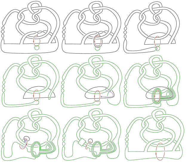
Figure 2. Computing the dual of $P$. The transition between the final two pictures is an isotopy of the green component in the complement of the other two. $P^{*}$ is given by the curve $\widehat{P}^{*}$ in the complement of a neighborhood of the red curve in the final picture.

2.1.3. A Universal Construction

Proposition 2.4.

Any pattern, $P$, constructed as follows is dualizable:

1. Pick an oriented knot $K_{0}$ in ${S}^{3}$ and draw a positively oriented meridian, $m_{0}$, around $K_{0}$.

2. Draw unoriented parallel copies of $m_{0}$, labelled $m_{1},\ldots,m_{n}$, so that all $m_{0\leq i\leq n}$ bound disjoint spanning disks.

3. Draw a band $b_{i}$ connecting $K_{0}$ to $m_{i}$ for each $1\leq i\leq n$. The bands are allowed to link in any way with $K_{0}$ and $m_{0}$, but they are not allowed to intersect each other.

4. Orient the new knot $K^{\prime}$ using the induced orientation from $K_{0}$.

5. Let $P\subset V$ be the knot $K^{\prime}\subset{S}^{3}\setminus\nu(K_{0})$.

Moreover, any dualizable pattern may be obtained from this construction by taking $K_{0}$ to be the unknot and choosing the bands correctly.

We remark that although taking the base knot to be the unknot is sufficient to produce any dualizable pattern, it is often more convenient to start with some non-trivial knot.

Proof.

Let $P$ be obtained from the process of Proposition 2.4. We start by showing that $P$ is dualizable. It suffices to give an explicit isotopy from $\widehat{P}$ to ${S}^{1}$ in $\SS 21$ by Proposition 2.2. We consider this problem in ‘dotted-circle’ diagrams. We obtain a picture of $\widehat{P}\subset\SS 21$ by drawing $K^{\prime}\cup m_{0}$ and doing 0-surgery on $m_{0}$. Since the ends of the bands $b_{*}$ are the parallel copies of $m_{0}$, we can slide each end once over the 0-surgered component $m_{0}$. Each band then retracts back onto the original knot $\widehat{K_{0}}$ so we see that $\widehat{K^{\prime}}$ is isotopic to $\widehat{K_{0}}$ in $\SS 21$. It follows from the classical light bulb theorem in $\SS 21$ that ${K^{\prime}}$ is isotopic to ${S}^{1}$ since $\mathchoice{\left\lvert\widehat{K_{0}}\cap{S}^{2}\right\rvert}{\lvert\widehat{K_{0}}\cap{S}^{2}\rvert}{\lvert\widehat{K_{0}}\cap{S}^{2}\rvert}{\lvert\widehat{K_{0}}\cap{S}^{2}\rvert}=1$.

Let $P$ be any fixed dualizable pattern. We must find a collection of bands to attach to $K_{0}=U$ as in Proposition 2.4 which recover $P$. Consider $\widehat{P}$ in the ‘dotted circle’ diagram of $\SS 21$. We know there is an ambient isotopy $\mathcal{I}:\SS 21\times[0,1]\to\SS 21$ such that $\mathcal{I}_{0}=\operatorname{Id}_{\SS 21}$ and $\mathcal{I}_{1}(\widehat{P})={S}^{1}$ by the characterization of dualizable patterns given in Proposition 2.2. Using standard techniques from Kirby calculus applied in dimension 3 to $\mathcal{I}$, we see it can be represented in the ‘dotted circle’ diagram as an alternating sequence of slides over the 0-surgered region and isotopies in the complement of the 0-surgered region. The key observation is that we can modify the isotopy in $\SS 21$ so that all the handle slides occur in sequence at the beginning, followed by an isotopy in the complement of the 0-surgered region.

We can assume the first move in the sequence associated to $\mathcal{I}$ is a handle slide without loss of generality. We proceed down the sequence until we come to the first isotopy, which we call $I_{1}$. At the end of $I_{1}$, there is a small arc on $\widehat{P}$ where the next band for the next handle slide, $S_{1}$, is attached. We can pull this arc back along $I_{1}$ and keep track of the path it traces out in $\SS 21$. It may be helpful to visualize this path as a ribbon. Since this path itself is contained in a neighborhood of an arc, we can modify $I_{1}$ so that the path intersects neither itself nor the knot $\widehat{P}$. We create a new sequence, defining a new isotopy, by removing $I_{1}$ and proceeding directly to $S_{1}$ except we append to the band the path traced out by its attaching arc under $I_{1}$, thereby defining a different slide $S^{\prime}_{1}$. The result of $S^{\prime}_{1}$ will be isotopic to the result of $S_{1}\circ I_{1}$ by an isotopy called $I^{\prime}_{1}$. We now construct a new isotopy $\mathcal{I}^{\prime}$ by removing the subsequence $I_{1}$, $S_{1}$ from $\mathcal{I}$ and replacing it with $S^{\prime}_{1}$, $I^{\prime}_{1}$. By proceeding inductively in this manner, we can create a new isotopy which consists of a sequence of slides of $\widehat{P}$ over the 0-surgered region, followed by a single isotopy in the complement.

2pt $b_{n}$ [l] at 114 153 $b_{j<n}$ [l] at 166 135 $K_{0}$ [l] at 59 28 $b_{n}^{\prime}$ [l] at 365 152

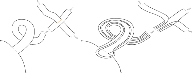
Figure 3. Resolving the intersections between the $n^{th}$ band and those of lower index.

We now have $\mathcal{I}^{\prime}$, which consists of a sequence of handle slides followed by an isotopy in the complement of the 0-surgered region. Because the slides are done one after another and not simultaneously, it is possible that the band from the $n^{th}$ slide might intersect the bands from the slides $1,\ldots,n-1$. We can fix this by resolving the intersection of each band with all those of lower index as in Figure 3. This makes the bands significantly more complicated but it ensures that they are disjoint. We can now play the isotopy backwards to see the ${S}^{1}$ factor of $\SS 21$ being simultaneously slid some number of times over the 0-surgered region to produce the curve $\widehat{P}$. This shows the existence of a sequence of bands ${b_{1},\ldots,b_{n}}$ such that if we take $K_{0}$ to be the unknot (really we should think of it as the ${S}^{1}$ factor) and attach the bands as in Proposition 2.4 then we obtain $P$. ∎

Since this construction happens in $\SS 21$, it is naturally compatible with the method we give for computing the dual pattern. Given $K_{0}$ and $b_{1},\ldots,b_{n}$, lift them to $\SS 21$, viewed as zero surgery on $m_{0}$ as before. Notice that $\lambda_{V}$ appears as a small meridian of $m_{0}$, but it does not link with the parallel copies $m_{1},\ldots,m_{n}$ which make up the ends of the bands $b_{1},\ldots,b_{n}$. We slide each band over $m_{0}$ which causes the end of each band to link once, geometrically, with $\lambda_{V}$. We retract the bands back onto $K_{0}$, which effectively attaches the same set of bands to $\lambda_{V}$. We slide $K_{0}$ over $m_{0}$ until it has become an unknot (possibly further tangling the bands now attached to $\lambda_{V}$). We slide every strand of $\lambda_{V}$ which passes through $K_{0}$ over $m_{0}$ then apply the Gluck twist (spinning the sphere composed of the obvious spanning disk for $m_{0}$ with the core of the 0-surgery) to correct the framings. A very simple example of this is given in Figure 4.

2pt $\widehat{\lambda}_{V}$ [ ] at 14 248 $m_{0}$ [ ] at 40 240 $m_{1}$ [l] at 90 211 $K_{0}$ [ ] at 94 245 $b_{1}$ [l] at 136 273 $(+2)$ [l] at 296 267 $(-2)$ [ ] at 17 107 Gluck twisting [t] at 310 16 $+2$ [ ] at 348 98 $(0)$ [ ] at 332 134 $(0)$ [ ] at 396 111 $\widehat{P}^{*}$ [l] at 433 124 $\widehat{\mu}_{V^{*}}$ [l] at 393 87 $\widehat{P}$ [ ] at 47 158

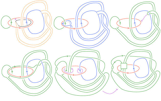
Figure 4. Working out $P^{*}$ from a base-knot-with-bands description of $P$.