MIO: Mutual Information Optimization using Self-Supervised Binary Contrastive Learning

Abstract

Self-supervised contrastive learning frameworks have progressed rapidly over the last few years. In this paper, we propose a novel mutual information optimization-based loss function for contrastive learning. We model our pre-training task as a binary classification problem to induce an implicit contrastive effect and predict whether a pair is positive or negative. We further improve the näive loss function using the Majorize-Minimizer principle and such improvement helps us to track the problem mathematically. Unlike the existing methods, the proposed loss function optimizes the mutual information in both positive and negative pairs. We also present a closed-form expression for the parameter gradient flow and compare the behavior of the proposed loss function using its Hessian eigen-spectrum to analytically study the convergence of SSL frameworks. The proposed method outperforms the SOTA contrastive self-supervised frameworks on benchmark datasets like CIFAR-10, CIFAR-100, STL-10, and Tiny-ImageNet. After 200 epochs of pre-training with ResNet-18 as the backbone, the proposed model achieves an accuracy of 86.2%, 58.18%, 77.49%, and 30.87% on CIFAR-10, CIFAR-100, STL-10, and Tiny-ImageNet datasets, respectively, and surpasses the SOTA contrastive baseline by 1.23%, 3.57%, 2.00%, and 0.33%, respectively.

1 Introduction

Self-supervised learning (SSL) has emerged as one of the pillars of its super-domain unsupervised learning. Self-supervised learning primarily aims to learn representations from data without human-annotated labels. Generally, this primary aim is fulfilled by optimizing the parameter values of the model using a pre-defined task. SSL generally consists of two phases: (1) Pre-training (or Pretext) and (2) Downstream (or target). The representations learned by the encoder in the pre-training phase are used in the downstream task in the form of transferred weights. This description gives a hint of the similarity between SSL and Transfer Learning (TL). Although the two looks similar, SSL and TL have distinct differences. The major dissimilarities between SSL and Transfer Learning (TL) can be summarised in a few words as given below.

The unlabelled dataset in the pre-training task of SSL is the same as the one used in the downstream task, whereas, in TL the pre-trained weights are obtained by training on a more diverse and large-scale annotated dataset, which differs from the one used in the downstream task too. Having a different dataset for the pre-training and the downstream task often becomes problematic, as contemporary deep learning methods require a large number of samples to yield results close to human proficiency in the target task. Researchers often adopt methods like selective fine-tuning of layers to prevent overfitting on small-scale datasets in the downstream task. However, the performance may suffer due to the destruction of the co-adaptation of the weights between the consecutive layers or from representation specificity [1]. The self-supervised learning frameworks aim to overcome this issue by pre-training on the target dataset itself. As explored in [1], fine-tuning the target dataset may improve performance, as the representation specificity no longer hampers the optimization process. The pre-training phase learns weights that provide a better initialization point for the target task as the higher-level representations become more correlated or specific to the features on the target dataset.
In past, several innovative approaches were proposed for the pre-training tasks which paved the way for efficient self-supervised representation learning. Both contrastive and non-contrastive learning approaches have succeeded in achieving state-of-the-art results on benchmark datasets. However, the ability to yield state-of-the-art performance with less annotated data requires pre-training with large models [2]. In addition to mapping feature vectors of samples from the same class or samples with similar features close to each other, self-supervised contrastive algorithms also map unlabeled dissimilar samples farther away from each other in the latent space. This characteristic of contrastive learning acts to prevent the collapse of representation in the latent space, as is often the issue in this type of learning.
In this work, we propose a novel loss function based on contrastive learning. We adopt a ground-up approach in constructing the proposed loss function. We initially adopted a pairwise binary contrastive learning approach (MIOv1) on top of which we impose a decoupling strategy to obtain a modified form (MIOv2). However, with the aid of eigen-spectrum analysis of the parameter space, we observe that optimizing the parameters of the modified form (MIOv2) is more difficult than the base version (MIOv1). Applying the concept of the Majorie-Maximization algorithm to construct the proposed loss function (MIOv3), we make the optimization process easier, which in turn gives better performance on the benchmark datasets. The main contributions of this work can be summarized as follows:

• We propose a novel loss function for contrastive self-supervised learning by modeling the pre-training task as a binary classification problem. We compare the performance of the proposed algorithm to the state-of-the-art (SOTA) self-supervised learning algorithms under the constraints of limited training periods on the task of image classification. The proposed method outperforms the SOTA methods in most cases.

• We show analytically that the proposed loss optimizes the mutual information in both positive and negative pairs.

• We present an analysis of the Hessian eigen-spectrum of the model parameters which helps to understand the optimization process of the proposed contrastive learning algorithm. To the best of our knowledge, such Hessian-based analyses have never been explored for SSL tasks.

• We also show that self-supervised learning frameworks converge to a strict saddle point for limited training.

The rest of the paper is organized as follows. In Section 1.1, we give a brief overview of the related pieces of work done in the recent past. Section 2 describes the proposed methodology. At first, it describes the base loss function and shows the relation between the mutual information and the proposed framework. This section also describes the step-by-step process of how we arrived at the proposed loss function. The section ends with a convergence analysis of self-supervised learning frameworks. In Section 3, we discuss the details of the experimental configurations that are used to establish the proof of concept. This section also analyzes the performance of the proposed loss function and compares it with the other existing self-supervised algorithms. We present an extensive analysis of the Hessian eigen-spectrum to understand the performance of the proposed framework. In Section 4, we further extend our analysis on eigen-spectrum to show the effect of decreasing the number of parameters in an SSL model. Finally, Section 5 concludes the paper.

1.1 Literature Survey

1.1.1 Self-Supervised Learning

During the initial days of self-supervised learning, a lot of techniques are designed based on handcrafted pre-training tasks, which are also known as pretext tasks. These handcrafted tasks include geometric transformation prediction [3, 4, 5], context prediction [6, 7], jigsaw puzzle solving [8, 9, 10, 11], temporal order related tasks for videos [12, 13, 14, 15, 16], pace prediction in videos [17], image colorization [18], etc. These pretext tasks are aimed at learning representations that are invariant to transformations, context, etc. Although these tasks successfully rolled the wheels of self-supervised learning, the performances of the models pre-trained with these tasks are not at par with their supervised counterparts on the target tasks.

Recently, several algorithms like SimCLR [19], MoCov1 [20], MoCov2 [21], BYOL [22], SimSiam [23], Barlow Twins [24], DCL/DCLW [25] and VICReg [26] have emerged over the course of the last few years as SSL techniques that do not require explicit pretext tasks. Some of these algorithms like SimCLR [19], MoCov1 [20], MoCov2 [21], and DCL/DCLW [25] are based on the contrastive learning principle, while others like SimSiam [23], BYOL [22], Barlow Twins [24], VICReg [26] use non-contrastive loss functions to learn representations from the data.

Self-supervised contrastive learning (SSCL) treats each data point as a separate class. Thus, a pair made of any two samples constitutes a negative pair, and a positive pair of samples is obtained by pairing two augmented versions of the same sample [27, 20, 19]. Recently, most of the SSCL-based techniques are designed by optimizing the InfoNCE [27] loss function. InfoNCE loss in contrastive learning is the same as the categorical cross-entropy loss, but the cosine similarity values between the samples in a pair are treated as logit values. Thus, InfoNCE loss can be considered the negative logarithm of the probability of predicting a positive pair. The main principle behind this learning strategy is to learn an approximate function that maps the feature vector of similar data points closer and dissimilar data points far away. The quality of representation learned by the self-supervised model is generally evaluated from the model’s performance on a $k$NN classification task using $k=200$. Recently the researchers have proposed a framework in [20, 21], that uses two networks (online and target) in the pre-training phase. The target network is momentum updated using the online network parameters to simulate a slow learning network. It also uses a memory bank to considerably increase the batch size, which proves useful in self-supervised contrastive learning by preventing representational collapse. SimCLR [19] uses large batch sizes along with sample pairing to increase the number of negative pairs in a single batch without using any memory bank. Both MoCo and SimCLR frameworks use an encoder and a non-linear multi-layered perceptron (MLP) called a projector during the pre-training phase. DCL/DCLW [25] is a recent improvement over contrastive learning frameworks. The authors showed that the performance of the SSL models can be improved by decoupling the positive and negative coupling introduced by the positive pair-related term in the denominator of the InfoNCE loss function.

In non-contrastive algorithms like SimSiam [23], BYOL [22], Barlow Twins [24], or VICReg [26], the authors use only the positive pairs for self-supervised representation learning. BYOL [22] optimizes the mean squared error between the feature vectors of the two augmented versions of a sample constituting the positive pair to ensure the invariance of representations. SimSiam [23] optimizes the negative of the cosine similarity between two samples in a positive pair. The loss function of SimSiam and BYOL is essentially the same. However, SimSiam does not use a momentum encoder like BYOL to enforce variation in the positive pair $(x_{1},x_{2})$. Instead, it uses a method called stop-gradient which prevents the back-propagation of the gradient for the projected feature vector $p_{1}$ (output taken from projector MLP) of a sample in the positive pair. The flow of gradient occurs only for the predicted feature vector $z_{2}$ (output taken from the predictor MLP) of the other sample in the positive pair. In other words, the projected feature vector $p_{1}$ is treated as a non-differentiable constant vector detached from the computational graph. Barlow Twins [24] minimizes the cross-correlation between any two feature dimensions under the assumption that each feature dimension is normally distributed. The VICReg [26] framework aims at minimizing the variance of each feature dimension to stay above a pre-defined threshold value, along with decorrelating any two feature dimensions by diagonalizing the cross-covariance matrix to prevent information collapse. The VICReg framework also uses an additional invariance term that minimizes the distance between features of the samples in a positive pair. However, the main challenges of these state-of-the-art algorithms are associated with the experimental configuration, which includes large batch sizes and memory queues, some specific momentum update routine, or the use of the stop-gradient method to avoid collapse of representation.

1.1.2 Eigen-spectrum Analysis

To the best of our knowledge, all the works on eigen-spectrum analysis in the domain of deep learning have been done on supervised frameworks. Almost all the works depend on visual aids, that is, eigenvalue versus spectral density plots to analyze the behavior of deep neural networks. In [28], we learn that the eigen-spectrum of the Hessian matrix consists of bulk and outliers. Furthermore, we also learn that we can get an estimate of the number of classes in the data from the number of outliers in the eigen-spectrum of the Hessian matrix. However, without any resource-friendly analytical method to compute all the eigenvalues of the deep neural networks with millions of parameters, it is practically intractable to obtain the full eigen-spectrum of the Hessian matrix. Hence, we have to rely on visual aid and human judgment for counting the number of outliers in the eigen-spectrum of the Hessian matrix and verify the hypothesis. Ghorbani et al. [29] on the other hand, showed that the presence of outliers in the Hessian eigen-spectrum slows down optimization. In [30], the authors observed that at the bottom of the landscape, there are a lot of eigenvalues near zero and a small number of high eigenvalues.

In [31], the author approximates the Hessian spectrum of deep networks with multi-million parameters using linear algebraic tools and showed that the eigen-spectrum consists of two parts, a bulk $H$, and outliers $G$. The work also confirmed that the bulk does not follow a Marcenko-Pastur distribution as previously believed, instead, it follows a power law trend. The work also provides evidence of the presence of a three-level hierarchical structure in the outliers $G$. However, researchers have not limited themselves to the Hessian matrix for learning about the loss landscape and the high-dimensional parameter space. In [32], the authors extend the work in [31] and explored the different parts of the eigen-spectrum to find the sources to which can be attributed. The author conjectured that the generalization of a deep network is correlated to the separation of the outliers from the bulk of the Hessian eigen-spectrum. In [33], the authors showed that the gradients span the top eigenvalues predominantly. The authors also observed that the bulk of the Hessian eigen-spectrum and the top Hessian eigenvalues are preserved over the duration of training.

2 Methodology

In this section, we propose a novel loss function for contrastive learning. First, we will discuss the motivation and the base loss function from which we derive our proposed loss function in Section 2.1. Then, we will discuss the modifications and the reason behind those to explain how we arrived at the proposed loss function in the subsequent subsections.

For the analysis we consider the self-supervised model consisting of an encoder and a non-linear projector. Let the input, encoder, encoder output (projector input), projector, and the final feature vector (output from the projector) be denoted by $x$, $f$, $h$, $q$, and $z$, respectively. The input images $x\in\mathbb{R}^{H}\times\mathbb{R}^{W}\times\mathbb{R}^{C}$ when pass through the encoder $f$, a latent vector $h\in\mathbb{R}^{F}$ is obtained. This latent vector $h$ gives the final feature vector $z\in\mathbb{R}^{D}$ when passed through the projector $g$. The loss function $\mathcal{L}_{v1}\in\mathbb{R}$ takes the feature vectors and outputs a scalar. Furthermore, let us denote the parameters of the encoder $f$ denoted by $\theta$ and that of the projector $g$ denoted by $\psi$.

To understand the flow of information we can devise the following equations

$$\begin{split}z=g_{\psi}(h)=g_{\psi}(f_{\theta}(x))\end{split}$$ (1)

2.1 MIOv1 loss function

To understand the motivation behind the proposed loss function, let us reiterate the working principle behind contrastive learning. The primary objective of the contrastive learning algorithm is to learn an approximate mapping function that maps the features of the augmented versions of a sample close to each other. For samples belonging to different classes, the feature vectors are mapped as far as possible from each other. The primary motivation of our work is based on the fact that there are only two types of pairs in contrastive learning: positive and negative. Hence, the contrastive learning principle can be seen as optimizing the distance between any two samples in the feature space. In this work, we morph the contrastive learning scenario into a binary classification problem where a pair of samples is classified either as positive and pulled closer or as negative and pushed apart. Intuitively, the base loss function named MIOv1 can be defined as given below:

$$\centering\begin{split}\mathcal{L}_{v1}=&-\mathop{\mathbb{E}}_{(x_{i},x_{j})\sim p_{+}}\left[log\left(\frac{1}{1+e^{-\frac{C_{i,j}}{\tau}}}\right)\right]\\ &-\mathop{\mathbb{E}}_{(x_{k},x_{l})\sim p_{-}}\left[log\left(1-\frac{1}{1+e^{-\frac{C_{k,l}}{\tau}}}\right)\right]\\ \end{split}\@add@centering$$ (2)

where $C_{i,j}$ is the cosine similarity between two feature vectors $z_{i}$ and $z_{j}$ obtained by passing $x_{i}$ and $x_{j}$ through the encoder and the projector. $p_{+}$ and $p_{-}$ are the distribution of positive pairs and negative pairs on $\mathbb{R}^{n}\times\mathbb{R}^{n}$, respectively and $\tau$ is the temperature parameter.

Considering $\mathcal{X}_{+}$ and $\mathcal{X}_{-}$ as the sets of positive and negative pairs sampled from the distributions of positive and negative pairs, $p_{+}$ and $p_{-}$, respectively, we can rewrite $\mathcal{L}_{v1}$ as,

$$\centering\begin{split}\mathcal{L}_{v1}=&-\frac{1}{T_{P}}\sum_{(x_{i},x_{j})\in\mathcal{X}_{+}}log\left(\frac{1}{1+e^{\frac{C_{i,j}}{\tau}}}\right)\\ &-\frac{1}{T_{N}}\sum_{(x_{k},x_{l})\in\mathcal{X}_{-}}log\left(1-\frac{1}{1+e^{-\frac{C_{k,l}}{\tau}}}\right)\\ \end{split}\@add@centering$$ (3)

We follow the same sampling procedure as in SimCLR [19]. Taking a batch size of $N$, we augment each sample in the batch to obtain two augmented samples from each sample, forming $N$ pairs and $2N$ samples in total. We can form $4N^{2}$ pairs in total, out of which $2N$ are positive pairs and $2N$ are self-pairs and these $4N$ pairs are discarded. Thus, the total number of negative pairs that can be formed is $4N^{2}-4N$. The MIOv1 loss can be expressed as follows:

$$\centering\begin{split}\mathcal{L}_{v1}=&-\frac{1}{T_{P}}\sum_{n=1}^{N}\left[ln\left(\frac{1}{1+e^{-\frac{C_{n,n^{\prime}}}{\tau}}}\right)+ln\left(\frac{1}{1+e^{-\frac{C_{n^{\prime},n}}{\tau}}}\right)\right]\\ &-\frac{1}{T_{N}}\sum_{n=1}^{2N}\sum_{\begin{subarray}{c}m=1\\ m\neq n,n^{\prime}\end{subarray}}^{2N}{ln\left(1-\frac{1}{1+e^{-\frac{C_{n,m}}{\tau}}}\right)}\\ =&-\frac{1}{N}\sum_{n=1}^{N}ln\left(\frac{1}{1+e^{-\frac{C_{n,n^{\prime}}}{\tau}}}\right)\\ &-\frac{1}{T_{N}}\sum_{n=1}^{2N}\sum_{\begin{subarray}{c}m=1\\ m\neq n,n^{\prime}\end{subarray}}^{2N}{ln\left(1-\frac{1}{1+e^{-\frac{C_{n,m}}{\tau}}}\right)}\\ \end{split}\@add@centering$$ (4)

where $n^{\prime}=n+N$, $T_{P}=2N$ and $T_{N}=4N^{2}-4N$. We can deduce a small relation between $T_{P}$ and $T_{N}$ which can be stated as $T_{N}=T_{P}^{2}-2T_{P}$. An illustrative example of how we obtain the sets of positive and negative pairs of samples is provided in Section 1 of the Supplementary.

2.2 Relation of MIOv1 loss and Mutual Information

In this subsection, we are going to derive the relationship between the MIOv1 loss function and mutual information [34, 35, 36] between the samples in a pair. The final expression of the lower bound of the MIOv1 loss function will allow us to visualize the optimization process intuitively.

Let us define the scoring function

$$s(z_{i},z_{j})=e^{C_{i,j}}$$ (5)

where $C_{i,j}$ is the cosine similarity between $z_{i}$ and $z_{j}$.

Now, the probability of the pair $(z_{i},z_{j})$ being a positive pair in a binary classification setting can be expressed as:

$$\centering\begin{split}P(pos=1|(z_{i},z_{j}))&=\frac{P_{+}(z_{i},z_{j})}{P_{+}(z_{i},z_{j})+P_{-}(z_{i},z_{j})}\\ \end{split}\@add@centering$$ (6)

Here, $P_{+}(z_{i},z_{j})$ is the probability of obtaining the positive pair $(z_{i},z_{j})$, and $P_{-}(z_{i},z_{j})$ is the probability of obtaining the negative pair $(z_{i},z_{j})$. Considering $p_{Z}(z_{i})$ as the probability of obtaining $z_{i}$ from the distribution $p_{Z}$ over all possible transformed samples of $z$ and $p_{Z,Z}(z_{i},z_{j})$ as the probability of obtaining $(z_{i},z_{j})$ from the joint distribution $p_{Z,Z}$, we deduce the following relations. When considering $(z_{i},z_{j})$ as a positive pair, the parent sample $z$ from which we obtain a positive pair is not observed. Hence, we cannot consider $z_{i}$ and $z_{j}$ as independent [37]. In Figure 1, for example, the positive transformed pair $(z_{1},z_{2})$ is obtained from the same sample $z$. Thus, $P_{+}(z_{i},z_{j})$ is equal to the probability $p_{Z,Z}(z_{i},z_{j})$. Again, when considering $(z_{i},z_{j})$ as a negative pair, there will be no dependency between the two samples, for example, $(z_{1},z_{3})$ or $(z_{2},z_{4})$ in Figure 1. Thus, $z_{i}$ and $z_{j}$ can be considered independent and $P_{-}(z_{i},z_{j})$ can be considered as the product of $p_{Z}(z_{i})$ and $p_{Z}(z_{j})$.

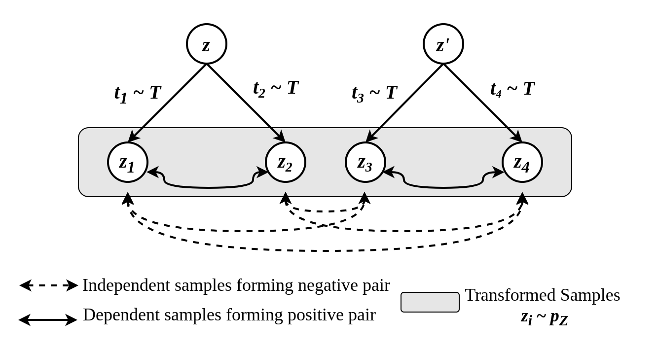
Figure 1: Graphical Model [37] showing the dependency between two samples in a positive pair and the independency between two samples forming a negative pair. Here, $z$ and $z^{\prime}$ are two different samples in a dataset. $t_{1},t_{2},t_{3},t_{4}$ are randomly chosen transformations from the distribution $T$. $z_{1}$ and $z_{2}$ are obtained by applying $t_{1}$ and $t_{2}$ on $z$. $z_{3}$ and $z_{4}$ are obtained by applying $t_{3}$ and $t_{4}$ on $z^{\prime}$.

Therefore, using the same idea, Equation 6 can be expanded as follows:

$$\centering\begin{split}P(pos=1|(z_{i},z_{j}))&=\frac{p_{Z,Z}(z_{i},z_{j})}{p_{Z}(z_{i})p_{Z}(z_{j})+p_{Z,Z}(z_{i},z_{j})}\\ &=\frac{\frac{p_{Z,Z}(z_{i},z_{j})}{p_{Z}(z_{i})p_{Z}(z_{j})}}{1+\frac{p_{Z,Z}(z_{i},z_{j})}{p_{Z}(z_{i})p_{Z}(z_{j})}}\\ \end{split}\@add@centering$$ (7)

We can also express $P(pos=1|(z_{i},z_{j}))$ in terms of $s(z_{i},z_{j})$ as follows

$$\centering\begin{split}P(pos=1|(z_{i},z_{j}))&=\frac{1}{1+e^{-C_{i,j}}}=\frac{e^{C_{i,j}}}{1+e^{C_{i,j}}}\\ &=\frac{s(z_{i},z_{j})}{1+s(z_{i},z_{j})}\\ \end{split}\@add@centering$$ (8)

Thus, comparing Equation 7 and 8, we get,

$$s(z_{i},z_{j})=e^{C_{i,j}}=\frac{p_{Z,Z}(z_{i},z_{j})}{p_{Z}(z_{i})p_{Z}(z_{j})}$$ (9)

Putting Equation 9 in Equation 2, we get,

$$\centering\begin{split}\mathcal{L}_{v1}=&-\mathop{\mathbb{E}}_{\begin{subarray}{c}(x_{i},x_{j})\sim p_{+}\end{subarray}}\left[log\left(\frac{\frac{p_{Z,Z}(z_{i},z_{j})}{p_{Z}(z_{i})p_{Z}(z_{j})}}{1+\frac{p_{Z,Z}(z_{i},z_{j})}{p_{Z}(z_{i})p_{Z}(z_{j})}}\right)\right]\\ &-\mathop{\mathbb{E}}_{\begin{subarray}{c}(x_{k},x_{l})\sim p_{-}\end{subarray}}\left[log\left(\frac{1}{1+\frac{p_{Z,Z}(z_{k},z_{l})}{p_{Z}(z_{k})p_{Z}(z_{l})}}\right)\right]\\ \geq&-\mathop{\mathbb{E}}_{\begin{subarray}{c}(x_{i},x_{j})\sim p_{+}\end{subarray}}\left[log\left(\frac{p_{Z,Z}(z_{i},z_{j})}{p_{Z}(z_{i})p_{Z}(z_{j})}\right)\right]\\ &+\mathop{\mathbb{E}}_{\begin{subarray}{c}(x_{k},x_{l})\sim p_{-}\end{subarray}}\left[log\left(\frac{p_{Z,Z}(z_{k},z_{l})}{p_{Z}(z_{k})p_{Z}(z_{l})}\right)\right]\\ \geq&-\mathop{\mathcal{I}}_{\begin{subarray}{c}(z_{i},z_{j})\sim p_{+}\end{subarray}}(z_{i},z_{j})+\mathop{\mathcal{I}}_{\begin{subarray}{c}(z_{k},z_{l})\sim p_{-}\end{subarray}}(z_{k},z_{l})\\ \end{split}\@add@centering$$ (10)

From Equation 10, we can infer that the proposed loss function $\mathcal{L}_{v1}$ works by maximizing the mutual information between the samples in a positive pair $(z_{i},z_{j})$. It also minimizes the mutual information between the samples in a negative pair $(z_{k},z_{l})$.

An intuitive explanation behind the working principle of the MIOv1 loss function is that when the samples in a negative pair belong to the same underlying category, the encoder learns only the common representations between them, including both low and high-level representations. The mutual information is the least when the two samples in a negative pair belong to two different classes. In that case, the encoder should learn only the common low-level representations among all the samples in the dataset. High-level representations are better learned when the mutual information is maximized for samples in a positive pair.

2.3 Effect of Removing a Repulsive Force

We can expand Equation 4, to get,

$$\centering\begin{split}\mathcal{L}_{v1}=&-\frac{1}{N}\sum_{n=1}^{N}ln\left(\frac{1}{1+e^{-\frac{C_{n,n^{\prime}}}{\tau}}}\right)\\ &-\frac{1}{T_{N}}\sum_{n=1}^{2N}\sum_{\begin{subarray}{c}m=1\\ m\neq n,n^{\prime}\end{subarray}}^{2N}{ln\left(1-\frac{1}{1+e^{-\frac{C_{n,m}}{\tau}}}\right)}\\ =&-\frac{1}{N}\sum_{n=1}^{N}{\frac{C_{n,n^{\prime}}}{\tau}}+\frac{1}{N}\sum_{n=1}^{N}{ln\left(1+e^{\frac{C_{n,n^{\prime}}}{\tau}}\right)}\\ &+\frac{1}{T_{N}}\sum_{n=1}^{2N}\sum_{\begin{subarray}{c}m=1\\ m\neq n,n^{\prime}\end{subarray}}^{2N}{ln\left({1+e^{\frac{C_{n,m}}{\tau}}}\right)}\\ \end{split}\@add@centering$$ (11)

where $n=n+N$ and $T_{N}$ bear the same meaning as in Equation 4. In the Equation 11, we see that minimizing the loss $\mathcal{L}_{v1}$, minimizes the second and term in the last line. This means that the terms $C_{n,n^{\prime}}$ and $C_{n,m}$ are also minimized. However, $C_{n,m}$ being the cosine similarity of the samples in a positive pair should be maximized to $+1$. We see that a repulsive force will take effect on the samples in the positive pair due to the minimization of the second term in the last line of Equation 11.

Initially, we hypothesized that eliminating this repulsive force would improve the performance and result in faster convergence in the optimization process. This leads us to derive our second loss as mentioned in Equation 12. We call this loss function MIOv2.

$$\centering\begin{split}\mathcal{L}_{v2}=&-\frac{1}{N}\sum_{n=1}^{N}{\frac{C_{n,n^{\prime}}}{\tau}}+\frac{1}{T_{N}}\sum_{n=1}^{2N}\sum_{\begin{subarray}{c}m=1\\ m\neq n,n^{\prime}\end{subarray}}^{2N}{ln\left({1+e^{\frac{C_{n,m}}{\tau}}}\right)}\\ \end{split}\@add@centering$$ (12)

The above equation can also be written as,

$$\centering\begin{split}\mathcal{L}_{v2}=&-\mathbb{E}_{(x_{i},x_{j})\sim p^{+}}\left[\frac{C_{i,j}}{\tau}\right]+\mathbb{E}_{(x_{k},x_{l})\sim p^{-}}\left[ln\left(1+e^{\frac{C_{k,l}}{\tau}}\right)\right]\\ \end{split}\@add@centering$$ (13)

where $p_{+}$ and $p_{-}$ denote the same quantities as in Equation 4. However, as evident from the experimental results presented in Section 3.3, we can see that optimizing the model parameters using $\mathcal{L}_{v1}$ yields better kNN accuracy than $\mathcal{L}_{v2}$. This behavior is counter-intuitive to what our hypothesis stated. In the following subsection, we explore the explanation for such behavior.

2.4 Improving Performance by Optimizing a Surrogate Function

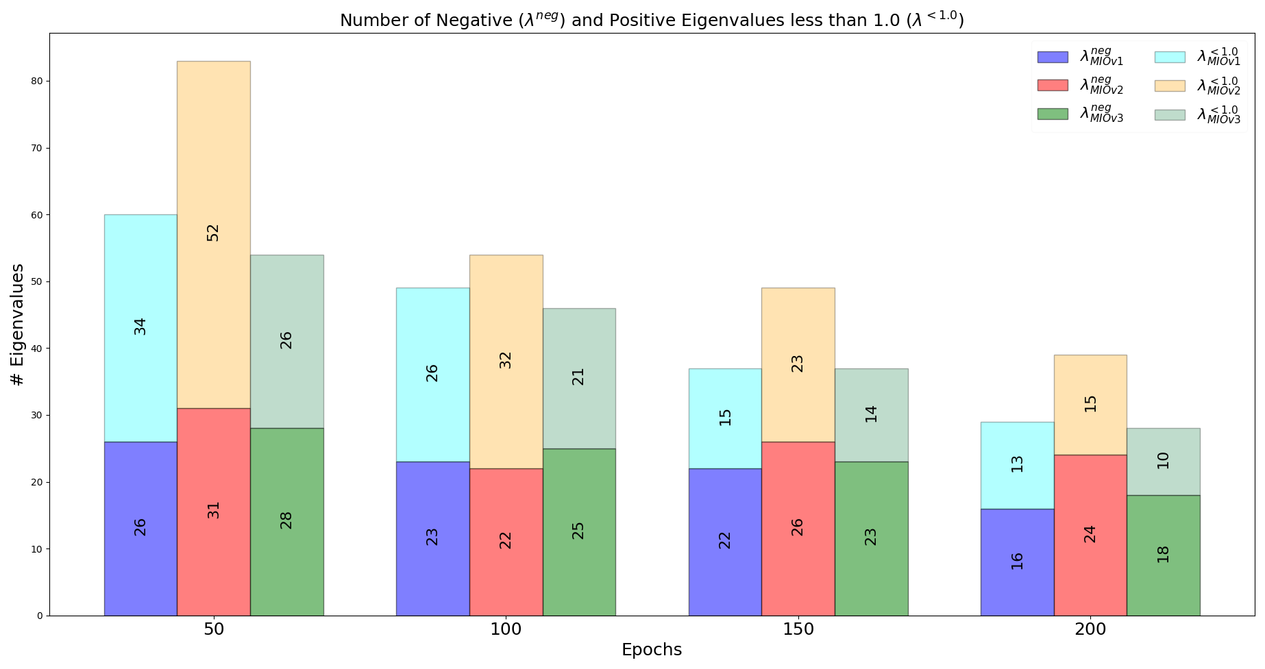
Figure 2: Comparison of Negative ($\lambda^{neg}$) and Positive Eigenvalues with values less than 1 ($\lambda^{<1.0}$) for MIOv1 and MIOv2. The figure is best visible at 300%.

Due to degradation in performance when using $\mathcal{L}_{v2}$ (refer to Table II), we consider modifying it further to improve the performance. The reason behind the degradation of performance can be attributed to the difficulty in the optimization of $\mathcal{L}_{v2}$. This is evident from the eigen-spectrum plot given in Figure 2 and also in Figure 3. Without loss of generosity, we consider eigen-directions with eigenvalues less than $1.0$ to be flat, as the optimal step size along those directions is high $(\eta>1.0)$ compared to the learning rate at any step, the progress along those directions is very slow compared to the eigen-directions with larger eigenvalues. Thus, we can also observe that the eigen-spectrum of MIOv2 contains more eigenvalues near zero than MIOv1, which indicates that the loss landscape of MIOv2, that is, $\mathcal{L}_{v2}(g_{\psi}(f_{\theta}(X)))$ has more number of flat eigen-directions than MIOv1, that is, $\mathcal{L}_{v1}(g_{\psi}(f_{\theta}(X)))$. This causes the optimization to be harder in the case of $\mathcal{L}_{v2}(g_{\psi}(f_{\theta}(X)))$ than $\mathcal{L}_{v1}(g_{\psi}(f_{\theta}(X)))$. A zero eigenvalue also indicates that the current parameter state contains an inflection point along the corresponding eigen-direction. Optimizing along such an eigen-direction is also difficult if the learning rate is low and the optimizer is trying to escape local minima.

Figure 3: eigen-spectrum comparison for MIOv1, MIOv2 and MIOv3. Spectral Density vs Eigenvalue plot for MIOv1, MIOv2, and MIOv3. The figure was obtained after executing 100 iterations of the Lanczos Tridiagonalization algorithm. The pre-trained ResNet18 models were trained using an SGD optimizer with a learning rate of 0.06, cosine annealing decay, and a batch size of 128 on the CIFAR-10 dataset. The eigen-spectrum was computed with the model weights obtained after 200 epochs of pre-training. The figure is best viewed at 300%.

2.4.1 Non-Convexity of MIOv1 and MIOv2

The eigenvalues of the Hessian matrix $\mathcal{H}$ determine the nature of the critical points. If along the direction of any eigenvector $v$, the value of the quantity $v^{T}\mathcal{H}v<0$, then it can be concluded that the function representing the mapping of the input pair space $\chi$ to the output space, i.e. $(\mathcal{L}_{v1/v2}\circ g_{\psi}\circ f_{\theta}):\chi\rightarrow\mathbb{R}$, is non-convex and the non-convexity is encountered along the direction of the eigenvector $v$. The aforementioned statement can be justified by the fact that any twice differentiable function is convex if and only if its domain is convex and the Hessian of the function is a positive semi-definite matrix for all values in its domain [38].

We observe from Figure 3, that all the SSL loss functions contain negative eigenvalues. Hence, it can be concluded that the loss landscape generated by these loss functions is non-convex in nature.

2.4.2 MIOv3 Loss Function

According to Majorize-Minimization Algorithm [39], the extremum value of a function that is difficult to optimize, e.g., $\mathcal{L}_{v2}(z)$ can be achieved by optimizing a surrogate function $\mathcal{L}_{v3}(z)$, where

$$\centering\begin{split}\mathcal{L}_{v3}(z|z_{k})&\geq\mathcal{L}_{v2}(z)\;\forall\;z\in\mathcal{Z}\;\text{and}\\ \mathcal{L}_{v3}(z|z_{k})&=\mathcal{L}_{v2}(z_{k})\\ \end{split}\@add@centering$$ (14)

where $z\in\mathcal{Z}$ (latent space of the projector) and $z_{k}\in\mathcal{Z}$ is the projected latent vector at any given time step $k$. We intend to take the Majorize of the MIOv2 loss function $\mathcal{L}_{v2}$ in Equation 13, by taking the upper bound of the second term in the equation. Using Mean Value Theorem [40], there exists $\xi\in(0,x)$, such that,

$$\centering\begin{split}ln(1+x)=ln(1+x)-ln(1)&=x\cdot\left[\frac{\partial ln(1+x)}{\partial x}\right]_{x=\xi}\\ &=x\cdot\frac{1}{1+\xi}\leq x\\ \end{split}\@add@centering$$ (15)

Using the above relation in $ln\left(1+e^{\frac{C_{k,l}}{\tau}}\right)$ from Equation 13, we get,

$$\centering\begin{split}ln\left(1+e^{\frac{C_{k,l}}{\tau}}\right)\leq e^{\frac{C_{k,l}}{\tau}}\\ \end{split}\@add@centering$$ (16)

Replacing $ln\left(1+e^{\frac{C_{k,l}}{\tau}}\right)$ by $e^{\frac{C_{k,l}}{\tau}}$ in Equation 13, we get,

$$\centering\begin{split}\mathcal{L}_{v3}=&-\mathbb{E}_{(x_{i},x_{j})\sim p^{+}}\left[\frac{C_{i,j}}{\tau}\right]+\mathbb{E}_{(x_{k},x_{l})\sim p^{-}}\left[e^{\frac{C_{k,l}}{\tau}}\right]\\ =&-\sum_{(x_{i},x_{j})\in\mathcal{X}^{+}}\left[\frac{C_{i,j}}{\tau}\right]+\sum_{(x_{k},x_{l})\in\mathcal{X}^{-}}\left[e^{\frac{C_{k,l}}{\tau}}\right]\\ \end{split}\@add@centering$$ (17)

We can rewrite the above equation as,

$$\centering\begin{split}\mathcal{L}_{v3}=&-\frac{1}{N}\sum_{\begin{subarray}{c}n=1\end{subarray}}^{N}\frac{C_{n,n^{\prime}}}{\tau}+\frac{1}{T_{N}}\sum_{\begin{subarray}{c}n=1\end{subarray}}^{2N}\sum_{\begin{subarray}{c}m=1\\ m\neq n,n^{\prime}\end{subarray}}^{2N}e^{\frac{C_{n,m}}{\tau}}\\ \end{split}\@add@centering$$ (18)

where $n^{\prime}=n+N$, $T_{N}=2N(2N-2)$ for a batch of size $N$. $\mathcal{X}_{+}$ and $\mathcal{X}_{-}$ are sets of positive and negative pairs of samples obtained from the distribution of positive and negative pairs, $p_{+}$ and $p_{-}$, respectively. We call this version of the loss as MIOv3, that is, $\mathcal{L}_{v3}(g_{\psi}(f_{\theta}(X)))$, which is our final proposed loss function. Pre-training a ResNet18 model on CIFAR-10 using the same hyper-parameters configuration as MIOv1 and MIOv2 in Figure 3, we observe that the performance improves considerably and even surpasses the contemporary contrastive learning frameworks on CIFAR-10. The comparison of the eigen-spectrums of MIOv1, MIOv2, and MIOv3 loss functions is shown in Figure 3. Out of the 100 eigenvalues, the range of eigenvalues extends well beyond the highest eigenvalue of Hessian of the weights of MIOv1 and MIOv2 models. The number of positive eigenvalues near zero $(<1.0)$ after 200 epochs of training is also less for MIOv3 ($\lambda_{<1.0}=10$) than for MIOv1 ($\lambda_{<1.0}=13$) and MIOv2 ($\lambda_{<1.0}=15$). We argue that even having a few more negative eigenvalues, the number of near-zero positive eigenvalues compensates for the obstructive effect faced in those eigen-directions having negative eigenvalues. In other words, the flat directions are less for MIOv3 than MIOv1, and convexities are also stronger for MIOv3 than MIOv1. This leads to better optimization, and consequently, better performance for MIOv3. We will discuss further on this topic in Section 3.3, where we will analyze intermediate eigen-spectrums of the training phase to get an insight into the proposed self-supervised optimization process.

2.5 Do SSL methods converge?

The loss landscape of the different models in the frameworks depends on the loss function used. The loss functions shape the loss landscape as a function of the parameter space $\mathbb{P}$. The input pair space $\chi$ is mapped to the latent space $\mathbb{R}^{D}$ by a function $g_{\psi}\circ f_{\theta}$ or $(g\circ f)_{\mathcal{P}}$, where $\mathcal{P}=\{\theta,\psi\}$ denotes a point in the parameter space $\mathbb{P}$. The paired latent vectors obtained from the function $g_{\psi}\circ f_{\theta}$ or $(g\circ f)_{\mathcal{P}}$, in the self-supervised pre-training phase, constitute a joint embedding space $\mathcal{E}:\mathbb{R}^{D}\times\mathbb{R}^{D}$ and is mapped to the loss landscape $\mathbb{L}$ through the projector loss function $\mathcal{L}$.

$$\mathcal{L}\circ(g\circ f)_{\mathcal{P}}:\chi\rightarrow\mathbb{L}$$ (19)

As the learning rate decreases, the conditions become more favorable for the descent into a convex valley in the loss landscape. However, decreasing the learning rate deters the optimizer from proceeding with the same ease in the flat plateaus or at inflection points to escape local minima. To ensure convergence along the steepest eigen-direction, it is necessary to have a learning rate $\eta\leq\frac{1}{L}=\frac{1}{\lambda_{max}}$ [41].

Rewriting the Polyak-Lojasiewicz Inequality (Section 6 in Supplementary) in terms of non-convex loss function $\mathcal{L}$, for $\mu>0$ the global linear convergence rate is given by

$$\centering\begin{split}\mathcal{L}(w_{k})-\mathcal{L}^{*}\leq(1-\frac{\mu}{L})^{k}(\mathcal{L}(w_{0})-\mathcal{L}^{*})\\ \end{split}\@add@centering$$ (20)

, where $w_{k},w_{0}$ are the parameter state at the $k^{th}$ and $0^{th}$ step.

If we consider convergence along each eigen-direction, we can calculate the expected convergence rate over the whole of the loss landscape. Considering a single eigen-direction corresponding to eigenvalue $\lambda_{i}$, the above equation reduces to,

$$\centering\begin{split}\mathcal{L}(w^{i}_{k})-\mathcal{L}^{*}(w^{i})\leq(1-\frac{\mu_{i}}{\lambda_{i}})^{k}(\mathcal{L}(w^{i}_{0})-\mathcal{L}^{*}(w^{i}))\\ \end{split}\@add@centering$$ (21)

subject to the satisfiability of

$$\centering\begin{split}\frac{1}{2}\lVert\nabla\mathcal{L}^{i}(w)\rVert^{2}\geq\mu_{i}(\mathcal{L}^{i}(w)-\mathcal{L}^{*})\end{split}\@add@centering$$ (22)

The left-hand side of equation Equation 22 is always positive but the magnitude depends on the curvature along the eigen-direction. The right-hand side is also always positive as in the case of stable loss minimization $\mathcal{L}^{*}<\mathcal{L}^{i}(w)$ at any optimization step. The Equation 22 is not satisfied for critical points, except at global minima. In all other cases, the PL Inequality will be satisfied for any scalar $\mu>0$. However, we can still calculate a pseudo convergence rate by considering the satisfiability of Equation 22 at critical points along some eigen-directions in the limiting sense, i.e.

$$\frac{1}{2}lim_{\nabla\rightarrow 0}\lVert\nabla\mathcal{L}^{i}(w)\rVert^{2}_{\nabla\approx 0}\geq lim_{\mu_{i}\rightarrow 0^{+}}\mu_{i}(\mathcal{L}^{i}(w)-\mathcal{L}^{*})$$ (23)

We take an expectation over all the eigen-directions to calculate a proxy for the linear convergence rate.

$$\centering\begin{split}\mathbb{E}_{i}\left[\mathcal{L}(w^{i}_{k})-\mathcal{L}^{*}(w^{i})\right]&\leq\mathbb{E}_{i}\left[(1-\frac{\mu_{i}}{\lambda_{i}})^{k}(\mathcal{L}(w^{i}_{0})-\mathcal{L}^{*}(w^{i}))\right]\\ &\leq\mathbb{E}_{i}\left[(1-\frac{\mu_{i}}{\lambda_{max}})^{k}(\mathcal{L}(w^{i}_{0})-\mathcal{L}^{*}(w^{i}))\right]\\ &\leq\mathbb{E}_{i}\left[(1-\frac{\mu_{i}}{L})^{k}(\mathcal{L}(w^{i}_{0})-\mathcal{L}^{*}(w^{i}))\right]\\ &\leq\mathbb{E}_{i}\left[(1-\frac{\mu_{min}}{L})^{k}(\mathcal{L}(w^{i}_{0})-\mathcal{L}^{*}(w^{i}))\right]\\ &\leq\mathbb{E}_{i}\left[c^{k}(\mathcal{L}(w^{i}_{0})-\mathcal{L}^{*}(w^{i}))\right]\leq\delta^{\prime}\\ \end{split}\@add@centering$$ (24)

where $c^{k}=(1-\frac{\mu_{min}}{L})^{k}\rightarrow 0$ if $k\rightarrow\infty$.

From Equation 24, we can see that the convergence rate becomes infinitesimal for a large value of $k$, that is, for a long training process. However, we will look into Eqn. (6.11) of the Supplementary, where we derive an expression of the expected gradient norm, as

$$\centering\begin{split}\sum_{t=1}^{T}\left(\eta_{t}-\frac{\eta_{t}^{2}L}{2}\right)\mathbb{E}_{t}\left[\lVert\nabla f(x_{t})\rVert_{2}^{2}\right]&\leq\mathcal{L}(w_{k})-\mathcal{L}^{*}+\frac{\sigma^{2}L}{2}\sum_{t=1}^{T}\eta_{t}^{2}\\ \end{split}\@add@centering$$

, where we have assumed that the variance of the stochastic gradient is bounded above by $\sigma^{2}$.

Putting the expression for the proxy of the convergence rate in place of $\mathcal{L}(w_{i})-\mathcal{L}^{*}$, we get,

$$\centering\begin{split}&\sum_{t=1}^{T}\left(\eta_{t}-\frac{\eta_{t}^{2}L}{2}\right)\mathbb{E}_{t}\left[\lVert\nabla f(x_{t})\rVert_{2}^{2}\right]\\ &\leq\mathbb{E}_{i}\left[\mathcal{L}(w^{i}_{k})-\mathcal{L}^{*}(w^{i})\right]+\frac{\sigma^{2}L}{2}\sum_{t=1}^{T}\eta_{t}^{2}<\infty\\ \end{split}\@add@centering$$ (25)

where, $\eta_{t}$ varies with time as $\eta_{t}=\eta_{min}+\frac{1}{2}(\eta_{max}-\eta_{min})\left(1+\cos\left(\frac{t}{T}\pi\right)\right)$ with $\eta_{min}=0$, and $T$ is the total number of steps. From the expression of $\eta_{t}$, we have,

$$\begin{split}\sum_{t=1}^{\infty}\eta_{t}\to\infty\text{ and }\sum_{t=1}^{\infty}\eta_{t}^{2}<\infty\\ \end{split}$$ (26)

From Equation 24 and 25, we calculate a proxy for the linear convergence rate and deduce that longer training results in convergence. However, combining our deduction with the Hessian eigen-spectrum, we can conclude that for limited training, the convergence does not occur to any local minima. In fact, the convergence point after 200 epochs (and every point in parameter space during the course of training) is a strict saddle point, i.e., $\lambda_{min}<0$. Please refer to Section 6 of the Supplementary for more details.

3 Experiments and Results

In this section, first, we are going to discuss the datasets that we used for our experiments, and then the experimental configuration of the models we used. We also present the accuracies of the proposed framework on the mentioned datasets and compare them with the state-of-the-art algorithms.

3.1 Datasets

We use four popular datasets to conduct the experiments, namely, CIFAR-10, STL-10, CIFAR-100, and Tiny ImageNet. The dimensions of images in CIFAR-10, STL-10, CIFAR-100 and Tiny ImageNet are $32\times 32$, $96\times 96$, $32\times 32$ and $64\times 64$, respectively. The details of the distribution of the training and test sets are given in Table I.

TABLE I: Training and Test images distribution in different datasets

Dataset	No. of	Images		Image
	classes	Training	Test	Dimensions
CIFAR-10	10	50000	10000	32 $\times$ 32
CIFAR-100	100	50000	10000	32 $\times$ 32
STL-10	10	5000	8000	96 $\times$ 96
Tiny Image Net	200	100000	10000	64 $\times$ 64

3.2 Implementation Details

In this section, we mention the configuration of the best-performing models for the listed frameworks. The frameworks were implemented using the lightly-ai [42] library. All the models were trained using ResNet-18 with a batch size of 128 The respective loss functions of the self-supervised models were optimized using an SGD optimizer with a learning rate of 0.06 for CIFAR10 and CIFAR100, and a learning rate of 0.03 for STL-10 and Tiny-ImageNet. The models were pre-trained for short training periods of 200 epochs only.

We decayed the learning rate following a cosine annealing schedule. The value of weight decay used is $5\times 10^{-4}$. The ResNet architecture is modified as mentioned in [19] only for CIFAR10 and CIFAR100 datasets as the image dimensions are $32\times 32$.

For MIOv1, MIOv2, and MIOv3, we used a temperature value of $0.2$. Whereas for SimCLR [19], DCL [25], and DCLW [25], we used a temperature of $0.1$ as recommended in the paper [25]. For MoCov2 [21], we used a temperature value of $0.07$, as recommended in its paper. The same value of temperature hyper-parameter value does not yield the best performance for all the frameworks on a particular dataset. Hence, we use a temperature value that yields the best performance for the respective frameworks.

3.3 Results and Analysis

In this subsection, we present the results of frameworks with MIOv1, MIOv2, and the proposed MIOv3 loss function along with the contrastive frameworks SimCLR, MoCOv2, SimCLR+DCL, SimCLR+DCLW and the non-contrastive frameworks BYOL, Barlow Twins. All the frameworks were trained and evaluated using a $k$NN classifier with $k=200$ on four datasets as mentioned in 3.1. The Top-1 200-NN accuracy values are given in Table II.

TABLE II: 200-NN evaluation results on CIFAR-10, CIFAR-100, STL-10 and Tiny ImageNet-200 datasets of SimCLR, MoCoV2, DCL, DCLW, Barlow Twins, BYOL, MIOv1, MIOv2 and MIOv3 frameworks. The configuration and implementation details for each experiment are mentioned in Section 3.2.

Frameworks	Contrastive				Non-Contrastive		Binary Contrastive
	SimCLR	MoCoV2	SimCLR+DCL	SimCLR+DCLW	Barlow Twins	BYOL	MIOv1	MIOv2	MIOv3
Dataset	CIFAR-10
200-NN Accuracy (%)	81.23	83.73	84.97	84.29	84.03	86.84	81.26	81.14	86.2
Dataset	CIFAR-100
200-NN Accuracy (%)	54.2	54.35	54.24	54.61	53.04	54.02	50.78	47.10	58.18
Dataset	STL-10
200-NN Accuracy (%)	75.65	75.64	74.46	75.49	73.24	75.87	73.66	72.58	77.49
Dataset	Tiny ImageNet-200
200-NN Accuracy (%)	24.64	29.41	29.23	30.54	27.42	21.21	27.59	15.6	30.87

3.4 Eigen-spectrum Visualization and Analysis

(a) Eigen-spectrum comparison of MIOv3, SimCLR, Barlow Twins frameworks on CIFAR-10

(b) Eigen-spectrum comparison of MIOv3, SimCLR, SimCLR+DCL, SimCLR+DCLW frameworks on CIFAR-10

(c) Eigen-spectrum comparison of MIOv3, SimCLR+DCL, BYOL frameworks on CIFAR-10

Figure 4: Eigen-spectrum of all the frameworks used in comparison with our proposed framework, in reference to MIOv3. The frameworks used in this figure, apart from MIOv3, are SimCLR, Barlow Twins, SimCLR+DCL, SimCLR+DCLW, and BYOL. The eigen-spectrum was constructed using 100 eigenvalues obtained using the weights after 200 epochs of self-supervised pre-training.

In Section 2.4, we have shown the eigen-spectrum plot in Figure 3, and explained the reason for the improvement in performance in MIOv3 and degradation of performance in MIOv2, compared to MIOv1. To reiterate, although all three frameworks showed a bulk of eigenvalues near zero, which indicates flat curvature or inflection point along the direction of the corresponding eigenvectors, we observed that as we move towards higher positive eigenvalues, the spectral density is greater for MIOv3 for most of the shown interval. The magnitude of positive eigenvalues denotes the sharpness of convexity in the corresponding eigen-directions (i.e., directions along the eigenvectors). This indicates that the final parameter state $\mathcal{P}^{v3}_{T}$ of MIOv3 contains more sharp convex eigen-directions, where $T$ is the total number of training steps. On the other hand, the presence of more flat eigen-directions or inflection points along the path of optimization in the parameter space $\mathbb{P}^{v1}$ and $\mathbb{P}^{v2}$, of MIOv1 and MIOv2, respectively, makes reaching a local minimum difficult.

In this section, we will further expand our analysis to other contemporary frameworks and try to provide an explanation behind the observed behavior of our proposed frameworks. In relation to the study, it should be mentioned that the Hessian matrix contains information about the curvature of the loss landscape, and studying its eigen-spectrum gives us a profound idea of it. This helps us in drawing informed conclusions about the state of the optimization process and the nature of the convergence.

From Table II, we see that the proposed framework MIOv3 outperforms the state-of-the-art contrastive learning frameworks and also performs at par with other state-of-the-art self-supervised frameworks. However, from the Hessian eigen-spectrum plots in Figure 4, we observe that the Hessian eigen-spectrum of none of the frameworks satisfies the Hurwicz Local Minimizer criteria, i.e., $\nabla^{2}(\mathcal{L}\circ g_{\psi}\circ f_{\theta})>0$. In other words, none of the frameworks are at a local minimum. This eliminates the question of convergence to local minima for any of the frameworks used in our study.

In fact, from Figure 4b, we can observe that the Hessian eigen-spectrum of SimCLR+DCL and SimCLR+DCLW contains a large number of positive eigenvalues with a magnitude greater than all but one eigenvalues of MIOv3, but fails to outperform not only on CIFAR10 dataset but also on all the other datasets used in our experiments. Again, suppose we carefully observe the Hessian eigen-spectrum of BYOL in Figure 4c. In that case, we can see that the Hessian eigen-spectrum of BYOL contains a number of positive eigenvalues with very high magnitude $(>200)$. Intuitively and mathematically, this denotes very sharp convexity around the point in the parameter space $\mathbb{P}$. At this point of the discussion, it is worth noting that the number of negative eigenvalues in the Hessian eigen-spectrum of BYOL, DCL, and DCLW is less than half of that in the Hessian eigen-spectrum of MIOv3. All the above evidences suggest that the proportion of sharp convex eigen-directions is more in number for DCL, DCLW, and BYOL than MIOv3. But, MIOv3 outperforms DCL and DCLW and falls behind BYOL only by $0.64\%$, which we believe can be overcome by hyper-parameter tuning or changing the initialization seed.

From the eigen-spectrum plots in Figure 4, we observe a large peak around zero in the Hessian eigen-spectrum of all the frameworks. This establishes the fact that the loss landscape consists of flat plateaus and directions with low curvature around the current point in the parameter space $\mathbb{P}$. Local minima are likely to have an error very close to a global minimum. Furthermore, a global minimum is surrounded by positive curvature along all eigen-directions. However, we see no such properties in the Hessian eigen-spectrum of any of the frameworks. This phenomenon is also observed for other datasets like CIFAR-100 and Tiny ImageNet-200. In Figure 5, we present the eigenspectrum of all versions of the MIO loss function and the second-best performing frameworks on the respective datasets. We also observe that the eigenspectrum follows the same pattern as for the CIFAR-10 dataset. Thus, we can conclude that none of the frameworks achieve convergence after limited training of 200 or even 500 epochs, as evident from Figure 6.

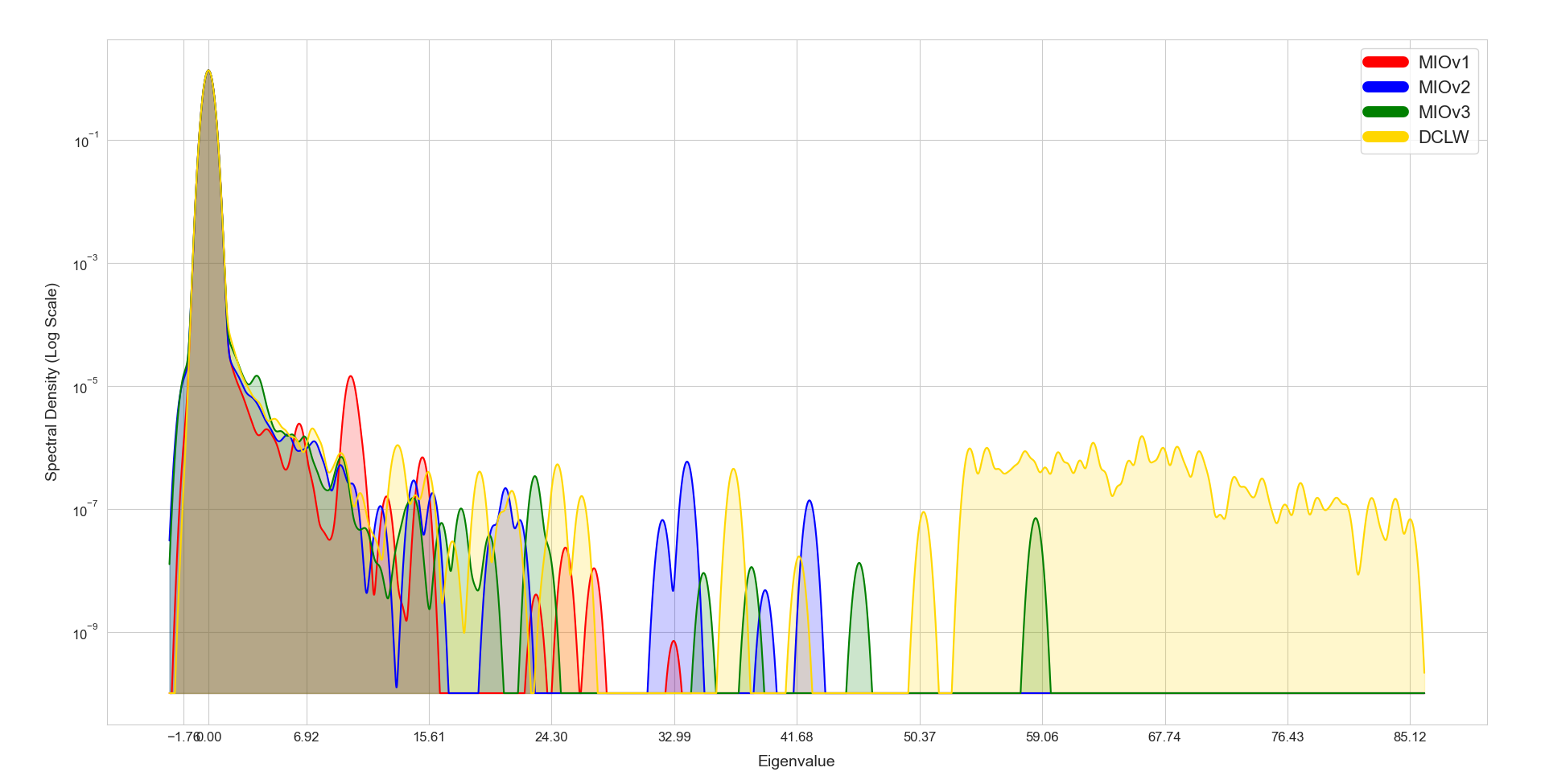
(a) Eigen-spectrum comparison on CIFAR-100

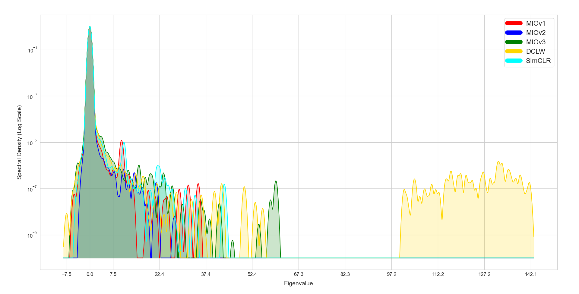
(b) Eigen-spectrum comparison on Tiny ImageNet-200

Figure 5: Eigenspectrum of all versions of MIO framework and the second-best performing frameworks on CIFAR100 and Tiny ImageNet-200 datasets.

3.4.1 What can we say about the frameworks from the eigen-spectrum?

(a) Eigen-spectrum comparison of MIOv3 from 100th to 500th epoch on CIFAR-10

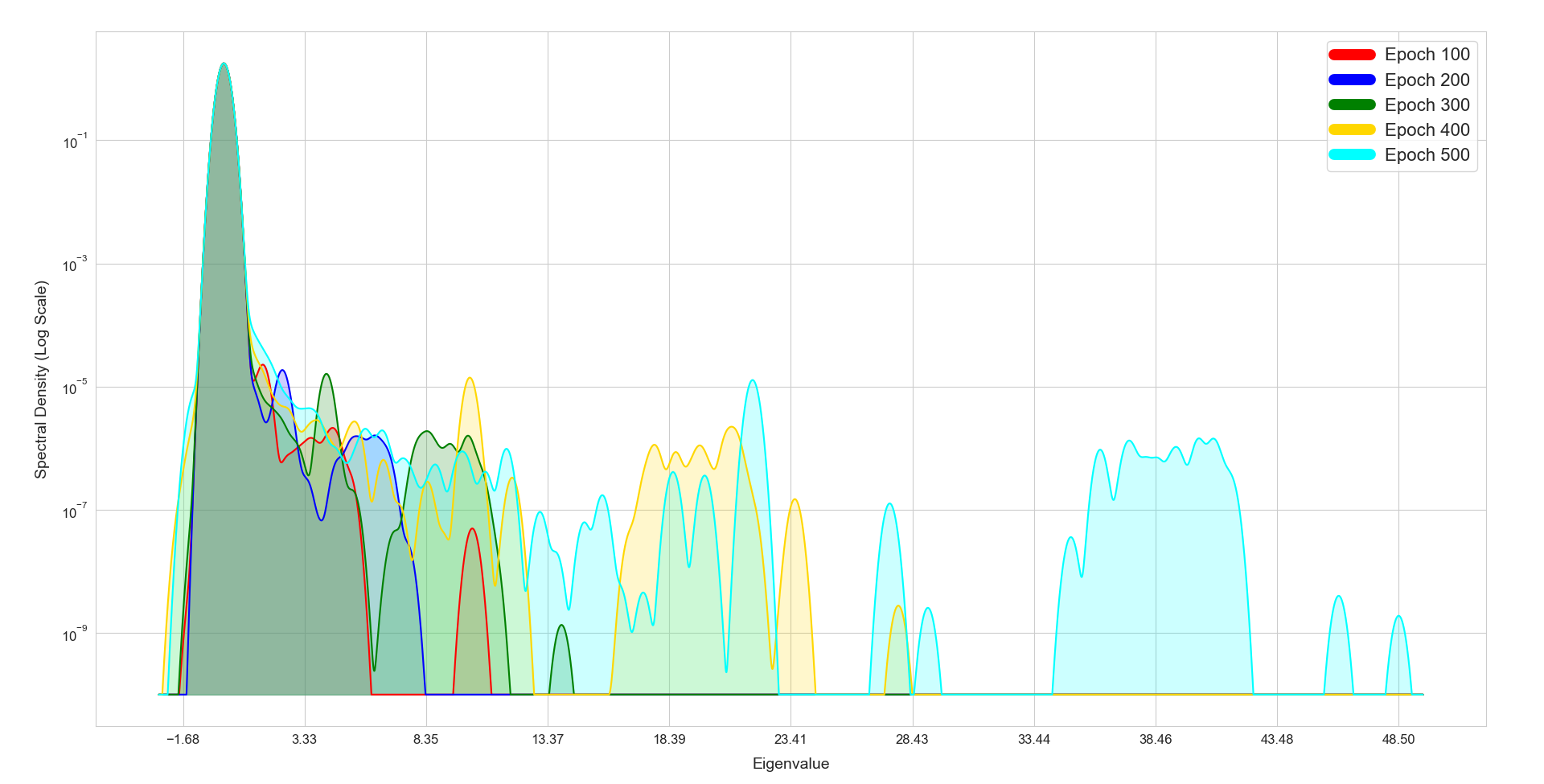
(b) Eigen-spectrum comparison of SimCLR from 100th to 500th epochs on CIFAR-10

Figure 6: Eigen-spectrum of MIOv3 and SimCLR frameworks used in comparison with our proposed framework, in reference to MIOv3. Figures are best visible at 300% scale.

In this section, our primary objective is to explore the path taken by the optimization process to reach the final parameter state $\mathcal{P}_{T}$, where $T$ is the total number of training iterations or steps. From Figure 6, we are able to observe the change in the Hessian eigen-spectrum over the course of pre-training from the $100^{th}$ to the $500^{th}$ epoch at an interval of 100 epochs. The eigen-spectrum at each step gives us information about the neighborhood of the parameter state $\mathcal{P}_{t}$ at any training step $t$. For example, in the case of SimCLR (Figure 6b), we observe that the Hessian eigen-spectrum consists of two bulk regions in the eigen-spectrum. We can observe that, as the training progresses, the secondary bulk moves towards higher eigenvalues. This indicates that as the training progresses, the model is able to find sharper minima along some eigen-directions. Eigen-spectrum of DCL and BYOL is provided in Section 5 of the supplementary material to support the aforementioned statements.

From the eigen-spectrum plots in Figure 3, 5, and 6, we can see that the final parameter state of all the frameworks converges to a non-optimal strict saddle point. The optimization process does not converge to a strict convex point in the parameter space. Thus, it can be concluded that SSL frameworks lead to premature convergence.

4 Ablation Studies

In this ablation study, we mainly discuss the effect of the number of parameters on performance. The presence of a bulk of eigenvalues around zero only indicates that a bulk of the eigen-directions are flat or are inflection points. At a low learning rate, little change will occur to the parameters contributing to the flat eigen-directions. If some particular eigen-direction is flat, it allows the current parameter state to move around the neighborhood of the parameter state in the flat eigen-direction, without much change in the loss value, at low values of learning rate. So, any state in the parameter space $\mathcal{P}_{t}$ with flat eigen-directions basically can be considered as a quotient space $\mathcal{P}^{q}_{t}$, where the equivalence relation is on the set of parameters along a particular eigen-direction, which causes little change in the loss value, i.e., $\mathcal{P}_{t}\rightarrow\mathcal{P}^{q}_{t}\setminus\{W:\mathcal{L}^{\{w_{1}\}}-\mathcal{L}^{\{w_{2}\}}<\epsilon\;\forall w_{1},w_{2}\in W\}$. In other words, we can also say that there exists a basin along some particular flat eigen-direction. However, the eigenvalue may change along the eigen-direction over the course of training depending on the learning rate, and the current parameter state may move from a flat basin to an inflection point and further to an optimum.

Since the loss is not optimized along these directions, we can say that the non-trivial parameter subspace $\mathbb{P}_{\nabla\neq 0}$ which aids in loss optimization is smaller than the original parameter space $\mathbb{P}$. This view is also mentioned in [33]. A straightforward intuitive conclusion would be, that decreasing the number of parameters will shrink the parameter space, and thus eliminate the parameters corresponding to the flat eigen-directions. Said in a different way, the parameter bottleneck will cause almost all the parameters to learn valuable information. We intend to do an experimental study to find out if the above statements are true. We propose two hypotheses in connection with our study.

TABLE III: 200-NN accuracy of MIOv3, SimCLR, SimCLR+DCL, BYOL frameworks using 2 different models with decreasing number of parameters on CIFAR10 and CIFAR-100 datasets obtained after 500 and 200 epochs of pre-training, respectively with a batch size of 128.

Model	# Basic Blocks	Base Channels	# Params	MIOv3	SimCLR	SimCLR+DCL	BYOL
Dataset	CIFAR-10
ResNet-18	[2,2,2,2]	64	$\sim$ 11M	89.00	84.97	86.4	90.13
ResNet-9	[1,1,1,1]	64	$\sim$ 5M	84.75	80.18	82.82	84.56
				-4.25	-4.8	-3.6	-5.6
Dataset	CIFAR-100
ResNet-18	[2,2,2,2]	64	$\sim$ 11M	58.18	54.2	54.24	54.02
ResNet-9	[1,1,1,1]	64	$\sim$ 5M	53.98	48.19	51.21	50.98
				-4.2	-6.01	-3.03	-3.04

Hypothesis 0:

Decreasing the number of parameters decreases non-positive eigenvalues only.

Hypothesis 1:

Decreasing the number of parameters decreases not only the non-positive eigenvalues but also the positive eigenvalues.

In Table III, we have presented the 200-NN accuracy of MIOv3, SimCLR, SimCLR+DCL, and BYOL on the CIFAR10 dataset. The configuration of the base encoder is also mentioned in the table, along with the number of parameters. We can see that a significant performance drop occurs on reducing the number of parameters. It is intuitive, that if a decrease in the number of parameters only eliminated the parameters with flat eigen-directions, then the performance drop would never occur as shown in Table III. But, as decreasing the number of parameters takes out some essential parameters along with some redundant parameters from the parameter space, the model is unable to learn the representations efficiently. In other words, the complexity of the loss landscape cannot be well approximated. The essential parameters help in building co-adaptation between different hierarchical feature levels. Thus, optimization becomes difficult. This allows us to reject the Null Hypothesis $H_{0}$ and infer that decreasing the number of parameters does not cause the model to avoid flat plateaus and saddle points.

However, it is worth noting that, under the effect of decreasing the number of parameters, our proposed framework MIOv3 outperforms all the self-supervised learning frameworks on the CIFAR10 dataset.

5 Conclusion

In this work, we proposed a novel binary contrastive loss function, MIOv3 loss, that optimizes the mutual information between samples in positive and negative pairs. Initially, we started from the base version MIOv1 and modified it to obtain MIOv3 with superior performance. Through mathematical calculation, we provide a lower bound of the base loss function MIOv1, which is the difference between the mutual information of the samples in the negative and positive pairs. We also observed from eigen-spectrum analysis, how the optimization process proceeds on the loss landscape in self-supervised learning. We also prove that under a longer duration of the training, SSL frameworks converge to strict saddle points in the loss landscape, which we term premature convergence in our work. Through experimental evidence, we show that the proposed MIOv3 framework outperforms the contemporary self-supervised learning frameworks. We also study the effect of a decrease in model parameters on the downstream performance and show that our proposed framework also outperforms the contemporary frameworks in this scenario.

Siladittya Manna received Dual Degree (B.Tech-M.Tech) in Electronics and Telecommunication Engineering from the Indian Institute of Engineering Science and Technology, Shibpur, India in 2019. He is currently a Senior Research Fellow at the Computer Vision and Pattern Recognition Unit, Indian Statistical Institute, Kolkata, India. His research interests include Self-supervised Learning, Computer Vision, and Medical Image Analysis.

Umapada Pal received his Ph.D. in 1997 from Indian Statistical Institute, Kolkata, India. He did his Post Doctoral research at INRIA (Institut National de Recherche en Informatique et en Automatique), France. Since January 1997, he is a Faculty member of the Computer Vision and Pattern Recognition Unit of the Indian Statistical Institute, Kolkata and at present, he is a Professor. He is a fellow of the International Association of Pattern Recognition (IAPR). His fields of research interest include Digital Document Processing, Optical Character Recognition, Biometrics, Word spotting, Video Document Analysis, Computer vision, etc.

Saumik Bhattacharya is an assistant professor in the Department of Electronics and Electrical Communication Engineering, Indian Institute of Technology Kharagpur. He received a B.Tech. degree in Electronics and Communication Engineering from the West Bengal University of Technology, Kolkata in 2011, and the Ph.D. degree in Electrical Engineering from IIT Kanpur, Kanpur, India, in 2017. His research interests include image processing, computer vision, and machine learning.

References

- [1] Jason Yosinski, Jeff Clune, Yoshua Bengio, and Hod Lipson. How transferable are features in deep neural networks? In Z. Ghahramani, M. Welling, C. Cortes, N. Lawrence, and K.Q. Weinberger, editors, Advances in Neural Information Processing Systems, volume 27. Curran Associates, Inc., 2014.
- [2] Ting Chen, Simon Kornblith, Kevin Swersky, Mohammad Norouzi, and Geoffrey Hinton. Big self-supervised models are strong semi-supervised learners. In Proceedings of the 34th International Conference on Neural Information Processing Systems, NIPS’20, Red Hook, NY, USA, 2020. Curran Associates Inc.
- [3] Longlong Jing and Yingli Tian. Self-supervised spatiotemporal feature learning by video geometric transformations. ArXiv, abs/1811.11387, 2018.
- [4] Spyros Gidaris, Praveer Singh, and Nikos Komodakis. Unsupervised representation learning by predicting image rotations. In 6th International Conference on Learning Representations, ICLR 2018, Vancouver, BC, Canada, April 30 - May 3, 2018, Conference Track Proceedings. OpenReview.net, 2018.
- [5] Longlong Jing, Xiaodong Yang, Jingen Liu, and Y. Tian. Self-supervised spatiotemporal feature learning via video rotation prediction. arXiv: Computer Vision and Pattern Recognition, 2018.
- [6] C. Doersch, A. Gupta, and Alexei A. Efros. Unsupervised visual representation learning by context prediction. 2015 IEEE International Conference on Computer Vision (ICCV), pages 1422–1430, 2015.
- [7] Deepak Pathak, Philipp Krähenbühl, Jeff Donahue, Trevor Darrell, and Alexei A. Efros. Context encoders: Feature learning by inpainting. 2016 IEEE Conference on Computer Vision and Pattern Recognition (CVPR), pages 2536–2544, 2016.
- [8] Mehdi Noroozi and Paolo Favaro. Unsupervised learning of visual representations by solving jigsaw puzzles. In Bastian Leibe, Jiri Matas, Nicu Sebe, and Max Welling, editors, Computer Vision – ECCV 2016, pages 69–84, Cham, 2016. Springer International Publishing.
- [9] U. Ahsan, R. Madhok, and Irfan Essa. Video jigsaw: Unsupervised learning of spatiotemporal context for video action recognition. 2019 IEEE Winter Conference on Applications of Computer Vision (WACV), pages 179–189, 2019.
- [10] Chen Wei, Lingxi Xie, Xutong Ren, Yingda Xia, Chi Su, Jiaying Liu, Q. Tian, and A. Yuille. Iterative reorganization with weak spatial constraints: Solving arbitrary jigsaw puzzles for unsupervised representation learning. 2019 IEEE/CVF Conference on Computer Vision and Pattern Recognition (CVPR), pages 1910–1919, 2019.
- [11] Dahun Kim, Donghyeon Cho, Donggeun Yoo, and In-So Kweon. Learning image representations by completing damaged jigsaw puzzles. 2018 IEEE Winter Conference on Applications of Computer Vision (WACV), pages 793–802, 2018.
- [12] Fatemeh Siar, A. Gheibi, and Ali Mohades. Unsupervised learning of visual representations by solving shuffled long video-frames temporal order prediction. ACM SIGGRAPH 2020 Posters, 2020.
- [13] Himanshu Buckchash and Balasubramanian Raman. Sustained self-supervised pretraining for temporal order verification. In Bhabesh Deka, Pradipta Maji, Sushmita Mitra, Dhruba Kumar Bhattacharyya, Prabin Kumar Bora, and Sankar Kumar Pal, editors, Pattern Recognition and Machine Intelligence - 8th International Conference, PReMI 2019, Tezpur, India, December 17-20, 2019, Proceedings, Part I, volume 11941 of Lecture Notes in Computer Science, pages 140–149. Springer, 2019.
- [14] D. Xu, Jun Xiao, Zhou Zhao, J. Shao, Di Xie, and Y. Zhuang. Self-supervised spatiotemporal learning via video clip order prediction. 2019 IEEE/CVF Conference on Computer Vision and Pattern Recognition (CVPR), pages 10326–10335, 2019.
- [15] Alaaeldin El-Nouby, Shuangfei Zhai, Graham W. Taylor, and J. Susskind. Skip-clip: Self-supervised spatiotemporal representation learning by future clip order ranking. ArXiv, abs/1910.12770, 2019.
- [16] I. Misra, C. L. Zitnick, and M. Hebert. Shuffle and learn: Unsupervised learning using temporal order verification. In ECCV, 2016.
- [17] Jiangliu Wang, Jianbo Jiao, and Yun-Hui Liu. Self-supervised video representation learning by pace prediction. In Andrea Vedaldi, Horst Bischof, Thomas Brox, and Jan-Michael Frahm, editors, Computer Vision – ECCV 2020, pages 504–521, Cham, 2020. Springer International Publishing.
- [18] Richard Zhang, Phillip Isola, and Alexei A. Efros. Colorful image colorization. In Bastian Leibe, Jiri Matas, Nicu Sebe, and Max Welling, editors, Computer Vision – ECCV 2016, pages 649–666, Cham, 2016. Springer International Publishing.
- [19] Ting Chen, Simon Kornblith, Mohammad Norouzi, and Geoffrey E. Hinton. A simple framework for contrastive learning of visual representations. In Proceedings of the 37th International Conference on Machine Learning, ICML 2020, 13-18 July 2020, Virtual Event, volume 119 of Proceedings of Machine Learning Research, pages 1597–1607. PMLR, 2020.
- [20] Kaiming He, Haoqi Fan, Yuxin Wu, Saining Xie, and Ross B. Girshick. Momentum contrast for unsupervised visual representation learning. In 2020 IEEE/CVF Conference on Computer Vision and Pattern Recognition, CVPR 2020, Seattle, WA, USA, June 13-19, 2020, pages 9726–9735. IEEE, 2020.
- [21] Xinlei Chen, Haoqi Fan, Ross B. Girshick, and Kaiming He. Improved baselines with momentum contrastive learning. CoRR, abs/2003.04297, 2020.
- [22] Jean-Bastien Grill, Florian Strub, Florent Altché, Corentin Tallec, Pierre Richemond, Elena Buchatskaya, Carl Doersch, Bernardo Avila Pires, Zhaohan Guo, Mohammad Gheshlaghi Azar, Bilal Piot, koray kavukcuoglu, Remi Munos, and Michal Valko. Bootstrap your own latent - a new approach to self-supervised learning. In H. Larochelle, M. Ranzato, R. Hadsell, M. F. Balcan, and H. Lin, editors, Advances in Neural Information Processing Systems, volume 33, pages 21271–21284. Curran Associates, Inc., 2020.
- [23] Xinlei Chen and Kaiming He. Exploring simple siamese representation learning. In Proceedings of the IEEE/CVF Conference on Computer Vision and Pattern Recognition (CVPR), pages 15750–15758, June 2021.
- [24] J. Zbontar, L. Jing, Ishan Misra, Y. LeCun, and Stéphane Deny. Barlow twins: Self-supervised learning via redundancy reduction. In ICML, 2021.
- [25] Chun-Hsiao Yeh, Cheng-Yao Hong, Yen-Chi Hsu, Tyng-Luh Liu, Yubei Chen, and Yann LeCun. Decoupled contrastive learning. In Shai Avidan, Gabriel J. Brostow, Moustapha Cissé, Giovanni Maria Farinella, and Tal Hassner, editors, Computer Vision - ECCV 2022 - 17th European Conference, Tel Aviv, Israel, October 23-27, 2022, Proceedings, Part XXVI, volume 13686 of Lecture Notes in Computer Science, pages 668–684. Springer, 2022.
- [26] Adrien Bardes, Jean Ponce, and Yann LeCun. Vicreg: Variance-invariance-covariance regularization for self-supervised learning. In The Tenth International Conference on Learning Representations, ICLR 2022, Virtual Event, April 25-29, 2022. OpenReview.net, 2022.
- [27] Aäron van den Oord, Yazhe Li, and Oriol Vinyals. Representation learning with contrastive predictive coding. ArXiv, abs/1807.03748, 2018.
- [28] Levent Sagun, Léon Bottou, and Yann LeCun. Singularity of the hessian in deep learning. CoRR, abs/1611.07476, 2016.
- [29] Behrooz Ghorbani, Shankar Krishnan, and Ying Xiao. An investigation into neural net optimization via hessian eigenvalue density. In Kamalika Chaudhuri and Ruslan Salakhutdinov, editors, Proceedings of the 36th International Conference on Machine Learning, volume 97 of Proceedings of Machine Learning Research, pages 2232–2241. PMLR, 09–15 Jun 2019.
- [30] Levent Sagun, Utku Evci, V. Ugur Güney, Yann N. Dauphin, and Léon Bottou. Empirical analysis of the hessian of over-parametrized neural networks. In 6th International Conference on Learning Representations, ICLR 2018, Vancouver, BC, Canada, April 30 - May 3, 2018, Workshop Track Proceedings. OpenReview.net, 2018.
- [31] Vardan Papyan. The full spectrum of deep net hessians at scale: Dynamics with sample size. CoRR, abs/1811.07062, 2018.
- [32] Vardan Papyan. Traces of class/cross-class structure pervade deep learning spectra. Journal of Machine Learning Research, 21(252):1–64, 2020.
- [33] Guy Gur-Ari, Daniel A. Roberts, and Ethan Dyer. Gradient descent happens in a tiny subspace. CoRR, abs/1812.04754, 2018.
- [34] C. E. Shannon. A mathematical theory of communication. The Bell System Technical Journal, 27(3):379–423, 1948.
- [35] Thomas M. Cover and Joy A. Thomas. Elements of Information Theory (Wiley Series in Telecommunications and Signal Processing). Wiley-Interscience, USA, 2006.
- [36] David McAllester and Karl Stratos. Formal limitations on the measurement of mutual information. In Silvia Chiappa and Roberto Calandra, editors, Proceedings of the Twenty Third International Conference on Artificial Intelligence and Statistics, volume 108 of Proceedings of Machine Learning Research, pages 875–884. PMLR, 26–28 Aug 2020.
- [37] Daphne Koller and Nir Friedman. Probabilistic Graphical Models: Principles and Techniques - Adaptive Computation and Machine Learning. The MIT Press, 2009.
- [38] Stephen Boyd and Lieven Vandenberghe. Convex Optimization. Cambridge University Press, March 2004.
- [39] J.M. Ortega and W.G. Rheinboldt. Iterative Solution of Nonlinear Equations in Several Variables. Academic Press, New York, 1970.
- [40] Joseph A. Serret. Cours de calcul différentiel et intégral. Gauthier-Villars, Imprimeur-Libraire, 1868.
- [41] Léon Bottou, Frank E. Curtis, and Jorge Nocedal. Optimization methods for large-scale machine learning. SIAM Review, 60(2):223–311, 2018.
- [42] Igor Susmelj, Matthias Heller, Philipp Wirth, Jeremy Prescott, and Malte Ebner et al. Lightly. GitHub. Note: https://github.com/lightly-ai/lightly, 2020.