Portfolio optimisation with options

Abstract.

We develop a new analysis for portfolio optimisation with options, tackling the three fundamental issues with this problem: asymmetric options’ distributions, high dimensionality and dependence structure. To do so, we propose a new dependency matrix, built upon conditional probabilities between options’ payoffs, and show how it can be computed in closed form given a copula structure of the underlying asset prices. The empirical evidence we provide highlights that this approach is efficient, fast and easily scalable to large portfolios of (mixed) options.

1. Introduction

The problem of building a portfolio of stocks, maximising expected returns for a given level of risk, was tackled by Markowitz as far back as 1952 in his seminal paper on portfolio selection [27]. While this was the foundation stone for modern portfolio theory, subsequently used widely in the financial industry, and worthy of a Nobel Prize, it is not a universal mechanism as it fails to tackle very asymmetric or fat-tailed distributions; Post-modern portfolio theory [15] was an attempt to improve it, in particular recognising that Equity asset returns are not symmetric and have fat tails. Quite remarkably however, there seems to be little literature on how to construct optimal portfolios, not of single assets, but of European options. The main issue is that these options display highly asymmetric returns distributions, making previous theories shaky. Investing in options instead of single assets is a more high-risk strategy because of their ‘all or nothing’ payout structure. However, purchasing long options offers advantages that stocks do not, in particular limited downside and high leverage. Deep out-of-the-money (OTM) options can be purchased at a fraction of the price of the underlying stock, and given a large enough movement in the underlying, large returns are at hand.

The key difference between investing in options and in stocks is the risk, in the former case, to lose it all, even without extreme events like default. Unfortunately, this risk is not well represented by the variance of an option’s distribution: whereas high variance in a stock returns distribution suggests high likelihood of going either up and down, for deep OTM options, the loss is limited to$-100\%$ and high variance is mostly due to the right tail of the distribution. Therefore high variance may reflect a high possibility of large positive returns, which is certainly not a risk. In fact, low variance may reflect an option’s distribution with the majority of its mass centered around $-100\%$ returns and a high risk of an investor losing all their money. Minimising the variance of the portfolio in a Markowitz way may only be making things worse. Let us illustrate the main issue with an ad-hoc example, not fully realistic, yet simple and sensible. For some fixed time horizon $T>0$, consider two independent Bernoulli random variables $X_{T}$ and $Y_{T}$, taking values in $\{0,1\}$, so that, for example, $(X_{t})_{t\in[0,T]}$ and $(Y_{t})_{t\in[0,T]}$ represent the prices of two Digital options, and $X_{T},Y_{T}$ their respective payoffs. We assign probabilities to the outcomes as follows:

$$\mathbb{P}(X_{T}=0)=0.5,\qquad\mathbb{P}(X_{T}=1)=0.5,\qquad\mathbb{P}(Y_{T}=0)=0.9,\qquad\mathbb{P}(Y_{T}=1)=0.1,$$

so that $\mathbb{E}[X_{T}]=.5$, and $\mathbb{E}[Y_{T}]=.1$, $\mathbb{V}[X_{T}]=0.25$ and $\mathbb{V}[Y_{T}]=0.09$. It is clearly tempting to say that the $X$ option is less risky than $Y$. Construct now, at time zero, the portfolio $\Pi_{0}:=w_{X}X_{0}+w_{Y}Y_{0}$ such that $w_{X}+w_{Y}=1$. The variance $\mathbb{V}[\Pi_{T}]=w_{X}^{2}\mathbb{V}[X_{T}]+w_{Y}^{2}\mathbb{V}[Y_{T}]$ of $\Pi_{T}$ is thus minimised if

$$w_{X}=\frac{\mathbb{V}[Y_{T}]}{\mathbb{V}[X_{T}]+\mathbb{V}[Y_{T}]}=0.265\qquad\text{and}\qquad w_{Y}=\frac{\mathbb{V}[X_{T}]}{\mathbb{V}[X_{T}]+\mathbb{V}[Y_{T}]}=0.735.$$

Contrary to intuition, Markowitz’s criterion selects more options $Y$ than options $X$. This seemingly contradictory result can easily be explained by the fact that it selects options with mass centered at $-100\%$ returns, increasing rather than reducing the risk.

The picture is complicated even further when dealing with multivariate option payout distributions. Underlying assets, at least on Equity, have asymmetric and fat-tailed distributions, along with a covariance matrix linking them together. This in turn implies highly asymmetric multivariate distributions for the options, and explains why Modern Portfolio Theory struggles with option portfolios. A natural extension is to optimise instead for high skew and low kurtosis, or using a CRRA utility function. While this may work for small portfolios, the fact that skew and kurtosis are rank $3$ and $4$ tensors respectively makes the problem quickly run into the curse of dimensionality and becomes unfeasible.

In order to tackle these issues, two approaches have been followed in the past: the first optimises a utility function taking into account higher-order moments, such as CRRA, while the second optimises with respect to Greek preferences. In general, these papers show good results on metrics like annualised Sharpe ratio, but most seem incapable of dealing with high-dimensional options portfolios. For example, Coval and Shumway [9], Saretto and Santa-Clara [34], and Driessen and Maenhout [12] demonstrated that short positions in crash-protected, delta-neutral straddles have high Sharpe ratios. Coval and Shumway  [9] also showed that selling naked Puts can offer good levels of returns, although this is a very risky strategy to use in practice, due to the unlimited downside of selling naked options. However interesting these strategies are, they unfortunately offer little insight on building portfolios with multiple options. Recently Santa Clara and Faias [14] optimised a power utility function numerically, using simulated option returns and realistic transaction costs, with a reported Sharpe ratio of $0.82$, but only trades the risk-free bond and four Call and Put options, all on the same S&P 500 index tracker. This approach can be adjusted to consider multiple options and stocks, but would unfortunately not scale well for large portfolios. Riaz and Wilmott [1] proposed ways to profit from mispriced options, hedged with implied volatility, but, based on PDE techniques, the curse of dimensionality is a major bottleneck. Eraker [13] extended the mean-variance framework with a parametric model of stochastic volatility to select weights on three options: at-the-money straddles, OTM Puts and OTM Calls. His annualised Sharpe ratio reaches $1$, but the optimal portfolio almost exclusively shorts Put options and goes Long on Call options, a very risky strategy during market meltdowns. Driessen and Maenhout [11] empirically analysed portfolios with one stock and several options, optimising a CRRA utility function, concluding that shorting OTM options is the best line of practice, but again failed short of handling the large portfolio case.

The closest approach to ours is the study by Malamud [26], who replaces Markowitz’ covariance matrix with a ‘Greek efficient’ matrix. He achieves high Sharpe ratios but also very high kurtosis, which is somewhat to be expected in OTM option portfolios. This is done on options for three major stock index tracker funds. Although not demonstrated theoretically the approach, like ours, should scale well because the ‘Greek efficient’ matrix is two-dimensional.

Our approach builds on [26] and aims at solving the high-dimensional issue while taking into account asymmetry and fat-tailed distributions of option prices. We introduce a dependency matrix, based on copulas to create bivariate dependency measures between options’ payoffs and use it to replace Markowitz’ covariance matrix in the optimisation problem. In Section 2, we briefly review copulas and show how to select the right ones via maximum likelihood. Section 3 is the key part, where we introduce the new dependency matrix for portfolios of options and show in particular that, given a copula structure between assets, every term in the matrix can be computed in closed form. In Section 4, we describe the optimisation procedure and perform a detailed backtest analysis of it in Section 5.

2. Modelling option dependence with copulas

Copulas are a common tool to model multivariate distributions. They take marginal distributions from multiple random variables as inputs and are flexible enough to model complex non-linear dependence structures. We review here their fundamental properties and mention a few which will be useful later to characterise the dependence between OTM options in a portfolio.

2.1. Fundamentals of copulas

For a given random vector $\boldsymbol{\mathrm{X}}\in\mathbb{R}^{n}$, its cumulative distribution function (cdf) is the map $\boldsymbol{\mathrm{F}}:\mathbb{R}^{n}\to[0,1]$ defined as

$$\boldsymbol{\mathrm{F}}(\boldsymbol{\mathrm{x}})=\mathbb{P}\left(X_{1}\leq x_{1},\ldots,X_{n}\leq x_{n}\right),\qquad\text{ for any }\boldsymbol{\mathrm{x}}=(x_{1},\ldots,x_{n})\in\mathbb{R}^{n}.$$

Assuming that the coordinates $\{F_{i}:=\mathbb{P}(X_{i}\leq\cdot)\}_{i=1,\ldots,n}$ of $\boldsymbol{\mathrm{F}}$ are continuous functions, the random vector $(F_{1}(X_{1}),\ldots,F_{n}(X_{n}))$ has uniform marginal distributions on $[0,1]$.

Definition 2.1.

A map $\mathrm{C}:[0,1]^{n}\to[0,1]$ is called an $n$-dimensional copula if it is the joint cdf of an $n$-dimensional random vector on $[0,1]^{n}$ with uniform marginals.

The key result about copulas is due to Sklar [36]:

Theorem 2.2.

For any multivariate cdf $\boldsymbol{\mathrm{F}}$, there exists a copula $\mathrm{C}$ such that

$$\boldsymbol{\mathrm{F}}(\boldsymbol{\mathrm{x}})=\mathrm{C}\Big{(}F_{1}(x_{1}),\ldots,F_{n}(x_{n})\Big{)},\qquad\text{ for all }\boldsymbol{\mathrm{x}}\in\mathbb{R}^{n}.$$

If each $F_{i}$ admits a density $f_{i}$, we can express the copula density as

(2.1) $$\mathrm{c}(\boldsymbol{\mathrm{u}}):=\partial^{n}_{u_{1},\ldots,u_{n}}\mathrm{C}(\boldsymbol{\mathrm{u}})=\frac{f\left(\boldsymbol{\mathrm{x}}\right)}{\prod_{i=1}^{n}f_{i}\left(x_{i}\right)},\qquad\text{ for any }\boldsymbol{\mathrm{u}}\in[0,1]^{n},$$

where $\boldsymbol{\mathrm{x}}$ and $\boldsymbol{\mathrm{u}}$ are related via

(2.2) $$u_{i}=F_{i}(x_{i}),\qquad\text{for each }i=1,\ldots,n.$$

The so-called Fréchet–Hoeffding bounds will be useful later:

(2.3) $$\max\left\{\sum_{i=1}^{n}u_{i}+1-n,0\right\}\leq\mathrm{C}(\boldsymbol{\mathrm{u}})\leq\min\left\{u_{1},\ldots,u_{n}\right\},\qquad\text{ for any }\boldsymbol{\mathrm{u}}\in[0,1]^{n},$$

It can be shown that the upper bound is always sharp, in the sense that the $\min$ function defines a copula. However this is not true for the lower bound unless $n=2$.

2.2. Examples of copulas

Many classes of copulas have been used to model multivariate distributions. Choosing the right one has often been influenced by pre-perceived ideas about the structure of data dependence, although, we will see later in Section 2.3 how this choice can be made solely through a data-driven procedure. In our short review here, we concentrate on classes of copulas widely used in Finance, discussing their merits and disadvantages, and cast a closer look at specific ones we shall use in our analysis.

2.2.1. Elliptical copulas

In the early 2000s, Elliptical copulas, a type of implicit copulas, were widely used in Finance. The name comes from their derivation from elliptical multivariate distributions [6] via Sklar’s Theorem 2.2.

Definition 2.3.

A random vector $\boldsymbol{\mathrm{X}}\in\mathbb{R}^{n}$ has an elliptical distribution if there exist a function $\psi:\mathbb{R}\to\mathbb{R}$, a location parameter $\boldsymbol{\mathrm{\mu}}\in\mathbb{R}^{n}$ and a non-negative-definite square real matrix $\boldsymbol{\mathrm{\Sigma}}$ such that

$$\mathbb{E}\left[\exp\left\{\mathrm{i}\boldsymbol{\mathrm{u}}^{\top}\boldsymbol{\mathrm{X}}\right\}\right]=\psi\Big{(}\boldsymbol{\mathrm{u}}^{\top}\boldsymbol{\mathrm{\mu}}+\boldsymbol{\mathrm{u}}^{\top}\boldsymbol{\mathrm{\Sigma}}\boldsymbol{\mathrm{u}}\Big{)},\qquad\text{for any }\boldsymbol{\mathrm{u}}\in\mathbb{R}^{n}.$$

The simplest example is the Gaussian copula, where $\boldsymbol{\mathrm{X}}$ is centered Gaussian with covariance matrix $\boldsymbol{\mathrm{\Sigma}}$, so that

$$\mathrm{C}_{\boldsymbol{\mathrm{\Sigma}}}^{\mathrm{G}}(\boldsymbol{\mathrm{u}})=\boldsymbol{\mathrm{F}}_{\boldsymbol{\mathrm{X}}}\left(\Phi^{-1}(u_{1}),\ldots,\Phi^{-1}(u_{n})\right),\qquad\text{for any }\boldsymbol{\mathrm{u}}\in\mathbb{R}^{n},$$

where $\Phi$ is the one-dimensional standard Gaussian cumulative distribution function and $\boldsymbol{\mathrm{F}}_{\boldsymbol{\mathrm{X}}}$ the cdf of $\boldsymbol{\mathrm{X}}$ . In general, elliptical copulas are relatively easy to fit given an estimate of the covariance matrix. They are symmetric and tail dependence, essential for modelling option portfolios, can be adapted to the data. They became widespread in Finance to model default correlations across large portfolios of CDOs [24]; however they significantly underestimate tail dependence, leading them to become ‘the Number 1 formula that killed Wall Street’ [33] following the 2008 crisis. Other elliptical copulas may alleviate this, but are usually not flexible enough to deal with asymmetric or extreme dependence [4], a common feature in option portfolios.

2.2.2. Archimedean copulas

Archimedean copulas [29, Chapter 4] can handle a large variety of different symmetric and asymmetric dependence structures and have thus seen increased interest in risk management and natural disaster modelling. They are however hard to interpret and the right choice is not (yet) supported by strong arguments [4].

Definition 2.4.

A monotone decreasing function $\psi:[0,\infty)\to[0,1]$ with $\psi(0)=1$ and $\lim_{z\uparrow\infty}\psi(z)=0$. is called a generator. An Archimedean copula $\mathrm{C}$ can be represented via a generator $\psi$ as

$$\mathrm{C}(\boldsymbol{\mathrm{u}})=\psi^{-1}\left(\psi\left(u_{1}\right)+\cdots+\psi\left(u_{n}\right)\right),\qquad\text{for all}\boldsymbol{\mathrm{u}}=(u_{1},\ldots,n_{n})\in\mathbb{R}^{n}$$

Provided that $\psi$ is smooth enough, then from (2.1) we have an analytical expression for the copula density function $\mathrm{c}(\cdot)$, which will prove useful for Maximum Likelihood Estimation:

(2.4) $$\mathrm{c}(\boldsymbol{\mathrm{u}})=\frac{\psi\left(\psi^{-1}\left(u_{1}\right)+\cdots+\psi^{-1}\left(u_{n}\right)\right)}{\prod_{j=1}^{n}\psi^{\prime}\left(\psi^{-1}\left(u_{j}\right)\right)},$$

for all $\boldsymbol{\mathrm{u}}=(u_{1},\ldots,n_{n})\in\mathbb{R}^{n}$ such that $\psi^{\prime}\left(\psi^{-1}\left(u_{j}\right)\right)\neq 0$. Archimedean copulas are one-parameter models and are most commonly used to model bivariate distributions. These $n$-dimensional models can then be linked together with Vine copulas, as discussed in below, to model returns and dependence in higher dimensions. For the rest of the paper, unless explicitly stated we will be focusing on two-dimensional Archimedean copulas. Should we model $m$ stocks, we would have $\frac{m(m-1)}{2}$ bivariate Archimedean copulas and the same number of parameters, which scales as $\mathcal{O}(m^{2})$, so unless the portfolio gets very large, we should not suffer from issues with dimensionality. There are many Archimedean copulas, which can even be mixed together to form new copulas to model all kinds of interesting dependence structures [29, Chapter 4]. Table 1 gathers the most important ones. For each of them, a parameter $\theta$ decides the strength of dependence between the two variables, and will be analysed later when fitting to data.

$$\begin{array}[]{|c|c|c|c|}\hline\cr&\text{ Generator $\psi$ }&\text{ Inverse $\psi^{-1}$ }&\text{ Bivariate copula $C_{\psi}$ }\\ \hline\cr\begin{array}[]{c}\text{Clayton}\\ \text{}\end{array}&t^{-\theta}-1&(1+s)^{-\frac{1}{\theta}}&\text{max}\{\left(u^{-\theta}+v^{-\theta}-1\right),0\}^{-\frac{1}{\theta}}\\ \hline\cr\begin{array}[]{c}\text{Frank}\\ \text{}\end{array}&\ln\left(\frac{\mathrm{e}^{\theta t}-1}{\mathrm{e}^{\theta}-1}\right)&-\frac{1}{\theta}\log\left(1+\mathrm{e}^{s}\left(\mathrm{e}^{-\theta}-1\right)\right)&-\frac{1}{\theta}\log\left(1+\frac{\left(\mathrm{e}^{-\theta u}-1\right)\left(\mathrm{e}^{-\theta v}-1\right)}{\mathrm{e}^{-\theta}-1}\right)\\ \hline\cr\begin{array}[]{c}\text{Gumbel}\\ \text{}\end{array}&(-\ln t)^{-\theta}&\exp\left(-s^{\frac{1}{\theta}}\right)&\exp\left\{-\left((-\log(u))^{\theta}+(-\log(v))^{\theta}\right)^{\frac{1}{\theta}}\right\}\\ \hline\cr\end{array}$$

Table 1. Examples of Archimedean copulas

2.2.3. Empirical copulas

Instead of specifying a parametric class of copulas, one can instead characterise them empirically from data. For any $k=1,\ldots,n$ and a sample of size $m$, consider the marginal empirical cdf

$$\widehat{F}_{m,k}(x):=\frac{1}{m+1}\sum_{i=1}^{m}1{1}_{\left\{X_{k}^{(i)}\leq x\right\}},\qquad\text{for any }x\in\mathbb{R},$$

where $\{X_{k}^{(i)}\}_{i=1,\ldots,m}$ represents $m$ realisations of the random variable $X_{k}$. We can therefore write the empirical copula as

(2.5) $$\widehat{\mathrm{C}}_{n}(\boldsymbol{\mathrm{u}}):=\frac{1}{n}\sum_{i=1}^{n}1{1}_{\left\{\widehat{F}_{m,1}\left(x_{1}\right)\leq u_{1},\ldots,\widehat{F}_{m,n}\left(x_{n}\right)\leq u_{n}\right\}},\qquad\text{for any }\boldsymbol{\mathrm{u}}\in\mathbb{R}^{n},$$

where $\boldsymbol{\mathrm{x}}$ and $\boldsymbol{\mathrm{u}}$ are again defined via (2.2) using $\widehat{F}_{i}$ instead of $F_{i}$. The empirical copula $\widehat{\mathrm{C}}_{n}$ is known to converge weakly towards the true copula $\mathrm{C}$ as the number of data points $n$ increases, as long as $\mathrm{C}$ has continuous partial derivatives [16, Lemma 7]. Unfortunately, lack of large options datasets often makes it hard to use, but it will nevertheless come handy as a goodness of fit test for other Archimedean copulas.

2.2.4. Vine copulas

Although Archimedean copulas seem to offer a flexible way to model different dependence structures between pairs, it is not clear how to use them for high-dimensional dependency structures. Vine copulas provide a good way to model each pair of returns using Archimedean copulas and join them together in a vine, allowing highly complex dependency structures in high dimensions. Due to this flexibility, Vine copulas have become of increasing interest in practice, finding uses in portfolio optimisation and risk management [5]. The underlying idea of Vine copulas is that the multivariate probability density can be constructed as a product of smaller bivariate copula densities and marginal density functions [10, 19]:

(2.6) $$f(\boldsymbol{\mathrm{x}})=\prod_{i=1}^{n-1}\prod_{i=1}^{n-j}c_{i,i+j|(i+1),\cdots,(i+j-1)}\cdot\prod_{k=1}^{n}f_{k}(x_{k}),\qquad\text{for all }\boldsymbol{\mathrm{x}}\in\mathbb{R}^{n},$$

where the coefficients $c_{i,i+j|(i+1),\cdots,(i+j-1)}$ represent the conditional copula densities for the pair of variables $(i,i+j)$, given the variables indexed in between [21]. We refer the interested reader to [10] for a thorough review of Vine copulas.

2.3. Fitting copulas to data

Given a class of copulas chosen for its qualities, we show how to apply Maximum Likelihood Estimation (MLE) to fit the copula parameters to data. We assume that the joint probability density function $f(\boldsymbol{\mathrm{X}};\boldsymbol{\theta})$ of the $n$-dimensional random variable $\boldsymbol{\mathrm{X}}$ exists and is dependent on the vector of parameters $\boldsymbol{\theta}=(\theta,\boldsymbol{\alpha})$, where $\theta$ is the copula parameter and $\boldsymbol{\alpha}$ are the parameters associated with $\boldsymbol{\mathrm{X}}$. Given $m$ independent observations $\boldsymbol{\mathrm{X}}^{(1)},\ldots,\boldsymbol{\mathrm{X}}^{(m)}$ of $\boldsymbol{\mathrm{X}}$, we defined the likelihood function as

$$\mathcal{L}_{m}(\boldsymbol{\theta}):=\prod_{j=1}^{m}f\left(\boldsymbol{\mathrm{X}}^{(j)};\boldsymbol{\theta}\right).$$

From Sklar’s Theorem 2.2, we can rewrite the joint density function $f(\boldsymbol{\mathrm{X}};\boldsymbol{\theta})$ as a product of the copula density function $\mathrm{c}(\boldsymbol{\mathrm{u}};\theta)$ and the marginal density functions $f_{i}(x_{i};\alpha_{i})$ as in [8]:

$$f\left(\boldsymbol{\mathrm{X}};\boldsymbol{\theta}\right)=c\left(\boldsymbol{\mathrm{u}};\theta\right){\prod_{i=1}^{d}f_{i}\left(X_{i};\alpha_{i}\right)}.$$

Maximising the log-likelihood function is equivalent to maximising the likelihood function $\mathcal{L}_{m}$. We can then split the log-likelihood function into two parts as

$$l_{m}(\boldsymbol{\theta}):=\log\mathcal{L}_{m}(\boldsymbol{\theta})=\sum_{j=1}^{m}\log\left(\mathrm{c}(\boldsymbol{\mathrm{u}}^{(j)};\theta)\right)+\sum_{i=1}^{n}\sum_{j=1}^{m}\log\left(f_{i}\left(X_{i}^{(j)};\alpha_{i}\right)\right),$$

where the second term on the right-hand side corresponds to the log-likelihood under the independence assumption. We then estimate the parameters $\boldsymbol{\theta}=(\theta,\boldsymbol{\alpha})$ via

$$\widehat{\boldsymbol{\theta}}:=\operatorname*{arg\,max}_{\boldsymbol{\theta}}l_{m}(\boldsymbol{\theta}).$$

Alternatively one can estimate the parameters using the method of inference functions [20], which is a two-step process: it first finds $\{\alpha_{i}^{\text{IFM}}\}_{i=1,\ldots,n}$ for all the marginal distributions, maximising the likelihood function for the individual marginals $\{f_{i}(X_{i};\alpha_{i})\}_{i=1,\ldots,n}$; it then determine $\theta^{\text{IFM}}$ by maximising the total log-likelihood function using the estimates $\{\alpha_{i}^{\text{IFM}}\}_{i=1,\ldots,n}$ [8]. A simpler method for estimation is with semi-parametric estimation. Instead of estimating the marginal density functions $\{f_{i}\}_{i=1,\ldots,n}$ parametrically, we can use the empirical data to estimate the marginal cdfs $\{\widehat{F}_{i}(X_{i})\}_{i=1,\ldots,n}$. Then we only have a one-step optimisation procedure to find the best estimate

$$\widehat{\boldsymbol{\theta}}=\operatorname*{arg\,max}_{\boldsymbol{\theta}}\sum_{j=1}^{m}\log\left(\mathrm{c}\left(\widehat{F}_{1}\left(X_{1}^{(j)}\right),\ldots,\widehat{F}_{n}\left(X_{n}^{(j)}\right);\theta\right)\right).$$

It is shown in [17] that this semi-parametric estimator is consistent for almost all Archimedean copulas, under some copula regularity conditions. The one-step MLE estimation approach is likely to yield the ”best” estimate for $\theta$, but it also tends to be slow, without exact solution, requiring a computationally costly, optimisation procedure. The IFM method and semi-parametric methods are much quicker to solve, and yield consistent estimators [8]. For this reason, we shall later use IFM or the semi-parametric approach. Once the optimal $\widehat{\boldsymbol{\theta}}$ has been found for each of the suggested copulas, we need to decide which one is the best for a particular pair of stock returns. We do so by picking the copula that most closely resembles the empirical copula (2.5). More precisely, given $n$ (Archimedean) copulas $\mathrm{C}_{i}(\boldsymbol{\theta}_{i})$, we compute the $L^{2}$ distance (other norms could be chosen)

$$\left\|\widehat{\mathrm{C}}-\mathrm{C}_{i}\right\|_{L^{2}}:=\left(\int_{[0,1]^{2}}\left|\widehat{\mathrm{C}}(\boldsymbol{\mathrm{u}})-\mathrm{C}_{i}(\boldsymbol{\mathrm{u}})\right|^{2}\mathrm{~{}d}\boldsymbol{\mathrm{u}}\right)^{1/2},$$

and select the copula with the smallest error.

3. Constructing dependence structure for options portfolios

3.1. Tail dependence with copulas

As mentioned previously, the key issue with options portfolios is their dependence structure, which occurs mostly in the tails where out-of-the-money options generate positive payoffs. We thus introduce tail dependence coefficients to measure dependence of random variables in their tail distributions. We fix for now two continuous random variables $X_{1}$ and $X_{2}$ and consider a copula $\mathrm{C}$ between them. We are not assuming that their distributions functions are invertible, so the left-arrow inverse notation $F^{\leftarrow}$ shall always refer to the generalised inverse, which is well defined.

Definition 3.1.

The upper and lower tail dependence coefficients are defined as

(3.1) $$\begin{array}[]{rl}\lambda_{U}\left(X_{1},X_{2}\right)&\displaystyle:=\lim_{u\uparrow 1}\mathbb{P}\left(X_{2}>F^{\leftarrow}_{2}(u)\Big{|}X_{1}>F^{\leftarrow}_{1}(u)\right),\\ \lambda_{L}\left(X_{1},X_{2}\right)&\displaystyle:=\lim_{u\downarrow 0}\mathbb{P}\left(X_{2}\leq F^{\leftarrow}_{2}(u)\Big{|}X_{1}\leq F^{\leftarrow}_{1}(u)\right).\end{array}$$

Let us state a few properties of these coefficients:

Proposition 3.2.

Both $\lambda_{L}$ and $\lambda_{U}$ are symmetric in their arguments and

(3.2) $$\lambda_{U}(X_{1},X_{2})=\lim_{u\uparrow 1}\frac{1-2u+\mathrm{C}(u,u)}{1-u}\qquad\text{and}\qquad\lambda_{L}(X_{1},X_{2})=\lim_{u\downarrow 0}\frac{\mathrm{C}(u,u)}{u}.$$

Proof.

To prove the symmetry property, we first write

$$\lambda_{U}\left(X_{1},X_{2}\right) =\lim_{u\uparrow 1}\mathbb{P}\left(X_{2}>F^{\leftarrow}_{2}(u)\Big{|}X_{1}>F^{\leftarrow}_{1}(u)\right)$$

$$=\lim_{u\uparrow 1}\frac{\mathbb{P}\left(\{X_{2}>F^{\leftarrow}_{2}(u)\}\cap\{X_{1}>F^{\leftarrow}_{1}(u)\}\right)}{\mathbb{P}\left(X_{1}>F^{\leftarrow}_{1}(u)\right)}$$

$$=\lim_{u\uparrow 1}\frac{\mathbb{P}\left(\{X_{2}>F^{\leftarrow}_{2}(u)\}\cap\{X_{1}>F^{\leftarrow}_{1}(u)\}\right)}{1-u}$$

$$=\lim_{u\uparrow 1}\frac{\mathbb{P}\left(\{X_{2}>F^{\leftarrow}_{2}(u)\}\cap\{X_{1}>F^{\leftarrow}_{1}(u)\}\right)}{\mathbb{P}\left(X_{2}>F^{\leftarrow}_{2}(u)\right)}$$

$$=\lim_{u\uparrow 1}\mathbb{P}\left(X_{1}>F^{\leftarrow}_{1}(u)\Big{|}X_{2}>F^{\leftarrow}_{2}(u)\right)=\lambda_{U}\left(X_{2},X_{1}\right).$$

Similarly

$$\lambda_{L}\left(X_{1},X_{2}\right) =\lim_{u\downarrow 0}\mathbb{P}\left(X_{2}\leq F^{\leftarrow}_{2}(u)\Big{|}X_{1}\leq F^{\leftarrow}_{1}(u)\right)$$

$$=\lim_{u\downarrow 0}\mathbb{P}\left(X_{1}\leq F^{\leftarrow}_{1}(u)\Big{|}X_{2}\leq F^{\leftarrow}_{2}(u)\right)=\lambda_{L}\left(X_{2},X_{1}\right).$$

The representations (3.2) come from [29, Theorem 5.4.2]. ∎

The tail dependence coefficients range from $0$ for no dependence to $1$ for complete dependence. Ideally a well-diversified portfolio of options should penalise high tail dependence, in particular for deep out-of-the-money options where extremes of the distributions dominate. For example, for three deep OTM Call options on three stocks, with two of them having upper tail $\lambda_{U}$ close to $1$ and one of them being close to $0$, it may be wise to avoid a linear combination of the first two since they will only payout at the same time. However tail dependence has many limitations as a dependence measure that make it not fully suitable for measuring dependence in options portfolio. First it only compares dependence at the very end of both tails, which is hard to map to observed moneynesses. Second consider two Call options on the same stock with different strikes; they will have tail dependence equal to $1$ no matter how far apart the strikes are. This lack of flexibility and interpretability means that one may be unable to use them as dependency measures.

3.2. Conditional probabilities

Inspired by the tail dependence coefficients (3.1), we introduce a new metric given by conditional probabilities that an option pays out given that another pays out. The two options have the same maturity and bivariate copulas can be used to generate explicit formulas. Consider two European options $\mathfrak{O}^{1}$ and $\mathfrak{O}^{2}$ with associated strikes $K_{1}$ and $K_{2}$, on two stocks $S^{1}$ and $S^{2}$ with continuous distributions, with the same fixed maturity $T$ and copula $\mathrm{C}$ between them. For $i=1,2$, we shall further write $\mathfrak{O}^{i}_{+}$ to indicate the event that $\mathfrak{O}^{i}$ has strictly positive payoff, and define the conditional probability

(3.3) $$\mu(\mathfrak{O}^{1},\mathfrak{O}^{2}):=\mathbb{P}\left(\mathfrak{O}^{1}_{+}\Big{|}\mathfrak{O}^{2}_{+}\right),$$

so that with $\mathfrak{C}$, $\mathfrak{P}$ and $\mathfrak{S}$ denoting Calls, Puts and Strangles, we have

$$\mu(\mathfrak{C}^{1},\mathfrak{C}^{2}) :=\mathbb{P}\left(\mathfrak{C}^{1}_{+}\Big{|}\mathfrak{C}^{2}_{+}\right)=\mathbb{P}\left(\left(S_{T}^{1}-K_{1}\right)_{+}>0\Big{|}\left(S_{T}^{2}-K_{2}\right)_{+}>0\right),$$

$$\mu(\mathfrak{P}^{1},\mathfrak{P}^{2}) :=\mathbb{P}\left(\mathfrak{P}^{1}_{+}\Big{|}\mathfrak{P}^{2}_{+}\right)=\mathbb{P}\left(\left(K_{1}-S_{T}^{1}\right)_{+}>0\Big{|}\left(K_{2}-S_{T}^{2}\right)_{+}>0\right).$$

Beyond standard Calls and Puts, many other European options can be handled in our framework with a little bit of algebra. We consider for example the (slightly more involved) case of a Strangle, which combines a Put and a Call (on the same underlying) with the strike of the latter larger than the strike of the former. We let $\mathfrak{S}^{i}$ ($i=1,2$) denote the strangles, with their associated strikes $K^{i}<\widetilde{K}^{i}$, so that the positive payoff of $\mathfrak{S}^{i}$ can be written as

$$\mathfrak{S}^{i}_{+}=\left\{\left(S_{T}^{i}-\widetilde{K}_{i}\right)_{+}>0\right\}\cup\left\{\left(K_{i}-S_{T}^{i}\right)_{+}>0\right\}=\widetilde{\mathfrak{C}}^{i}_{+}\cup\mathfrak{P}^{i}_{+},$$

where $\widetilde{\mathfrak{C}}^{i}$ corresponds to a Call with strike $\widetilde{K}^{i}$. Let us first state and prove the following lemma, linking payoff probabilities to the copula between the two stock prices.

Lemma 3.3.

With $(u_{1},u_{2})=(F_{1}(K_{1}),F_{2}(K_{2}))$, we have

(3.4) $$\mathbb{P}\left(\mathfrak{C}^{1}_{+}\cap\mathfrak{C}^{2}_{+}\right) =1-u_{1}-u_{2}+\mathrm{C}(u_{1},u_{2}),$$

(3.5) $$\mathbb{P}\left(\mathfrak{P}^{1}_{+}\cap\mathfrak{P}^{2}_{+}\right) =\mathrm{C}(u_{1},u_{2}),$$

(3.6) $$\mathbb{P}\left(\mathfrak{C}^{1}_{+}\cap\mathfrak{P}^{2}_{+}\right) =u_{2}-\mathrm{C}(u_{1},u_{2})$$

(3.7) $$\mathbb{P}\left(\mathfrak{P}^{1}_{+}\cap\mathfrak{C}^{2}_{+}\right) =u_{1}-\mathrm{C}(u_{1},u_{2}),$$

(3.8) $$\mathbb{P}\left(\mathfrak{C}^{2}_{+}\cup\mathfrak{P}^{2}_{+}\right) =1-u_{2}+u_{2},.$$

Proof of Lemma 3.3.

By definition, we can write

$$\mathbb{P}\left(\mathfrak{C}^{1}_{+}\cap\mathfrak{C}^{2}_{+}\right) =\mathbb{P}\left(\{(S_{T}^{1}-K_{1})_{+}>0\}\cap\{(S_{T}^{2}-K_{2})_{+}>0\}\right)$$

$$=1-\mathbb{P}\left(S_{T}^{1}>K_{1})\right)-\mathbb{P}\left(S_{T}^{2}>K_{2})\right)+\mathbb{P}\left(\{S_{T}^{1}<K_{1})\}\cap\{(S_{T}^{2}<K_{2})\}\right)$$

$$=1-F_{1}(K_{1})-F_{2}(K_{2})+F_{12}(K_{1}),K_{2})$$

$$=1-u_{1}-u_{2}+\mathrm{C}(u_{1},u_{2}),$$

where $F_{12}$ is the joint cdf. Now,

$$\mathbb{P}\left(\mathfrak{P}^{1}_{+}\cap\mathfrak{P}^{2}_{+}\right)=\mathbb{P}\left(\{(K_{1}-S_{T}^{1})_{+}>0)\}\cap\{(K_{2}-S_{T}^{2})_{+}>0\}\right)=F_{12}(K_{1},K_{2})=\mathrm{C}(u_{1},u_{2}),$$

and

$$\mathbb{P}\left(\mathfrak{C}^{1}_{+}\cap\mathfrak{P}^{2}_{+}\right) =\mathbb{P}\left(\{(S_{T}^{1}-K_{1})_{+}>0\}\cap\{(K_{2}-S_{T}^{2})_{+}>0\}\right)$$

$$=\mathbb{P}\left(K_{2}<S_{T}^{2}\right)-\mathbb{P}\left(\left\{(S_{T}^{1}<K_{1}\right\}\cap\left\{S_{T}^{2}<K_{2}\right\}\right)$$

$$=F_{2}(K_{2})-F_{12}\left(K_{1},K_{2}\right)=u_{2}-\mathrm{C}(u_{1},u_{2}).$$

Likewise,

$$\mathbb{P}\left(\mathfrak{P}^{1}_{+}\cap\mathfrak{C}^{2}_{+}\right) =\mathbb{P}\left(\{(K_{1}-S_{T}^{1})_{+}>0\}\cap\{(S_{T}^{2}-K_{2})_{+}>0\}\right)$$

$$=\mathbb{P}\left(K_{1}<S_{T}^{1}\right)-\mathbb{P}\left(\{S_{T}^{2}<K_{2}\}\cap\{S_{T}^{1}<K_{1}\}\right)$$

$$=F_{1}(K_{1})-F_{12}\left(K_{1}),K_{2}\right)=u_{1}-\mathrm{C}(u_{1},u_{2}),$$

and finally, since $\mathfrak{C}^{2}_{+}$ and $\mathfrak{P}^{2}_{+}$ are disjoint,

$$\mathbb{P}\left(\mathfrak{C}^{2}_{+}\right)+\mathbb{P}\left(\mathfrak{P}^{2}_{+}\right) =\mathbb{P}\left(S_{T}^{2}>K_{2}\right)+\mathbb{P}\left(K_{2}>S_{T}^{2}\right)=1-F_{2}\left(K_{2}\right)+F_{2}(K_{2})=1-u_{2}+u_{2},$$

∎

Armed with this lemma, we can compute the conditional probability (3.3) for the different European options we consider (Calls, Puts and Strangles):

Proposition 3.4.

Let $(u_{1},\widetilde{u}_{1},u_{2},\widetilde{u}_{2}):=(F_{1}(K_{1}),F_{1}(\widetilde{K}_{1}),F_{2}(K_{2}),F_{2}(\widetilde{K}_{2}))$, with $K^{i}<\widetilde{K}^{i}$ for $i=1,2$. Then the following equalities hold:

$$\mu\left(\mathfrak{C}^{1},\mathfrak{C}^{2}\right) =\frac{1-u_{1}-u_{2}+\mathrm{C}(u_{1},u_{2})}{1-u_{2}},$$

$$\mu\left(\mathfrak{P}^{1},\mathfrak{P}^{2}\right) =\frac{\mathrm{C}(u_{1},u_{2})}{u_{2}},$$

$$\mu\left(\mathfrak{S}^{1},\mathfrak{S}^{2}\right) =\frac{1+u_{1}+u_{2}-\widetilde{u}_{1}-\widetilde{u}_{2}+\mathrm{C}(u_{1},u_{2})+\mathrm{C}(\widetilde{u}_{1},\widetilde{u}_{2})-\mathrm{C}(u_{1},\widetilde{u}_{2})-\mathrm{C}(\widetilde{u}_{2},u_{1})}{1-\widetilde{u}_{2}+u_{2}},$$

$$\mu\left(\mathfrak{C}^{1},\mathfrak{S}^{2}\right) =\frac{1-\widetilde{u}_{1}-\widetilde{u}_{2}+\mathrm{C}(\widetilde{u}_{1},\widetilde{u}_{2})+u_{2}-\mathrm{C}(\widetilde{u}_{1},u_{2})}{1-\widetilde{u}_{2}+u_{2}},$$

$$\mu\left(\mathfrak{P}^{1},\mathfrak{S}^{2}\right) =\frac{u_{1}-\mathrm{C}(u_{1},\widetilde{u}_{2})+\mathrm{C}(u_{1},v_{1})}{1-\widetilde{u}_{2}+u_{2}}.$$

Remark 3.5.

Note that if $u_{1}=u_{2}$, then $\mu(\mathfrak{C}^{1},\mathfrak{C}^{2})$ and $\mu(\mathfrak{P}^{1},\mathfrak{P}^{2})$ correspond exactly to the upper and lower tail dependence coefficients between $S_{T}^{1}$ and $S_{T}^{2}$ by Proposition 3.2.

Proof.

The first two equalities are straightforward since

$$\mu\left(\mathfrak{C}^{1},\mathfrak{C}^{2}\right)=\mathbb{P}\left(\mathfrak{C}^{1}_{+}\Big{|}\mathfrak{C}^{2}_{+}\right)=\frac{\mathbb{P}\left(\mathfrak{C}^{1}_{+}\cap\mathfrak{C}^{2}_{+}\right)}{\mathbb{P}\left(\mathfrak{C}^{2}_{+}\right)}$$

and

$$\mu\left(\mathfrak{P}^{1},\mathfrak{P}^{2}\right)=\mathbb{P}\left(\mathfrak{P}^{1}_{+}\Big{|}\mathfrak{P}^{2}_{+}\right)=\frac{\mathbb{P}\left(\mathfrak{P}^{1}_{+}\cap\mathfrak{P}^{2}_{+}\right)}{\mathbb{P}\left(\mathfrak{P}^{2}_{+}\right)},$$

and Lemma 3.3 concludes. Regarding the Strangles, we can write

$$\mu(\mathfrak{S}^{1},\mathfrak{S}^{2})=\mathbb{P}\left(\widetilde{\mathfrak{C}}^{1}_{+}\cup\mathfrak{P}^{1}_{+}\Big{|}\widetilde{\mathfrak{C}}^{2}_{+}\cup\mathfrak{P}^{2}_{+}\right)=\frac{\mathbb{P}\left(\{\widetilde{\mathfrak{C}}^{1}_{+}\cup\mathfrak{P}^{1}_{+}\}\cap\{\widetilde{\mathfrak{C}}^{2}_{+}\cup\mathfrak{P}^{2}_{+}\}\right)}{\mathbb{P}\left(\widetilde{\mathfrak{C}}^{2}_{+}\cup\mathfrak{P}^{2}_{+}\right)}.$$

Since a Strangle does not have intersecting strike prices we can split the probabilities into disjoint events, i.e the probability of the Call part of the strangle paying out at the same time as the Put is zero, so we can consider them separately:

$$\mu(\mathfrak{S}^{1},\mathfrak{S}^{2}) =\frac{\mathbb{P}\left(\widetilde{\mathfrak{C}}^{1}_{+}\cap\left\{\widetilde{\mathfrak{C}}^{2}_{+}\cup\mathfrak{P}^{2}_{+}\right\}\right)+\mathbb{P}\left(\mathfrak{P}^{1}_{+}\cap\left\{\widetilde{\mathfrak{C}}^{2}_{+}\cup\mathfrak{P}^{2}_{+}\right\}\right)}{\mathbb{P}\left(\widetilde{\mathfrak{C}}^{2}_{+}\cup\mathfrak{P}^{2}_{+}\right)}$$

$$=\frac{\mathbb{P}\left(\widetilde{\mathfrak{C}}^{1}_{+}\cap\widetilde{\mathfrak{C}}^{2}_{+}\right)+\mathbb{P}\left(\widetilde{\mathfrak{C}}^{1}_{+}\cap\mathfrak{P}^{2}_{+}\right)+\mathbb{P}\left(\mathfrak{P}^{1}_{+}\cap\widetilde{\mathfrak{C}}^{2}_{+}\right)+\mathbb{P}\left(\mathfrak{P}^{1}_{+}\cap\mathfrak{P}^{2}_{+}\right)}{\mathbb{P}\left(\widetilde{\mathfrak{C}}^{2}_{+}\right)+\mathbb{P}\left(\mathfrak{P}^{2}_{+}\right)},$$

and the representation in the proposition follows again by Lemma 3.3, where analogous statements obviously hold with $\widetilde{u}_{1}=F_{1}(\widetilde{K}_{1})$ and $\widetilde{u}_{2}=F_{2}(\widetilde{K}_{2})$ for $\widetilde{\mathfrak{C}}^{1}_{+}$ and $\widetilde{\mathfrak{P}}^{1}_{+}$ with the restriction $K_{1}<\widetilde{K}_{1}$ and $K_{2}<\widetilde{K}_{2}$.

Now, by definition,

$$\mu(\mathfrak{C}^{1},\mathfrak{S}^{2}) =\mathbb{P}\left(\widetilde{\mathfrak{C}}^{1}_{+}\Big{|}\left\{\widetilde{\mathfrak{C}}^{2}_{+}\cup\mathfrak{P}^{2}_{+}\right\}\right)=\frac{\mathbb{P}\left(\widetilde{\mathfrak{C}}^{1}_{+}\cap\left\{\widetilde{\mathfrak{C}}^{2}_{+}\cup\mathfrak{P}^{2}_{+}\right\}\right)}{\mathbb{P}\left(\widetilde{\mathfrak{C}}^{2}_{+}\cup\mathfrak{P}^{2}_{+}\right)}=\frac{\mathbb{P}\left(\left\{\widetilde{\mathfrak{C}}^{1}_{+}\cap\widetilde{\mathfrak{C}}^{2}_{+}\right\}\cup\left\{\widetilde{\mathfrak{C}}^{1}_{+}\cap\mathfrak{P}^{2}_{+}\right\}\right)}{\mathbb{P}\left(\widetilde{\mathfrak{C}}^{2}_{+}\right)+\mathbb{P}\left(\mathfrak{P}^{2}_{+}\right)}$$

$$=\frac{1-\widetilde{u}_{1}-\widetilde{u}_{2}+\mathrm{C}(\widetilde{u}_{1},\widetilde{u}_{2})+u_{2}-\mathrm{C}(\widetilde{u}_{1},u_{2})}{1-\widetilde{u}_{2}+u_{2}},$$

with the denominator in (3.8), $\mathbb{P}\left(\widetilde{\mathfrak{C}}^{1}_{+}\cap\widetilde{\mathfrak{C}}^{2}_{+}\right)$ in (3.4) and $\mathbb{P}\left(\widetilde{\mathfrak{C}}^{1}_{+}\cap\mathfrak{P}^{2}_{+}\right)$ in (3.6). Finally,

$$\mu(\mathfrak{P}^{1},\mathfrak{S}^{2})=\mathbb{P}\left(\mathfrak{P}^{1}_{+}\Big{|}\left\{\widetilde{\mathfrak{C}}^{2}_{+}\cup\mathfrak{P}^{2}_{+}\right\}\right)=\frac{\mathbb{P}\left(\mathfrak{P}^{1}_{+}\cap\left\{\widetilde{\mathfrak{C}}^{2}_{+}\cup\mathfrak{P}^{2}_{+}\right\}\right)}{\mathbb{P}\left(\widetilde{\mathfrak{C}}^{2}_{+}\cup\mathfrak{P}^{2}_{+}\right)}=\frac{\mathbb{P}\left(\mathfrak{P}^{1}_{+}\cap\widetilde{\mathfrak{C}}^{2}_{+}\right)+\mathbb{P}\left(\mathfrak{P}^{1}_{+}\cap\mathfrak{P}^{2}_{+}\right)}{\mathbb{P}\left(\widetilde{\mathfrak{C}}^{2}_{+}\cup\mathfrak{P}^{2}_{+}\right)},$$

and the proposition follows by Lemma 3.3. ∎

A simple application of the Fréchet-Hoeffding bounds (2.3) shows that $\mu(\mathfrak{C}^{1},\mathfrak{C}^{2})$ and $\mu(\mathfrak{P}^{1},\mathfrak{P}^{2})$ are bounded between zero and $1$, and thus represent probabilities.

Remark 3.6.

We will only consider here options with the same maturities, but our framework naturally extends to options maturing at different times.

While the closed-form expressions are very attractive, these conditional probabilities are far from ideal. Suppose for example that the conditional probability that $\mathfrak{O}^{1}$ pays out given that $\mathfrak{O}^{2}$ pays out is equal to $70\%$, one might presume some sort of positive dependence between the two options. However if $\mathfrak{O}^{1}$ pays out $90\%$ of the time, this would indicate some negative correlation. On the other hand, it may be that the conditional probability that $\mathfrak{O}^{1}$ pays out, given that $\mathfrak{O}^{2}$ pays out is $20\%$, indicating negative dependence. However, if $\mathfrak{O}^{1}$ normally only pays out $10\%$ of the time, this would mean that it pays out twice as much when $\mathfrak{O}^{2}$ pays out.

3.3. Dependency matrices

The above setup leads to a logical conditional dependency measure, which we define in the general and interesting framework of a portfolio consisting of $n$ options. We construct the dependency matrix $\boldsymbol{\Lambda}\in\mathbb{R}^{n\times n}$, where, for $i,j=1,\ldots,n$,

(3.9) $$\Lambda_{ij}:=\frac{\mu(\mathfrak{O}^{i},\mathfrak{O}^{j})}{\mathbb{P}\left(\mathfrak{O}^{i}\right)}.$$

Note that by construction, $\boldsymbol{\Lambda}$ is such that

(3.10) $$\Lambda_{ii}=\frac{\mu(\mathfrak{O}^{i},\mathfrak{O}^{i})}{\mathbb{P}\left(\mathfrak{O}^{i}\right)}=\frac{1}{\mathbb{P}\left(\mathfrak{O}^{i}\right)}\geq\frac{\mu(\mathfrak{O}^{i},\mathfrak{O}^{j})}{\mathbb{P}\left(\mathfrak{O}^{i}\right)}=\Lambda_{ij},\qquad\text{for }i,j=1,\ldots,n.$$

When $\Lambda_{ij}$ is less than $1$, Option $\mathfrak{O}^{i}$ pays out less often when $\mathfrak{O}^{j}$ pays out, indicating negative correlation. When $\Lambda_{ij}=1$, $\mathfrak{O}^{i}$ is not affected by the pay out from $\mathfrak{O}^{j}$, so that they are somehow independent. Similarly a value strictly greater than $1$ indicates positive correlation between the two options. Clearly $\boldsymbol{\Lambda}$ is symmetric with non-negative real entries, and therefore the spectral theorem [23] implies that there exist a diagonal matrix $\boldsymbol{D}$ of real eigenvalues of $\boldsymbol{\Lambda}$ and an orthogonal matrix $\boldsymbol{Q}$ whose columns are the eigenvectors of $\boldsymbol{\Lambda}$ such that $\boldsymbol{\Lambda}=\boldsymbol{Q}\boldsymbol{A}\boldsymbol{D}^{\top}$.

3.3.1. Empirical motivation

For clarity in the rest of the paper, we shall write an $x\%$ OTM option for an option being $x\%$ out of the money; for example, a $5\%$ OTM Call on $S$ has strike $K=1.05S_{T}$, a $10\%$ OTM Put on $S$ has strike $K=0.9S_{T}$, and a $10\%$ either-side OTM Strangle has lower strike $K=0.9S_{T}$ and upper strike $\widetilde{K}=1.1S_{T}$. Before analysing the conditional dependency matrix more in details, consider some empirical evidence. In Figure 1(top), the dependency matrix $\boldsymbol{\Lambda}$ of $5\%$, $30$-day-to-maturity European Call options uses sample data from the last $8$ years. Intuitively we expect to see clear dependence by sectors, as stocks within sectors normally rise large amounts at similar times. There are three clear blocks with high dependence, centered around Technologies, Financials and Automobiles, indicating that the payouts between $5\%$, $30$-day-to-maturity Call options are highly correlated intra-sector as expected. Some stocks such as Ford (F) have particularly high values on the diagonal, indicative of the poor recent performance of the stock and the low probability of returns greater than $5\%$ during a $30$-day period. Figure 1(bottom) scales it up and includes $5\%$, 30-day-to maturity European Put options and $2\%$, $30$-day-to-maturity European Strangle options. There is high dependence between diagonal blocks as expected. Additionally, the strangle has cross dependence with both Put and Call options, importantly almost always on the same stocks. The Call-Put dependence blocks also show the expected dependence structure, close to zero for all coefficients indicating negative correlation between the option payouts, reflecting that collectively stocks are likely to rise or fall at similar times in bull or bear markets.

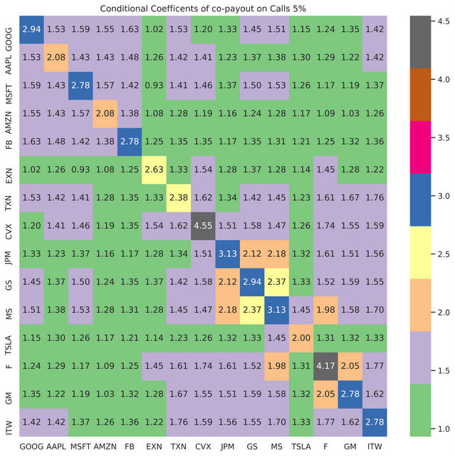
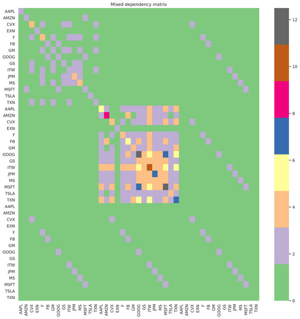
Figure 1. Top: Dependency matrix $5\%$ OTM Call options. Bottom: Dependency matrix $5\%$ and $2\%$ OTM Call, Put and Strangle options.

3.3.2. Properties of $\boldsymbol{\Lambda}$

Positive semi-definiteness

While the dependency matrix $\boldsymbol{\Lambda}$ is symmetric, it may not be positive semi-definite ($\boldsymbol{\mathrm{x}}^{\top}\boldsymbol{\Lambda}\boldsymbol{\mathrm{x}}\geq 0$ for all $\boldsymbol{\mathrm{x}}\in\mathbb{R}^{n}$), as some eigenvalues may be negative. The Perron–Frobenius theorem [32] however ensures that the largest eigenvalue for any irreducible non-negative matrix is greater than zero and all others are bounded by its absolute value. Moreover, from (3.10), Gershgorin’s circle theorem [18] provides bounds for the eigenvalues $\{\lambda_{i}\}_{i=1,\ldots,n}$ of the form $|\lambda_{i}-\Lambda_{ii}|\leq\sum_{j\neq i}\left|\Lambda_{ij}\right|$ for each $i=1,\ldots,n$. In the case where $\boldsymbol{\Lambda}$ is diagonally dominant, namely $|\Lambda_{i}|\geq\sum_{j\neq i}|\Lambda_{ij}|$ for each $i=1,\ldots,n$, then it has positive eigenvalue, and hence is positive semi-definite. While we have found this to hold empirically, there is no guarantee in principle that this will always be true, and we show how to adjust $\boldsymbol{\Lambda}$ to account for this possibility.

Modified Cholesky

If $\boldsymbol{\Lambda}$ is not positive semi-definite, quadratic programming with even a single negative eigenvalue is known to be NP-hard [30], and therefore rather cumbersome from a numerical point of view. We use instead a modified Cholesky algorithm to modify $\boldsymbol{\Lambda}$ slightly to make it positive semi-definite. We consider the set of diagonal matrices $\mathcal{D}$ and following Higham and Cheng [7], for a small constant $\delta\geq 0$, introduce

$$\eta(\boldsymbol{\Lambda},\delta)_{F}:=\min_{\boldsymbol{\mathrm{E}}\in\mathcal{D}}\Big{\{}\|\boldsymbol{\mathrm{E}}\|:\lambda_{\min}(\boldsymbol{\Lambda}+\boldsymbol{\mathrm{E}})\geq\delta\Big{\}},$$

for any matrix norm $\|\cdot\|$. In the particular case of the Frobenius norm, it can be shown that [7, Theorem 3.1]

$$\mu_{F}(\boldsymbol{\Lambda},\delta)=\left(\sum_{\lambda_{i}<\delta}\left(\delta-\lambda_{i}\right)^{2}\right)^{1/2},$$

and the optimal perturbation matrix $\boldsymbol{\mathrm{E}}$ takes the form

(3.11) $$\boldsymbol{\mathrm{E}}=\boldsymbol{Q}\,\mathrm{Diag}(\boldsymbol{\tau})\,\boldsymbol{Q}^{\top},\qquad\text{with}\qquad\tau_{i}:=\left\{\begin{array}[]{ll}0,&\text{if }\lambda_{i}\geq\delta,\\ \delta-\lambda_{i},&\text{if }\lambda_{i}<\delta.\end{array}\right.$$

Remark 3.7.

Note that setting $\delta>0$ from the beginning will return a positive definite modified matrix, which then admits an inverse.

4. Portfolio Optimisation

We now tackle the core of the paper, showing how the dependency matrix becomes a key tool for options portfolio optimisation. For notational clarity, we shall from now on assume that the dependency matrix $\boldsymbol{\Lambda}$ is positive semi-definite, either by construction or after applying the modified Cholesky algorithm from Section 3.3.2.

4.1. Investment procedure

We consider a trader who invests one unit of capital in a portfolio of options every $d$ days. She can buy from a total of $n$ different options, written on $k\leq n$ underlying stocks with a maturity of $d$ trading days, which she then holds to maturity. The options traded in this market include various combinations of Calls, Puts, Strangles and Straddles. If at maturity the options have a positive payout, the trader cashes them in, otherwise she loses all the capital invested in that option. The returns $R_{i}$ on an option $\mathfrak{O}^{i}$ can be characterised as

$$R_{i}:=\frac{\text{Payout}(\mathfrak{O}^{i})-\text{Price}(\mathfrak{O}^{i})}{\text{Price}(\mathfrak{O}^{i})},$$

where $\text{Price}(\mathfrak{O}^{i})$ denotes the price of $\mathfrak{O}^{i}$ at inception of the contract, and the weight of each option $\mathfrak{O}^{i}$ in the portfolio is defined as

$$w_{i}:=\frac{\text{Number of }\mathfrak{O}^{i}\text{ bought}}{\text{Price}(\mathfrak{O}^{i})}.$$

This is of course an ideal setup, as in practice options contracts traded on S$\&$P 500 stocks are traded in multiples of $100$, but this is flexible enough to be updated for practical scenarii. The returns $R^{\pi}$ of the portfolio over the $d$-day period is therefore

$$R^{\pi}=\boldsymbol{\mathrm{w}}^{\top}\boldsymbol{R}=\sum_{i=1}^{n}w_{i}R_{i},$$

where $\boldsymbol{\mathrm{w}}=(w_{1},\ldots,w_{n})$ and $\boldsymbol{R}=(R_{1},\ldots,R_{n})$. Note that this is an ‘all or nothing strategy’ and the trader can potentially lose all her initial capital if none of the options pays out at maturity. This inherent risk in investing in pure option portfolios (especially in deep out-of-the-money options) differs greatly from investing in stocks where it is highly unlikely that all the stocks become worthless.

Remark 4.1.

We only consider portfolios with naked options rather than with options and underlying assets. While this may seem like a risky portfolio (as discussed later), one could construct the corresponding delta-hedged portfolio consisting of assets only, where the amount of each asset is the sum of all the options on this asset, weighted by their deltas.

4.2. Objective function

The goal is to maximise the portfolio returns for a given level of risk. As discussed in the introduction, Markowitz’ portfolio theory uses the returns covariance as a measure of the risk, which is a poor metric here because of the highly asymmetric returns distributions. We consider instead the minimisation problem

$$\min_{\{\boldsymbol{\mathrm{w}}:\boldsymbol{\mathrm{w}}^{\top}\boldsymbol{\mathrm{1}}=1\}}\Big{\{}-\boldsymbol{\mathrm{w}}^{\top}\mathbb{E}[\boldsymbol{R}]+\alpha\boldsymbol{\mathrm{w}}^{\top}\boldsymbol{\Lambda}\boldsymbol{\mathrm{w}}\Big{\}},$$

for some risk aversion parameter $\alpha\geq 0$. The intuition here is that the modified dependency matrix $\boldsymbol{\Lambda}$ has high diagonal terms when option payout probabilities are historically low, which means that weights with low probability of positive payout are penalised. While off-diagonal terms are high if correlation between positive payouts on options are high, thus penalising weights with high correlation of payouts, hopefully leading to a more diverse portfolio. Since the matrix $\boldsymbol{\Lambda}$ is positive semi-definite, the objective function is convex and can be be solved explicitly using Lagrange multipliers. The Lagrangian $\mathcal{L}$ reads

$$\mathcal{L}(\boldsymbol{\mathrm{w}},\gamma):=-\boldsymbol{\mathrm{w}}^{\top}\mathbb{E}[\boldsymbol{R}]+\alpha\boldsymbol{\mathrm{w}}^{\top}\boldsymbol{\Lambda}\boldsymbol{\mathrm{w}}+\gamma\left(\boldsymbol{\mathrm{w}}^{\top}\boldsymbol{\mathrm{1}}-1\right).$$

Equating the gradients $\nabla_{\boldsymbol{\mathrm{w}}}$ and $\partial_{\gamma}$ to zero yields the system

$$\left\{\begin{array}[]{rl}\boldsymbol{\mathrm{0}}&=-\mathbb{E}[\boldsymbol{R}]+2\alpha\boldsymbol{\Lambda}\boldsymbol{\mathrm{w}}+\gamma\boldsymbol{\mathrm{1}},\\ 0&=\boldsymbol{\mathrm{w}}^{\top}\boldsymbol{\mathrm{1}},\end{array}\right.$$

which can be solved explicitly as

(4.1) $$\gamma=\frac{2\alpha-\boldsymbol{\mathrm{1}}^{\top}\boldsymbol{\Lambda}^{-1}\mathbb{E}[\boldsymbol{R}]}{\boldsymbol{\mathrm{1}}^{\top}\boldsymbol{\Lambda}^{-1}\boldsymbol{\mathrm{1}}}\qquad\text{and}\qquad\boldsymbol{\mathrm{w}}=\frac{\boldsymbol{\Lambda}^{-1}}{2\alpha}\left(\mathbb{E}[\boldsymbol{R}]-\boldsymbol{\mathrm{1}}\frac{2\alpha-\boldsymbol{\mathrm{1}}^{\top}\boldsymbol{\Lambda}^{-1}\mathbb{E}[\boldsymbol{R}]}{\boldsymbol{\mathrm{1}}^{\top}\boldsymbol{\Lambda}^{-1}\boldsymbol{\mathrm{1}}}\right).$$

Remark 4.2.

The solution (4.1) assumes that the matrix $\boldsymbol{\Lambda}$ is invertible. The modified Cholesky Algorithm can ensure invertibility setting $\delta>0$, or otherwise we can rely instead on the Moore-Penrose inverse [28, 31].

4.3. Optimisation with box constraints

The framework developed above has several limitations: the quadratic nature of the risk aversion does not distinguish between selling and buying, and hence is not penalising selling options with high probability of payouts. To palliate this issue, we impose short-selling constraints, thus reducing the risk, as the trader is no longer exposed to the unlimited downside created from selling naked options. The trader (because of regulations for example) may also wish to impose diversification constraints, either imposing some non-zero weights or limiting individual amounts; she may also have target proportions of the portfolio in certain categories of assets. The new objective function thus takes the form

(4.2) $$\min_{w_{i}}\left\{\boldsymbol{\mathrm{w}}^{\top}\mathbb{E}[\boldsymbol{R}]-\alpha\boldsymbol{\mathrm{w}}^{\top}\boldsymbol{\Lambda}\boldsymbol{\mathrm{w}}:\boldsymbol{\mathrm{w}}^{T}\boldsymbol{\mathrm{1}}=1,\sum^{m}_{i=1}w_{i}=x,l_{i}\leq w_{i}\leq u_{i}\text{ for }i=1,\ldots,n\right\}$$

Since $\boldsymbol{\Lambda}$ is positive semi-definite, the problem (4.2) is convex quadratic with box constraints. Several classes of algorithms exist to solve such problems, such as Sequential Quadratic Programming [22] or Augmented Lagrangian Methods [2]. We choose the former, a sequential linear-quadratic programming (SLSQP) [35], which is fast and handles well those inequality constraints. We refer the interested reader to [3] for an excellent overview.

5. Results

We now perform out-of-sample back tests over the last four years using a variety of OTM options traded on $15$ S$\&$P 500 stocks, assuming all options are held to maturity. Weights are selected by optimising (4.2) and we also consider different levels of risk aversion $\alpha$ to assess their impact on portfolio performance. Performance is measured using the Sharpe ratio, as well as with moments of the returns distribution. As a comparison, the performance of these portfolios will be benchmarked against an equally weighted portfolio.

5.1. Portfolio construction

We consider two trading scenarios: first on $10\%$ OTM Call options, then on a $5\%$ OTM Call, a $5\%$ OTM Put and a $10\%$ either-side Strangle. All options are bought with one month to maturity and traded on all $15$ S$\&$P 500 stocks, selected from a diverse range of industries. Note that the price of the $10\%$ either side Strangle can be calculated as the sum of $10\%$ OTM Call and Puts. This choice of options and stocks is dictated by liquidity considerations, so that we likely avoid absence of prices for some options on some days. We assume that options can be bought in any quantity, even fractional. While this is not completely true, as options are usually bought in groups, this should not deter the reader from the main message.

We build our trading strategy over $N$ one-month periods $[t_{i},t_{i+1}]$ for $i=0,\ldots,N-1$. At the beginning $t_{i}$ of each period we compute the dependency matrix $\boldsymbol{\Lambda}_{t_{i}}$ (and its modified Cholesky version) with the best of three Archimedean copulas (Frank, Gumbel and Clayton) as well as the expected returns vector $\mathbb{E}_{t_{i}}[\boldsymbol{R}]$, using historic rolling sampling over the past eight years. At time $t_{i}$ we optimise (4.2) with $\boldsymbol{\Lambda}_{t_{i}}$ and $\mathbb{E}_{t_{i}}[\boldsymbol{R}]$ for a selected value of the risk parameter $\alpha$ to obtain the optimal weights $\boldsymbol{\mathrm{w}}_{t_{i}}$. At time $t_{i+1}$, we then compute the returns of the portfolio $R^{\pi}_{t_{i},t_{i+1}}$ over the elapsed period $[t_{i},t_{i+1}]$. The total average returns over the $N$ periods is therefore

$$\overline{R}^{\pi}=\frac{1}{N}\sum_{i=0}^{N-1}R^{\pi}_{t_{i},t_{i+1}},$$

where we assume that we invest the same amount of capital at the start of each period as a normalisation. We evaluate the performance of the portfolio using the Sharpe ratio [25] $\mathrm{SR}:=\frac{1}{\sigma}(\overline{R}^{\pi}-R_{f})$, a standard metric in portfolio management. Here, $\sigma$ represents the standard deviation of returns ($\sigma^{2}=\sum_{i=0}^{N-1}\sigma_{t_{i},t_{i+1}}^{2}$) and where $R_{f}$ is the risk-free rate.

As we have a no short-selling constraint, we are only buying OTM options and are therefore long volatility. We stand to make a lot of money when the market crashes or rises, but in stable markets will steadily lose money. For example, holding a long option portfolio in Spring 2020 would have been hugely profitable as the market crashed and then rebounded. Therefore we expect to see returns with high positive skew and excess kurtosis, with the majority of returns being negative.

5.2. Data

We test the strategy over the period May 2017 to May 2021, requiring samples from May 2009. This period contains a wide variety of market conditions, including highly volatile periods such as the Covid-related market crash in Spring 2020, where the S$\&$P 500 fell over $9.5\%$ on March 12 alone, as well as calmer conditions in 2019 where the VIX averaged at $15.39\%$. On the third Friday of each month we trade one month-to-maturity options on specific S$\&$P 500 stocks (listed below), with expiry on the third Friday of the following month [14]. We automatically exercise the options if they are in the money, using the closing prices from the night before the option expiry date. The only data required for backtest are the opening ask prices of one-month maturity options and their respective stock prices at maturity. The vast majority of S$\&$P 500 options on individual stocks are American and not European. While their prices are slightly higher than their European counterparts, we treat them as holding the contracts to expiry. We only trade on stocks that were listed continuously throughout the sampling and testing periods, excluding for example recently listed stocks (Tesla, Facebook). The $15$ liquidly traded stocks are GOOG, AAPL, MSFT, AMZN, OXY, XOM, HAL, CVX, JPM, GS, MS, JNJ, ABT, F, ITW, distributed between Technology, Financials, Automobiles, Pharmaceuticals and Energy.

5.3. Call option portfolios

We first concentrate on $10\%$ OTM Calls between May 2017 and May 2021. We expect the risk to decrease as we increase the risk aversion parameter $\alpha$, with high dependence being more penalised and weights more evenly distributed between sectors and stocks. To test this we run backtests on $\alpha=0,5,10$, and observe the distributions of weights. We first study the effect of the dependency matrix on the optimal distribution of the weights. When $\alpha=0$, the optimisation problem (4.2) is simply maximising expected returns, without taking into account dependencies between the options. In this case the portfolio consists almost exclusively of Tech stocks as in Figure 2, not surprising since these stocks have performed very well over the last decade. As we increase $\alpha$, the portfolio penalises dependence and diversifies into less dependent Call options, but with high payout probabilities. This is well captured in Figure 2, where $\alpha=10$ creates a more balanced portfolio.

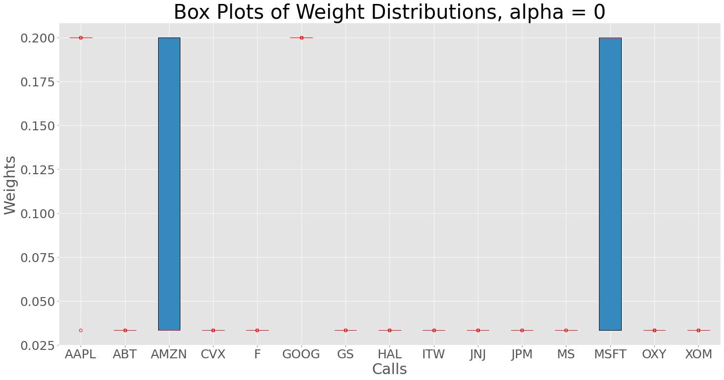
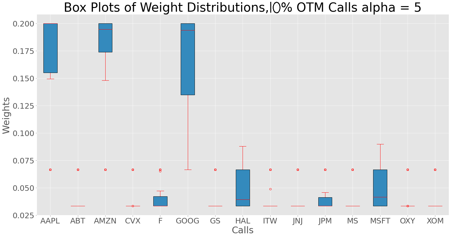
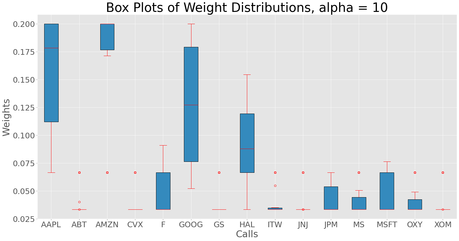
Figure 2. $10\%$ Calls allocation box-plots; $\alpha=0$, $\alpha=5$ and $\alpha=10$.

In Figure 4, we analyse the behaviour of the optimal portfolios over time. At the beginning and the end of the training set, all the weights go to the same value. This occurs since during the $8$-year rolling sampling window, one of the stocks has never seen a $10\%$ or more rise in value in a single month, so that the probability of such an event happening is null, when computed with the empirical cdf. In that case, since some of the denominators in the coefficients  $\Lambda_{ij}$ are null, we set them all to the equally weighted scheme. We leave refinements of this issue to further investigations.

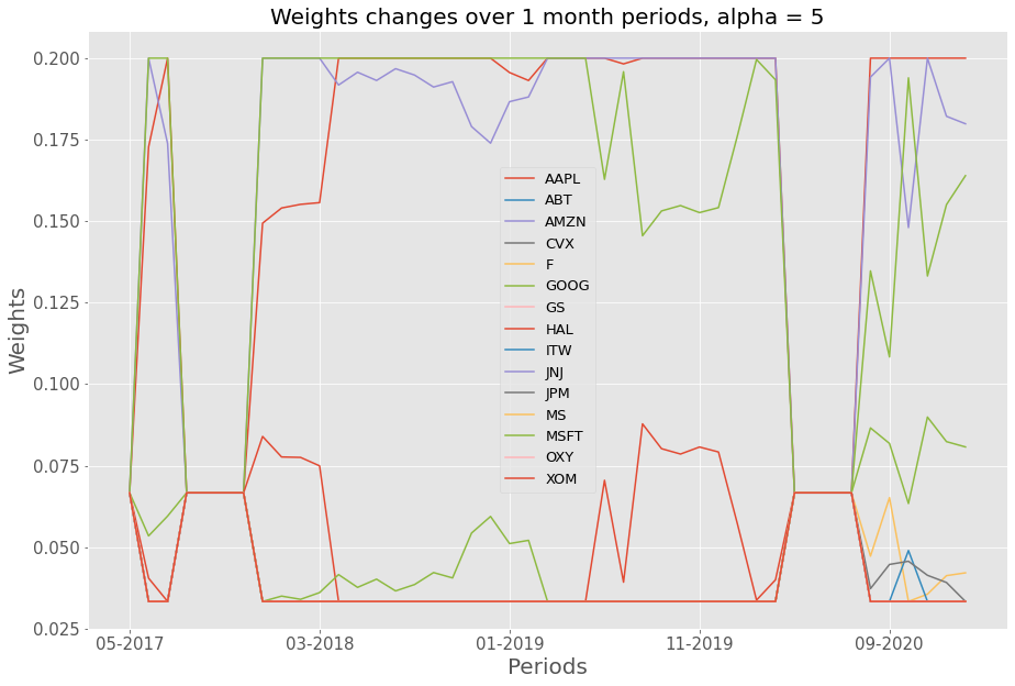
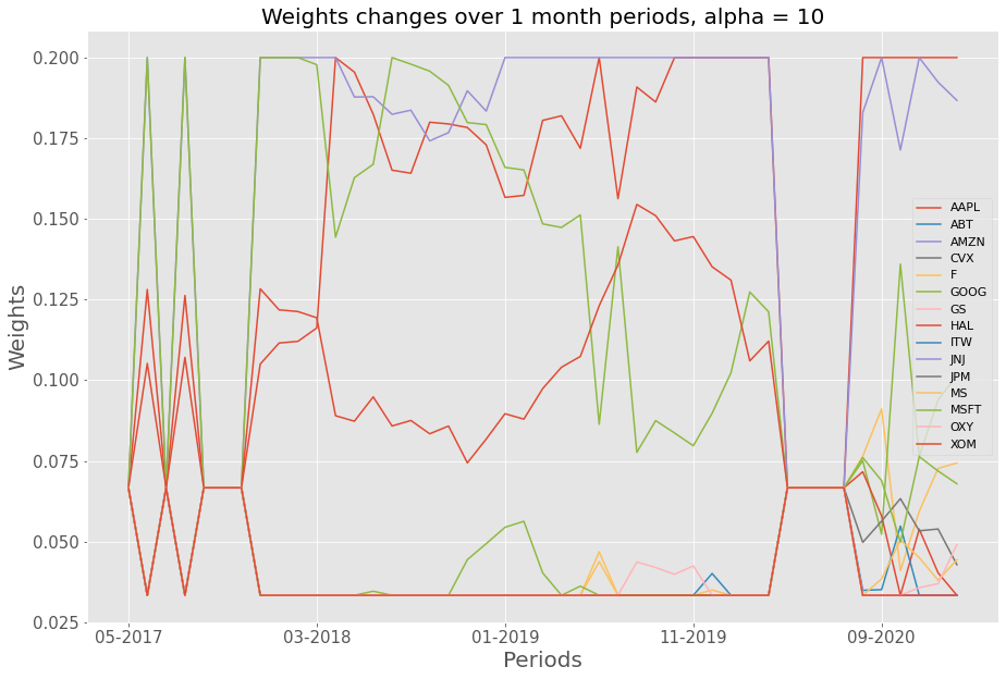
Figure 3. Call portfolio dynamic weight allocation with $\alpha=5$

Figure 4. Call portfolio dynamic weight allocation with $\alpha=10$

We now look at the portfolio performance. Since we only consider one-month $10\%$ OTM Call options, their likelihood of paying out is small. We thus expect to see, even with a very well selected portfolio, many months where returns are equal to $-100\%$. Conversely such deep OTM options are very cheap and thus promise large returns if stocks rise significantly over $10\%$. This would yield returns distribution with positive skew and high kurtosis; this is indeed the case as shown in Figure 5, plotting returns distribution for $\alpha=0$ and $\alpha=10$. The $\alpha=10$ portfolio is less positively skewed than the $\alpha=5$ one, although both are still highly skewed. In comparison, the equally weighted portfolio is clearly less skewed, with lower average returns. The P&L of our portfolios are compared in Figure 6. The $\alpha=0$ portfolio has the highest returns ($85.2\%$), as expected since there is no risk aversion, followed by $\alpha=5$, $\alpha=10$ and finally the equally weighted portfolio. As noted earlier, returns are most often negative and P&L generally trends downwards, except for some occasional months, where large returns push the whole portfolio returns up. This is particularly obvious in Spring 2020, where the optimised portfolio significantly outperformed the equally weighted portfolio, largely due to the large weightings in the over-performing Tech sector. Table 2 summarises the performance of the four portfolios. As expected, the optimal portfolios have high kurtosis and skew, with low Sharpe ratios. The $\alpha=0$ portfolio performs best on Sharpe, but not much more than the other two optimised portfolios. Given the one-month deep OTM Call options considered, the strategy is indeed high risk with low Sharpe ratio.

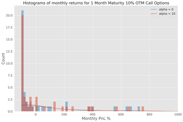
Figure 5. $10\%$ Call options portfolio monthly returns P&L

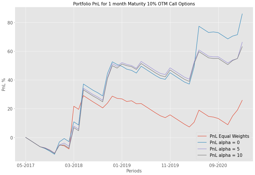
Figure 6. $10\%$ Call options portfolios P&L

	$\alpha=0$	$\alpha=5$	$\alpha=10$	Equal weights
Total return ($\%$)	85.9	66.2	63.1	25.8
Average monthly return ($\%$)	1.87	1.44	1.37	0.56
Kurtosis	32.5	32.8	30.7	14.0
Skew	5.61	5.64	5.4	3.64
Sharpe ratio	0.22	0.20	0.20	0.07

Table 2. $10\%$ Call portfolio Statistics summary.

5.4. Mixed option portfolios

We now test the optimisation on the same stocks using three different options; a $5\%$ OTM Call, $5\%$ OTM Put and a $10\%$ either-side Strangle, all bought with a month to maturity. The optimal weight distribution box-plots for $\alpha\in\{0,5,10\}$ in Figure 7 show that the high-risk $\alpha=0$ strategy favours high-risk options such as the $10\%$ either-side Strangle and ignores Put options. Additionally weights are allocated almost exclusively in the Tech sector and no consideration is made to being overly allocated to the same stocks. For example Amazon is fully allocated in both the Strangle and Call options. This is a very high risk strategy as one relies exclusively on a few stocks. Conversely the $\alpha=10$ portfolio is far more diverse, with a good balance between Calls, Puts and Strangles, allocated between a wide range of sectors. Only Apple is allocated significantly to the Strangle and Call options, which are likely to be highly dependent on each other; other than this outlier, the risk aversion parameter seems to have fulfilled its diversification purpose.

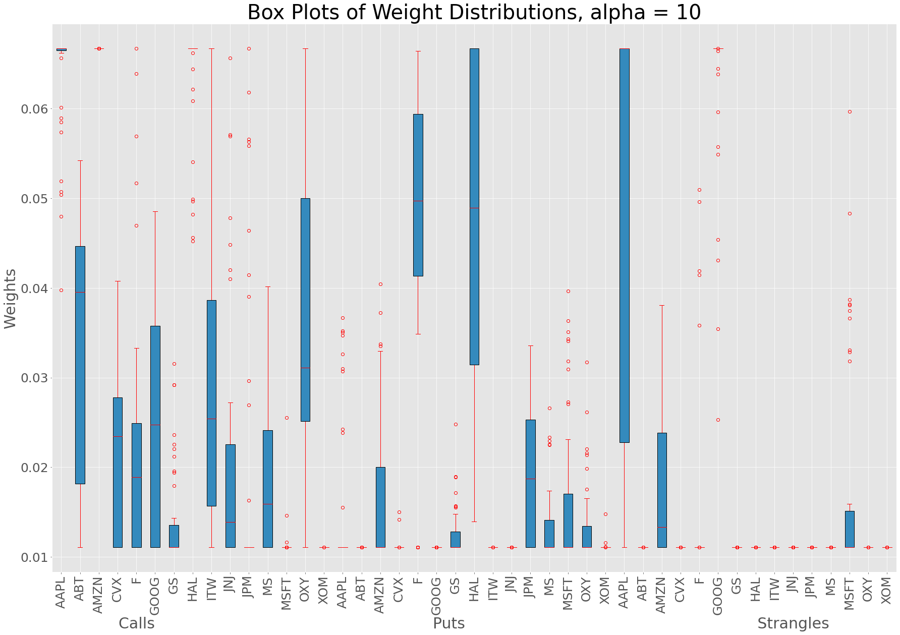
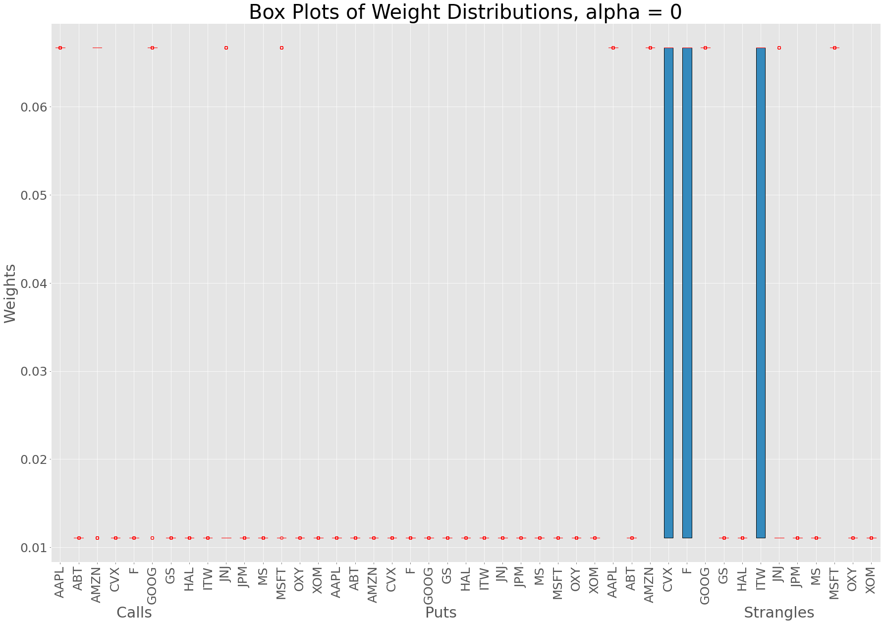
Figure 7. Weight allocation box-plots $\alpha=10$ (left), $\alpha=0$ (right)

The difference in diversity is born out in the returns distributions for the $\alpha=0$ and $\alpha=10$ portfolios, as in Figure 8. There, the $\alpha=10$ portfolio has far fewer $-100\%$ returns. Comparatively the $\alpha=0$ portfolio has far more $-100\%$ months as well as a few very large returns, reflecting the extra risk and associated rewards of maximising the expected returns without penalising dependence. Unsurprisingly $\alpha=0$ demonstrates more skewness than the distribution for $\alpha=10$.

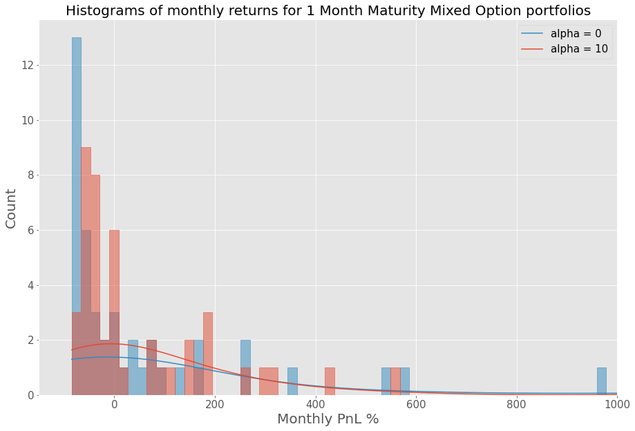
Figure 8. Mixed option portfolios returns distribution.

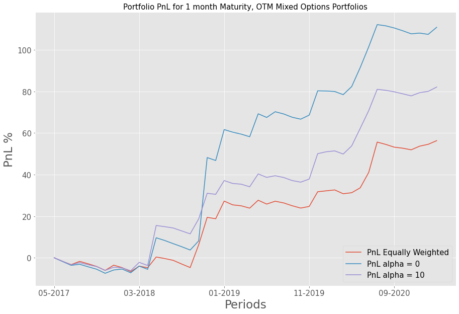
Figure 9. Mixed portfolios P&L.

Figure 9 shows the P&L for the three different strategies. Compared to Figure 6, the trend is smoother as we are trading OTM Puts and Calls closer to the money. The $\alpha=0$ portfolio has the highest return ($111\%$), reliant on large jumps such as during the Covid pandemic, while the $\alpha=10$ portfolio returns only $82.1\%$, with smaller upwards jumps and less steep declines. This is expected from a more diverse portfolio, with less dependence on any one particular stock or sector. Notably, this is what a risk-averse investor would want, showcasing the effectiveness of our dependence penalisation framework. Figure 9 also shows that both our portfolios significantly outperform the equally weighted portfolio. As can be seen in Table 3, the $\alpha=0$ portfolio outperforms the $\alpha=10$ and the equally weighted portfolio in terms of average monthly return. However, it has very high kurtosis and a high positive skew, reflecting the fact that the strategy is very risky, usually losing money before making the occasional large profit. The $\alpha=10$ portfolio has lower average returns, but outperforms both other portfolios in terms of the Sharpe ratio, beating $\alpha=0$ due to the smaller standard deviation in returns. The small Sharpe ratio is again not unexpected since we are trading OTM options. Furthermore, the $\alpha=10$ portfolio’s skew and kurtosis show that it is less reliant on the occasional large returns, as in the $\alpha=0$ case. This supports our approach, reducing the risk by increasing $\alpha$, at the expense of returns.

Mixed options portfolio
Statistic	$\alpha=0$	$\alpha=10$	Equal weights
Total return $\%$	110.9	82.1	56.3
Average monthly return $\%$	2.40	1.78	1.22
Kurtosis	12.8	3.12	2.86
Skew	3.25	1.86	1.88
Sharpe ratio	0.30	0.35	0.26

Table 3. Mixed option portfolio Statistics summary.

Appendix A Additional figures

A.1. Dependency matrices

We provide further empirical examples of dependency matrices $\boldsymbol{\Lambda}$ for different options on S&P 500 stocks, using data from the last eight years. In Figure 10, we show a $10\%$ OTM Put option dependency matrix. The coefficients are extremely high in parts, first as $10\%$ price swings are very rare and second because the sampling period includes an overall bull market for the S&P. The contrast can be seen in Figure 11 with the corresponding Call options, for which the coefficients are much smaller, reflecting that large positive returns were more probable than large negative returns over the period. Figure 12 shows a $5\%$ either-side strangle. The coefficients are lower than in Figures 10 and 11 as we are effectively considering the sum of a Put and Call option, so the probability of payout is higher than for just Calls or Puts. We also clearly see dependence blocks, most significantly around Financials and Automobiles.

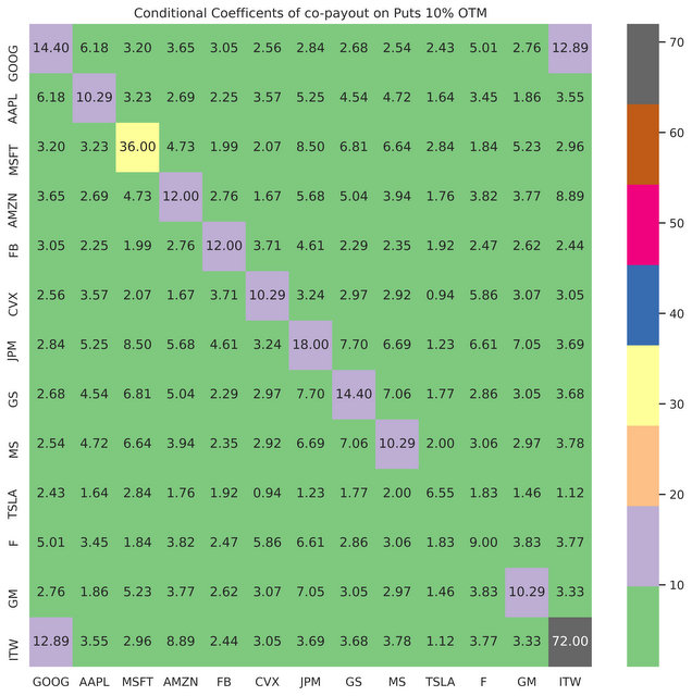
Figure 10. Dependency matrix $10\%$ OTM Put options

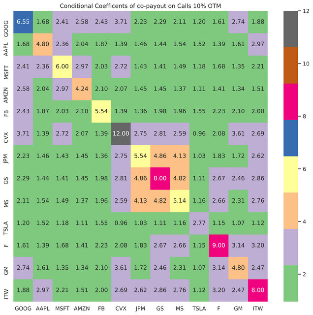
Figure 11. Dependency matrix $10\%$ OTM Call options.

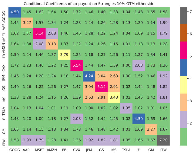
Figure 12. Dependency matrix $10\%$ OTM either-side Strangle options.

A.2. Dynamic weight allocations

Figure 13 shows how weight allocations in the mixed portfolio change for $\alpha=10$ and $\alpha=0$. In the $\alpha=0$ case, where expected returns are maximised without constraints, a few options are exclusively allotted the full allocation and weights barely change at all throughout the period unlike for $\alpha=10$.

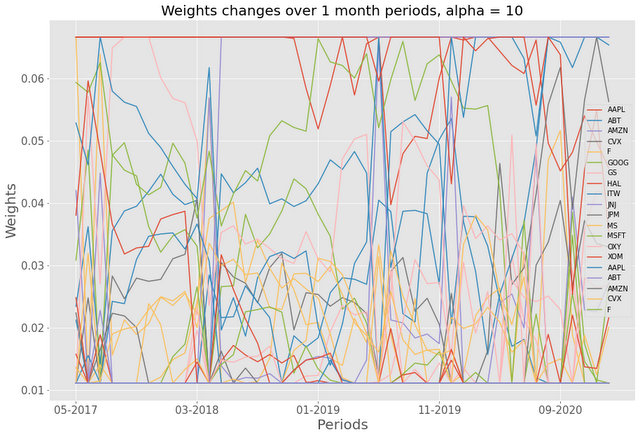
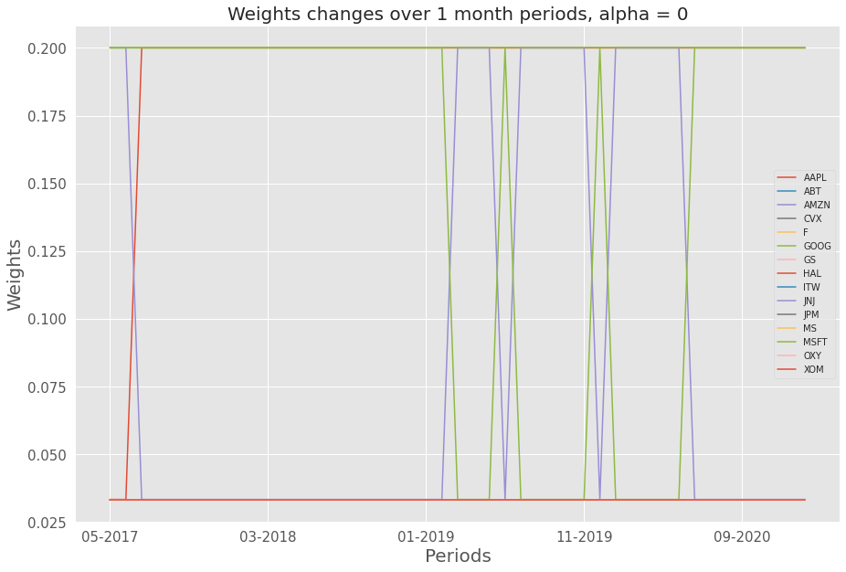
Figure 13. Mixed portfolio dynamic weight allocations with $\alpha=10$ and $\alpha=0$.

References

- [1] R. Ahmad and P. Wilmott, Which free lunch would you like today, sir?: Delta hedging, volatility arbitrage and optimal portfolios, Wilmott, (2005), pp. 64–79.
- [2] E. G. Birgin and J. M. Martínez, Practical augmented Lagrangian methods for constrained optimization, SIAM, 2014.
- [3] P. T. Boggs and J. W. Tolle, Sequential quadratic programming, Acta Numerica, 4 (1995), p. 1–51.
- [4] J.-P. Bouchaud and R. Chicheportiche, The joint distribution of stock returns is not elliptical, International Journal of Theoretical and Applied Finance, 15 (2012), p. 1250019.
- [5] E. C. Brechmann and C. Czado, Risk management with high-dimensional vine copulas: An analysis of the EUROSTOXX 50, Statistics & Risk Modeling, 30 (2013).
- [6] S. Cambanis, S. Huang, and G. Simons, On the theory of elliptically contoured distributions, Journal of Multivariate Analysis, 11 (1981), p. 368–385.
- [7] S. H. Cheng and N. J. Higham, A modified Cholesky algorithm based on a symmetric indefinite factorization, SIAM Journal on Matrix Analysis and Applications, 19 (1998), pp. 1097–1110.
- [8] B. Choroś, R. Ibragimov, and E. Permiakova, Copula estimation, in Copula theory and its applications, Springer, 2010, pp. 77–91.
- [9] J. D. Coval and T. Shumway, Expected option returns, The Journal of Finance, 56 (2001), pp. 983–1009.
- [10] C. Czado, E. Brechmann, and L. Gruber, Selection of vine copulas, Copulae in Mathematical and Quantitative Finance, (2013).
- [11] J. Driessen and P. Maenhout, An empirical portfolio perspective on option pricing anomalies, Review of Finance, 11 (2007), pp. 561–603.
- [12] J. Driessen, P. Maenhout, and G. Vilkov, The price of correlation risk: Evidence from equity options, The Journal of Finance, 64 (2009), pp. 1377–1406.
- [13] B. Eraker, The performance of model based option trading strategies, Review of Derivatives Research, 16 (2013).
- [14] J. Faias and P. Santa-clara, Optimal option portfolio strategies: Deepening the puzzle of index option mispricing, Journal of Financial and Quantitative Analysis, 52 (2017), pp. 277 – 303.
- [15] K. Ferguson and B. Rom, Post-modern portfolio theory comes of age, Journal of Investing, 3 (1994), pp. 11–17.
- [16] J.-D. Fermanian, D. Radulovic, and M. Wegkamp, Weak convergence of empirical copula processes, Bernoulli, 10 (2004), pp. 847 – 860.
- [17] C. Genest, K. Ghoudi, and L.-P. Rivest, A semiparametric estimation procedure of dependence parameters in multivariate families of distributions, Biometrika, 82 (1995), pp. 543–552.
- [18] S. Gerschgorin, Über die abgrenzung der eigenwerte einer matrix, USSR Otd. Fiz.-Mat, (1931), pp. 749–754.
- [19] H. Joe, Families of m-variate distributions with given margins and m(m-1)/2 bivariate dependence parameters., In L. Ruschendorf and B. Schweizer and M. D. Taylor (Ed.), Distributions with Fixed Marginals and Related Topics, (1996).
- [20] H. Joe, Multivariate models and dependence concepts, Monographs on Statistics and Applied Probability, vol. 73 (2001).
- [21] H. Joe, H. Li, and A. K. Nikoloulopoulos, Tail dependence functions and vine copulas, Journal of Multivariate Analysis, 101 (2010), p. 252–270.
- [22] D. Kraft et al., A software package for sequential quadratic programming, (1988).
- [23] B. A. Lengyel and M. H. Stone, Elementary proof of the spectral theorem, Annals of Mathematics, 37 (1936), pp. 853–864.
- [24] D. X. Li, On default correlation, The Journal of Fixed Income, 9 (2000), pp. 43–54.
- [25] A. Lo, The statistics of sharpe ratios, Financial Analysts Journal, 58 (2003).
- [26] S. Malamud, Portfolio selection with options and transaction costs, Swiss Finance Institute Research Paper Series 14-08, 2014.
- [27] H. Markowitz, Portfolio selection, The Journal of Finance, Vol. 7 (1953), pp. 77–91.
- [28] E. Moore, On the reciprocal of the general algebraic matrix, Bull. AMS, 26 (1920), pp. 394–395.
- [29] R. B. Nelsen, An introduction to copulas, Springer Science & Business Media, 2007.
- [30] P. Pardalos and S. Vavasis, Quadratic programming with one negative eigenvalue is NP-hard, Journal of Global Optimisation, 1 (1991), p. 15–22.
- [31] R. Penrose, A generalized inverse for matrices, Proceedings of the Cambridge Philosophical Society, 51 (1955), p. 406–413.
- [32] O. Perron, Zur theorie der matrices, Mathematische Annalen, 64 (1907), pp. 248–263.
- [33] F. Salmon, The formula that killed Wall Street, Significance, 9 (2012), pp. 16–20.
- [34] P. Santa-Clara and A. Saretto, Option strategies: Good deals and margin calls, Journal of Financial Markets, 12 (2009), pp. 391–417.
- [35] K. Schittkowski, The nonlinear programming method of Wilson, Han, and Powell with an augmented lagrangian type line search function. part 2 : An efficient implementation with linear least squares subproblems., Numerische Mathematik, 38 (1982), pp. 115–128.
- [36] A. Sklar, Fonctions de répartition à n dimensions et leurs marges, Publications de l’Institut de Statistique de l’Université de Paris, 8 (1959), p. 229–231.