Unity is strength: improving the detection of adversarial examples with ensemble approaches

Abstract

A key challenge in computer vision and deep learning is the definition of robust strategies for the detection of adversarial examples. Here, we propose the adoption of ensemble approaches to leverage the effectiveness of multiple detectors in exploiting distinct properties of the input data. To this end, the ENsemble Adversarial Detector (ENAD) framework integrates scoring functions from state-of-the-art detectors based on Mahalanobis distance, Local Intrinsic Dimensionality, and One-Class Support Vector Machines, which process the hidden features of deep neural networks. ENAD is designed to ensure high standardization and reproducibility to the computational workflow.

Importantly, extensive tests on benchmark datasets, models and adversarial attacks show that ENAD outperforms all competing methods in the large majority of settings. The improvement over the state-of-the-art and the intrinsic generality of the framework, which allows one to easily extend ENAD to include any set of detectors, set the foundations for the new area of ensemble adversarial detection.

Introduction

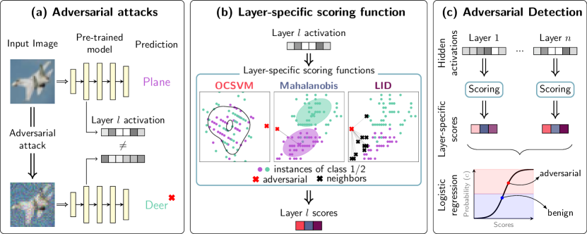
Figure 1: ENAD framework for adversarial detection. A schematic depiction of the ENAD framework is displayed. (a) Given an input image, which can be either benign or adversarial, and a pre-trained deep neural network, the activations of the hidden layers are extracted. (b) In order to measure the distance of the image with respect to training examples, layer-specific scores are computed via functions based either on One-class Support Vector Machines, Mahalanobis distance [26] or Local Intrinsic Dimensionality [31]. (c) Layer- and detector-specific scores are integrated via logistic regression, so to classify the image as benign or adversarial, with a confidence $c$.

Deep Neural Networks (DNNs) have achieved impressive results in complex machine learning tasks, in a variety of fields such as computer vision [24] and computational biology [42].

However, recent studies have shown that state-of-the-art DNNs for object recognition tasks are vulnerable to adversarial examples [45, 11]. For instance, in the field of computer vision, adversarial examples are perturbed images that are misclassified by a given DNN, even if being almost indistinguishable from the original (and correctly classified) image. Adversarial examples have been investigated in many additional real-world applications and settings, including malware detection [22] and speech recognition [38].

Thus, understanding and countering adversarial examples has become a crucial challenge for the widespread adoption of DNNs in safety-critical settings, and resulted in the development of an ever-growing number of defensive techniques. Among the possible countermeasures, some aims at increasing the robustness of the DNN model during the training phase, via adversarial training [45, 11] or defensive distillation [37] (sometimes referred to as proactive methods). Alternative approaches aim at detecting adversarial examples in the test phase, by defining specific functions for their detection and filtering-out (reactive methods).

In this paper, we introduce a novel ensemble approach for the detection of adversarial examples, named ENsemble Adversarial Detector (ENAD), which integrates scoring functions computed from multiple detectors that process the hidden layer activation of pre-trained DNNs. The underlying rationale is that, given the high-dimensionality of the hidden layers of Convolutional Neural Networks (CNNs) and the hardness of the adversarial detection problem, different algorithmic strategies might be effective in capturing and exploiting distinct properties of adversarial examples. Accordingly, their combination might allow one to better tackle the classical trade-off between generalization and overfitting, outperforming single detectors, as already suggested in [3] in the distinct context of outlier identification. To the best of our knowledge, this is the first time that an ensemble approach is applied to the hidden features of DNNs for adversarial detection, while recently a combination of multiple detectors have been proposed for out-of-distribution detection [20].

In detail, ENAD includes two state-of-the-art detectors, based on Mahalanobis distance [26] and Local Intrinsic Dimensionality (LID) [31], and a newly developed detector based on One-Class SVMs (OCSVMs) [41]. OCSVMs were previously adopted for adversarial detection in [30], but we extended the previous method by defining both a pre-processing step and a Bayesian hyperparameter optimization strategy, both of which result fundamental to achieve performances comparable to [31, 26]. In the current implementation, the output of each detector is then integrated via a simple logistic regression that returns both the adversarial classification and the overall confidence of the prediction. A schematic depiction of the ENAD framework is provided in Figure 1.

Importantly, ENAD is designed to ensure a high reproducibility standard of the computational workflow. In fact, similarly to [39], we defined the adversarial detection problem by: (i) clarifying the design choices related to data partitioning and feature extraction, and (ii) explicitly defining the detector-specific scoring functions and the way in which they are integrated. As a consequence, the overall framework of ENAD is completely general and might be easily extended to any arbitrary set of detectors.

For the sake of reproducibility, the performance of ENAD and competing methods was assessed with the extensive setting originally proposed in [26] and, in particular, we performed experiments with two models, namely ResNet [13] and DenseNet [18], trained on CIFAR-10 [23], CIFAR-100 [23] and SVHN [35], and considering four benchmark adversarial attacks, i.e., FGSM [11], BIM [25], DeepFool [34] and CW [5].

Results

We compared the performance of ENAD with stand-alone detectors A (OCSVM), B (Mahalanobis [26]), and C (LID [31]). All four detectors integrate layer-specific anomaly scores via logistic regression and classify any example as adversarial if the posterior probability is $>0.5$, benign otherwise. More details are available in the Methods.

All approaches were tested on $2$ networks architectures (ResNet and DenseNet), $3$ benchmark datasets (CIFAR-10, CIFAR-100 and SVHN) and $4$ adversarial attacks (FGSM, BIM, DeepFool and CW), for a total of $24$ distinct configurations, as originally proposed in [26]. For the evaluation of the performances, we employed two standard threshold-independent metrics, namely the Area Under the Receiver Operating Characteristic (AUROC) and the Area Under Precision Recall (AUPR) [9], which are detailed in the Methods section.

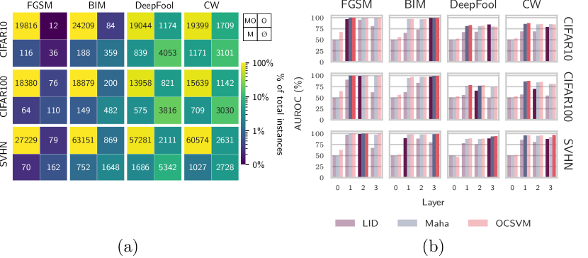
Figure 2: (a) Comparison of predictions of single detectors (OCSVM vs. Mahalanobis – DenseNet). The contingency table shows the number of adversarial examples of the test set $\mathcal{L}^{test}$ correctly identified by: both the OCSVM and the Mahalanobis detectors (OM), either one of the two methods (O or M), none of them ($\emptyset$). The results of the DenseNet model, with respect to the distinct datasets and attacks are shown, whereas the remaining pairwise comparisons are displayed in the Supplementary Material. (b) Influence of the hidden layers in adversarial detection (DenseNet). For each configuration of datasets and attacks on the DenseNet model, the AUROC of each layer-specific score for detectors A–C is returned. For each configuration and detector, the best performing layer is highlighted with a darker shade (see Methods for further details).

Stand-alone Detectors Capture Distinct Properties of Adversarial Examples

In order to assess the ability of detectors A, B and C to exploit different properties of input instances, we first analyzed the methods as stand-alone, and computed the subsets of adversarial examples identified: $(i)$ by all detectors, $(ii)$ by a subset of them, $(iii)$ by none of them.

In Figure 2, we reported a contingency table in which we compare the OCSVM and Mahalanobis detectors on all the experimental settings with the DenseNet model, while the remaining pairwise comparisons are presented in the Supplementary Material. Importantly, while the class of examples identified by both approaches is, as expected, the most crowded, we observe a substantial number of instances that are identified by either one of the two approaches. This important result appear to be general, as it is confirmed in the other comparisons between stand-alone detectors.

In addition, in Supplementary Figure 4 one can find the layer-specific scores returned by all detectors in a specific setting (ResNet, DeepFool, CIFAR-10). For a significant portion of examples, the ranking ordering among scores is not consistent across detectors, confirming the distinct effectiveness in capturing different data properties in the hidden layers.

To investigate the importance of the layers with respect to the distinct attacks, models and datasets, we also computed the AUROC directly on the layer-specific scores, i.e. the anomaly scores returned by each detector in each layer. In Figure 2, one can find the results for all detectors in all settings, with the DenseNet model. For the FGSM attack, the scores computed on the middle layers consistently return the best AUROC in all datasets, while for the BIM attack the last layer is apparently the most important. Notably, with DeepFool and CW attacks the most important layers are dataset-specific. This result demonstrates that each attack may be vulnerable in distinct layers of the network.

ENAD Outperforms Stand-alone Detectors

Table 1 reports the AUROC and AUPR computed on the fitted adversarial posterior probability for detectors A, B, and C, respectively, on all $24$ experimental settings.

It can be noticed that ENAD exhibits both the best AUROC and the best AUPR in $22$ out of $24$ settings (including $1$ tie with OCSVM), with the greatest improvements emerging in the hardest attacks, i.e. DeepFool and CW. Remarkably, the newly designed OCSVM detector outperforms the other stand-alone detectors in 12 and 14 settings in terms of AUROC and AUPR, respectively.

Notice that in Supplementary Table 5, we also evaluated the performance of all pairwise combinations of the three detectors, so to quantitatively investigate the impact of integrating the different algorithmic approaches, proving that distinct ensembles of detectors can be effective in specific experimental settings.

Table 1: Comparative assessment of ENAD and competing methods. Performance comparison of the ENAD, LID [31], Mahalanobis [26], OCSVM detectors (all the pairwise combinations of the three single detectors are available in Supplementary Table 5). The Table contains the AUROC and AUPR for all the combinations of selected datasets (CIFAR-10, CIFAR-100 and SVHN), models (DenseNet and ResNet), and attacks (FGSM, BIM). See Methods for further details.

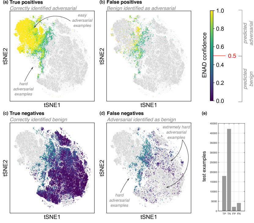
Figure 3: Visualization of adversarial and benign examples in the low-dimensional score space (DenseNet – SVHN – DeepFool). Representation of the test data $\mathcal{L}^{test}$ for the configuration DeepFool, DenseNet and SVHN in the tSNE low-dimensional space [47]. The layer- and detector-specific scores are weighted with the logit weights, Z-scored, and then used as features for the tSNE computation, via the computation of the k-nearest neighbour graph ($k=50$) with Pearson correlation as metric (further tSNE parameters: perplexity = 100, early exaggeration = 100, learning rate = 10000). In each quadrant the true positives (a), false positives (b), true negatives (c) and false negatives (d) are displayed. Each point in the plot represents either an adversarial or a benign example and the color returns the confidence $c$ provided by ENAD, i.e., the probability returned by the logistic classifier. (e) The bar-plots return the absolute number of TPs, TNs, FPs and FNs for this experimental setting.

Visualizing test examples in the low-dimensional score space

In order to explore the relation between the scoring functions and the overall performance of ENAD, it is possible to visualize the test examples on the low-dimensional tSNE space [47], using the (logit weighted and Z-scored) layer- and detector-specific scores as starting features ($3$ detectors $\times$ $4$ hidden layers $=12$ initial dimensions).

This representation allows one to intuitively assess how similar the score profiles of the test examples are: closer data points are those displaying more similar score profiles, which translates in an analogous distance from the set of correctly classified training instances, with respect to the three scoring functions currently included in ENAD. Importantly, this allows one to evaluate how many and which adversarial examples display score profiles closer that those of benign ones, and vice versa, and visualize them.

As an example, in Figure 3 the test set of the SVHN, DenseNet, DeepFool setting is displayed on the tSNE space. The color gradient returns the confidence $c$ of ENAD, i.e., the probability of the logistic regression: any example is categorized as adversarial if $c>0.5$, benign otherwise.

While most of the adversarial examples are identified with high confidence (leftmost region of the tSNE plot), a narrow region exists in which adversarial examples overlap with benign ones, hampering their identification and leading to significant rates of both false positives and false negatives. Focusing on the set of false negatives, it is evident that some adversarial examples are scattered in the midst of the set of benign instances (rightmost region of the tSNE plot), rendering their identification extremely difficult.

ENAD and OCSVM detectors are robust against unknown attacks

We finally assessed the performance of ENAD and detectors A, B, and C when an unknown attack is performed. In detail, we performed the hyperparameters optimization and the logit fit on the FGSM attack, for all methods, and then tested the performance on BIM, DeepFool and CW attacks. Despite the expected worsening of the performances, either ENAD or OCSVM achieve the best AUROC and AUPR in almost all settings (see Table 2), proving their robustness and applicability to the real-world scenarios in which the adversarial example type might be unknown.

Table 2: Comparative assessment in the unknown attack scenario. Performance comparison of the ENAD, LID [31], Mahalanobis [26], and OCSVM detectors when both the hyperparameter optimization and the logistic regression fit are performed on the FGSM attack. The Table contains the AUROC for all the combinations of selected datasets (CIFAR-10, CIFAR-100 and SVHN), models (DenseNet and ResNet), and attacks (BIM, DeepFool and CW). See Methods for further details.

Conclusions

We introduced the ENAD ensemble approach for adversarial detection, motivated by the observation that distinct detectors are able to isolate non-overlapping subsets of adversarial examples, by exploiting different properties of the input data in the internal representation of a DNN. Accordingly, the integration of layer-specific scores extracted from three independent detectors (LID, Mahalanobis and OCSVM) allows ENAD to achieve significantly improved performance on benchmark datasets, models and attacks, with respect to the state-of-the-art, even when the simplest integration scheme (i.e., logit) is adopted.

It is also worth of note that the newly introduced OCSVM detector proved highly effective as stand-alone in our tests, indicating that the use of one-class classifiers for this specific task deserves an in-depth exploration.

Most important, the theoretical framework of ENAD is designed to be completely general, hence it might be extended to include different scoring functions, generated via any arbitrary set of independent algorithmic strategies. In this regard, ongoing efforts aim at integrating detectors processing hidden layer features with others processing the properties of the output, and which have already proven their effectiveness in adversarial detection (see, e.g. [15, 28, 40]). Similarly, one may explore the possibility of exploiting the information on activation paths and/or regions, as suggested in [29, 8], as well as of refining the score definition by focusing on class-conditioned features.

We finally note that the algorithmic framework of ENAD was purposely designed to be as simple as possible, so to unequivocally show the advantages of adopting ensemble approaches in the “cleanest” scenario. However, improvements of the approach are expected to have important implications and should be pursued.

First, the computational time of ENAD is approximately the sum of that of the detectors employed to compute the layer-specific scores and, in the current version, it is mostly affected by OCSVM (see the computation time assessment in Supplementary Figure 2). Efforts should be devoted to tackle the trade-off between effectiveness and scalability, by adopting more efficient implementation schemes and/or constituting detectors.

Second, effective strategies for the integration of the scoring functions might be devised. As shown above, the effectiveness of the detectors and the importance of the layers is closely related to the attack type and, in our case, results in different optimal weights of the logit. As a consequence, in case of unknown attacks, the selection of weights may be complex or even unfeasible, impacting the detector performance. Alternative strategies to combine scores and/or detectors might be considered to improve the generability of our approach, e.g. via weighted averaging or voting schemes [50] or by employing test statistics [39], as well as via the exploitation of more robust feature selection and classification strategies.

Last, adaptive attacks [5], i.e. adversarial example crafted to fool both the classifier and the detector, should be considered to further improve the design of the framework. Even though we expect that the heterogeneous nature of the ensemble would make it difficult to simultaneously fool all constituting detectors, an investigation of score aggregation schemes may be opportune to implement appropriate defense schemes against this kind of attacks.

To conclude, given the virtually limitless possibility of algorithmic extensions of our framework, the superior performance exhibited in benchmark settings in a purposely simple implementation, and the theoretical and application expected impact, we advocate a widespread and timely adoption of ensemble approaches in the field of adversarial detection.

Methods

In this section, we illustrate the ENAD ensemble approach for adversarial detection, as well as the properties of the scoring functions it integrates, respectively based on OCSVM (Detector A - new), Mahalanobis (Detector B) and LID (Detector C), which can also be used as stand-alone detectors. We also describe the background of both adversarial examples generation and detection, the partitioning of the input data and the extraction of the features processed by ENAD and stand-alone detectors.

Background

Notation

Let us consider a multiclass classification problem with $C>2$ classes. Let $\mathcal{N}({\bf\it x})=\sigma_{\text{lgt}}\circ h_{L}\circ\ldots\circ h_{1}({\bf\it x})$ be a DNN with $L$ layers, where $h_{l}$ is the $l^{\text{th}}$ hidden layer and $\sigma_{\text{lgt}}$ is the output layer, i.e. the $C$ logits. To simplify the notation, we refer to the activation of the $l^{\text{th}}$ hidden layer given the input example ${\bf\it x}$, i.e. to $h_{l}\circ\ldots\circ h_{1}({\bf\it x})$, as $h_{l}({\bf\it x})$ and to the logits as $\sigma_{\text{lgt}}({\bf\it x})$. Let $\sigma_{\text{sm}}({\bf\it x})=\sigma_{\text{sm}}(\sigma_{\text{lgt}}({\bf\it x}))$ be the softmax of $\sigma_{\text{lgt}}(x)$, then the predicted class is $\hat{y}=\operatorname*{arg\,max}_{k}\sigma_{\text{sm}}({\bf\it x})^{k}$ with confidence $\hat{p}=\max_{k}\sigma_{\text{sm}}({\bf\it x})^{k}$. Lastly, by $J({\bf\it x},t)=-\log\sigma_{\text{sm}}({\bf\it x})^{t}$ we will denote the cross-entropy loss function given input ${\bf\it x}$ and target class $t$.

Adversarial Attacks Algorithms

In the following, we describe the adversarial attacks that were employed in our experiments, namely FGSM [11], BIM [25], DeepFool [34] and CW [6]:

• FGSM [11] defines optimal $L_{\infty}$ constrained perturbations as:

  $${\bf\it\tilde{x}}={\bf\it x}+\epsilon\cdot\operatorname{sign}{(\gradient_{{\bf\it x}}{J({\bf\it x},t)})},$$

  such that $\epsilon$ is the minimal perturbation in the direction of the gradient that changes the prediction of the model from the true class $y$ to the target class $t$.

• BIM [25] extends FGSM by applying it $k$ times with a fixed step size $\alpha$, while also ensuring that each perturbation remains in the $\epsilon$-neighbourhood of the original image $x$ by using a per-pixel clipping function $\operatorname{clip}$:

  $${\bf\it\tilde{x}_{0}}={\bf\it x}$$

  $${\bf\it\tilde{x}_{n+1}}=\operatorname{clip}_{{\bf\it x},\epsilon}{({\bf\it x_{n}}+\alpha\cdot\operatorname{sign}{(\gradient_{{\bf\it\tilde{x}_{n}}}{J({\bf\it\tilde{x}_{n}},t)})})}$$

• DeepFool [34] iteratively finds the optimal $L_{2}$ perturbations that are sufficient to change the target class by approximating the original non-linear classifier with a linear one. Thanks to the linearization, in the binary classification setting the optimal perturbation corresponds to the distance to the (approximated) separating hyperplane, while in the multiclass the same idea is extended to a one-vs-all scheme. In practice, at each step $i$ the method computes the optimal perturbation $p_{i}$ of the simplified problem, until ${\bf\it\tilde{x}}={\bf\it x}+\sum_{i}p_{i}$ is misclassified.

• the CW $L_{2}$ attack [6] uses gradient descent to minimize $\norm{{\bf\it\tilde{x}}-{\bf\it x}}^{2}+c\cdot l({\bf\it\tilde{x}})$, where the loss $l$ is defined as:

  $$l({\bf\it x})=\max{(\max\{\sigma_{\text{lgt}}({\bf\it\tilde{x}})^{i}:i\neq t\}-\sigma_{\text{lgt}}({\bf\it\tilde{x}})^{t},-\kappa)}.$$

  The objective of the optimization is to minimize the $L_{2}$ norm of the perturbation and to maximize the difference between the target logit $\sigma_{\text{lgt}}({\bf\it\tilde{x}})^{t}$ and the one of the next most likely class up to real valued constant $\kappa$, that models the desired confidence of the crafted adversarial.

Adversarial Detection

Let us consider a classifier $\mathcal{N}$ trained on a training set $\mathcal{X}^{train}$ and a test example ${\bf\it x_{0}}\in\mathcal{X}^{test}$, with predicted label $\hat{y}_{0}$. Adversarial examples detectors can be broadly categorized according to the features they consider: $(i)$ the features of the test example ${\bf\it x_{0}}$, $(ii)$ the hidden features $h_{l}({\bf\it x_{0}})$, or $(iii)$ the features of the output of the network $out({\bf\it x_{0}})$, i.e., the logits $\sigma_{\text{lgt}}({\bf\it x_{0}})$ or the confidence scores $\sigma_{\text{sm}}({\bf\it x_{0}})$.

In brief, the first family of detectors tries to distinguish normal from adversarial examples by focusing on the input data. For instance, in [16] the coefficients of low-ranked principal components of ${\bf\it x_{0}}$ are used as features for the detector. In [12], the authors employed the statistical divergence, such as Maximum Mean Discrepancy, between $\mathcal{X}^{train}$ and $\mathcal{X}^{test}$ to detect the presence of adversarial examples in $\mathcal{X}^{test}$.

The second family of detectors aims at exploiting the information of the hidden features $h_{l}({\bf\it x_{0}})$. In this group, some detectors rely on the identification of the nearest neighbors of $h_{l}({\bf\it x_{0}})$ to detect adversarial examples, by considering either: the conformity of the predicted class among the neighbors [36, 39], the Local Intrinsic Dimensionality [31], the impact of the nearest neighbors on the classifier decision [7] or the prediction of a graph neural-network trained on the nearest neighbors graph [1]. In the same category, additional detectors take into account the conformity of the hidden representation $h_{l}({\bf\it x_{0}})$ to the hidden representation of instances with the same label in the training set, i.e. to $\{h_{l}({\bf\it x_{0}}):\hat{y}_{0}=y,({\bf\it x},y)\in X^{train}\}$, by computing either the Mahalanobis distance [26, 19] to the class means or the likelihoood of a Gaussian Mixture Model (GMM) [49]. Other detectors take the hidden representation $h_{l}({\bf\it x_{0}})$ itself as a discriminating feature, by training either a DNN [33], a Support Vector Machine (SVM) [29], a One-class Support Vector Machine (OSVM) [30] or by using a kernel density estimate [10]. Additional methods within this family use the hidden representation $h_{l}({\bf\it x_{0}})$ as feature to train a predictive model $m_{l}$. The model $m_{l}$ either seeks to predict the same $C$ classes of the original classifier [30, 44] or to reconstruct the input data ${\bf\it x_{0}}$ from $h_{l}({\bf\it x_{0}})$ [16, 15]. The detector then classifies ${\bf\it x_{0}}$ as adversarial/benign by relying on the confidence of the prediction $\hat{y}_{0}$ in the former case, on its reconstruction error in the latter.

The third family of detectors employs the output of the network $out({\bf\it x_{0}})$ to detect adversarial inputs. In this category, some detectors considers the divergence between $out({\bf\it x_{0}})$ and $out(\phi({\bf\it x_{0}}))$ where $\phi$ is a function such as a squeezing function that reduces the features of the input [48], an autoencoder trained on $\mathcal{X}^{train}$ [32], a denoising filter [27] or a random perturbation [40, 17]. Some others take the confidence score of the predicted class $\hat{y}$, that is expected to be lower when the example is anomalous [16, 15, 28]. Lastly, in [10] Bayesian uncertainty of dropout DNNs was used as a feature for the detector.

Data partitioning

Let $\mathcal{X}^{train}$ be the training set on which the classifier $\mathcal{N}$ was trained, $\mathcal{X}^{test}$ the test set and $\mathcal{L}_{norm}\subseteq{\mathcal{X}^{test}}$ the set of correctly classified test instances. Following the setup done in [31, 26], from $\mathcal{L}_{norm}$ we generate $(i)$ a set of noisy examples $\mathcal{L}_{noisy}$ by adding random Gaussian noise, with the additional constraint of being correctly classified, and $(ii)$ a set of adversarial examples $\mathcal{L}_{adv}$ generated via a given attack. We also ensure that $\mathcal{L}_{norm}$, $\mathcal{L}_{noisy}$ and $\mathcal{L}_{adv}$ have the same size. The set $\mathcal{L}=\mathcal{L}_{norm}\cup\mathcal{L}_{noisy}\cup\mathcal{L}_{adv}$ will be our labelled dataset, where the label is $adv$ for adversarial examples and $\overline{adv}$ for benign ones. As detailed in the following sections, $\mathcal{L}$ will be split into a training set $\mathcal{L}^{train}$, a validation set $\mathcal{L}^{valid}$ for hyperparameter tuning and a test set $\mathcal{L}^{test}$ for the final evaluation.

Feature Extraction

In our experimental setting, $h_{l}({\bf\it x})$, with $l\in[1,\dots,L]$, corresponds to either the first convolutional layer or to the output of the $l^{th}$ dense (residual) block of a DNN (e.g. DenseNet or ResNet). As proposed in [26], the size of the feature map is reduced via average pooling, so that $h_{l}({\bf\it x})$ has a number of features equal to the number of channels of the $l^{th}$ layer. Detectors A, B, and C and ENAD are applied to such set of features, as detailed in the following.

Detector A: OCSVM

Algorithm 1 OCSVM detector (see the main text for an explanation of the notation employed)

1:Act. $h_{l}$ of layer $l$, trainset $\mathcal{X}^{train}$, labelled set $\mathcal{L}$

2:for each $l$ in $1,\dots,L$ do

3:     Centering and PCA-whitening of $h_{l}$: $h_{l}^{*}$

4:     Select best layer-specific parameters $\theta=\{\nu,\gamma\}$

5:     Fit OCSVM${}_{l}(\theta)$ on $\{h_{l}^{*}({\bf\it x}):{\bf\it x}\in\mathcal{X}^{train}\}$

6:     OCSVM${}_{l}(\theta)$ decision function: $\text{O}_{l}$

7:     Layer $l$ score of ${\bf\it x_{0}}$: $\text{O}_{l}({\bf\it x_{0}})$

8:end for

9:Scores vector: $\textbf{O}({\bf\it x_{0}}):=[\text{O}_{1}({\bf\it x_{0}}),\dots,\text{O}_{L}({\bf\it x_{0}})]$

10:Fit $adv$ posterior on $\mathcal{L}^{train}$: $p(adv\rvert\textbf{O}({\bf\it x_{0}}))$

11:OCSVM of ${\bf\it x_{0}}$: OCSVM$({\bf\it x_{0}})\coloneqq p(adv\rvert\textbf{O}({\bf\it x_{0}}))$

12:return OCSVM

This newly designed detector is based on a standard anomaly detection technique called One-Class SVM (OCSVM) [41], which belongs to the family of one-class classifiers [46]. One-class classification is a problem in which the classifier aims at learning a good description of the training set and then rejects the inputs that do not resemble the data it was trained on, which represent outliers or anomalies. This kind of classifiers is usually adopted when only one class is sufficiently represented within the training set, while the others are undersampled or hard to be characterized, as in the case of adversarial examples, or anomalies in general. OCSVM was first employed for adversarial detection in [30]. Here, we modified it by defining an input pre-processing step based on PCA-whitening [21], and by employing a Bayesian optimization technique [43] for hyperparameter tuning. The pseudocode is reported in Algorithm 1.

Preprocessing

OCSVM employs a kernel function (in our case a Gaussian RBF kernel) that computes the Euclidean distance among data points. Hence, it might be sound to standardize all the features of the data points, at the preprocessing stage, to make them equally important. To this end, each hidden layer activation $h_{l}({\bf\it x_{0}})$ is first centered on the mean activations $\mu_{l,c}$ of the examples of the training set $\mathcal{X}^{train}$ of class $c$. Then, PCA-whitening $\mathbf{W}^{PCA}_{l}$ is applied:

$$h_{l}^{*}({\bf\it x_{0}}) =\mathbf{W}^{PCA}_{l}\cdot(h_{l}({\bf\it x_{0}})-\mu_{l,c})$$

$$={\bf\it\Lambda}^{-1/2}_{l}\cdot{\bf\it U}^{T}_{l}\cdot(h_{l}({\bf\it x_{0}})-\mu_{l,c}),$$

where ${\bf\it U}^{T}_{l}$ is the eigenmatrix of the covariance $\mathbf{\Sigma}_{l}$ of activations $h_{l}$ and ${\bf\it\Lambda}_{l}$ is the eigenvalues matrix of the examples of $\mathcal{X}^{train}$. Whitening is a commonly used preprocessing technique for outlier detection, since it enhances the separation of points that deviate in low-variance directions [2]. Moreover, in [19] it was conjectured that the effectiveness of the Mahalanobis distance [26] for out-of-distribution and adversarial detection is due to the strong contribution of low-variance directions. Thus, this preprocessing step allows the one-class classifier to achieve better overall performances.

Layer-specific scoring function

After preprocessing, a OCSVM with a Gaussian RBF kernel is trained on the hidden layer activations $h_{l}$ of layer $l$ of the training set $\mathcal{X}^{train}$. Once the model has been fitted, for each instance ${\bf\it x_{0}}$ layer-specific scores $\text{{O}}({\bf\it x_{0}})=[\text{O}_{1}({\bf\it x_{0}}),\text{O}_{2}({\bf\it x_{0}}),\dots,\text{O}_{L}({\bf\it x_{0}})]$ are evaluated. More in detail, let $\mathcal{S}_{l}$ be the set of support vectors, the decision function $\text{O}_{l}({\bf\it x_{0}})$ for the $l^{\text{th}}$ layer is computed as:

$$\text{O}_{l}({\bf\it x_{0}})=\sum_{sv\in\mathcal{S}_{l}}\alpha_{sv}k(h_{l}({\bf\it x_{0}}),sv)-\rho,$$ (1)

where $\alpha_{sv}$ is the coefficient of the support vector $sv$ in the decision function, $\rho$ is the intercept of the decision function and $k$ is a Gaussian RBF kernel with kernel width $\gamma$:

$$k({\bf\it x},{\bf\it y})=\exp(-\gamma\norm{{\bf\it x}-{\bf\it y}}^{2}).$$ (2)

Hyperparameter optimization

The layer-specific scoring function takes two parameters as input: the regularization factor $\nu\in(0,1)$ that controls the fraction of training errors that should be ignored, and the kernel width $\gamma$. This hyperparameters must be carefully chosen to achieve good performances. For this purpose, many approaches have been proposed for hyperparameters selection in OCSVMs [4]. In our setting, we used the validation set of labelled examples $\mathcal{L}^{valid}$ to choose the best combination of parameters, based on the validation accuracy. To avoid a full (and infeasible) exploration of the parameters space, we employed Bayesian hyperparameter optimization, via the scikit-optimize library [14]. In Figure 4, we report the estimated accuracy of the explored solutions in the specific case of the OCSVM detector, in a representative experimental setting.

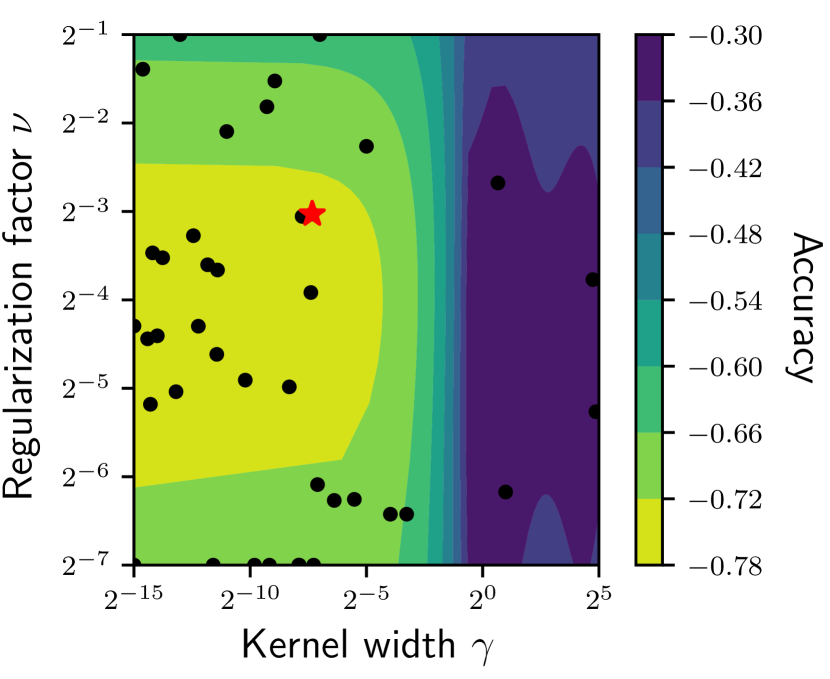
Figure 4: OCSVM hyperparameter optimization. The influence of different combinations of OCSVM hyperparameters $\{\nu,\gamma\}$ on the validation accuracy is explored via Bayesian optimization [14], in the example scenario of DenseNet model, CIFAR-10 dataset and DeepFool attack. The gradient returns the validation accuracy estimated on $\mathcal{L}^{valid}$. The red star represents the optimal configuration, which is then employed for adversarial detection in both the OCSVM and the ENAD detectors.

Adversarial detection

Once the scores have been obtained for each layer, they can serve either as input for the stand-alone detector A or as partial input of the ensemble detector EAD. In the former case, in order to aggregate the scores of the separate layers $\text{{O}}({\bf\it x_{0}})$, this detector employs a logistic regression to model the posterior probability of adversarial ($adv$) examples:

$$\begin{split}&p(adv\rvert\text{{O}}({\bf\it x_{0}}))=\Big{(}1+\exp(\beta_{0}+{\bf\it\beta}^{T}\text{{O}}({\bf\it x_{0}}))\Big{)}^{-1},\\ \end{split}$$ (3)

The parameters $\{\beta_{0},{\bf\it\beta}\}$ are fitted with a cross-validated procedure using the labelled training set $\mathcal{L}^{train}$.

Detector B: Mahalanobis

The Mahalanobis detector was originally introduced in [26]. The algorithmic procedure is akin to that of the OCSVM detector, and includes a final layer score aggregation step via logistic regression, but it is based on a different layer-specific scoring function.

Layer-specific scoring function

Given a test instance ${\bf\it x_{0}}$, the layer score is computed via a three-step procedure: first, for each instance, the class $\hat{c}$ is selected, such that:

$$\hat{c}=\operatorname*{arg\,min}_{c}\text{Maha}_{l}({\bf\it x_{0}},c),$$

where $\text{Maha}_{l}({\bf\it x},c)$ is the Mahalanobis distance for the $l^{\text{th}}$ layer between the activations $h_{l}({\bf\it x})$ and the mean values $\mu_{l,c}$ of the examples in the training set $\mathcal{X}^{train}$:

$$\text{Maha}_{l}({\bf\it x},c)=(h_{l}({\bf\it x})-\mu_{l,c})^{T}{\bf\it\Sigma}_{l}^{-1}(h_{l}({\bf\it x})-\mu_{l,c}),$$ (4)

where ${\bf\it\Sigma}_{l}$ is the covariance matrix of the examples of $\mathcal{X}^{train}$ in layer $l$. Then, the instance is preprocessed to obtain a better separation between benign and adversarial examples similarly to what discussed in [28]:

$${\bf\it x_{0}^{*}}={\bf\it x_{0}}-\lambda\operatorname{sign}{\gradient_{{\bf\it x_{0}}}\text{Maha}_{l}({\bf\it x_{0}},\hat{c})},$$

where $\lambda$ is positive real number, called the perturbation magnitude. The scoring for instance ${\bf\it x_{0}}$ is computed as:

$$\text{{M}}({\bf\it x_{0}})=[\text{M}_{1}({\bf\it x_{0}}),\text{M}_{2}({\bf\it x_{0}}),\dots,\text{M}_{L}({\bf\it x_{0}})],$$

where

$$\text{M}_{l}({\bf\it x_{0}})=-\max_{c}\ {\text{Maha}_{l}({\bf\it x_{0}^{*}},c)}.$$

Adversarial detection

The scores can serve either as input for the stand-alone detector B or as partial input of the ensemble detector EAD. In the latter case, the Mahalanobis detector uses a logistic regression to identify adversarial examples, with a procedure similar to that already described for stand-alone detector A.

Hyperparameter optimization

Differently from detector A, the hyperparameter selection is performed downstream of the adversarial detection stage. In order to select the best $\lambda$ (unique for all layers), the method selects the value that achieves the best Area Under the Receiver Operating Characteristic (AUROC) on $\mathcal{L}^{valid}$ computed on the posterior probability $p(adv\rvert\text{{M}}({\bf\it x_{0}}))$, which is obtained via the logistic regression fitted on $\mathcal{L}^{train}$ (the definition of AUROC is provided in the Supplementary Material).

Detector C: LID

The third detector uses a procedure similar to detectors A-B, but the layer-specific scoring function is based on the Local Intrinsic Dimensionality (LID) approach [31].

Layer-specific scoring function

Given a test instance ${\bf\it x_{0}}$, the LID layer-specific scoring function L is defined as:

$$\text{L}_{l}({\bf\it x_{0}})=-\bigg{(}\frac{1}{k}\sum_{i=1}^{k}\log{\frac{r_{i}(h_{l}({\bf\it x_{0}}))}{\max_{i}r_{i}(h_{l}({\bf\it x_{0}}))}}\bigg{)}^{-1},$$ (5)

where, $k$ is the number of nearest neighbors, $r_{i}$ is the Euclidean distance to the $i$-th nearest neighbor in the set of normal examples $\mathcal{L}_{norm}$. The layer-specific scores are:

$$\text{{L}}({\bf\it x_{0}})=[\text{L}_{1}({\bf\it x_{0}}),\text{L}_{2}({\bf\it x_{0}}),\dots,\text{L}_{L}({\bf\it x_{0}})]$$

Adversarial detection

When considered alone, the LID detector employs a logistic regression to identify adversarial examples, similarly to the other detectors (see above).

Hyperparameter optimization

Similarly to detector B, the hyperparameter selection is performed downstream of the adversarial detection stage. $k$ is selected as the value that achieves the best AUROC on $\mathcal{L}^{valid}$ computed on the posterior probability $p(adv\rvert\text{{L}}({\bf\it x_{0}}))$, which is obtained via the logistic regression fitted on $\mathcal{L}^{train}$. Note that $k$ is unique for all layers.

ENsemble Adversarial Detector (ENAD)

The ENAD approach exploits the effectiveness of detectors A, B, and C in capturing different properties of data distributions, by explicitly integrating the distinct layer-specific scoring functions in a unique classification framework. More in detail, given a test instance ${\bf\it x_{0}}$, it will be characterized by a set of layer-specific and detector-specific features, computed from the scoring functions defined above, that is: $\textbf{E}({\bf\it x_{0}})=[\textbf{O}({\bf\it x_{0}}),\textbf{M}({\bf\it x_{0}}),\textbf{L}({\bf\it x_{0}})]$. It should be noted that training and hyperparameter optimization is executed for each detector independently.

Adversarial detection

In its current implementation, in order to integrate the scores of the separate layers $\textbf{E}({\bf\it x_{0}})$, ENAD employs a simple logistic regression to model the posterior probability of adversarial ($adv$) examples:

$$\begin{split}&p(adv\rvert\textbf{E}({\bf\it x_{0}}))=\Big{(}1+\exp(\beta_{0}+{\bf\it\beta}^{T}\textbf{E}({\bf\it x_{0}}))\Big{)}^{-1}.\\ \end{split}$$ (6)

Like detectors A, B, and C, the logistic is fitted with a cross-validation procedure using the labelled training set $\mathcal{L}^{train}$. Fitting the logistic allows one to have different weights, i.e. the elements of ${\bf\it\beta}^{T}$, for the different layers and detectors, meaning that a given detector might be more effective in isolating an adversarial example when processing its activation on a certain layer of the network. The pseudocode is reported in Algo. 2.

Algorithm 2 ENAD detector.

1:Act. $h_{l}$ of layer $l$, trainset $\mathcal{X}^{train}$, labelled set $\mathcal{L}$

2:Select best hyperparameters for OCSVM, Maha, LID

3:for each layer $l$ in $1,\dots,L$ do

4:     Layer $l$ scores of ${\bf\it x_{0}}$: $\text{O}_{l}({\bf\it x_{0}}),\text{M}_{l}({\bf\it x_{0}}),\text{L}_{l}({\bf\it x_{0}})$

5:end for

6:Scores vector: $\textbf{E}({\bf\it x_{0}})\coloneqq[\textbf{O}({\bf\it x_{0}}),\textbf{M}({\bf\it x_{0}}),\textbf{L}({\bf\it x_{0}})]$

7:Fit $adv$ posterior on $\mathcal{L}^{train}$: $p(adv\rvert\textbf{E}({\bf\it x_{0}}))$

8:ENAD on ${\bf\it x_{0}}$: ENAD$({\bf\it x_{0}})\coloneqq p(adv\rvert\textbf{E}({\bf\it x_{0}}))$

9:return ENAD

Performance Metrics

Let the positive class be the adversarial examples ($adv$) and the negative class be the benign examples ($\overline{adv}$). Then, the correctly classified adversarial and benign examples correspond to the true positives (TP) and true negatives (TN), respectively. Conversely, the wrongly classified adversarial and benign examples are the false negatives (FN) and false positives (FP), respectively.

To evaluate the detectors performances, we employed two standard threshold independent metrics, namely AUROC and AUPR [9], and the accuracy, defined as follows:

• Area Under the Receiver Operating Characteristic curve (AUROC): the area under the curve identified by $\textsf{specificity}=\text{TN}/(\text{TN}+\text{FP})$ and $\textsf{fall-out}=\text{FP}/(\text{FP}+\text{TN})$.

• Area Under the Precision-Recall curve (AUPR): the area under the curve identified by $\textsf{precision}=\text{TP}/(\text{TP}+\text{FP})$ and $\textsf{recall}=\text{TP}/(\text{TP}+\text{FN})$.

• $\textsf{Accuracy}=(\text{TP}+\text{TN})/(\text{TP}+\text{TN}+\text{FP}+\text{FN})$.

The AUROC and AUPR were evaluated given the adversarial posterior learned by the logistic function $p(adv\rvert X)$, were $X$ is the set of layer-specific scores. The layer-specific scores are computed from $\mathcal{L}^{valid}$ when the AUROC is used for hyperparameters optimization for the Mahalanobis and LID detectors, and from $\mathcal{L}^{test}$ in all the other settings, i.e. the detectors performance evaluation. Moreover, AUROC and AUPR were also used to evaluate the performance of each detector in each layer, by consider the layer-specific scores evaluated on $\mathcal{L}^{test}$ (see,. e.g., Figure 2). Note that for the OCSVM and Mahalanobis detectors, lower values corresponds to adversarial examples, while the opposite applies for the LID detector. Finally, the accuracy was used for the Bayesian hyperparameter selection procedure [43] of the OCSVM detector.

References

- [1] Ahmed Abusnaina et al. “Adversarial Example Detection Using Latent Neighborhood Graph” In Proceedings of the IEEE/CVF International Conference on Computer Vision (ICCV), 2021, pp. 7687–7696
- [2] Charu C. Aggarwal “Linear Algebra and Optimization for Machine Learning - A Textbook” New York City: Springer, 2020 DOI: 10.1007/978-3-030-40344-7
- [3] Charu C. Aggarwal and Saket Sathe “Outlier Ensembles - an Introduction” New York City: Springer, 2017 DOI: 10.1007/978-3-319-54765-7
- [4] Shamshe Alam, Sanjay Kumar Sonbhadra, Sonali Agarwal and P. Nagabhushan “One-Class Support Vector Classifiers: A Survey” In Knowl. Based Syst. 196, 2020, pp. 105754 DOI: 10.1016/j.knosys.2020.105754
- [5] Nicholas Carlini and David A. Wagner “Adversarial Examples Are Not Easily Detected: Bypassing Ten Detection Methods” In Proceedings of the 10th ACM Workshop on Artificial Intelligence and Security, AISec@CCS 2017, Dallas, TX, USA, November 3, 2017 Broadway, New York: ACM, 2017, pp. 3–14 DOI: 10.1145/3128572.3140444
- [6] Nicholas Carlini and David A. Wagner “Towards Evaluating the Robustness of Neural Networks” In 2017 IEEE Symposium on Security and Privacy, SP 2017, San Jose, CA, USA, May 22-26, 2017 Washington, D.C., United States: IEEE Computer Society, 2017, pp. 39–57 DOI: 10.1109/SP.2017.49
- [7] Gilad Cohen, Guillermo Sapiro and Raja Giryes “Detecting Adversarial Samples Using Influence Functions and Nearest Neighbors” In 2020 IEEE/CVF Conference on Computer Vision and Pattern Recognition, CVPR 2020, Seattle, WA, USA, June 13-19, 2020 Manhattan, New York, U.S.: IEEE, 2020, pp. 14441–14450 DOI: 10.1109/CVPR42600.2020.01446
- [8] Francesco Craighero et al. “Investigating the Compositional Structure of Deep Neural Networks” In Machine Learning, Optimization, and Data Science Cham: Springer International Publishing, 2020, pp. 322–334
- [9] Jesse Davis and Mark Goadrich “The Relationship between Precision-Recall and ROC Curves” In Machine Learning, Proceedings of the Twenty-Third International Conference (ICML 2006), Pittsburgh, Pennsylvania, USA, June 25-29, 2006 148, ACM International Conference Proceeding Series Pittsburgh, Pennsylvania, USA: ACM, 2006, pp. 233–240 DOI: 10.1145/1143844.1143874
- [10] Reuben Feinman, Ryan R. Curtin, Saurabh Shintre and Andrew B. Gardner “Detecting Adversarial Samples from Artifacts” In CoRR abs/1703.00410, 2017 arXiv:1703.00410
- [11] Ian Goodfellow, Jonathon Shlens and Christian Szegedy “Explaining and Harnessing Adversarial Examples” In International Conference on Learning Representations, 2015
- [12] Kathrin Grosse et al. “On the (Statistical) Detection of Adversarial Examples” In CoRR abs/1702.06280, 2017 arXiv:1702.06280
- [13] Kaiming He, Xiangyu Zhang, Shaoqing Ren and Jian Sun “Deep Residual Learning for Image Recognition” In Proceedings of the IEEE Conference on Computer Vision and Pattern Recognition (CVPR), 2016
- [14] Tim Head et al. “Scikit-Optimize: Sequential Model-Based Optimization in Python” Zenodo DOI: 10.5281/zenodo.1157319
- [15] Dan Hendrycks and Kevin Gimpel “A Baseline for Detecting Misclassified and Out-of-Distribution Examples in Neural Networks” In 5th International Conference on Learning Representations, ICLR 2017, Toulon, France, April 24-26, 2017, Conference Track Proceedings Toulon, France: ICLR, 2017
- [16] Dan Hendrycks and Kevin Gimpel “Early Methods for Detecting Adversarial Images” In 5th International Conference on Learning Representations, ICLR 2017, Toulon, France, April 24-26, 2017, Workshop Track Proceedings Toulon, France: ICLR, 2017
- [17] Bo Huang, Yi Wang and Wei Wang “Model-Agnostic Adversarial Detection by Random Perturbations” In Proceedings of the Twenty-Eighth International Joint Conference on Artificial Intelligence, IJCAI 2019, Macao, China, August 10-16, 2019 Macao, China: IJCAI, 2019, pp. 4689–4696 DOI: 10.24963/ijcai.2019/651
- [18] Gao Huang, Zhuang Liu, Laurens Van Der Maaten and Kilian Q Weinberger “Densely Connected Convolutional Networks” In Proceedings of the IEEE Conference on Computer Vision and Pattern Recognition, 2017, pp. 4700–4708
- [19] Ryo Kamoi and Kei Kobayashi “Why Is the Mahalanobis Distance Effective for Anomaly Detection?” In CoRR abs/2003.00402, 2020 arXiv:2003.00402
- [20] Ramneet Kaur et al. “Detecting OODs as Datapoints with High Uncertainty” In CoRR abs/2108.06380, 2021 arXiv:2108.06380
- [21] Agnan Kessy, Alex Lewin and Korbinian Strimmer “Optimal Whitening and Decorrelation” In The American Statistician 72.4 Taylor & Francis, 2018, pp. 309–314 DOI: 10.1080/00031305.2016.1277159
- [22] Bojan Kolosnjaji et al. “Adversarial Malware Binaries: Evading Deep Learning for Malware Detection in Executables” In 26th European Signal Processing Conference, EUSIPCO 2018, Roma, Italy, September 3-7, 2018 Manhattan, New York, U.S.: IEEE, 2018, pp. 533–537 DOI: 10.23919/EUSIPCO.2018.8553214
- [23] Alex Krizhevsky “Learning Multiple Layers of Features from Tiny Images”, pp. 60
- [24] Alex Krizhevsky, Ilya Sutskever and Geoffrey E. Hinton “ImageNet Classification with Deep Convolutional Neural Networks” In Communications of the ACM 60.6, 2017, pp. 84–90 DOI: 10.1145/3065386
- [25] Alexey Kurakin, Ian J. Goodfellow and Samy Bengio “Adversarial Examples in the Physical World” In 5th International Conference on Learning Representations, ICLR 2017, Toulon, France, April 24-26, 2017, Workshop Track Proceedings Toulon, France: ICLR, 2017
- [26] Kimin Lee, Kibok Lee, Honglak Lee and Jinwoo Shin “A Simple Unified Framework for Detecting Out-of-Distribution Samples and Adversarial Attacks” In Advances in Neural Information Processing Systems 31: Annual Conference on Neural Information Processing Systems 2018, NeurIPS 2018, December 3-8, 2018, Montréal, Canada, 2018, pp. 7167–7177
- [27] Bin Liang et al. “Detecting Adversarial Image Examples in Deep Neural Networks with Adaptive Noise Reduction” In IEEE Trans. Dependable Secur. Comput. 18.1, 2021, pp. 72–85 DOI: 10.1109/TDSC.2018.2874243
- [28] Shiyu Liang, Yixuan Li and R. Srikant “Enhancing the Reliability of Out-of-Distribution Image Detection in Neural Networks” In 6th International Conference on Learning Representations, ICLR 2018, Vancouver, BC, Canada, April 30 - May 3, 2018, Conference Track Proceedings Vancouver, BC, Canada: ICLR, 2018
- [29] Jiajun Lu, Theerasit Issaranon and David A. Forsyth “SafetyNet: Detecting and Rejecting Adversarial Examples Robustly” In IEEE International Conference on Computer Vision, ICCV 2017, Venice, Italy, October 22-29, 2017 Washington, D.C., United States: IEEE Computer Society, 2017, pp. 446–454 DOI: 10.1109/ICCV.2017.56
- [30] Shiqing Ma et al. “NIC: Detecting Adversarial Samples with Neural Network Invariant Checking” In 26th Annual Network and Distributed System Security Symposium, NDSS 2019, San Diego, California, USA, February 24-27, 2019 Reston, Virginia, United States: The Internet Society, 2019
- [31] Xingjun Ma et al. “Characterizing Adversarial Subspaces Using Local Intrinsic Dimensionality” In 6th International Conference on Learning Representations, ICLR 2018, Vancouver, BC, Canada, April 30 - May 3, 2018, Conference Track Proceedings Vancouver, BC, Canada: ICLR, 2018
- [32] Dongyu Meng and Hao Chen “MagNet: A Two-Pronged Defense against Adversarial Examples” In Proceedings of the 2017 ACM SIGSAC Conference on Computer and Communications Security, CCS 2017, Dallas, TX, USA, October 30 - November 03, 2017 Broadway, New York: ACM, 2017, pp. 135–147 DOI: 10.1145/3133956.3134057
- [33] Jan Hendrik Metzen, Tim Genewein, Volker Fischer and Bastian Bischoff “On Detecting Adversarial Perturbations” In 5th International Conference on Learning Representations, ICLR 2017, Toulon, France, April 24-26, 2017, Conference Track Proceedings Toulon, France: ICLR, 2017
- [34] Seyed-Mohsen Moosavi-Dezfooli, Alhussein Fawzi and Pascal Frossard “DeepFool: A Simple and Accurate Method to Fool Deep Neural Networks” In 2016 IEEE Conference on Computer Vision and Pattern Recognition, CVPR 2016, Las Vegas, NV, USA, June 27-30, 2016 Washington, D.C., United States: IEEE Computer Society, 2016, pp. 2574–2582 DOI: 10.1109/CVPR.2016.282
- [35] Yuval Netzer et al. “Reading Digits in Natural Images with Unsupervised Feature Learning” In NIPS Workshop on Deep Learning and Unsupervised Feature Learning 2011, 2011
- [36] Nicolas Papernot and Patrick McDaniel “Deep K-Nearest Neighbors: Towards Confident, Interpretable and Robust Deep Learning” In arXiv:1803.04765 [cs, stat], 2018 arXiv:1803.04765 [cs, stat]
- [37] Nicolas Papernot et al. “Distillation as a Defense to Adversarial Perturbations against Deep Neural Networks” In IEEE Symposium on Security and Privacy, SP 2016, San Jose, CA, USA, May 22-26, 2016 Washington, D.C., United States: IEEE Computer Society, 2016, pp. 582–597 DOI: 10.1109/SP.2016.41
- [38] Yao Qin et al. “Imperceptible, Robust, and Targeted Adversarial Examples for Automatic Speech Recognition” In Proceedings of the 36th International Conference on Machine Learning, ICML 2019, 9-15 June 2019, Long Beach, California, USA 97, Proceedings of Machine Learning Research Long Beach, California, USA: PMLR, 2019, pp. 5231–5240
- [39] Jayaram Raghuram, Varun Chandrasekaran, Somesh Jha and Suman Banerjee “A General Framework for Detecting Anomalous Inputs to DNN Classifiers” In Proceedings of the 38th International Conference on Machine Learning, ICML 2021, 18-24 July 2021, Virtual Event 139, Proceedings of Machine Learning Research Virtual: PMLR, 2021, pp. 8764–8775
- [40] Kevin Roth, Yannic Kilcher and Thomas Hofmann “The Odds Are Odd: A Statistical Test for Detecting Adversarial Examples” In Proceedings of the 36th International Conference on Machine Learning, ICML 2019, 9-15 June 2019, Long Beach, California, USA 97, Proceedings of Machine Learning Research Long Beach, California, USA: PMLR, 2019, pp. 5498–5507
- [41] Bernhard Schölkopf et al. “Support Vector Method for Novelty Detection” In Advances in Neural Information Processing Systems 12, [NIPS Conference, Denver, Colorado, USA, November 29 - December 4, 1999] Cambridge, Massachusetts, United States: The MIT Press, 1999, pp. 582–588
- [42] Andrew W. Senior et al. “Improved Protein Structure Prediction Using Potentials from Deep Learning” In Nat. 577.7792, 2020, pp. 706–710 DOI: 10.1038/s41586-019-1923-7
- [43] Jasper Snoek, Hugo Larochelle and Ryan P. Adams “Practical Bayesian Optimization of Machine Learning Algorithms” In Advances in Neural Information Processing Systems 25: 26th Annual Conference on Neural Information Processing Systems 2012. Proceedings of a Meeting Held December 3-6, 2012, Lake Tahoe, Nevada, United States, 2012, pp. 2960–2968
- [44] Angelo Sotgiu et al. “Deep Neural Rejection against Adversarial Examples” In EURASIP J. Inf. Secur. 2020, 2020, pp. 5 DOI: 10.1186/s13635-020-00105-y
- [45] Christian Szegedy et al. “Intriguing Properties of Neural Networks” In International Conference on Learning Representations Banff, Canada: ICLR, 2014
- [46] DMJ Tax “One-class classification; concept-learning in the absence of counter-examples”, 2001
- [47] Laurens van der Maaten and Geoffrey Hinton “Visualizing Data Using T-SNE” In Journal of Machine Learning Research 9.86, 2008, pp. 2579–2605
- [48] Weilin Xu, David Evans and Yanjun Qi “Feature Squeezing: Detecting Adversarial Examples in Deep Neural Networks” In 25th Annual Network and Distributed System Security Symposium, NDSS 2018, San Diego, California, USA, February 18-21, 2018 Reston, Virginia, United States: The Internet Society, 2018
- [49] Zhihao Zheng and Pengyu Hong “Robust Detection of Adversarial Attacks by Modeling the Intrinsic Properties of Deep Neural Networks” In Advances in Neural Information Processing Systems 31: Annual Conference on Neural Information Processing Systems 2018, NeurIPS 2018, December 3-8, 2018, Montréal, Canada, 2018, pp. 7924–7933
- [50] Zhi-Hua (Computer Zhou “Ensemble Methods : Foundations and Algorithms”, Chapman & Hall/CRC Machine Learning & Pattern Recognition Series Boca Raton: CRC Press, 2012