Supporting Information for
“Stiffening of nanoporous Au as a result of dislocation density increase upon characteristic length reduction"

S.1: Calculation of the characteristic spacing between local centers of the solid or the pore space $\tilde{L}$

A characteristic topological quantity used to characterize the microstructure of NP materials is the spacing between local centers of the solid or the pore space $\tilde{L}$, which can be interpreted as an alternative measure of the mean diameter of the NP Au ligaments ¹. In detail, $\tilde{L}$ can be estimated ^{1, 2} from the topological genus $G$ (i.e., the number of connections in the NP Au microstructure), the scaled genus $g$ (i.e., the number of connections in a representative volume element having size $\tilde{L}^{3}$) and the total volume of the sample $V_{total}$ ² :

$$\tilde{L}=\left(\frac{gV_{total}}{G}\right)^{1/3}$$ (1)

The calculations of $G$ have been performed by estimating, using the CHomP ³ open-source code, the corresponding Betti numbers $B_{0}$ and $B_{1}$, representing a characteristic topological invariant of the NP Au samples. In particular, $B_{0}$ is an estimate of the number of connected components while $B_{1}$ represents the number of handles a the specific structure. The genus is obtained as $G=B_{1}$. The calculation of the scaled genus $g$ have been performed as ²:

$$g=\frac{2\pi\alpha^{3}}{3\sqrt{3}}(1-\xi^{2})e^{-\xi^{2}/2}$$ (2)

where $\alpha$ is the specific surface area and $\xi$ a characteristic function of the volume fraction $\phi$:

$$\xi(\phi)=\sqrt{2}erf^{-1}(2\phi-1)$$ (3)

where $erf$^-1 is the inverse error function.

S.2: Effect of extended defects: grain boundaries

We investigate the effect of grain-boundaries on the Young modulus of single ligaments by positioning in a single gold fcc nanowire (oriented along the (100) direction with length of 20 nm) two grain-boundaries obtained by rotating by an angle $\theta$ the central part (half) of the nanowire with respect to the two top and bottom quarters. Fig. 4 (right) of the main text shows the estimated Young modulus as a function of $D_{nw}$ in the case of different $\theta$ values in the range $0^{\circ}-20^{\circ}$. As opposed to the case of dislocations, the presence of grain-boundaries does not affect the Young modulus for all the $\theta$ values in the range $0^{\circ}-20^{\circ}$.

S.3: Young modulus of a macroscopic gold wire

We theoretically determine the Young modulus of a macroscopic gold wire aligned to the three principal directions (100), (110) and (111) of the cubic crystal. To do this, we assume to apply a stress of the form $\hat{T}=T_{0}\vec{n}\otimes\vec{n}$, where $\vec{n}$ can assume the values (100), (110) or (111) directions. It means that $\hat{T}\vec{m}=0$ if $\vec{m}\perp\vec{n}$, and therefore the lateral surfaces of the wire are supposed to be free. For the cubic structure the stress-strain relation can be summarized as

$$T_{ii} = (C_{11}-C_{12})\varepsilon_{ii}+C_{12}(\varepsilon_{11}+\varepsilon_{22}+\varepsilon_{33}),$$ (4)

$$T_{ij} = 2C_{44}\varepsilon_{ij}\,\,\,(\mbox{if }i\neq j),$$ (5)

where $C_{11}$, $C_{12}$ and $C_{44}$ are the bulk elastic constants. It should be noted that Eqs.4 and 5 reduce to the constitutive relation for an isotropic solid when $2C_{44}=C_{11}-C_{12}$. The embedded-atom model (EAM potential) potential used for the present atomistic simulations predicts $C_{11}$= 78.1 GPa, $C_{12}$= 66.2 GPa and $C_{44}$= 21.2 GPa, in good agreement with experimental data ⁴. By using Eqs. 4 and 5, we determine the strain tensor $\hat{\varepsilon}$, and we evaluate the directional strain $\varepsilon_{0}=\vec{n}\cdot\hat{\varepsilon}\vec{n}$. This allows to calculate the directional Young modulus as $E_{\vec{n}}=T_{0}/\varepsilon_{0}$. The Young modulus for three differently-oriented wires has been eventually obtained in the following form

$$E_{(100)}=\frac{(C_{11}-C_{12})(C_{11}+2C_{12})}{C_{11}+C_{12}},$$ (6)

$$E_{(110)}=\frac{4(C_{11}-C_{12})(C_{11}+2C_{12})C_{44}}{2C_{11}C_{44}+(C_{11}+2C_{12})(C_{11}-C_{12})},$$ (7)

$$E_{(111)}=\frac{3(C_{11}+2C_{12})C_{44}}{2C_{12}+C_{11}+C_{44}}.$$ (8)

The results (dashed lines of Fig. 4 of the main text) represent the asymptotic Young modulus values obtained for macroscopic $D_{nw}$ values for which surface effects becomes less critical.

S.4: Calculation of the local Young modulus

For each atom $i$ of a gold-fcc nanowire containing a single edge-dislocation positioned at z = 6.3 nm, we estimated the the local Young modulus $E^{i}$ by calculating the ratio between the modulus of the per-atom stress tensor $\sigma^{i}$ as implemented in the LAMMPS package ⁵ and the corresponding per-atom elastic strain tensor $\epsilon^{i}$ as implemented in the Ovito package ⁶. Fig. S1 shows a map of the local stress tensor components $\sigma^{i}_{jj}$ (where $jj$= $xx$, $yy$, $zz$) estimated on a nanowire slab having a thickness of 1 nm, while Figure S2 shows a map of the corresponding strain tensor components $\epsilon^{i}_{xx}$, $\epsilon^{i}_{yy}$, $\epsilon^{i}_{zz}$. In both cases we observe a significant $\sigma$ and $\epsilon$ increase in the region (z $<$ 5.5 nm and z $>$ 7.5 nm) where the edge-dislocation was positioned. Figure S3 shows a map of the corresponding local Young modulus (i.e., $\sigma^{i}_{jj}$/$\epsilon^{i}_{jj}$ where $jj$ = $xx$, $yy$ and $zz$) showing a sudden increase up to a value $\sim$ 40 GPa in the region surrounding the dislocation confirming that the presence of dislocations locally increases the elastic properties of the ligaments. Fig. 6 in the main text shows the average value of the local Young modulus over the three $xx$, $yy$ and $zz$ directions.

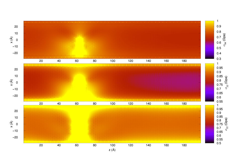
Figure S1: map of the local stress tensor $\sigma^{i}_{jj}$ (where $jj$= $xx$, $yy$, $zz$), calculated on a gold-fcc nanowire (oriented along the (100) direction with D_nw= 3 nm and L_z=20 nm) with a single edge-dislocation positioned at $z$ = 6.3 nm.

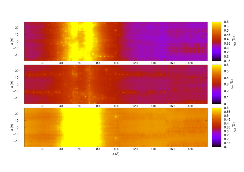
Figure S2: map of the local strain tensor $\epsilon^{i}_{jj}$ (where $jj$= $xx$, $yy$, $zz$), calculated on a gold-fcc nanowire (oriented along the (100) direction with D_nw= 3 nm and L_z=20 nm) with a single edge-dislocation positioned at $z$ = 6.3 nm.

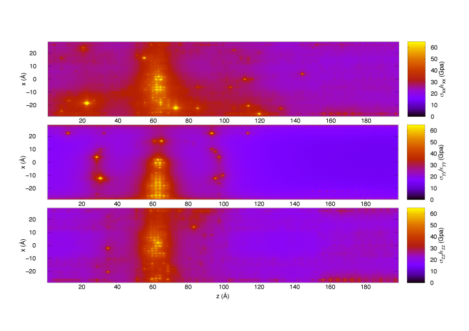
Figure S3: map of the local Young modulus, calculated as the ratio between the local stress and local strain values (i.e., $\sigma^{i}_{jj}$/$\epsilon^{i}_{jj}$ where $jj$ = $xx$, $yy$, $zz$) on a gold-fcc nanowire (oriented along the (100) direction with D_nw= 3 nm and L_z=20 nm) with a single edge-dislocation positioned at $z$ = 6.3 nm.

References

- Li et al. 2019 Li, Y.; Ngô, B.-N. D.; Markmann, J.; Weissmüller, J. Topology evolution during coarsening of nanoscale metal network structures. Physical review materials 2019, 3, 076001
- Soyarslan et al. 2018 Soyarslan, C.; Bargmann, S.; Pradas, M.; Weissmüller, J. 3D stochastic bicontinuous microstructures: Generation, topology and elasticity. Acta materialia 2018, 149, 326–340
- Mischaikow et al. 2014 Mischaikow, K.; Kokubu, H.; Mrozek, M.; Pilarczyk, P.; Gedeon, T.; Lessard, J.-P.; Gameiro, M. Chomp: Computational homology project. Software available at http://chomp. rutgers. edu 2014,
- Neighbours and Alers 1958 Neighbours, J.; Alers, G. Elastic constants of silver and gold. Physical Review 1958, 111, 707
- Plimpton 1995 Plimpton, S. Fast parallel algorithms for short-range molecular dynamics. Journal of computational physics 1995, 117, 1–19
- Stukowski 2009 Stukowski, A. Visualization and analysis of atomistic simulation data with OVITO–the Open Visualization Tool. Modelling and Simulation in Materials Science and Engineering 2009, 18, 015012