Altering Backward Pass Gradients improves Convergence

Abstract

In standard neural network training, the gradients in the backward pass are determined by the forward pass. As a result, the two stages are coupled. This is how most neural networks are trained currently. However, gradient modification in the backward pass has seldom been studied in the literature. In this paper we explore decoupled training, where we alter the gradients in the backward pass. We propose a simple yet powerful method called PowerGrad Transform, that alters the gradients before the weight update in the backward pass and significantly enhances the predictive performance of the neural network. PowerGrad Transform trains the network to arrive at a better optima at convergence. It is computationally extremely efficient, virtually adding no additional cost to either memory or compute, but results in improved final accuracies on both the training and test sets. PowerGrad Transform is easy to integrate into existing training routines, requiring just a few lines of code. PowerGrad Transform accelerates training and makes it possible for the network to better fit the training data. With decoupled training, PowerGrad Transform improves baseline accuracies for ResNet-50 by 0.73%, for SE-ResNet-50 by 0.66% and by more than 1.0% for the non-normalized ResNet-18 network on the ImageNet classification task.

1 Introduction

Backpropagation is traditionally used to train deep neural networks [18]. Gradients are computed using basic calculus principles to adjust the weights during backpropagation [17]. Alternatives to traditional gradients has rarely been studied in the literature hitherto. In normal training procedures, gradients are computed immediately in the backward pass utilizing the values obtained in the forward pass. This makes the backward pass coupled with the forward pass. However, decoupling the backward pass from the forward pass by modifying the gradients to improve training efficiency and final convergent accuracy has hardly been explored. In this paper we explore the landscape of decoupling the forward pass from the backward pass by altering the gradients and subsequently updating the network’s parameters with the modified gradients. There are several ways to achieve gradient modification in the backward pass. We discuss a few techniques in Fig. 1. One could modify the gradients at either (I) multiple points in the backward computation graph or (II) at a point very early in the backward graph and allow this changed gradient to also affect the rest of the network’s gradients as it backpropagates through the backward computation graph.

Figure 1: Different ways of altering gradients in the backward pass. Blue blocks denote a CNN’s different layers (convolutional, linear, batchnorm, softmax, etc.). Orange blocks indicate the backward graph with unmodified gradients. Green blocks represent transformation functions, while red blocks indicate transformed gradients. (a) Type 0: Backpropagation without any gradient modification. (b) Type I: Altering gradients after they are all computed. (c) Type II: Altering gradients at an earlier stage in the backward computation graph, subsequently leading to alteration of all other gradients.

Type 0: No modification: In this method, we calculate the gradients using the standard calculus rules and use the chain rule to calculate the gradients of the rest of the network’s parameters, also known as backpropagation as portrayed in Fig. 1(a). The network is then updated with the gradient descent equation:

$$W_{i}^{t+1}=W_{i}^{t}-\lambda\ \nabla_{W_{i}}(L)\hskip 56.9055pti=D,D-1,\ldots,1$$ (1)

Type I: Gradient modification at multiple points independently: In this method, the gradients are first computed using standard procedure and then individually altered as shown in Fig. 1(b). Gradient clipping [25] and Adaptive gradient clipping [4] are examples of such modifications. In both of these methods, the gradients are first computed using standard rules and then they are modified using some function. It can be described as:

$$W_{i}^{t+1}=W_{i}^{t}-\lambda\ f(\nabla_{W_{i}}(L))\hskip 56.9055pti=D,D-1,\ldots,1$$ (2)

where the gradients $\nabla_{W_{i}}(L)$ are transformed using the transformation function ‘$f$’ before the weight update.

Type II: Gradient modification at a point very early in the backward graph: In this type of modification, the gradient is altered at a very early stage in the backward computation graph and then all subsequent gradients are generated using the values obtained with the modified gradients. We illustrate this type of modification in Fig. 1(c). Because of the chain rule, network parameters whose gradients are connected to the point of alteration in the computation graph also gets subsequently altered. It can be described as:

$$W_{D}^{t+1} =W_{D}^{t}-\lambda\ f(\nabla_{W_{D}}(L))$$ (3)

$$W_{i}^{t+1} =W_{i}^{t}-\lambda\ \nabla_{W_{i}}(L)^{*} i=D-1,\ldots,1$$ (4)

where first the gradient $\nabla_{W_{D}}(L)$ is transformed using the transformation function ‘$f$’ and then this transformed gradient is propagated through the rest of the backward graph. All other gradient vectors $\nabla_{W_{i}}(L)^{*}$ are computed as is, but because of the early injection of the transformed gradient $\nabla_{W_{D}}(L)$, all other gradient vectors that are connected to the transformed gradient through the chain rule ($\nabla_{W_{i}}(L)^{*}$,  i=D-1,…,1), gets subsequently altered.

Type I modification is computationally more expensive than Type II modification as it requires altering the gradients of each and every parameter individually. Type II modification recomputes gradients at each and every location through the natural flow of backpropagation. We propose PowerGrad Transform (PGT) which is a type II gradient modification method. With virtually no additional compute or memory requirement, PowerGrad Transform enhances classification performance of a convolutional neural network, by leading the network to arrive at a higher quality optima at convergence, at which both training and test accuracies improve.

PowerGrad Transform modifies the gradients at the softmax layer, which is the earliest part of most convolutional neural network’s backward computation graph. By changing the gradient at this stage, all other gradients for all other parameters in the network such as the linear layer, batchnorm statistics and convolutional layer’s filter parameters are affected. We analyze and explore the behaviour of such alteration both mathematically and through empirical experiments conducted on networks without batch-normalization. Experimentally, we see that PGT improved training and test accuracies for both normalized and non-normalized networks. PGT improves a network’s learning capacity and results in a better fit of the training data.

The following are the major contributions of this paper:

1. We introduce PowerGrad Transform, which decouples the backward and the forward passes of neural network training and enables a considerably better fit to the dataset, as assessed by both training and test accuracy measures. PGT is a performance enhancement method that alters the gradients in the backward pass before the update step leading to accelerated training and a significant boost in the network’s predictive performance.

2. We perform theoretical analysis of the properties of the PowerGrad transformation (section 4.1) and explore its effect on weight parameters and gradients (section 4.3), logits (section 4.2), (section 5.3), loss values (section 5.3) and class separation (section 4.4).

3. We study experimentally the degenerate behaviour of non-BN networks that is often seen during the normal training procedure, particularly at larger batch sizes. With PGT, we see improved gradient behaviour and a decreased likelihood of the weights attaining degenerate states.

4. We provide complete results from a variety of models (non-BN and BN ResNets, SE-ResNets) using the ImageNet dataset. It helps the network to improve its learning capabilities by locating a more optimum convergence point. Additionally, we conduct an ablation study and compare its impacts to those of regularization approaches such as label smoothing.

2 Related Works

We examine techniques that are related to gradient modification and emphasize the distinction between them and our proposed method.

Gradient Clipping (GC): Gradient Clipping [25], often used in natural language processing methods [22], is a technique that involves changing or clipping the gradients with respect to a predefined threshold value during backward propagation through the network and updating the weights using the clipped gradients [43, 30]. By rescaling the gradients, the weight updates are likewise rescaled, significantly reducing the risk of an overflow or underflow [24]. GC can be used for training networks without batch-normalization.

The formulation is as follows: If $G$ is a gradient vector which is $\partial L/\partial\theta$ (the gradient of the loss $L$ with respect to the parameters $\theta$). In clip by value, the gradients are modified as:

$$G\rightarrow\begin{cases}\lambda\frac{G}{\left\lVert G\right\rVert}&\text{if }\left\lVert G\right\rVert>\lambda,\\ G&\text{otherwise}\end{cases}$$ (5)

At larger batch sizes, the clipping threshold in GC becomes highly sensitive and requires extensive finetuning for various models, batch sizes, and learning rates. As we demonstrate later in our studies, GC is not as effective in improving the performance of non-normalized networks. AGC performs better than GC in non-normalized networks. However, we show that PGT outperforms both in such networks.

Adaptive Gradient Clipping (AGC): Adaptive Gradient Clipping [4] is developed to further enhance backward pass gradients than what is performed by GC. It takes into account the fact that the ratio of the gradient norm to the weight norm can provide an indication of the expected change in a single step of optimization. Here the normalized gradient is clipped by $\lambda$, which means that large weights can have large gradients and still the normalized gradient can be within $\lambda$. If it is not within the threshold, then their gradient is normalized by the ratio of norm of the gradient and norm of the weight in order to avoid gradient explosion. If $W^{l}$ is the weight matrix of the $l^{\textit{th}}$ layer, and $G^{l}$ is its gradient in the backward pass, then the following equation is used to modify the gradient of the $i^{\textit{th}}$ filter before its update:

$$G_{i}^{l}\rightarrow\begin{cases}\lambda\frac{\left\lVert W_{i}^{l}\right\rVert_{F}^{*}}{\left\lVert G_{i}^{l}\right\rVert_{F}}G_{i}^{l}&if\ \frac{\left\lVert G_{i}^{l}\right\rVert_{F}}{\left\lVert W_{i}^{l}\right\rVert_{F}^{*}}\ >\ \lambda\\ G_{i}^{l}&otherwise\end{cases}$$ (6)

The hyperparameter $\lambda$ of AGC is less sensitive to changes in batch size and depth as observed in [4]. However, when applied to vanilla residual networks (ResNet-18), the performance is still afar from normalized variants as demonstrated by our experiments. In most cases, AGC is used for training networks without batch-normalization. Our experiments demonstrate that PGT outperforms AGC, when used independently. When used together, it can further improve a network’s performance (section 5.2).

Label Smoothing: Label smoothing, introduced by Szegedy et al. [31], utilizes smoothing of the ground truth labels as a method to impose regularization on the logits and the weights of the neural network.

The formulation is as follows. If $q_{i}$ is the value at the $i^{th}$ index of the one hot encoded vector of the ground truth label, then the transformed distribution of the labels $q_{i}^{\prime}$ is:

$$q_{i}^{\prime}=\begin{cases}1-\epsilon&\text{if }i=y,\\ \frac{\epsilon}{K-1}&otherwise\end{cases}$$ (7)

where $\epsilon$ is a hyperparameter with a value in $[0,1]$ and $y$ denotes the index of the correct class.

Müller et al. investigates how label smoothing work in [23]. Using visualizations of penultimate layer activations, they demonstrate that label smoothing calibrates the networks predictions and aligns them with the accuracies of the predictions. Parallel works in label smoothing include Pairwise Confusion [8], combatting Label Noise [28], achieving regularization through intentional label modification [37].

PowerGrad Transform works in a much different way. PGT does not smooth the ground truth labels, rather it modifies the gradient by smoothing the predicted probability vector. As we show in section 4, our proposed transformation has the opposite effect of label smoothing. From our studies, we show that PGT in fact leads to larger generalization gap between the training and test dataset, although it does lead to an increase in both training and test accuracies at convergence. Coupled with PGT, label smoothing can narrow the generalization gap, while retaining the benefits of PGT.

Knowledge Distillation: The formulation of PowerGrad Transform is akin to temperature based logit suppression of [15]. Knowledge distillation [3] is a process in which two networks are trained. First a teacher network is trained on a given dataset and then the soft-labels (the predicted probabilities) of the teacher network are used to train another network, called the student network. In similar style of label smoothing, knowledge distillation aims to generate smooth gradient behaviour by forcing the network not to overpredict on any single image. As in case of label smoothing, the student network’s weights are automatically penalized if the network assigns a probability value higher than the soft labels generated by the teacher network. Variants of knowledge distillation include self-distillation [44, 33], identical student network distillation [10], channel distillation [11], regularizing wrong predictions [41] and representation or embedding based knowledge distillation [1, 39, 26]. Distillation is applied to various tasks such as model compression [34], face recognition [12], enhancing ensemble performance [45], interpreting neural networks [20]. Efficacy of distillation is extensivly studied in [5, 40]. Applications of logit suppression include: deep metric learning [42], non-parametric neighborhood component analysis [36], sequence-to-sequence modelling [6], reinforcement learning [14] and face recognition [19, 32].

The key difference between PGT and distillation methods is that in the latter, the transformation is applied in the forward pass, while PGT is a backward pass modification only. Also, in distillation settings the temperature parameter is a part of the network’s computation graph. In the case of PowerGrad Transform, we directly tamper the gradients without introducing any change in the forward pass. It is a more generalized way of arriving at altered gradients in the backward pass. Moreover we show that modifying the gradients in the backward pass can improve performance in many cases. The rise in training accuracy indicates that PGT enables the network to learn more from the training data.

Self-knowledge distillation is used in many papers in different ways, which mainly focuses on improving the performance of the model by either creating multiple ensemble student models [45], using different distorted versions of same data with two different versions of a single network which guides one another [38] or injecting multiple sub-modules in the network to improve its capacity [44]. However none of these methods use normal traditional training without introducing sub-modules in the architecture. PGT differs from self-knowledge distillation as it neither introduces any additional sub-modules nor creates different ensembles to improve the performance of the model. PGT follows the standard neural network training mechanism with a single change which is altering the last layer’s gradients in the backward pass.

Other techniques of weight update include slot machines [2], where random weights are generated and carefully selected during backpropagation in a way that minimizes the loss function.

3 PowerGrad Transform

(a) Unordered distribution

(b) Rank ordered distribution

Figure 2: Illustration of the impact of PowerGrad Transform on probability values of an arbitrary distribution (number of classes, $C=10$). $\alpha=1$ indicates the unmodified distribution. As $\alpha$ reduces from $1$ to $0$, the probability distributions (left: unordered or right: ordered) becomes flatter and flatter, approaching the uniform distribution of $1/C$ for every index.

The PowerGrad Transform technique is described in this section. It is a general technique and can be applied to any neural network. A neural network with parameters $W$ generates $C$ logits denoted by $z$ for every input vector $x$. $z$ is given as $z=Wx$. Then a set of probability values $p_{i}$ are generated from the logits using a softmax function which is defined as $p_{i}=\frac{e^{z_{i}}}{\sum_{j=1}^{C}e^{z_{j}}}$. $p_{i}$ and $z_{i}$ represent the predicted probability values and the logits for the $i^{th}$ class respectively. Following this step, the loss function is invoked and the loss between the predicted probability values the ground truth labels (which is also a probability distribution) is calculated. If the loss function is cross-entropy loss, then the value of the loss is given as $L=-\sum_{i=1}^{C}q_{i}\log\left(p_{i}\right)$ where $q_{i}$ is the ground truth label of the $i^{th}$ class for a particular training example. By standard gradient update rule, we can calculate the gradient of the loss with respect to the logits which takes the form $\frac{\partial L}{\partial z_{i}}=p_{i}-q_{i}$.

The PowerGrad Transform technique is now described. We introduce a hyperparameter $\alpha$, which takes a value between $[0,1]$ and regulates the degree of gradient modification. Fig. 2 shows the effects of the transform under different values of $\alpha$ for different distributions. The PowerGrad Transform method modifies the predicted probability values in the backward pass as follows:

$$\hskip 99.58464ptp_{i}^{\prime}=\frac{p_{i}^{\alpha}}{\sum_{j=1}^{C}p_{j}^{\alpha}}\ \ \ \ \ \ \ \ i=1,\dots,C\ \ \ \ \ 0\leq\alpha\leq 1$$ (8)

The above transformation changes the gradient of the loss with respect to the logits as follows:

$$\widehat{\frac{\partial L}{\partial z_{i}}}=p_{i}^{\prime}-q_{i}$$ (9)

The rest of the backward pass proceeds as usual. We denote the original probability distribution as $P$ (with values $p_{i}$ at the $i^{th}$ index) and the transformed distribution as $P^{\prime}$ (with values $p_{i}^{\prime}$ at the $i^{th}$ index).

A code snippet of the algorithm implemented using PyTorch [27] is given in the appendix. In PyTorch, the available method to modify gradients in the backward pass is using the register_hook function which is called in the forward function. We explore the effect of this change from a theoretical standpoint in section 4. In section 5, we offer empirical data and experiments to support the proposed method.

4 Analysis of the PowerGrad transformation

In this section, we first describe the properties of the PowerGrad Transform (PGT) and then we highlight how these suitable properties of PGT helps the neural network to improve the performance. We use the same setup as described in section 3. To explore the properties of PGT, we start by investigating the effect of the transform on the softmax probabilities.

4.1 Properties of PGT

Lemma 1. For any arbitrary probability distribution $P$ with probability values given by $p_{i}$ for $i=1,\dots,C$, the corresponding transformed probability values $p_{i}^{\prime}$ given by [Eq. 8] has a threshold $\Big{(}\sum_{j=1}^{C}p_{j}^{\alpha}\Big{)}^{\frac{1}{\alpha-1}}$ and

$$\begin{split}p_{i}^{\prime}\geq p_{i}&\text{,\ \ if }p_{i}\leq\Big{(}\sum_{j=1}^{C}p_{j}^{\alpha}\Big{)}^{\frac{1}{\alpha-1}}\\ \hskip 28.45274ptp_{i}^{\prime}<p_{i}&\text{,\ \ if }p_{i}>\Big{(}\sum_{j=1}^{C}p_{j}^{\alpha}\Big{)}^{\frac{1}{\alpha-1}}\end{split}$$ (10)

Proof. The proof follows directly from the definition of $p_{i}^{\prime}$. We notice that if $p_{i}^{\prime}<p_{i}$, we get:

.

$$\ \ \frac{p_{i}^{\alpha}}{\sum_{j=1}^{C}p_{j}^{\alpha}}<p_{i}$$ (11)

$$\Rightarrow \ p_{i}^{\alpha-1}<\sum_{j=1}^{C}p_{j}^{\alpha}$$ (12)

$$\Rightarrow \ p_{i}>\Big{(}\sum_{j=1}^{C}p_{j}^{\alpha}\Big{)}^{\frac{1}{\alpha-1}}$$ (13)

∎

We call this threshold, the stationary threshold. The stationary threshold is that value of $p_{i}$ that does not change after the transformation. Therefore, when $p_{i}$ is greater than the stationary threshold, $p_{i}^{\prime}<p_{i}$.

Proposition 1. At $\alpha=0$, the stationary threshold equals $1/C$ and all values of the transformed distribution $p_{i}^{\prime}$ reduces reduces to the uniform distribution for $i=1,\dots,C$,.

Proof. From Eq. (10), we see that the stationary threshold at $\alpha=0$ is $1/C$. Also, following from the definition of the transformed probabilities (Eq. 8) we conclude that if $\alpha=0$, then all values of $p_{i}^{\prime}$ are $1/C$. Therefore the transformed distribution at $\alpha=0$ is a uniform distribution.

Since we have established that values of $p_{i}$ which are greater than the stationary threshold decreases and move down towards the stationary threshold, and values in $p_{i}$ lower than the stationary threshold moves up towards the stationary threshold, this transformation makes the distribution more uniform (i.e. it smooths out the actual distribution) as $\alpha$ is decreased from $1$ and down towards $0$. This final observation we prove in the following theorem.

Theorem 1. For any arbitrary probability distribution $P$ with probability values $p_{i}$ for $i=1,\dots,C$, the stationary threshold of the transformed distribution $P^{\prime}$ with probability values $p_{i}^{\prime}=\frac{p_{i}^{\alpha}}{\sum_{j=1}^{C}p_{j}^{\alpha}},0\leq\alpha\leq 1$ is a monotonically non-decreasing function with respect to $\alpha$.

Proof. To prove monotonicity, we first compute the gradient of the stationary threshold with respect to the variable in concern, $\alpha$.

$$\frac{\partial}{\partial\alpha}\left(\sum_{j=1}^{c}p_{j}^{\alpha}\right){}^{\frac{1}{\alpha-1}}\ \ =\left(\sum_{j=1}^{c}p_{j}^{\alpha}\right){}^{\frac{1}{\alpha-1}}\left(\frac{\sum_{j=1}^{c}p_{j}^{\alpha}\log\left(p_{j}\right)}{(\alpha-1)\sum_{j=1}^{c}p_{j}^{\alpha}}-\frac{\log\left(\sum_{j=1}^{c}p_{j}^{\alpha}\right)}{(\alpha-1)^{2}}\right)$$ (14)

$$=\frac{1}{\alpha(\alpha-1)^{2}}\left(\sum_{j=1}^{c}p_{j}^{\alpha}\right){}^{\frac{1}{\alpha-1}}\left(\frac{(\alpha-1)\sum_{j=1}^{C}p_{j}^{\alpha}\log\left(p_{j}^{\alpha}\right)}{\sum_{j=1}^{c}p_{j}^{\alpha}}-\alpha\log\left(\sum_{j=1}^{c}p_{j}^{\alpha}\right)\right)$$ (15)

If $a_{1},\dots,a_{n}$ and $b_{1},\dots,b_{n}$ are non-negative numbers, then using the log sum inequality,
we get $\sum_{j=1}^{n}a_{j}\log\left(\frac{a_{j}}{b_{j}}\right)\geq\left(\sum_{j=1}^{n}a_{j}\right)\log\left(\frac{\sum_{j=1}^{n}a_{j}}{\sum_{j=1}^{n}b_{j}}\right)$. Setting $a_{j}=p_{j}^{\alpha}$ and $b_{j}=1$, we get the following lower bound

$$\sum_{j=1}^{C}p_{j}^{\alpha}\log\left(p_{j}^{\alpha}\right)\geq\left(\sum_{j=1}^{C}p_{j}^{\alpha}\right)\log\left(\frac{1}{C}\sum_{j=1}^{C}p_{j}^{\alpha}\right)$$ (16)

Substituting (16) in (15), we get:

$$\frac{\partial}{\partial\alpha}\left(\sum_{j=1}^{c}p_{j}^{\alpha}\right){}^{\frac{1}{\alpha-1}}\ \ \geq\frac{1}{\alpha(\alpha-1)^{2}}\left(\sum_{j=1}^{c}p_{j}^{\alpha}\right){}^{\frac{1}{\alpha-1}}\left((1-\alpha)\log(C)-\log\left(\sum_{j=1}^{C}p_{j}^{\alpha}\right)\right)$$ (17)

$p^{\alpha}$ is concave, and so by Jensen’s inequality we get the following upper bound for the second term:

$$\left(\frac{1}{C}{\sum_{j=1}^{C}p_{j}}{}\right){}^{\alpha}\ \ \geq\ \ \frac{1}{C}{\sum_{j=1}^{C}p_{j}^{\alpha}}{}$$ (18)

$$\Rightarrow\ \ \log\left(\sum_{j=1}^{C}p_{j}^{\alpha}\right)\leq(1-\alpha)\log(C)$$ (19)

Substituting (19) in (17),

.

$$\frac{\partial}{\partial\alpha}\left(\sum_{j=1}^{c}p_{j}^{\alpha}\right){}^{\frac{1}{\alpha-1}}\ \ \geq\ \ 0$$ (20)

∎

We conclude from the analysis that the stationary threshold is a monotonic non-decreasing function with respect to $\alpha$. Also the derivative of PGT function with respect to the true probabilities is non-negative which in turn means that the transformation is an order-preserving map. All values greater than the threshold move towards the threshold after transformation and all values below the threshold also move towards the threshold, and the threshold itself moves monotonically towards $1/C$ as $\alpha$ is decreased from $1$ to $0$. This concludes that the transformation smooths the original distribution.

4.2 PGT restricts the partial derivative of the loss w.r.t. each logit from becoming too small or too high

We know that neural networks uses the softmax function to generate prediction probabilities from logits in multi-class classification tasks. If we use cross-entropy loss to train the network then the partial derivative of the loss w.r.t. $i^{th}$ logit is dependent on the value of the predicted probability and the value of the class label (either 0 or 1) of the $i^{th}$ logit.

$$\frac{\partial L}{\partial z_{i}}=p_{i}-q_{i}$$ (21)

In general, the range of the $|\frac{\partial L}{\partial z_{i}}|$ is [$\delta$, $\epsilon$] where, $\delta\rightarrow 0$ and $\epsilon\rightarrow 1$ in traditional training (Eq. 21 procedures of neural networks. Here, we propose a new method of neural network training which alters the gradients at the time of backward pass by modifying the predicted probability vector using PGT (Eq. 9) such that the directional derivative for each logit does not become too small or too large,

With inclusion of PGT in the last layer, the range of the $\widehat{|\frac{\partial L}{\partial z_{i}}|}$ becomes [$\delta^{+}$, $\epsilon^{-}$] where, $\delta^{+}>\delta$ and $\epsilon^{-}<\epsilon$

Now, we demonstrate how PGT restricts the magnitude of the directional derivative for each logit. For a training example, a neural network can assign the highest probability to either (i) a wrong class or to the (ii) correct class.

(i) Wrong Class Predicted: If the network assigns the highest probability for any class except the the true class, then wrong class assignment happens. We analyze the effect on gradient due to PGT for this case. There are three possibilities

(a) Let, $i^{th}$ class be the class for which the network assigns low probability, but it is the true class, then

$p_{i}<p_{th}\Rightarrow p^{\prime}_{i}>p_{i}\Rightarrow\widehat{\frac{\partial L}{\partial z_{i}}}=p^{\prime}_{i}-1>p_{i}-1$ ; where $p_{i}\rightarrow 0$ & $q_{i}=1$

So; $|\widehat{\frac{\partial L}{\partial z_{i}}}|=|p^{\prime}_{i}-1|<|p_{i}-1|\Rightarrow|\widehat{\frac{\partial L}{\partial z_{i}}}|<\epsilon$ where; $\epsilon\rightarrow 1$

(b) Let, $j^{th}$ class be the class (not true class) for which the network assigns the highest probability, then

$p_{j}>p_{th}\Rightarrow p^{\prime}_{j}<p_{j}\Rightarrow\widehat{\frac{\partial L}{\partial z_{j}}}=p^{\prime}_{j}<p_{j}$ ; where $p_{j}\rightarrow 1$ & $q_{j}=0$

So, $|\widehat{\frac{\partial L}{\partial z_{j}}}|<\epsilon$ where; $\epsilon\rightarrow 1$

(c) Let $k$ denote the index for all those classes for which the predicted probability is low and also the ground truth class label is $0$, then

$p_{k}<p_{th}\Rightarrow p^{\prime}_{k}>p_{k}\Rightarrow\widehat{\frac{\partial L}{\partial z_{k}}}=p^{\prime}_{k}>p_{k}$ ; where $p_{k}\rightarrow 0$ & $q_{k}=0$

So, $|\widehat{\frac{\partial L}{\partial z_{k}}}|>\delta$ where; $\delta\rightarrow$ 0

(ii) Correct Class Predicted: For a given training example, if the network assigns the highest probability to the true class then it assigns correct class to the training example. Now we observe the effect on gradient due to PGT for this case. There are two possibilities,

(a) Let, $i^{th}$ class be the class for which the network assigns the highest probability and it is also the true class, then

$p_{i}>p_{th}\Rightarrow p^{\prime}_{i}<p_{i}\Rightarrow\widehat{\frac{\partial L}{\partial z_{i}}}=p^{\prime}_{i}-1<p_{i}-1$ ; where $p_{i}\rightarrow 1$ & $q_{j}=1$

So; $|\widehat{\frac{\partial L}{\partial z_{i}}}|=|p^{\prime}_{i}-1|>|p_{i}-1|\Rightarrow|\widehat{\frac{\partial L}{\partial z_{i}}}|>\delta$ where; $\delta\rightarrow 0$

(b) Let, $k^{th}$ index is used for all those classes for which the predicted probability is low and also the actual label value $0$, then

$p_{k}<p_{th}\Rightarrow p^{\prime}_{k}>p_{k}\Rightarrow\widehat{\frac{\partial L}{\partial z_{k}}}=p^{\prime}_{k}>p_{k}$ ; where $p_{k}\rightarrow 0$ & $q_{k}=0$

So, $|\widehat{\frac{\partial L}{\partial z_{k}}}|>\delta$ where; $\delta\rightarrow 0$

After analyzing all these cases ((i)a,b,c & (ii)a,b), we are able to deduce that PGT helps to restrict the directional derivative to be within limit such that for every logit/direction the directional derivative is not very small or very large.

4.3 Effect of PGT on weight gradients

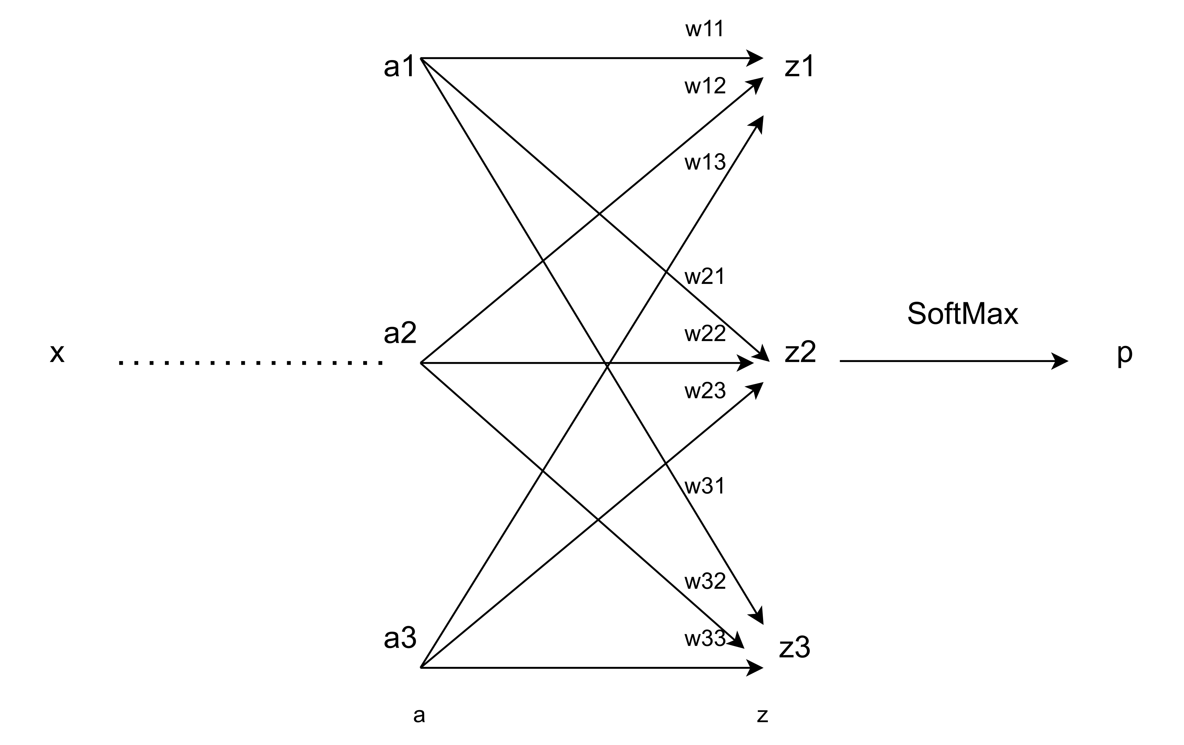
Figure 3: Fully connected layer of a convolutional neural network

In this section, we discuss the impact of PGT on weight gradients. Let the input and output of the last convolutional layer of a convolutional neural network be x and a respectively (Fig. 3). The last layer which is a fully connected layer, produces logits z by combining a with weights and thereafter the network generates the predicted probability vector p from the logits using softmax activation function. We note that a${}_{i}\geq 0$ $\forall i$ as, a is the output of ReLU activation functions.

Here, $z_{i}=\sum_{j=1}^{C}w_{ij}a_{j}$, so $\frac{\partial L}{\partial w_{ij}}=a_{j}\frac{\partial L}{\partial z_{i}}$. However, if we apply PGT while training the neural network, then $\widehat{\frac{\partial L}{\partial w_{ij}}}=a_{j}\widehat{\frac{\partial L}{\partial z_{i}}}$

If the activation of the $j^{th}$ neuron is zero, i.e. $a_{j}=0$ then there is zero gradient for all weights which acts on $a_{j}$ both for normal training and training with PGT, as $a_{j}$ has no contribution in the computation of logits. However, the interesting thing is to observe the effect of PGT when $a_{j}>0$. As, the activation values $(a_{j})$ are positive, so $\widehat{\frac{\partial L}{\partial z_{i}}}>\frac{\partial L}{\partial z_{i}}\Rightarrow$ $\widehat{\frac{\partial L}{\partial w_{ij}}}>\frac{\partial L}{\partial w_{ij}}\forall j\in(1,2,\ldots C)$ and similar relationship for $a_{j}<0$. With PGT, the weight updating rule for $(t+1)^{th}$ iteration then becomes,

$$w_{ij}^{t+1}=w_{ij}^{t}-\eta\widehat{\frac{\partial L}{\partial w_{ij}^{t}}}$$ (22)

The weight update equation using PGT, can also be viewed in terms of the following equation,

$$w_{ij}^{t+1}=w_{ij}^{t}-\frac{\eta}{C_{PGT}}\frac{\partial L}{\partial w_{ij}^{t}}$$ (23)

For neural networks, the exponential nature of the softmax function produces sharp distribution for predicted probability vector. For example, if z is $[20,30,10]$ then p is equal to $[4\times 10^{-5},0.99995,2\times 10^{-9}]$. When the network is at the initial phase of training, most of the training examples are misclassified. Under this scenario, PGT helps to update the weights in a better manner than traditional gradients. Suppose the label vector q is $[1,0,0]$ then it indicates that $z_{1}$ is the logit corresponding to ground truth class and $z_{2}$ is the logit where the network has assigned the highest probability. Similarly, $z_{3}$ is the logit where the network has assigned a low probability as well as the label vector is also $0$ for this logit. Here $\frac{\partial L}{\partial w_{1j}^{t}}=\epsilon a_{j}>0\Rightarrow$ $\widehat{\frac{\partial L}{\partial w_{1j}^{t}}}<\frac{\partial L}{\partial w_{1j}^{t}}\Rightarrow C_{PGT}>1$ $\forall j\in(1,2,\ldots C)$. Advanced gradient updation algorithms like AdaGrad [9] reduces the gradient in the direction where the directional derivative for a weight is high. It reduces the learning rate for the weight so that the gradient in that direction is not too large in order to make the update process less volatile. The formulation of PGT also implicitly reduces the partial derivative in the same manner for the high derivative directions, the only difference with the AdaGrad is that $C_{PGT}$ depends only on the current iteration’s gradient and not on previous iterations like AdaGrad. Similarly we can observe that for this example, $\frac{\partial L}{\partial w_{3j}^{t}}=\delta a_{j}\approx 0\Rightarrow$ $\widehat{\frac{\partial L}{\partial w_{3j}^{t}}}>\frac{\partial L}{\partial w_{3j}^{t}}\Rightarrow C_{PGT}<1$ $\forall j\in(1,2,\ldots C)$. As directional derivative for the weights associated with third logit is extremely low, PGT helps to increase the derivative in these directions so that the training process does not become too slow.

4.4 Effect of PGT on class separation

During final iterations of training, we analyze the iteration-wise gradient behaviour where the network assigns the highest probability to the correct class for a given training example; we deduce the effects of PGT in the next immediate training iteration. For example, if z is $[30,20,10]$ then p is $[0.99995,4\times 10^{-5},2\times 10^{-9}]$ and q is $[1,0,0]$. There is no change in the weight update due to PGT when $a_{j}=0$. However, when $i\neq 1$ and $a_{j}>0$, $|\widehat{\frac{\partial L}{\partial w_{1j}^{t}}}|>|\frac{\partial L}{\partial w_{1j}^{t}}|$ and $\widehat{\frac{\partial L}{\partial w_{ij}^{t}}}>\frac{\partial L}{\partial w_{ij}^{t}}$. Here in this example $\frac{\partial L}{\partial z_{1}^{t}}<0\Rightarrow\frac{\partial L}{\partial w_{1j}^{t}}<0\Rightarrow$ $\widehat{w_{1j}^{t+1}}>w_{1j}^{t+1}>w_{1j}^{t}\forall j$. We also know that $z_{i}^{t+1}=\sum_{j=1}^{C}w_{ij}^{t+1}a_{j}$ and $\widehat{z_{i}^{t+1}}=\sum_{j=1}^{C}\widehat{w_{ij}^{t+1}}a_{j}$. It indicates that $\widehat{z_{1}^{t+1}}>z_{1}^{t+1}>z_{1}^{t}$ as all the weights associated with first logit is larger while using PGT in $(t+1)^{th}$ iteration. Similarly, for the non-true classes $\widehat{w_{ij}^{t+1}}<w_{ij}^{t+1}<w_{ij}^{t}$ when $i\neq 1$ $\forall j$ as $\frac{\partial L}{\partial z_{i}^{t}}>0$. So in $(t+1)^{th}$ iteration, $\widehat{z_{i}^{t+1}}<z_{i}^{t+1}<z_{i}^{t}$ when $i\neq 1$. We observe that $dist(\widehat{z_{1}^{t+1}},\widehat{z_{i}^{t+1}})>$ $dist(z_{1}^{t+1},z_{i}^{t+1})$ where the first logit corresponds to the true class and all other logits indexed by $i$ are non-true classes. Therefore the distance between correct and incorrect class logits increases due to PGT and this leads to better class separation.

5 Experiments

5.1 Experiments on convolutional neural networks (with batch-normalization)

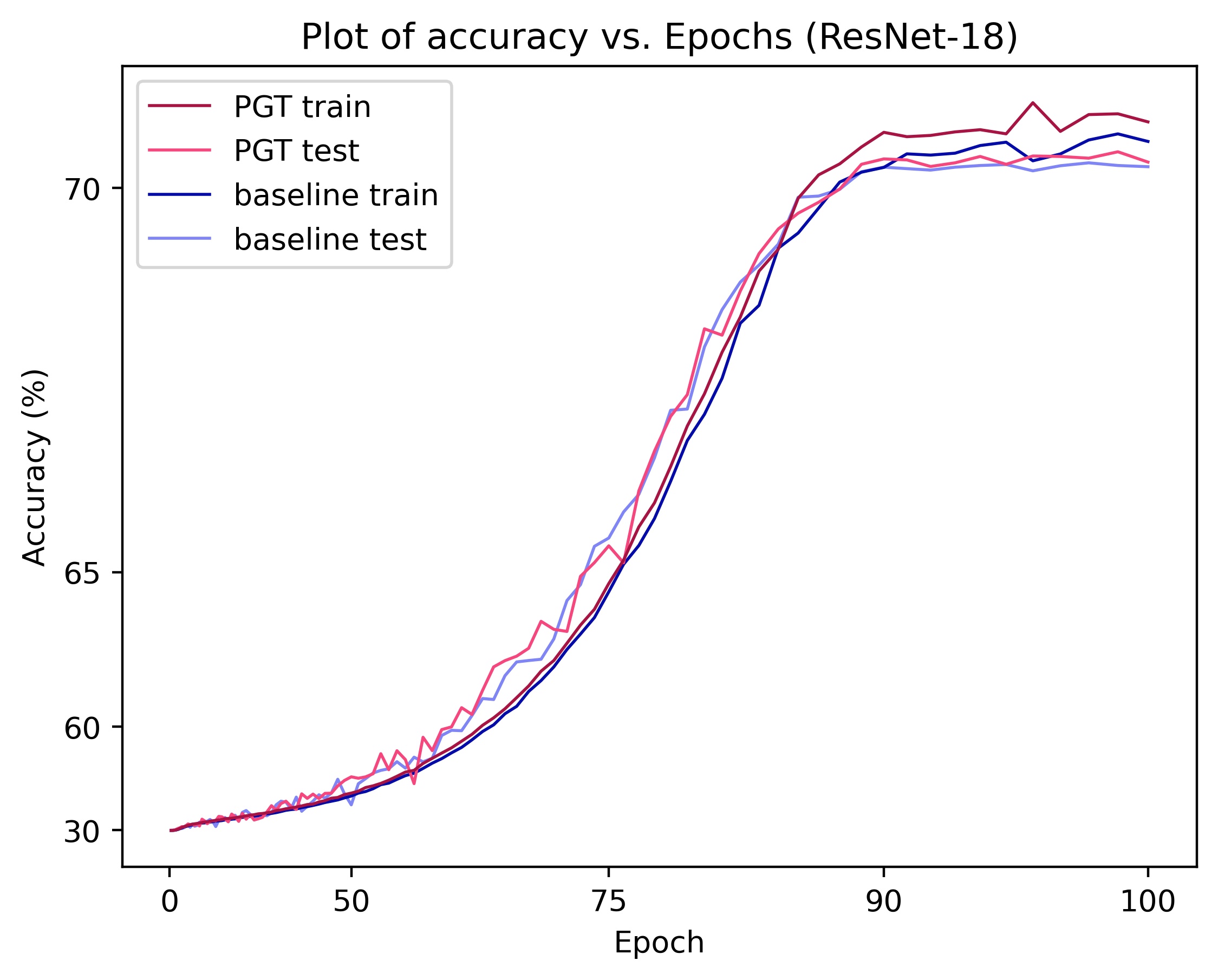
(a) Plot of training and test accuracies (ResNet-18)

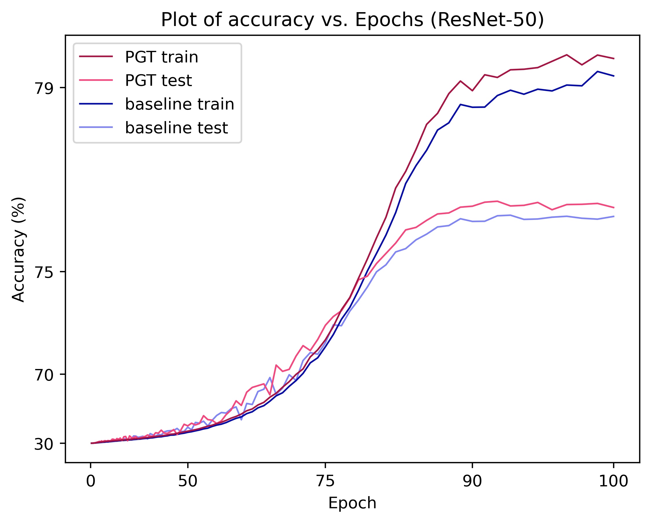
(b) Plot of training and test accuracies (ResNet-50)

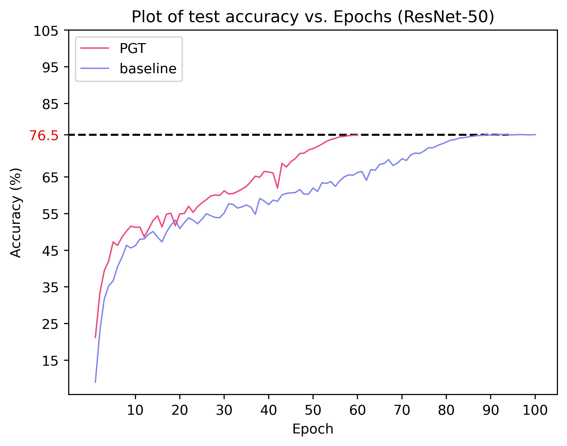
(c) Plot of test accuracies (ResNet-50)

Figure 4: Log-linear plots of training and test accuracies and comparison with baseline of batch-normalized variants: (a) ResNet-18 ($\alpha=0.25$), (b) ResNet-50 ($\alpha=0.3$). For better visualization of accuracies obtained in the final iterations, we plot both axes in log scale. PowerGrad Transform improves upon the baseline in all cases. The corresponding accuracies are mentioned in Table 1. (c) Training speed comparison between PGT ($60$ epochs) and baseline ($100$ epochs). They both converge to the same test accuracy ($76.5\%$) on ImageNet-1K. PGT’s accelerated training saves $40\%$ of the epoch budget.

Table 1: Results and comparison table for CNN networks trained on ImageNet-1K (sorted in descending order w.r.t. the last column denoting test accuracy improvements over baseline). Best training and test accuracies are highlighted in red and blue respectively. Accuracy differences are highlighted in yellow. In all experiments, we observe that PGT positively improves both training and test accuracies. We also observe that deeper networks such as SE-ResNet-50 and ResNet-50 accrue higher gains over the baselines as compared to shallow networks like ResNet-18.

Model	Scheduler	Method	PowerGrad	Train	Train	Test	Test
			Transform ($\alpha$)	Accuracy (%)	Diff (%)	Accuracy (%)	Diff (%)
SE-ResNet-50	Cosine	Baseline	-	81.5	+0.97	77.218	+0.734
		PGT	0.3	82.47		77.952
ResNet-50	Cosine	Baseline	-	79.18	+0.5	76.56	+0.656
		PGT	0.05	79.68		77.216
ResNet-50	Step	Baseline	-	78.99	+0.57	75.97	+0.524
		PGT	0.05	79.56		76.494
ResNet-101	Cosine	Baseline	-	82.29	+0.81	77.896	+0.362
		PGT	0.3	83.1		78.258
SE-ResNet-18	Cosine	Baseline	-	71.42	+0.18	71.09	+0.346
		PGT	0.25	71.6		71.436
ResNet-18	Step	Baseline	-	69.95	+0.35	69.704	+0.14
		PGT	0.25	70.3		69.844
ResNet-18	Cosine	Baseline	-	70.38	+0.15	70.208	+0.09
		PGT	0.25	70.53		70.298

We perform experiments on different variants ResNets using the ImageNet-1K dataset [7]. All models are trained on four V100 GPUs with a batch size of $1024$. We utilize a common set of hyperparameters for all experiments, which are as follows: 100 epoch budget, 5 epochs linear warmup phase beginning with a learning rate of $4\times 10^{-4}$ and ending with a peak learning rate of $0.4$, a momentum of $0.9$ and weight decay of $5\times 10^{-4}$, the SGD Nesterov optimizer and mixed precision. In our studies, we employ either a step scheduler (dividing the learning rate by $10$ at the $30^{th}$, $60^{th}$, and $90^{th}$ epochs) or a cosine decay scheduler [21]. We find $\alpha=0.25$ and $\alpha=0.05$ to be good choices for ResNet-18 and ResNet-50, though larger values such as $\alpha=0.3$ also have good performance as well. The experimental results are shown in Table 1, and we mention the value of the PGT hyperparmeter ($\alpha$) in each experiment. We explore different values of $\alpha$ in section 6 and provide detailed grid plots in the supplementary section.

In our experiments with Squeeze-and-Excitation variant of ResNet-50 i.e. SE-ResNet-50[16], we observe significant improvements; a $0.97\%$ boost in training accuracy and a $0.734\%$ increase in test accuracy. In our experiments with ResNet-50, we find an increase of $0.5\%$ and $0.656\%$ performance enhancement over the cosine scheduler baseline for training and testing respectively. The corresponding improvement over the step scheduler baseline for ResNet-50 is $0.57\%$ (training) and $0.524\%$ (testing). ResNet-101 sees a higher improvement in training fit, $0.81\%$ to be exact, while the improvement over the test set is $0.362\%$. Smaller networks such as SE-ResNet-18 and ResNet-18 sees accuracy boosts which are smaller but nevertheless positive. Therefore we conclude that with PGT, the consistent improvements in training accuracies across all cases is because the networks train better and arrive at better optimas during convergence. Per epoch training and test accuracy plots of ResNet-18 and ResNet-50 (both with and without PGT) are shown in Fig. 4(a, b). For better visualization of the top end of the plots, we scale both axes in log scale. Because both training and test accuracies improve, it indicates that PowerGrad Transform allows the network to learn better representations.

These improvements are obtained with the number of epochs being kept the same as that of the baseline model. Alternatively, practitioners can apply PGT and have the networks converge to accuracy levels comparable to the baseline with a significantly reduced epoch budget. In Fig. 4(c), we illustrate one such instance in which we train a ResNet-50 to its cosine scheduler baseline in just $60$ epochs with PGT, and match its baseline performance that is acquired in $100$ epochs. This hints to the observation that PGT not only makes the network perform better but also speeds up training. Because of the acceleration in training that is made possible by PGT, the total amount of training time can be decreased by $40\%$.

5.2 Empirical studies on networks without Batch Normalization

This section empirically examines some of the issues that occur when networks are trained without normalization layers and we provide insight into the effects of PowerGrad transform on such networks. We use ResNet-18 [13] as the foundation model for all empirical trials owing to its popularity among deep learning practitioners and the relative simplicity with which it can be trained on a big dataset such as ImageNet-1K [29]. We found deeper networks (such as ResNet-34 and ResNet-50 models) are impossible to train without BatchNormalization because of increased depth. So in order to conduct our empirical experiments, we solely focus on the ResNet-18 architecture. For our experiments, we designate different layers with their corresponding layer indices. We provide a detailed layer-wise index list of ResNet-18 in the supplementary section.

We concentrate on the following metric: the per-filter L2-norm of each layer’s weight tensor. Throughout the training process, we monitor variations in the per-filter weight norm. Because a full plot of each layer’s data would use an inordinate amount of space, we focus on a few critical layers’ plots. The supplementary section contains full plots for all layer for various settings. The norm of the weights of the $11^{\textit{th}}$ convolutional layer is shown in Fig. 5(a). Layer $11$ includes $256$ filters. Each colour on the figure represents the iteration-wise evolution of a particular filter throughout the course of training. The critical point to note is that some filters achieve a norm of zero during training. We refer to this event as ‘Zeroing Out’, and occurs when a channel of a weight tensor gets fully filled with zeros. If all the coefficients of the filter becomes zero, only then the L2 norm of that filter becomes zero. If we observe zero filter norm for a filter, then that filter does not contribute at all to determine the input-output relationship of a dataset, as the feature tensor it produces is also an all-zero tensor. According to our findings, when a filter tensor becomes zeroed out, it does not recover with further training. We observe both effects 1) zeroed out filter 2) zeroed out feature.

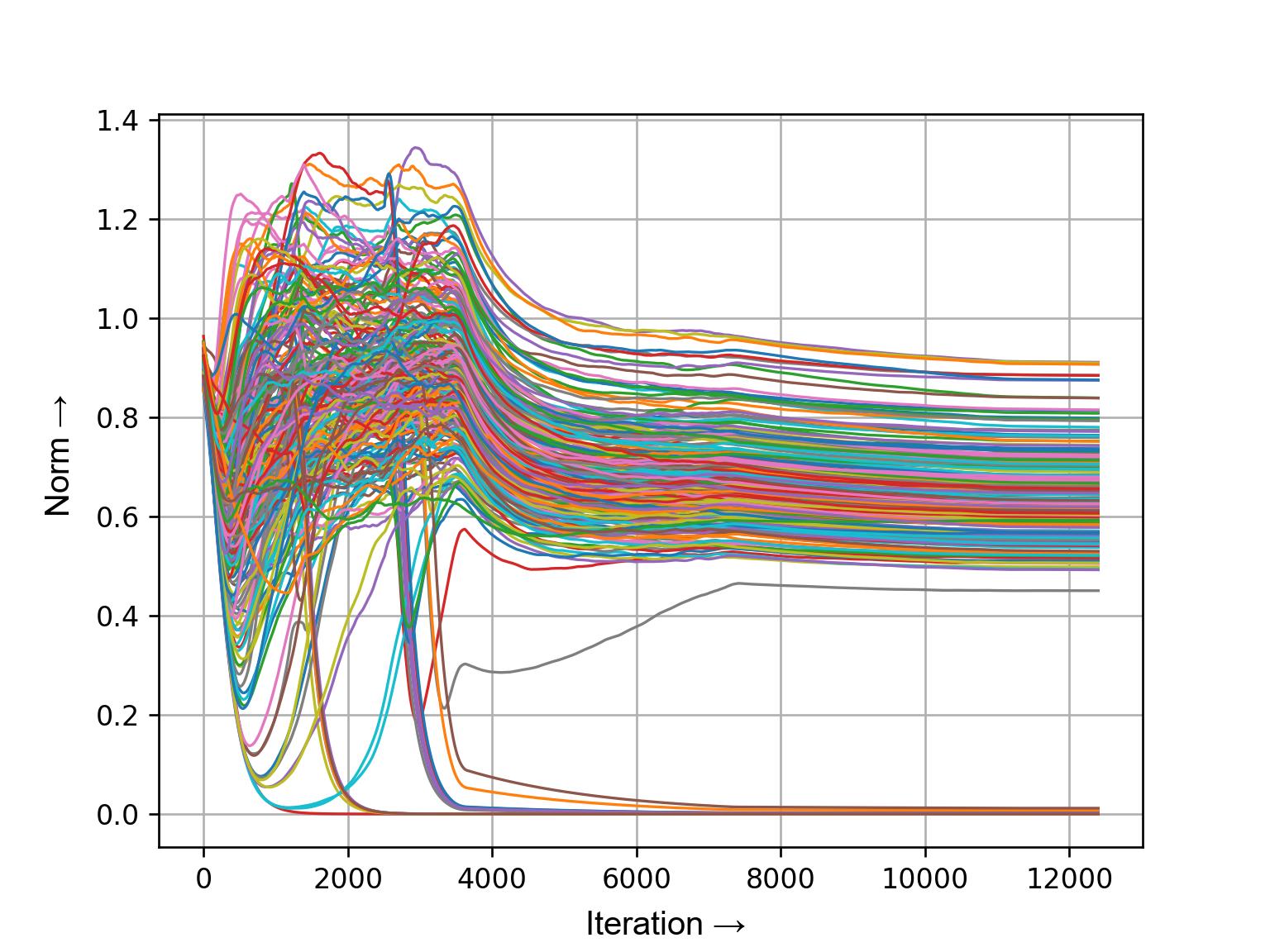
(a) Norm of filters of convolutional layer 11 (without PGT)

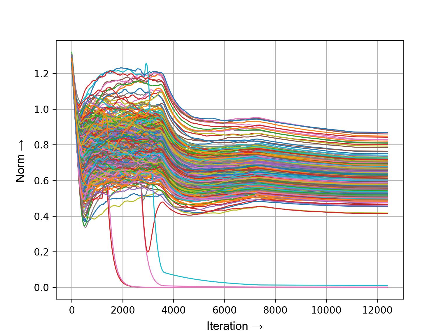
(b) Norm of filters of the final convolutional layer (without PGT)

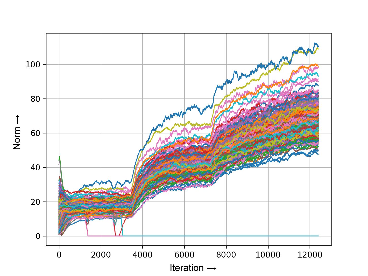
(c) Norm of final layer’s output features (without PGT)

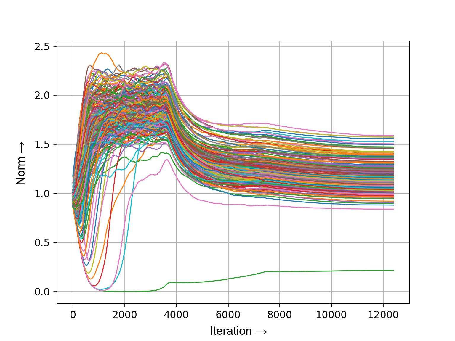
(d) Norm of filters of convolutional layer 11 (with PGT)

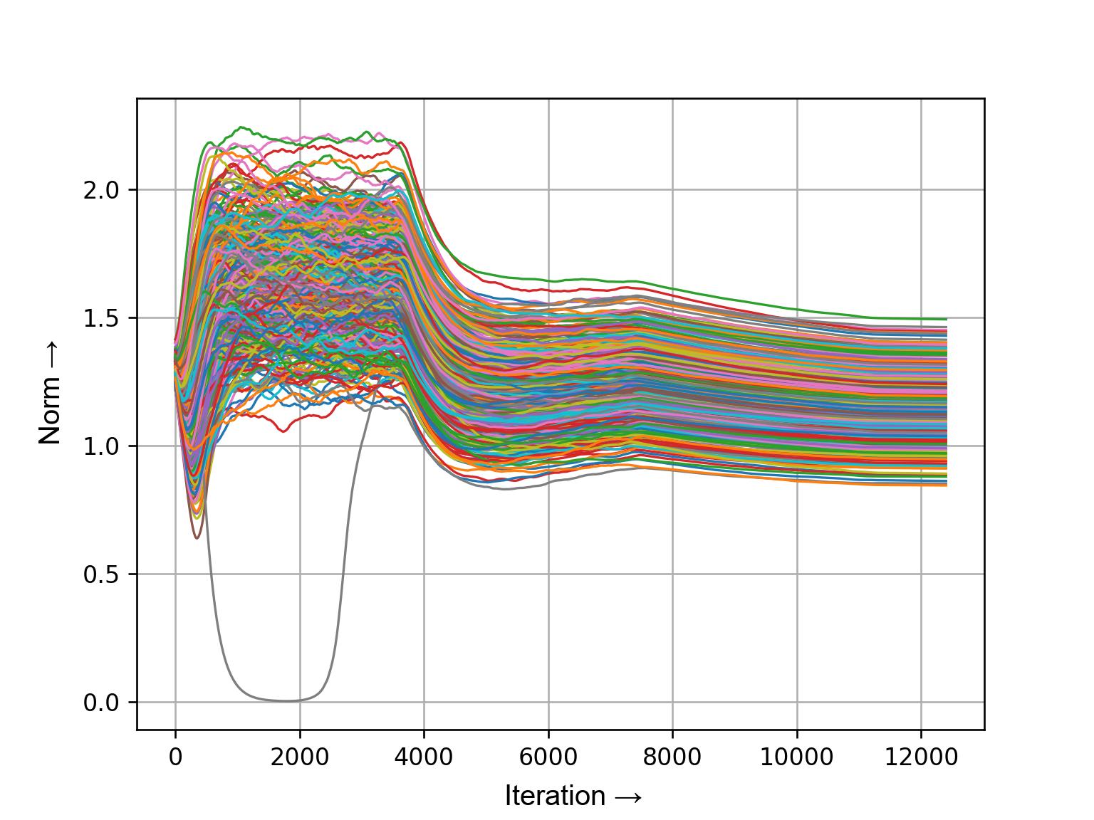
(e) Norm of filters of the final convolutional layer (with PGT)

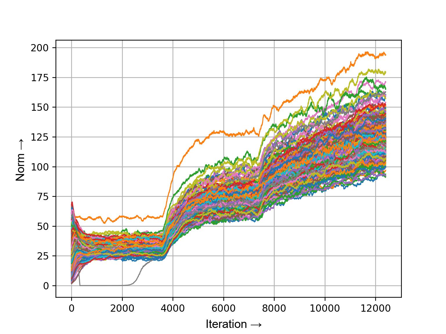
(f) Norm of final layer’s output features (with PGT)

Figure 5: Experiment demonstrating the Zeroing Out phenomena, as observed in different filters and feature vectors. PGT greatly reduces the zeroing out of filters and promote better learning.

Similar to the plot 5(a), we see the plot of the final convolutional layer in Fig. 5(b), where we observe a number of filters / units completely dropping out towards the end of training leading to underutilization of the network’s parameters. In Fig. 5(c), we see the norm of the feature vector at the output side of the global average pooling layer of ResNet-18. The feature vector here directly interfaces with the fully connected layer immediately after. Any zeroed out regions in this tensor directly leads to permanent information loss, as it does not contribute to the learning of decision boundaries in the upcoming fully connected layer, and indeed there exists a few zeroed out features in the baseline model, which we discuss next. The impact of having a zeroed out filter or a feature might have a variety of consequences for training and optimization. If a zeroed out filter is present in a convolutional layer, there are two possible outcomes. If the layer is immediately followed by a fully connected regression layer, there is an abrupt loss of information. For the reason that a zeroed out filter always generates zeroed out features regardless of the input image, when this tensor is fed to a fully connected layer, it does not communicate any information that is useful for classification. In the event that the zeroed out filter has a skip connection linked across it, this may be circumvented as long as there are no overlapping zeroed out channels in the two feature maps. On the other hand, if a feature tensor has a zeroed out channel at the input of a layer, the layer creates a zeroed out feature channel at the output, regardless of the weights. However, if there is a zeroed out channel in the feature map just before the fully connected layer, then this results in a permanent loss of information as it does not contribute to the learning of decision boundaries. ResNet-18 suffers from the same kind of information loss, as the final feature tensor (which is generated after the global average pooling layer) has multiple channels that are zeroed out [Fig. 5(c)]. This information collapse phenomenon occurs when a channel that has been zeroed out stays zeroed out for all images in the dataset.

Figure 6: Per filter norm vs. iteration plot of layer 5 of an unnormalized ResNet-18, trained with a very high batch size of 1024. The weight matrix of the entire layer zeroes out during training.

The impact of a feature tensor or weight tensor being zeroed out is seen to be particularly common in training procedures involving larger batch sizes in networks without normalization layers. As a result, the network’s parameters are underutilized since some of the filters are not involved in extracting any useful information that is important for performing classification. When working with large batch sizes, it is possible that an entire layer zeroes out [Fig. 6]. In a network without skip connections, this can cause a full collapse in training. For example, if a weight tensor completely zeroes out, and it always produces a zero feature tensor, then the input feature tensor to the next convolutional layer is a zero tensor and thus the output of the next layer is always a zero tensor irrespective of its weights, and this continues until the end of the neural network pipeline leading to zero logits. Also, zeroed out weights tensors lead to zeroed out gradients hence stopping training for all subsequent iterations leading to a collapse in training. Although residual networks bypass this difficulty via the use of the skip connection, it does not solve the layer’s non-participation in the overall objective of classification. It is possible to solve this issue by using methods such as gradient clipping (GC), adaptive gradient clipping (AGC), and PowerGrad Transform (PGT), all of which regulate the amount of gradient that flows at various junctions of the network. GC and AGC modify the gradients at each and every filter of every layer. PGT performs this operation at only one junction, which is at the softmax layer.

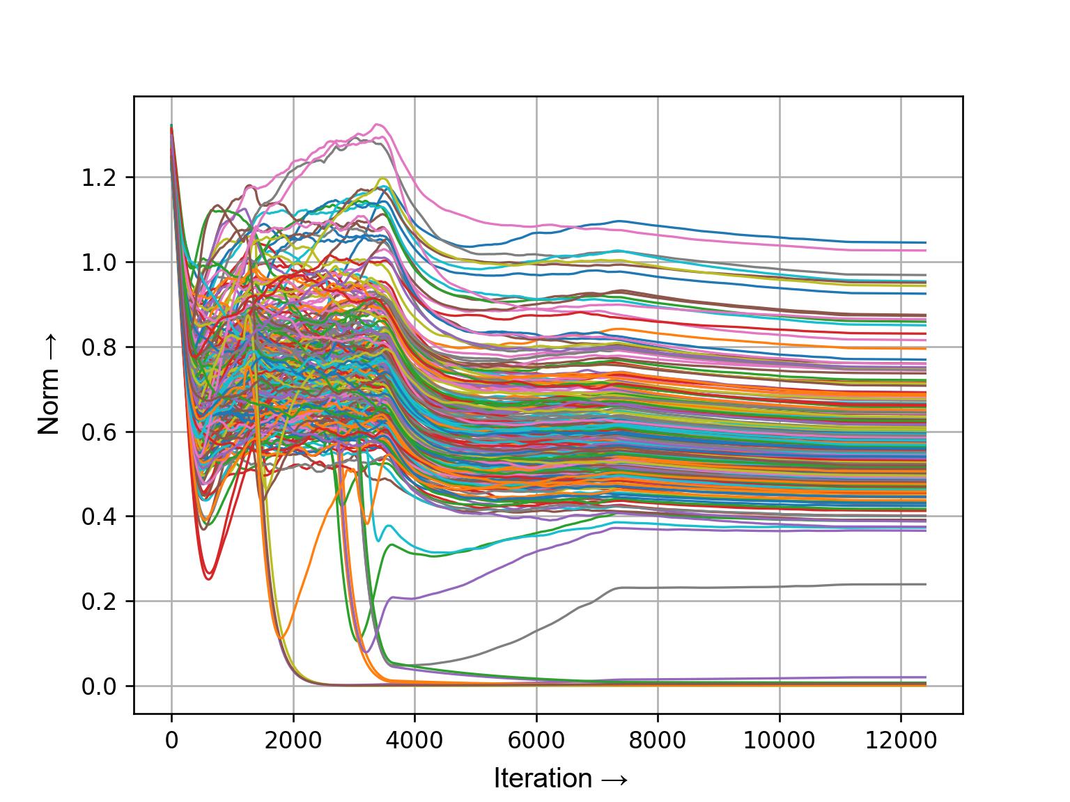
(a) Norm of filters of layer 15 (without AGC/PGT)

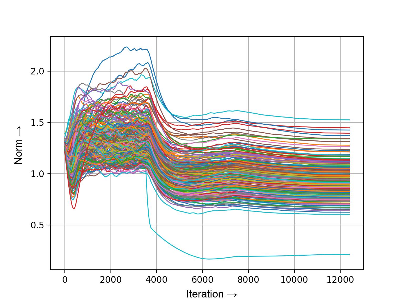
(b) Norm of filters of layer 15 (with PGT)

(c) Norm of filters of layer 15 (with AGC+PGT)

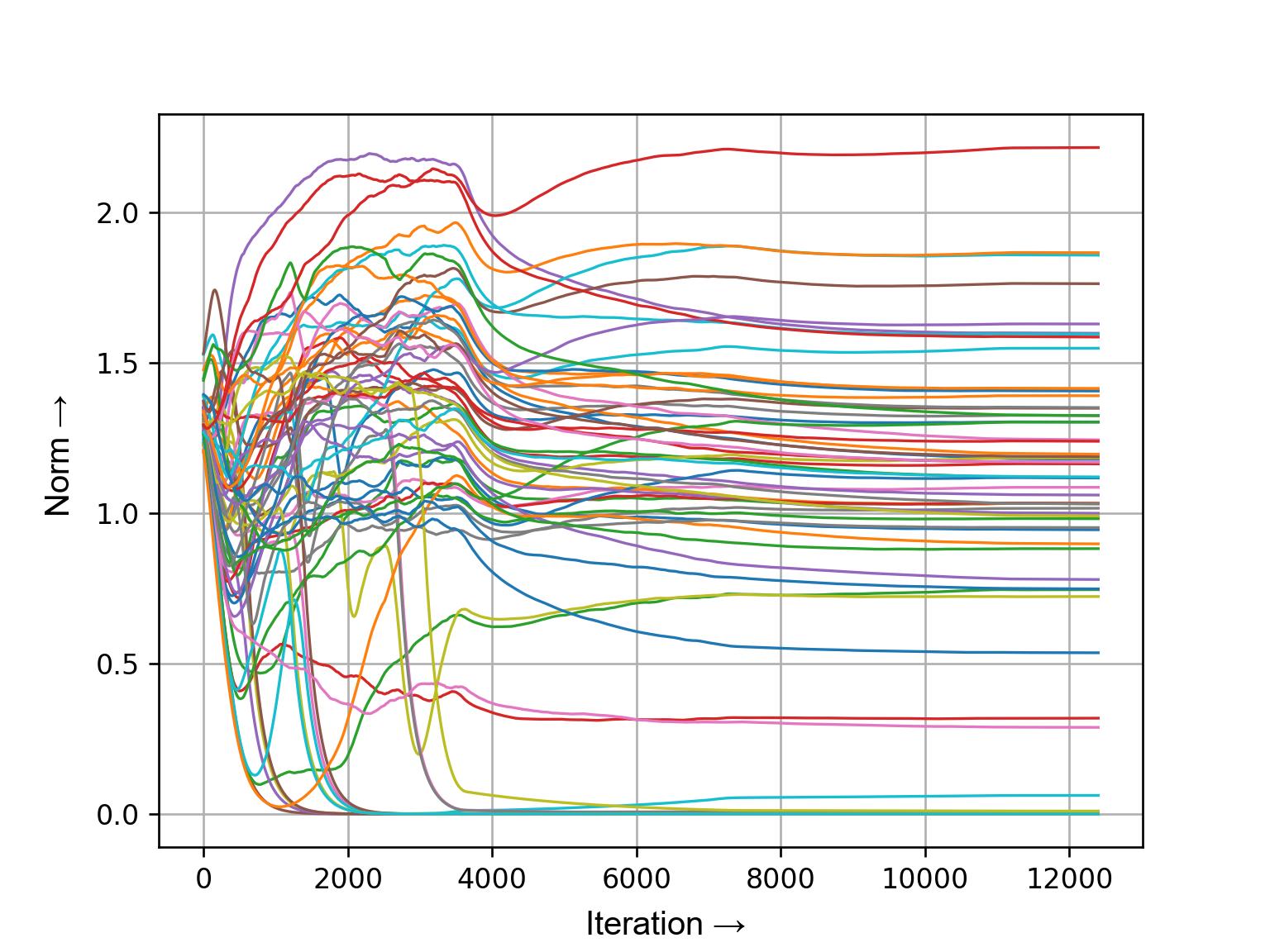
(d) Norm of filters of layer 2 (without AGC/PGT)

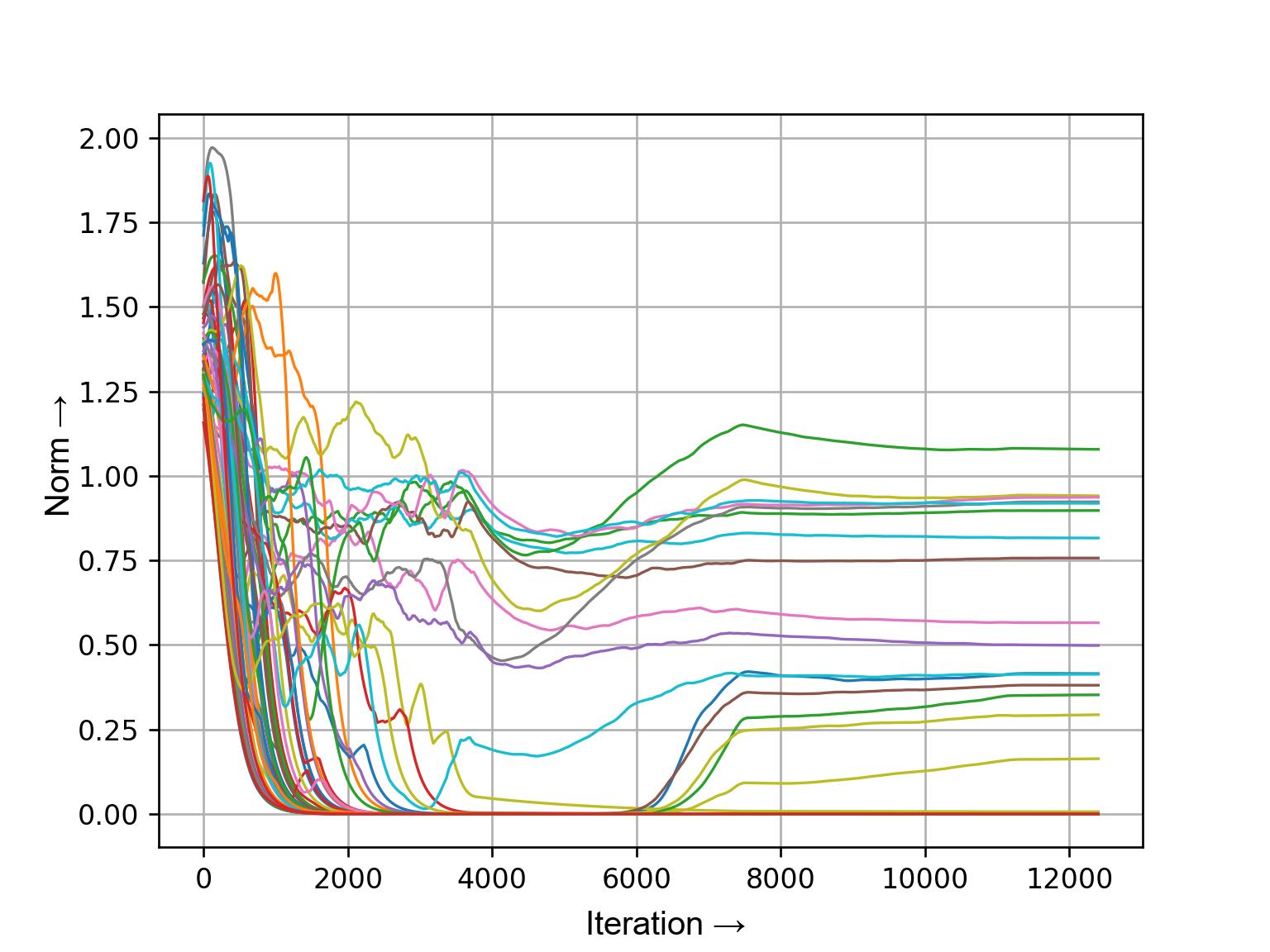
(e) Norm of filters of layer 2 (with PGT)

(f) Norm of filters of layer 2 (with AGC+PGT)

Figure 7: Experiment demonstrating the efficacy of PGT and AGC+PGT, as observed in different layers.

In a similar fashion to the study in section 5.2, we examine the norm profiles of features and weights in the PGT and AGC. The supplementary section includes all the detailed graphs of all layer. In Fig. 5(d), we show the per-filter norm plot of the $11^{\textit{th}}$ convolutional layer as it progresses through a PGT enabled training session. We observe that the number of zeroed out filters has considerably reduced. We observe similar benefits in plot of Fig. 5(e), which is the plot of the per-filter norm of the final convolutional layer. Coming to benefits in feature norms, we observe in plot of Fig. 5(f), the final feature tensor obtained with PGT enabled training do not contain any zeroed out regions, leading us to assert that information loss is heavily mitigated as the features pass on from the feature extracting convolutional layers to the fully connected stage for regression.

AGC is excellent at eliminating the issue of filter and feature zeroing out. However, AGC recovers a lower performance benefit than PGT. In the instance of PGT, we see that it also mitigates the zeroing out phenomenon in most layers. In Fig. 7(a), we see a plot of the $15^{\textit{th}}$ layer of the non-BN ResNet-18 trained without PGT. As we can see that there has been quite a few filter dropouts in the baseline. PGT recovers most of the filters [Fig. 7(b)]. In some layers however, the performance of PGT is slightly weaker than the baseline. The $2^{\textit{nd}}$ convolutional layer has more zeroed out filters in PGT [Fig. 7(e)] than in the baseline [Fig. 7(d)]. Despite that, PGT achieves a higher overall accuracy (Table 2). This necessitates the simultaneous use of AGC and PGT, for the non-BN ResNet-18.

Table 2: Results for non-normalized ResNets on ImageNet-1K. Each experiment is conducted with a 100 epoch budget using the cosine decay scheduler. Best training and test accuracies are highlighted in red and blue respectively. Top differences in training and test accuracies are marked in yellow. The baselines in each segment is taken as the reference point for all ‘Diff’ accuracies in that segment. The first three segments highlight comparison for experiments where the methods are applied individually, while the last segment denotes performance metrics for combinations of different methods (GC + PGT, AGC + PGT). We see that at any batch size, with PGT, the performance of non-normalized version of ResNet-18 improves significantly over the baseline owing to the improvements in training as observed in Fig. 7.

Model	Batch Size	Method	PowerGrad	Train	Train	Test	Test
			Transform ($\alpha$)	Accuracy (%)	Diff (%)	Accuracy (%)	Diff (%)
ResNet-18 (non-BN)	1024	Baseline	-	66.27	-	64.816	-
	1024	PGT	0.92	66.62	+0.35	65.498	+0.682
	512	Baseline	-	68.02	-	66.552	-
	512	PGT	0.25	69.5	+1.48	67.236	+0.684
	256	Baseline	-	68.86	-	66.796	-
	256	GC	-	69.04	+0.18	67.064	+0.268
	256	AGC	-	69.06	+0.2	67.298	+0.502
	256	PGT	0.25	69.97	+1.11	67.814	+1.018
	256	Baseline	-	68.86	-	66.796	-
	256	GC+PGT	0.25	68.67	-0.19	67.088	+0.292
	256	AGC+PGT	0.25	70.92	+2.06	68.856	+2.06

We provide performance metrics on the test set of ImageNet-1K for different batch sizes for the non-BN ResNet-18 and also experiment with different methods (GC, AGC, PGT along with their combinations). Table 2 shows the findings. To begin, we use a batch size of 1024. The baseline performance for this batch size is drastically inferior to baselines for other batch sizes. PGT helps regain some of the lost performance by $0.682\%$ ($65.498\%$ vs. $64.816\%$). This illustrates that in unnormalized networks, accuracy suffers significantly when batch sizes are large. Additionally, the training process is often unstable at this batch size, resulting in filters and sometimes entire layers frequently zeroing out (as seen in section 5.2). At a batch size of 512, invoking PGT improves the training accuracy baseline by $1.48\%$ and the test accuracy baseline by $0.684\%$, while at a batch size of 256, the improvement in training and test accuracies are $1.11\%$ and $1.018\%$ respectively. In comparison, the test accuracy improvements obtained by GC and AGC at batch size of 256 is much less, at $0.27\%$ and $0.5\%$, respectively.

On the training accuracy front, since we get a significant boost ($1.48\%$ at batch size of 512 and $1.11\%$ at batch size of 256), it leads us to infer that when PowerGrad Transform is used, the network fits the training dataset more tightly and the convergence optima is significantly superior. We also notice that the training versus testing gap increases with PGT as compared to the gap at baseline even though both training and test accuracies improve. Therefore it allows us to conclude that the improvements in training and test accuracies are obtained not through regularization like it does in methods such as label smoothing; rather the improvements are obtained as PGT enables the network to utilize its learning capacity better and arrive at a higher performing optima at convergence, something which is inaccessible through traditional gradient based training.

We also experiment with combinations of GC/AGC and PGT. The advantage of combining GC with PGT is not very significant. When AGC and PGT are combined, we see a tremendous increase in test accuracy of over $2.06\%$ over the baseline. As seen in Fig. 7(c) and 7(f), activating AGC and PGT concurrently results in no filter dropouts in all layers while also improving the accuracy by a significant margin. Additionally, we provide comprehensive graphs of the norm profiles of the AGC + PGT method for all layers in the supplementary section.

5.3 Effect on Loss, Logits and other metrics

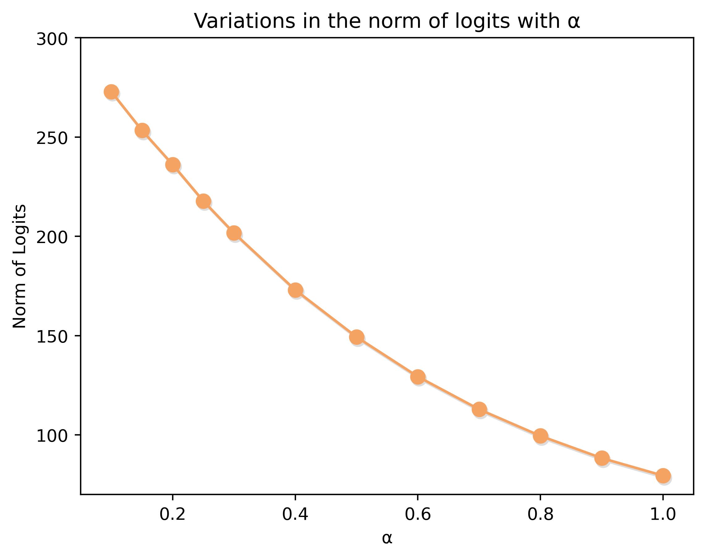
(a)
Logit vs. $\alpha$

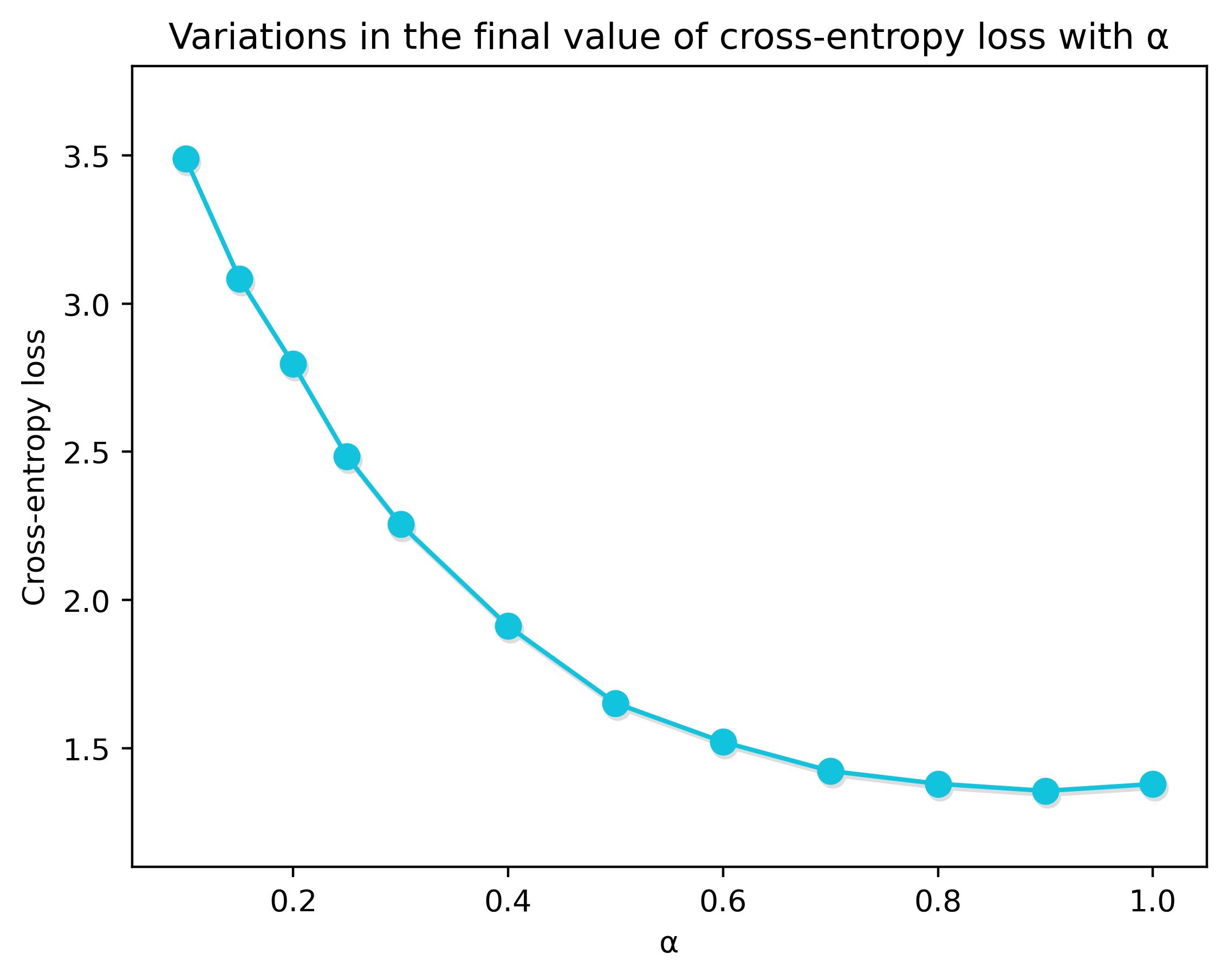
(b)
Cross-entropy loss vs. $\alpha$

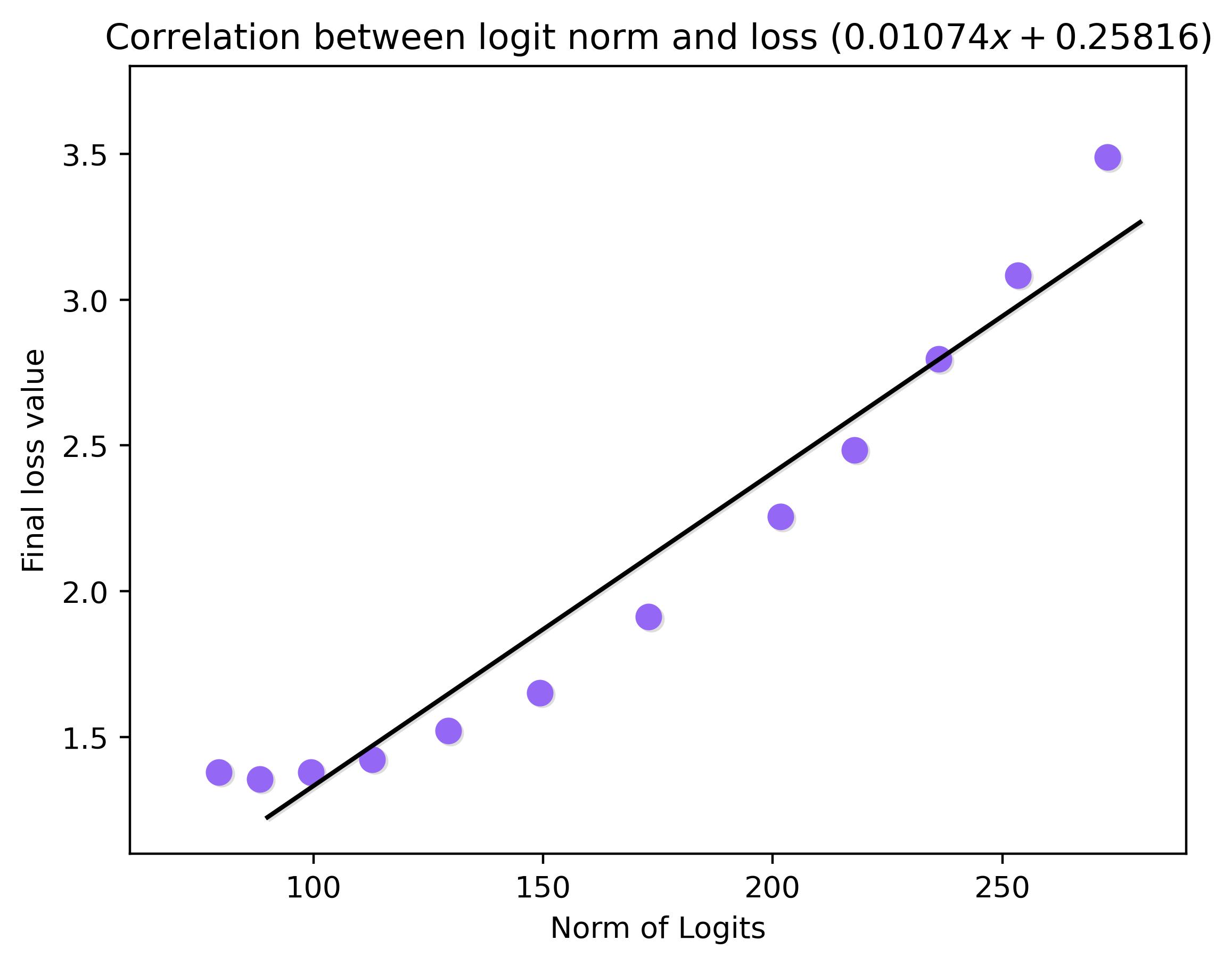
(c)
Logit-Loss correlation

Figure 8: Plots of various statistical measures: (a) Variations in the logit norm vs. $\alpha$. The logit norm is calculated per image over the test set of ImageNet-1K (at the linear layer of the ResNet-18 architecture) and then averaged. (b) Variations in the final loss values obtained for different $\alpha$ settings. (c) Correlation between loss and logits. Regression line equation :$(0.01074x+0.25816)$.

As seen in Fig. 8(a), the logit norm increases as $\alpha$ falls from $1$ to $0$. In the initial training phase, PGT causes the gradient in both the valid and wrong classes to rise as the network misclassifies majority of the examples. Due to the exponential nature of the softmax function, the predicted probability distribution may frequently be close to a delta distribution, even in instances of misclassifications. PGT reshapes the predicted probability distribution. It redistributes probability from the confident classes to the less confident ones. Gradient rises in all classes. We also see that the final value of the loss rises as $\alpha$ drops, and that the logit norm and the final value of the loss are linearly correlated Fig. 8(c). What is surprising is that: it is possible to achieve higher accuracies even though the loss values are larger during convergence. In our studies with ResNet-50, for instance, if PGT is not invoked, the corresponding test accuracy is $76.56\%$ (Table 1) with a cross-entropy loss value of $0.852$. However, if PGT is activated with $\alpha=0.05$, the corresponding test accuracy is $77.216\%$ (Table 1) with a loss value of $2.360$. This is markedly different from the coupled gradient descent based training procedures. PGT enables the network to arrive at such optima where the loss values are high, but both training and test perfomance is better. From these plots of logits and losses we find that with the inclusion of PGT in the training process, the model can have access to such regions of the loss landscape that is otherwise inaccessible to traditional gradient based training procedures.

6 Ablation Study

Table 3: Ablation study for ResNet-50 on ImageNet-1K. LS column denotes whether label smoothing has been applied. A smoothing hyperparameter value of $0.1$ has been used. The hyperparameter column that controls the amount of PGT gradient modification injected at softmax, Eq. 8.

#Row	Model	Scheduler	Label	PowerGrad	Train	Test	Gap (%)
			Smoothing	Transform ($\alpha$)	Accuracy (%)	Accuracy (%)
1.	ResNet-50	Step	✗	✗	78.99	75.97	3.02
2.	ResNet-50	Step	✗	0.3	79.56	76.494	3.066
3.	ResNet-50	Cosine	✗	✗	79.18	76.56	2.62
4.	ResNet-50	Cosine	0.1	✗	78.81	76.698	2.112
5.	ResNet-50	Cosine	✗	0.3	79.43	76.886	2.544
6.	ResNet-50	Cosine	0.1	0.3	78.47	76.968	1.502
7.	ResNet-50	Cosine	✗	0.05	79.68	77.216	2.464
8.	ResNet-50	Cosine	0.1	0.05	77.69	76.39	1.3

We conduct an ablation study to investigate the effects of PowerGrad Transform for different values of the hyperparameter ($\alpha$). Grid plots are made available in the supplementary section. We have previously demonstrated from the experiments depicted in section 5, that PowerGrad Transform causes the network to arrive at a better optima and fit the training dataset better than the baseline. In this ablation study, we use the ResNet-50 architecture and we combine our proposed method with other regularization techniques such as label smoothing and report our findings in Table 3. We also investigate the two optimal peaks of the hyperparameter ($\alpha$) obtained from ResNet-50’s grid search ($\alpha=0.05$ and $\alpha=0.3$). First, we examine the effect of PGT on the step scheduler baseline in order to later compare it to the cosine scheduler baseline. Row-1) We begin with the step scheduler baseline ($75.97\%$). Row-2) PGT improves upon the step scheduler baseline (test set) by a substantial margin with $0.524\%$ ($76.494\%$ as opposed to $75.97\%$). Row-3) Introducing the cosine scheduler yields a $0.59\%$ improvement ($76.56\%$ vs. $75.97\%$) over the step scheduler. Row-4) After introducing label smoothing, the test accuracy relative to the cosine scheduler baseline increases by only $0.138\%$ (from $76.56\%$ to $76.698\%$). Row-5) However, introducing PGT with $\alpha=0.3$ alone (without label smoothing) improves the cosine scheduler baseline by $0.326\%$ ($76.886\%$ vs. $76.56\%$). Row-6) Combining PGT ($\alpha=0.3$) with label smoothing improves the performance on the test set further by $0.408\%$ (from $76.56\%$ to $76.968\%$) and reduces the generalization gap (from $2.54\%$ to $1.5\%$). However, the impact of combining PGT with label smoothing can vary depending on the value of the hyperparameter ($\alpha$). Row-7) With a PGT hyperparameter value of $\alpha=0.05$, we notice the greatest performance improvement, $1.246\%$ over the step scheduler test baseline and $0.656\%$ over the cosine scheduler test baseline. Row-8) Adding label smoothing to PGT ($\alpha=0.05$) hurts performance even though it reduces the generalization gap.

7 Discussions

We introduced PowerGrad Transform, which decouples the backward and forward passes of neural network training and enables a significantly better fit to the dataset, as measured by training and test accuracy metrics. We show the application of PowerGrad Transform, a simple yet powerful technique for modifying the gradient flow behaviour. We investigate experimentally the degenerate behavior of non-BN networks, which is frequently observed during the standard training approach, especially with higher batch sizes. With PGT, gradient behavior is enhanced and the likelihood of weights attaining degenerate states is diminished. We provide a theoretical analysis of the PowerGrad transformation. With the use of different network topologies and datasets, we are able to show the potential of PGT and explore its impacts from an empirical standpoint. We provide comprehensive results on a number of models (non-BN and BN ResNets, SE-ResNets) using the ImageNet dataset. PGT helps the network to improve its learning capabilities by locating a more optimum convergence point and simultaneously speeds up training. In addition, we undertake an ablation research and compare its effects to those of regularization methods such label smoothing.

8 Supplementary section

8.1 Sample Code

In PyTorch, the available method to modify gradients in the backward pass is using the register_hook function which is called in the forward function.

 

⬇

# Modification of gradients take place

# inside the forward function

def forward(self, x, labels):

# x: Input tensor with shape [N, C, H, W]

# labels: One hot ground truth with shape [N, C]

logits = self.layers(x)

def powerGradTransform(grad):

alpha = 0.3

# Recover the predicted probabilites

# generated in the forward pass

grad_temp = grad / grad.shape[0]

pred = grad_temp + labels

# Transform the predicted probabilities

pred = pred**alpha

pred /= pred.sum(-1, keepdim=True)

# Modify the gradient

modified_grad = pred - labels

modified_grad = modified_grad * grad.shape[0]

return modified_grad

if self.training:

logits.register_hook(powerGradTransform)

return logits

Figure 9: Python code of PowerGrad Transform based on PyTorch.

 

8.2 Grid search for different values of $\alpha$

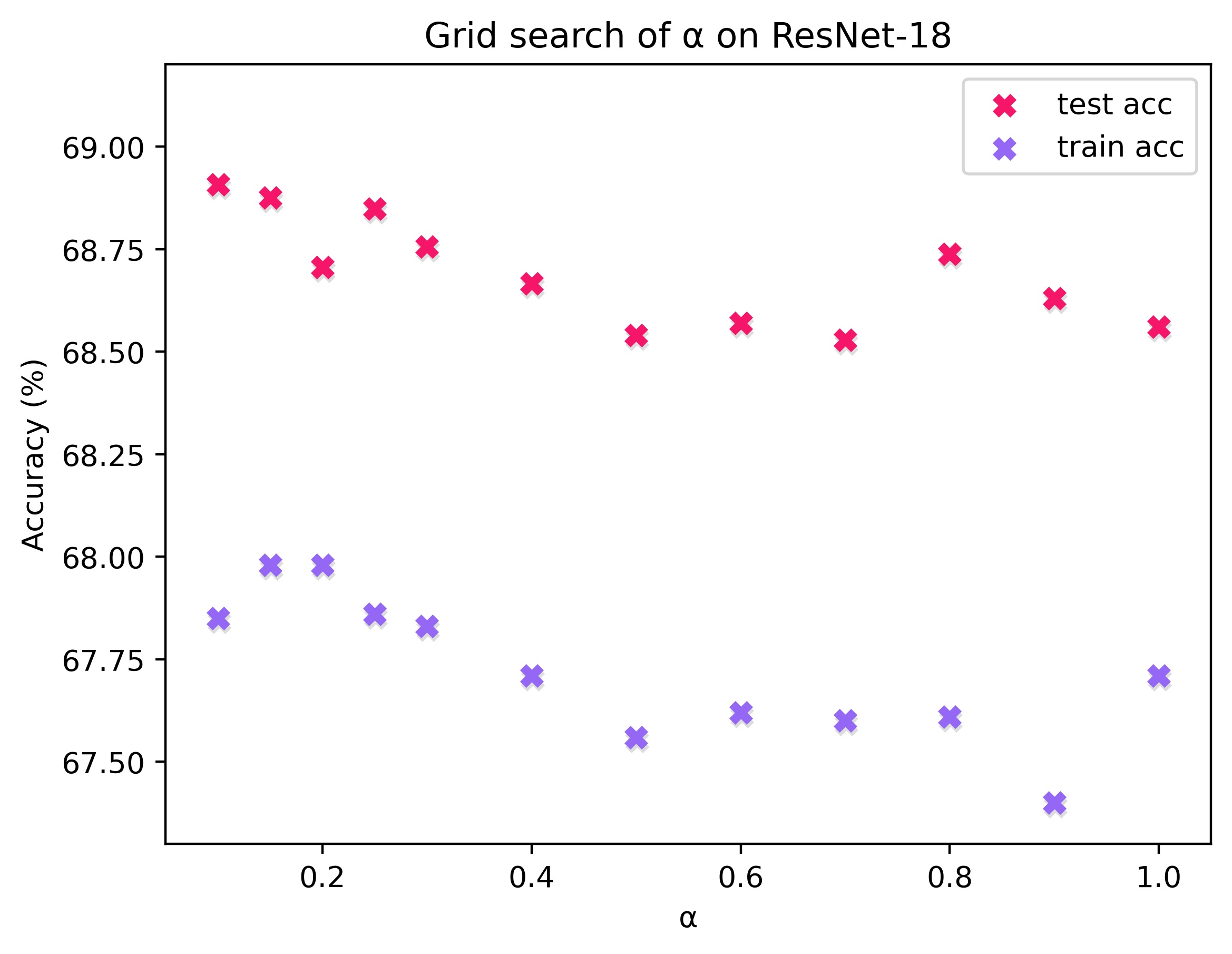
Figure 10: Grid search for various values of $\alpha$ for ResNet-18 architecture with the ImageNet dataset. Each datapoint is collected over a 50 epoch budget, with other hyperparameters kept the same as mentioned in section 5.1.

Figure 11: Grid search for various values of $\alpha$ for ResNet-50 architecture with the ImageNet dataset. Each datapoint is collected over a 50 epoch budget, with other hyperparameters kept the same as mentioned in section 5.1.

Figure 12:
ResNet-20 CIFAR-10

Figure 13: Grid search for various values of $\alpha$ for ResNet-20 architecture with the CIFAR-10 dataset. Each datapoint is collected over a 360 epoch budget.

There is no effect of PGT on small datasets such as CIFAR-10. In these scenarios, networks almost always achieve $100\%$ training accuracy, leaving no room for PGT to assist.

8.3 Norm plots of weights (baseline (low batch size)) of non-BN ResNet-18

Figure 14: Method: baseline, batch size = 256. This is a plot depicting the iteration-wise evolution of the norm of each filter in each layer. Each subplot corresponds to a layer of the unnormalized ResNet-18. Above each subplot, the layer indices are shown. Each filter in each subplot is shown with a separate and randomly determined colour.

8.4 Norm plots of weights (baseline (high batch size)) of non-BN ResNet-18

Figure 15: Method: baseline (high batch size), batch size = 1024. This is a plot depicting the iteration-wise evolution of the norm of each filter in each layer. Each subplot corresponds to a layer of the unnormalized ResNet-18. Above each subplot, the layer indices are shown. Each filter in each subplot is shown with a separate and randomly determined colour.

8.5 Norm plots of weights (PGT) of non-BN ResNet-18

Figure 16: Method: PGT, batch size = 256. This is a plot depicting the iteration-wise evolution of the norm of each filter in each layer. Each subplot corresponds to a layer of the unnormalized ResNet-18. Above each subplot, the layer indices are shown. Each filter in each subplot is shown with a separate and randomly determined colour.

8.6 Norm plots of weights (AGC + PGT) of non-BN ResNet-18

Figure 17: Method: AGC + PGT, batch size = 256. This is a plot depicting the iteration-wise evolution of the norm of each filter in each layer. Each subplot corresponds to a layer of the unnormalized ResNet-18. Above each subplot, the layer indices are shown. Each filter in each subplot is shown with a separate and randomly determined colour.

8.7 ResNet-18 Layer Index Diagram

For the layer indices used in figures Fig. 5, 6, 7, we provide a block diagram depicting the different convolutional layers of ResNet-18 with corresponding layer indices in Fig. 18. Each layer represents a convolutional layer, with the layer index and the number of filters denoted alongside it. Downsampling convolutional layers in skip connections are drawn and their layer indices are shown on the skip connection paths.

ResNet-18 is composed of $20$ convolutional layers and one fully connected (FC) layer. At the input, it has a single convolutional layer with filters of size $7\times 7$. Three convolutional layers are placed in the downsampling skip connections. The remaining convolutional layers have several $3\times 3$ filters that are grouped together to create a block. Each basic block is connected by a skip connection. At the end of all convolutional layers, a global average pooling layer downsamples the features to a fixed-size feature vector and transfers it to the FC layer, which fits the features using regression and outputs logits. The logits $z_{i}$ produced by the FC layer are fed into a softmax layer, which transforms them to predicted probabilities $p_{i}$ using the equation $p_{i}=\frac{e^{z_{i}}}{\sum_{j}e^{z_{j}}}$.

Figure 18: ResNet-18 architecture with layer indices of convolutional layers and the number of filters in each layer.

References

- [1] Gustavo Aguilar, Yuan Ling, Yu Zhang, Benjamin Yao, Xing Fan, and Chenlei Guo. Knowledge distillation from internal representations. In Proceedings of the AAAI Conference on Artificial Intelligence, volume 34, pages 7350–7357, 2020.
- [2] Maxwell M Aladago and Lorenzo Torresani. Slot machines: Discovering winning combinations of random weights in neural networks. In International Conference on Machine Learning, pages 163–174. PMLR, 2021.
- [3] Jimmy Ba and Rich Caruana. Do deep nets really need to be deep? In Zoubin Ghahramani, Max Welling, Corinna Cortes, Neil D. Lawrence, and Kilian Q. Weinberger, editors, Advances in Neural Information Processing Systems 27: Annual Conference on Neural Information Processing Systems 2014, December 8-13 2014, Montreal, Quebec, Canada, pages 2654–2662, 2014.
- [4] Andrew Brock, Soham De, Samuel L Smith, and Karen Simonyan. High-performance large-scale image recognition without normalization. arXiv preprint arXiv:2102.06171, 2021.
- [5] Jang Hyun Cho and Bharath Hariharan. On the efficacy of knowledge distillation. In Proceedings of the IEEE/CVF International Conference on Computer Vision, pages 4794–4802, 2019.
- [6] Jan Chorowski and Navdeep Jaitly. Towards better decoding and language model integration in sequence to sequence models. arXiv preprint arXiv:1612.02695, 2016.
- [7] Jia Deng, Wei Dong, Richard Socher, Li-Jia Li, Kai Li, and Li Fei-Fei. Imagenet: A large-scale hierarchical image database. In 2009 IEEE conference on computer vision and pattern recognition, pages 248–255. Ieee, 2009.
- [8] Abhimanyu Dubey, Otkrist Gupta, Pei Guo, Ramesh Raskar, Ryan Farrell, and Nikhil Naik. Pairwise confusion for fine-grained visual classification. In Proceedings of the European conference on computer vision (ECCV), pages 70–86, 2018.
- [9] John Duchi, Elad Hazan, and Yoram Singer. Adaptive subgradient methods for online learning and stochastic optimization. Journal of machine learning research, 12(7), 2011.
- [10] Tommaso Furlanello, Zachary Lipton, Michael Tschannen, Laurent Itti, and Anima Anandkumar. Born again neural networks. In International Conference on Machine Learning, pages 1607–1616. PMLR, 2018.
- [11] Shiming Ge, Zhao Luo, Chunhui Zhang, Yingying Hua, and Dacheng Tao. Distilling channels for efficient deep tracking. IEEE Transactions on Image Processing, 29:2610–2621, 2019.
- [12] Shiming Ge, Shengwei Zhao, Chenyu Li, and Jia Li. Low-resolution face recognition in the wild via selective knowledge distillation. IEEE Transactions on Image Processing, 28(4):2051–2062, 2018.
- [13] Kaiming He, Xiangyu Zhang, Shaoqing Ren, and Jian Sun. Deep residual learning for image recognition. In Proceedings of the IEEE conference on computer vision and pattern recognition, pages 770–778, 2016.
- [14] Yu-Lin He, Xiao-Liang Zhang, Wei Ao, and Joshua Zhexue Huang. Determining the optimal temperature parameter for softmax function in reinforcement learning. Applied Soft Computing, 70:80–85, 2018.
- [15] Geoffrey Hinton, Oriol Vinyals, and Jeff Dean. Distilling the knowledge in a neural network. arXiv preprint arXiv:1503.02531, 2015.
- [16] Jie Hu, Li Shen, and Gang Sun. Squeeze-and-excitation networks. In Proceedings of the IEEE conference on computer vision and pattern recognition, pages 7132–7141, 2018.
- [17] Yann LeCun, D Touresky, G Hinton, and T Sejnowski. A theoretical framework for back-propagation. In Proceedings of the 1988 connectionist models summer school, volume 1, pages 21–28, 1988.
- [18] Timothy P Lillicrap, Adam Santoro, Luke Marris, Colin J Akerman, and Geoffrey Hinton. Backpropagation and the brain. Nature Reviews Neuroscience, 21(6):335–346, 2020.
- [19] Weiyang Liu, Yandong Wen, Zhiding Yu, Ming Li, Bhiksha Raj, and Le Song. Sphereface: Deep hypersphere embedding for face recognition. In Proceedings of the IEEE conference on computer vision and pattern recognition, pages 212–220, 2017.
- [20] Xuan Liu, Xiaoguang Wang, and Stan Matwin. Improving the interpretability of deep neural networks with knowledge distillation. In 2018 IEEE International Conference on Data Mining Workshops (ICDMW), pages 905–912. IEEE, 2018.
- [21] Ilya Loshchilov and Frank Hutter. Sgdr: Stochastic gradient descent with warm restarts. arXiv preprint arXiv:1608.03983, 2016.
- [22] Stephen Merity, Nitish Shirish Keskar, and Richard Socher. Regularizing and optimizing lstm language models. arXiv preprint arXiv:1708.02182, 2017.
- [23] Rafael Müller, Simon Kornblith, and Geoffrey E. Hinton. When does label smoothing help? In Hanna M. Wallach, Hugo Larochelle, Alina Beygelzimer, Florence d’Alché-Buc, Emily B. Fox, and Roman Garnett, editors, Advances in Neural Information Processing Systems 32: Annual Conference on Neural Information Processing Systems 2019, NeurIPS 2019, December 8-14, 2019, Vancouver, BC, Canada, pages 4696–4705, 2019.
- [24] Razvan Pascanu, Tomas Mikolov, and Yoshua Bengio. Understanding the exploding gradient problem. CoRR, abs/1211.5063, 2(417):1, 2012.
- [25] Razvan Pascanu, Tomas Mikolov, and Yoshua Bengio. On the difficulty of training recurrent neural networks. In International conference on machine learning, pages 1310–1318. PMLR, 2013.
- [26] Nikolaos Passalis and Anastasios Tefas. Unsupervised knowledge transfer using similarity embeddings. IEEE transactions on neural networks and learning systems, 30(3):946–950, 2018.
- [27] Adam Paszke, Sam Gross, Francisco Massa, Adam Lerer, James Bradbury, Gregory Chanan, Trevor Killeen, Zeming Lin, Natalia Gimelshein, Luca Antiga, Alban Desmaison, Andreas Kopf, Edward Yang, Zachary DeVito, Martin Raison, Alykhan Tejani, Sasank Chilamkurthy, Benoit Steiner, Lu Fang, Junjie Bai, and Soumith Chintala. Pytorch: An imperative style, high-performance deep learning library. In H. Wallach, H. Larochelle, A. Beygelzimer, F. d'Alché-Buc, E. Fox, and R. Garnett, editors, Advances in Neural Information Processing Systems 32, pages 8024–8035. Curran Associates, Inc., 2019.
- [28] Scott Reed, Honglak Lee, Dragomir Anguelov, Christian Szegedy, Dumitru Erhan, and Andrew Rabinovich. Training deep neural networks on noisy labels with bootstrapping. arXiv preprint arXiv:1412.6596, 2014.
- [29] Olga Russakovsky, Jia Deng, Hao Su, Jonathan Krause, Sanjeev Satheesh, Sean Ma, Zhiheng Huang, Andrej Karpathy, Aditya Khosla, Michael Bernstein, et al. Imagenet large scale visual recognition challenge. International journal of computer vision, 115(3):211–252, 2015.
- [30] Samuel Smith, Erich Elsen, and Soham De. On the generalization benefit of noise in stochastic gradient descent. In International Conference on Machine Learning, pages 9058–9067. PMLR, 2020.
- [31] Christian Szegedy, Vincent Vanhoucke, Sergey Ioffe, Jon Shlens, and Zbigniew Wojna. Rethinking the inception architecture for computer vision. In Proceedings of the IEEE conference on computer vision and pattern recognition, pages 2818–2826, 2016.
- [32] Hao Wang, Yitong Wang, Zheng Zhou, Xing Ji, Dihong Gong, Jingchao Zhou, Zhifeng Li, and Wei Liu. Cosface: Large margin cosine loss for deep face recognition. In Proceedings of the IEEE conference on computer vision and pattern recognition, pages 5265–5274, 2018.
- [33] Jiyue Wang, Pei Zhang, and Yanxiong Li. Memory-replay knowledge distillation. Sensors, 21(8):2792, 2021.
- [34] Ning Wang, Wengang Zhou, Yibing Song, Chao Ma, and Houqiang Li. Real-time correlation tracking via joint model compression and transfer. IEEE Transactions on Image Processing, 29:6123–6135, 2020.
- [35] Ross Wightman. Pytorch image models. https://github.com/rwightman/pytorch-image-models, 2019.
- [36] Zhirong Wu, Alexei A Efros, and Stella X Yu. Improving generalization via scalable neighborhood component analysis. In Proceedings of the European Conference on Computer Vision (ECCV), pages 685–701, 2018.
- [37] Lingxi Xie, Jingdong Wang, Zhen Wei, Meng Wang, and Qi Tian. Disturblabel: Regularizing cnn on the loss layer. In Proceedings of the IEEE Conference on Computer Vision and Pattern Recognition, pages 4753–4762, 2016.
- [38] Ting-Bing Xu and Cheng-Lin Liu. Data-distortion guided self-distillation for deep neural networks. In Proceedings of the AAAI Conference on Artificial Intelligence, volume 33, pages 5565–5572, 2019.
- [39] Jiangchao Yao, Jiajie Wang, Ivor W Tsang, Ya Zhang, Jun Sun, Chengqi Zhang, and Rui Zhang. Deep learning from noisy image labels with quality embedding. IEEE Transactions on Image Processing, 28(4):1909–1922, 2018.
- [40] Li Yuan, Francis EH Tay, Guilin Li, Tao Wang, and Jiashi Feng. Revisiting knowledge distillation via label smoothing regularization. In Proceedings of the IEEE/CVF Conference on Computer Vision and Pattern Recognition, pages 3903–3911, 2020.
- [41] Sukmin Yun, Jongjin Park, Kimin Lee, and Jinwoo Shin. Regularizing class-wise predictions via self-knowledge distillation. In Proceedings of the IEEE/CVF conference on computer vision and pattern recognition, pages 13876–13885, 2020.
- [42] Andrew Zhai and Hao-Yu Wu. Classification is a strong baseline for deep metric learning. arXiv preprint arXiv:1811.12649, 2018.
- [43] Jingzhao Zhang, Tianxing He, Suvrit Sra, and Ali Jadbabaie. Why gradient clipping accelerates training: A theoretical justification for adaptivity. arXiv preprint arXiv:1905.11881, 2019.
- [44] Linfeng Zhang, Jiebo Song, Anni Gao, Jingwei Chen, Chenglong Bao, and Kaisheng Ma. Be your own teacher: Improve the performance of convolutional neural networks via self distillation. In Proceedings of the IEEE/CVF International Conference on Computer Vision, pages 3713–3722, 2019.
- [45] Ying Zhang, Tao Xiang, Timothy M Hospedales, and Huchuan Lu. Deep mutual learning. In Proceedings of the IEEE Conference on Computer Vision and Pattern Recognition, pages 4320–4328, 2018.