Matching Learned Causal Effects of Neural Networks with Domain Priors

Abstract

A trained neural network can be interpreted as a structural causal model (SCM) that provides the effect of changing input variables on the model’s output. However, if training data contains both causal and correlational relationships, a model that optimizes prediction accuracy may not necessarily learn the true causal relationships between input and output variables. On the other hand, expert users often have prior knowledge of the causal relationship between certain input variables and output from domain knowledge. Therefore, we propose a regularization method that aligns the learned causal effects of a neural network with domain priors, including both direct and total causal effects. We show that this approach can generalize to different kinds of domain priors, including monotonicity of causal effect of an input variable on output or zero causal effect of a variable on output for purposes of fairness. Our experiments on twelve benchmark datasets show its utility in regularizing a neural network model to maintain desired causal effects, without compromising on accuracy. Importantly, we also show that a model thus trained is robust and gets improved accuracy on noisy inputs.

1 Introduction

There has been a growing interest in integrating causal principles into machine learning models in recent years. Existing efforts have largely focused on post-hoc explanations of a trained neural network (NN) model’s decisions in terms of causal effect (Chattopadhyay et al., 2019; Goyal et al., 2019a), using counterfactuals for explanations or augmentations (Goyal et al., 2019b; Zmigrod et al., 2019; Pitis et al., 2020; Dash et al., 2022), causal discovery (Zhu et al., 2020), or embedding causal structures in disentangled representation learning (Suter et al., 2019; Yang et al., 2020). However, while there have been efforts of quantifying the causal attributions learned by an NN (Chattopadhyay et al., 2019; Goyal et al., 2019a), none of these efforts consider the possibility that expert human users that interact with NN models in practice may have prior knowledge of relationships between input and output variables, even causal ones, from domain understanding. In this work, we explore a new methodology – to the best of our knowledge, the first such effort – to regularize NN models during training in order to match the learned causal effects in NN models with such causal domain priors that are known a priori.

As a simple motivating example, consider the task of predicting the body mass index (BMI) of a person based on features such as miles run each week, calorie intake per day, education, gender, number of dogs one owns, and so on. From domain knowledge, an expert user may expect a negative causal effect of miles run per week on BMI (higher the miles, lower the BMI), and a positive causal effect of calorie intake on BMI. Beyond these, the training data may have unknown, complex correlations. For example, calorie intake could have a complex correlation with miles run—high calorie intake may be correlated both with people who run less as well as with people who run a lot (to support their exercise). An expert user would expect a trained NN model to learn the causal relationships from input features to BMI while ignoring the correlations in the training data. However, given only training data and an accuracy-based loss, an NN may rely on correlations to learn a model, whose predictions may not generalize to new data and would provide less meaningful feature attributions/explanations to the user. E.g., on a training dataset with only high-activity runners who are fit and have a high calorie intake, an NN model may learn that high calorie intake is associated with a lower BMI. While this may be a valid correlation in this training set, it does not reflect the true causal effect between input and output, and will lead to incorrect predictions on test data that includes non-runners with high calorie intake. Matching the learned causal effects of an NN during training with known domain priors is hence an important goal.

Going beyond, a causal effect is understood to be direct or indirect  (Pearl, 2009), and it may be important to distinguish between these kind of effects in a trained model. Continuing with our example, while calorie intake and running have a direct causal effect on BMI, having pet dogs may enable more miles run or walked in a week which has an indirect causal effect on BMI via miles run or walked. If the latter is incorrectly construed as direct effect, the model may predict a higher BMI for a person who owns dogs than a person who doesn’t own dogs with all other features identical. Such predictions can reduce the user’s trust in the model. Given that causal relationships are known to be stable across different contexts (such as domains with same input-output variables or different datasets sampled from a single population), a model using the correct causal relationships is expected to have better out-of-distribution generalization (Shen et al., 2021) and be more trustworthy for model-aided decision-making by people (Goodman et al., 2018).

Figure 1: Illustration of our overall idea: CREDO matches the gradient of domain prior function $g(T)$ with the gradient of causal effect $h(T)$ learned by the NN.

To train NN models consistent with known causal priors, we need an algorithm to enforce direct and indirect priors during training, while keeping it simple for an expert user to specify the prior. If not the exact function relating an input variable to output, expert users often know the shape and type of causal effect between some input variables and output. For specific features, they may know whether the effect on outcome is zero, positive or negative, monotonic, following diminishing returns as in economics (Kahneman & Tversky, 2013), or following a U- or J-shaped curve as in certain biomedical applications (Salkind, 2010; Fraser et al., 2016) (see Secs 3 & 5 for more examples). We hence work with domain prior functions whose shape and type (direct or otherwise) are provided. We consider direct and total (combining direct and indirect) effects in this work.

To develop our proposed algorithm that matches the learned causal effect of an NN model with domain priors, we define the direct and total causal effect of a feature as learned by the NN, and show that the prior can be interpreted as a regularization constraint on the partial derivative (gradient) of the model’s output w.r.t. the feature. An illustration of our high-level approach is shown in Fig 1. Specifically, we propose a gradient-matching regularizer that matches the gradient of the causal effect of the neural network with the gradient of the domain prior during training (see Fig. 1), based on the shape constraints provided by the user. Importantly, we validate that the final model learns causal effects that are consistent with given domain priors. The efforts closest to ours are those on enforcing monotonicity or zero attribution of certain input variables on the output (discussed in Sec 2) such as (Sill, 1998; Sivaraman et al., 2020; Ross et al., 2017; Rieger et al., 2020); however, these methods do not consider the learned causal effect of the NN model, or generalize to arbitrary shapes relating input variables to output. Moreover, we study our causal regularizer in the context of both direct and total causal effects (Pearl, 2009), which is the first such effort that makes such a distinction when understanding causal attributions of input on output in NNs. In summary, our key contributions are:

• We introduce and define the notions of direct and total causal effects – controlled direct, natural direct, and total causal effects, in particular – learned by an NN model.

• We propose a method for Causal REgularization using Domain priOrs (CREDO) and show formally that an NN model trained using CREDO maintains consistency of the learned causal effect with the given domain prior and type. CREDO is conceptually simple and easy to implement.

• On several real-world and synthetic datasets, our method can be used to enforce different kinds of domain priors, including zero effect, monotonic effect, and other prior shapes. We validate that the causal effects learned by the NN model trained using CREDO is closer to the true prior, while maintaining its test accuracy. We also show that the model trained with CREDO obtains improved accuracy on noisy test data due to the learned causal effects.

2 Related Work

Understanding causal effect learned by an NN. Our work focuses on maintaining priorly known causal relationships between input and output variables while training an NN model. The first known efforts that attempted to characterize such learned causal effects in an NN model were (Alvarez-Melis & Jaakkola, 2017) and (Chattopadhyay et al., 2019). While (Alvarez-Melis & Jaakkola, 2017) extended the notion of locally linear approximations in (Ribeiro et al., 2016) specifically to language processing tasks and sequence-to-sequence models, (Chattopadhyay et al., 2019) presented a method derived from first principles of causality for quantifying the Average Causal Effect (ACE) of the input on output variables in any trained NN and a scalable approach to estimate this quantity. Subsequent work such as (Khademi & Honavar, 2020; Yadu et al., 2021; Wang et al., 2021) follows the definition of ACE defined therein to quantify the learned causal effect of an NN, which we also leverage in this work.

Matching causal effect learned by an NN with priors. One could view the earliest related efforts as (Archer & Wang, 1993; Sill, 1998) that aimed to maintain monotonicity in the learnt NN function. Sill (1998) constrained the weights of the first layer (followed by max-min layers) to be positive to ensure the monotonically increasing effect of input on output. This was subsequently extended to partially monotone problems (Daniels & Velikova, 2010; Dugas et al., 2009) or to Bayesian networks (Yang & Natarajan, 2013). However, these efforts did not consider a causal perspective or study the learned causal effect of the NN model.

More recent efforts have attempted to influence the feature attributions of a learned model to be either monotonic (Gupta et al., 2016; You et al., 2017; Gupta et al., 2019; Sivaraman et al., 2020; Gupta et al., 2021) or zero (Ross et al., 2017; Rieger et al., 2020). Rieger et al. (2020) proposed a method to penalize model explanations that did not align with prior knowledge; applicable for enforcing simple constraints like zero feature attribution but not for monotonicity or other prior shapes. All these efforts do not consider the causal implications. Other methods for enforcing a prior depend on matching to an oracle model that outputs the ground-truth prediction for any input. Srinivas & Fleuret (2018) matched the Jacobian of a student network with a teacher network to transfer feature influences from teacher to student. Sen et al. (2018) proposed an active learning algorithm to train using new counterfactual points, generated by changing a single feature and obtaining correct labels from the oracle model. Our key objective of regularizing a model to maintain priors for causal effect is different from these efforts. Moreover, we consider the different types of causal effect in the learned model—controlled direct, natural direct and total (Pearl, 2001)—and identify the different regularizers needed to enforce them.

Other efforts with causal implications have different objectives such as removing confounding features through regularization (Bahadori et al., 2017; Sen et al., 2018; Janzing, 2019), or using causal discovery to infer stable features for prediction (Kyono et al., 2020). Bahadori et al. (2017) used weighted $L_{1}$ regularization to penalize non-causal attributes in a linear model. Janzing (2019) related confounding and overfitting in shallow regression models and proposed an $L_{1}$ or $L_{2}$ regularizer. The aforementioned methods however do not consider directly regularizing NN models for causal effects or take into account user-provided domain priors.

3 Types of Causal Effects and Domain Priors

Problem Setup. Consider an example dataset with three features $X_{1},X_{2},X_{3}$ and outcome $Y$. Its causal graph $\mathcal{G}$ is shown in Fig 2. Blue arrows denote the true causal relationship between the variables, while red arrows denote the relationships learned by a traditional feedforward NN model. The graph indicates that only $X_{1},X_{2}$ cause $Y$ in ground truth. In addition, the features are causally connected to each other ($X_{1}$ and $X_{3}$ both cause $X_{2}$). $U_{i},i\in\{1,2,3,4\}$, correspond to the mutually independent error terms for each of these variables. In addition, $\hat{Y}=f(X_{1},X_{2},X_{3})$ denotes the prediction of the trained feedforward NN $f$.

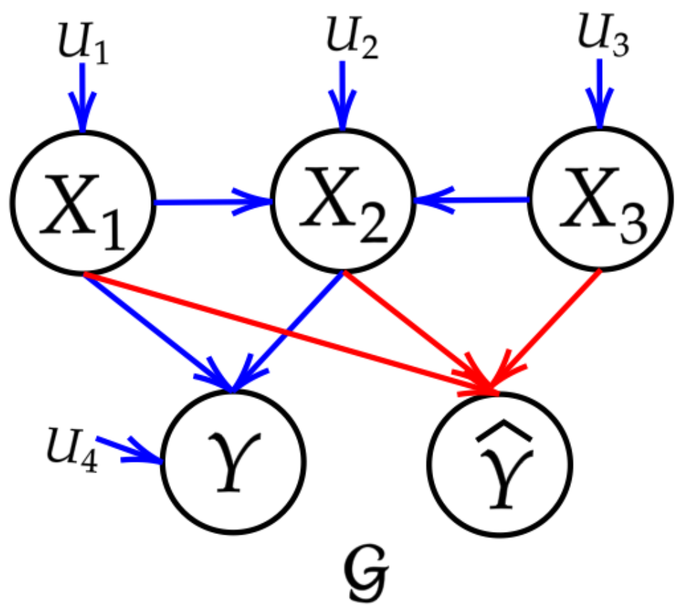
Figure 2: Causal graph $\mathcal{G}$ representing input features $X_{1},X_{2},X_{3}$, true output $Y$ and NN output $\hat{Y}$ (Blue arrows = true causal relationships, Red arrows = relationships learned by traditional NN (without CREDO).

Since neural networks are function approximators (Hornik et al., 1989), for theoretical analysis, w.l.o.g., we marginalize the hidden layers of the NN and show only input and output nodes, similar to (Chattopadhyay et al., 2019; Khademi & Honavar, 2020). Note that $X_{3}$ causes $\hat{Y}$ even though it does not cause the true outcome $Y$, because the NN uses data from all available features. We do not include a noise term for $\hat{Y}$ since it is a deterministic NN function of the inputs.

The graph $\mathcal{G}$ helps us formulate key concepts of this work. We denote the domain prior as the causal relationship between the features $X_{i}$ and true outcome $Y$. While the true relationship is often not known, we assume that properties of the causal effect from features to $Y$ are known to expert users, e.g., a monotonic effect, U-shaped effect, or zero effect of certain features. For example, a user may know that the direct causal effect of $X_{3}$ on $Y$ is zero. In contrast, the relationship learned by the NN corresponds to the edges from features to model prediction $\hat{Y}$ (shown in red in Fig 2). In general, there is no guarantee that the relationship $\hat{Y}=f(X_{1},X_{2},X_{3})$ learned by the NN satisfies the properties given for the true causal effect. The goal of this work is to ensure that the learned relationships in NN aligns with the stated properties of true causal effects.

3.1 Domain Priors

We define a feedforward NN with inputs $X=\{X_{1},X_{2},\dots,X_{d}\}$ as $f:\mathbb{R}^{d}\rightarrow\{1,2,\dots,C\}$ (for classification) or $f:\mathbb{R}^{d}\rightarrow\mathbb{R}$ (for regression). Analogous to the true causal effect of input features on $Y$ ($\mathbb{E}(Y|do(X))$), we define the causal effect of the features on $\hat{Y}$ implied by the NN, $\mathbb{E}(\hat{Y}|do(X))$, as in Kocaoglu et al. (2018); Chattopadhyay et al. (2019). For a given feature $X_{i}$, the ideal goal is to ensure that $\mathbb{E}(\hat{Y}|do(X_{i}))=\mathbb{E}(Y|do(X_{i}))$. In practice, however, a user would not know the true causal effect and instead provide a domain prior on some property satisfied by $\mathbb{E}(Y|do(X))$. Our goal is to ensure that the user-provided property (e.g., monotonicity, $\frac{\partial Y}{\partial do(X_{i})}>0$) is also satisfied by the NN’s learned causal effect $\mathbb{E}(\hat{Y}|do(X))$.

Definition 3.1.

Domain Prior. Given a supervised learning dataset $\{({X}^{j},Y^{j})\}_{j=0}^{n}$, a domain prior for an input feature $X_{i}$ is a property satisfied by its true causal effect on $Y$.

Since the true causal effect (or its properties) cannot be learned from observed data alone, we expect an expert user to provide such priors from domain knowledge. In some cases, the user may also provide the exact domain prior function, $g_{i}^{c}:\mathbb{R}\rightarrow\mathbb{R}$ from the $i^{th}$ input feature to the ground-truth corresponding to the $c^{th}$ output neuron (in regression, there is only one output neuron). If not, given a domain prior shape on $X_{i}$, we provide a simple method to estimate the most likely function satisfying the domain prior on a dataset, under some parametric assumptions (see Sec 4.4 and Appendix for details).

Availability of Domain Priors. Causal domain priors can come in different forms across fields such as algorithmic fairness, economics, health and physical sciences. Specific use cases include: (i) Fairness constraints that require a sensitive attribute’s influence on output to be zero – e.g. skin color in a face classifier (Dash et al., 2022), or race in a loan approval model (Kilbertus et al., 2017); (ii) Monotonic relationship between an input feature and output - e.g., a student’s test score may monotonically affect their admission into a college program, or increasing the number of employees may have a monotonically increasing but diminishing effect on a factory’s productivity (Kahneman & Tversky, 2013); (iii) Arbitrary non-linear functions causally relating input and output - e.g., U-shaped curves have been identified from randomized controlled trials (RCTs) for factors such as cholesterol and diastolic blood pressure (Salkind, 2010) and the dose-response curve for drugs (Calabrese & Baldwin, 2001); or a J-shaped relationship between alcohol and heart disease (Fraser et al., 2016), or Body Mass Index and mortality (Flanders & Augestad, 2008). A more detailed discussion on priors is included in Appendix B.

3.2 Types of Learned Causal Effects in NN

We next define the learned causal effects in an NN model. We consider three kinds of causal effects in this work, as in (Pearl, 2001; VanderWeele, 2011): controlled direct effect, natural direct effect, and (natural) total effect, each of which is defined formally below.

Definition 3.2.

Learned Causal Effect in NN. Given a feedforward NN $f$, the learned causal effect of any feature $X_{i}$ on the NN output $f(X)$ at the end of training is given by $\mathbb{E}(f(X)|do(X_{i}))$.

For convenience, we divide the set of input features $X$ into three disjoint subsets: $T,Z,$ and $W$. $T$ denotes the feature(s) on which we want to enforce a causal domain prior. $Z=\{Z^{1},Z^{2},\dots,Z^{K}\}$ is the set of features that lie on a causal path (in $\mathcal{G}$) between $T$ and $\hat{Y}$ (considering all directed edges, irrespective of color, in Fig 2). $W$ denotes the set of remaining features. Aligning with literature in causality (Pearl, 2009), $T$ is akin to the treatment variable, $\hat{Y}$ is the target variable and $Z^{1},Z^{2},\dots,Z^{K}$ are the mediators. Following Pearl (2009), we use the counterfactual notation $\hat{Y}_{t}(u)$ to denote the value that $\hat{Y}$ would attain under a specific setting of exogenous noise variables $U=u$ and the intervention $do(T=t)$. For the treatment variable $T$, $t^{*}$ denotes the baseline treatment relative to which causal effects are computed. Throughout, we make the following assumption on positivity, common in causal inference (Schwab et al., 2020; Shimizu et al., 2006).

Assumption 3.1.

Positivity. $p(T=t|W,Z)>0$ almost surely for all values of $T$, wherever $p(W,Z)>0$.

Note that we do not need to assume unconfoundedness since it is always satisfied between $\hat{Y}$ and any feature in $\mathcal{G}$. This is because parents of $\hat{Y}$ are the input features, which are all observed. We start by defining the controlled direct effect.

Definition 3.3.

(Controlled Direct Effect in NN). The Controlled Direct Effect ($NN\mathchar 45\relax CDE$) measures the causal effect of treatment $T$ at an intervention $t$ (i.e., $do(T=t)$) on $\hat{Y}$ when all parents of $\hat{Y}$ except $T$ ($Z,W$ in this case) are intervened to pre-defined control values $z,w$ respectively (i.e., $do(Z=z,W=w)$). It is defined as: $NN\mathchar 45\relax CDE^{\hat{Y}}_{t}(z,w,u)\coloneqq\hat{Y}_{t,z,w}(u)-\hat{Y}_{t^{*},z,w}(u)$. Average Controlled Direct Effect ($NN\mathchar 45\relax ACDE$) is defined as: $NN\mathchar 45\relax ACDE^{\hat{Y}}_{t}(z,w)\coloneqq\mathbb{E}_{U}[\hat{Y}_{t,z,w}]-\mathbb{E}_{U}[\hat{Y}_{t^{*},z,w}]=\hat{Y}_{t,z,w}-\hat{Y}_{t^{*},z,w}$.

While the expectation is taken over exogenous noise variables $U$, it can be removed since the neural network $\hat{Y}=f(T,W,Z)$ is a deterministic function which does not depend on the values of the exogenous variables. $t^{*}$ is a baseline treatment value, as stated earlier (we circumvent the need to specify this value in our method, as discussed in Sec 4). The above definition of $NN\mathchar 45\relax ACDE$ is defined for a particular intervention on $\{Z,W\}$ (i.e. all parents of $\hat{Y}$ except $T$) (Pearl, 2001). By our construction, however, the domain priors are expressed only in terms of $T$ and $Y$, so we propose a modified definition for $NN\mathchar 45\relax ACDE$ that marginalizes over $\{Z,W\}$. That is, we take the expectation over $\{Z,W\}$ (average of $NN\mathchar 45\relax ACDE$ for all interventions on $\{Z,W\}$) along with $U$. Our version of $NN\mathchar 45\relax ACDE$ is hence:

$$\begin{split}NN\mathchar 45\relax ACDE^{\hat{Y}}_{t}&\coloneqq\mathbb{E}_{Z,W,U}[\hat{Y}_{t,Z,W}]-\mathbb{E}_{Z,W,U}[\hat{Y}_{t^{*},Z,W}]\\ &=\mathbb{E}_{Z,W}[\hat{Y}_{t,Z,W}]-\mathbb{E}_{Z,W}[\hat{Y}_{t^{*},Z,W}]\end{split}$$

Definition 3.4.

(Natural Direct Effect in NN). The Natural Direct Effect ($NN\mathchar 45\relax NDE$) measures the causal effect of the treatment $T$ at an intervention $t$ (i.e., $do(T=t)$) on $\hat{Y}$ when the nodes of mediating variables $Z$ are intervened to their natural values $Z_{t^{*}}(u)$ (i.e., $do(Z=Z_{t^{*}})$) under baseline treatment $do(T=t^{*})$. $NN\mathchar 45\relax NDE$ is defined as: $NN\mathchar 45\relax NDE^{\hat{Y}}_{t}(u)\coloneqq\hat{Y}_{t,Z_{t^{*}}(u)}(u)-\hat{Y}_{t^{*},Z_{t^{*}}(u)}(u)$. The Average Natural Direct Effect ($NN\mathchar 45\relax ANDE$) is defined as: $NN\mathchar 45\relax ANDE^{\hat{Y}}_{t}\coloneqq\mathbb{E}_{U}[\hat{Y}_{t,Z_{t^{*}}}]-\mathbb{E}_{U}[\hat{Y}_{t^{*},Z_{t^{*}}}]$.

Definition 3.5.

(Total Causal Effect in NN). The Total Causal Effect ($NN\mathchar 45\relax TCE$) of the treatment $T$ at an intervention $t$ (i.e., $do(T=t)$) on $\hat{Y}$ is given by $NN\mathchar 45\relax TCE^{\hat{Y}}_{t}(u)\coloneqq\hat{Y}_{t}(u)-\hat{Y}_{t^{*}}(u)=\hat{Y}_{t,Z_{t}(u)}(u)-\hat{Y}_{t^{*},Z_{t^{*}}(u)}(u)$. The Average Total Causal Effect ($NN\mathchar 45\relax ATCE$) is defined as: $NN\mathchar 45\relax ATCE^{\hat{Y}}_{t}\coloneqq\mathbb{E}_{U}[\hat{Y}_{t,Z_{t}}]-\mathbb{E}_{U}[\hat{Y}_{t^{*},Z_{t^{*}}}]=\mathbb{E}_{U}[\hat{Y}_{t}]-\mathbb{E}_{U}[\hat{Y}_{t^{*}}]$.

For simplicity, in the rest of the paper, we omit the prefix $NN\mathchar 45\relax$ since we always refer to the causal effect in NN when using ACDE, ANDE, ATCE. We use the term Average Causal Effect (ACE) to refer to any of these quantities when the distinction is not necessary.

Types of domain priors considered. Since we consider the aforementioned three kinds of causal effects in NN – controlled direct, natural direct, and (natural) total – accordingly, there are three kinds of domain priors we consider: controlled direct domain prior, natural direct domain prior, and total domain prior. To illustrate, we continue with the BMI example from Sec 1. Consider a drug that decreases a person’s BMI, but which also affects exercise levels. Suppose a randomized trial is conducted to administer the drug and evaluate its effect. Additionally, a free gym membership may be provided to participants of the trial (which would cause people to exercise and thus reduce their BMI). Depending on how the membership was awarded, different kinds of priors may be obtained from the result of the trial. If everyone was provided free gym membership, the result from the trial provides a controlled direct prior; the drug’s direct effect in the population with gym membership is: $\mathbb{E}[Y_{X=1,M=1}]-\mathbb{E}[Y_{X=0,M=1}]$, where $Y$ is BMI, $X$ is whether drug is given and $M$ is whether gym membership is given ($M=1$ to represent the fact that the individual is performing adequate exercise, due to the gym membership). In contrast, if gym membership was awarded only to people who were already exercising, then the trial result will yield a natural direct prior; the effect of the drug at people’s base level of exercise: $\mathbb{E}[Y_{X=1,M_{X=0}}]-\mathbb{E}[Y_{X=0,M_{X=0}}]$. Finally, the total effect measures the entire effect of administering the drug, without influencing exercise habits (which may change because of the effects of the drug).

4 Proposed Method: Identification & Regularization of Causal Effect in NNs

We begin by first proving that the causal effects defined above are identifiable and hence can be regularized in NNs. We then provide our algorithm for regularization, along with a simple method to obtain the domain prior function given its shape (or other properties). The proposed regularizer matches learned causal effect in NN to the domain prior function, as defined in Sec 3.1.

Matching gradients. Given a domain prior function $g_{i}^{c}$, our objective is to ensure that the causal effects learned by the NN match the prior. Instead of directly matching causal effects, we rather match the gradient of NN’s causal effect with the gradient of $g_{i}^{c}$ for three reasons: (i) Properties of prior causal knowledge expressed as a shape (or relative values) is common in many applications, making gradient matching more natural (and avoiding errors in specification of absolute values/constant terms); (ii) There is no closed form expression for the interventional expectation terms (Defns 3.3-3.5), thus making gradient matching more computationally efficient; and (iii) gradient matching avoids having to choose a particular baseline treatment value. We hence match the gradient of $g_{i}^{c}$ with the gradient of ACE of the $i^{th}$ input feature on $\hat{Y}$ under the graph $\mathcal{G}$ (as in Fig 1). For each of the causal effects considered – controlled direct, natural direct and total, we now show that the effect is identifiable in NNs and then provide regularization procedures.

4.1 Identifying and Regularizing ACDE

Given an NN $f$, a datapoint $(t,z,w)\sim(T,Z,W)$ and its prediction $f(t,z,w)$ (we also use $\hat{Y}(t,z,w)$ to refer to the same quantity), we can intervene on $T$ with $t^{\prime}$ and compute $f(t^{\prime},z,w)$. $f(t^{\prime},z,w)-f(t,z,w)$ then gives an intuitive expression for the direct effect of $T$ on output. Below we show that this formula captures CDE as in Defn 3.3.

Proposition 4.1 (ACDE Identifiability in Neural Networks).

For a neural network with output $\hat{Y}$, the ACDE of a feature $T$ at $t$ on $\hat{Y}$ is identifiable and given by $ACDE^{\hat{Y}}_{t}=\mathbb{E}_{Z,W}\big{[}\hat{Y}|t,Z,W\big{]}-\mathbb{E}_{Z,W}\big{[}\hat{Y}|t^{*},Z,W\big{]}$.

Proofs of all propositions are in the Appendix for convenience of reading. Since the ACDE is measured as the change in interventional expectation w.r.t. a baseline, the expected gradient of $\hat{Y}$ w.r.t. $t$ at $(t,z,w)$ is equivalent to the gradient of ACDE w.r.t. $t$.

Proposition 4.2 (ACDE Regularization in Neural Networks).

The $n^{th}$ partial derivative of $ACDE$ of $T$ at $t$ on $\hat{Y}$ is equal to the expected value of $n^{th}$ partial derivative of $\hat{Y}$ w.r.t. $T$ at $t$, that is: $\frac{\partial^{n}ACDE^{\hat{Y}}_{t}}{\partial t^{n}}=\mathbb{E}_{Z,W}\big{[}\frac{\partial^{n}[\hat{Y}(t,Z,W)]}{\partial t^{n}}\big{]}$.

Propn 4.2 allows us to enforce causal priors in an NN model by matching gradients. For an NN model with $d$ inputs and $C$ outputs, let $x^{j}$ (instance of random variable $X$) denote the $j^{th}d$-dimensional input to the NN. For a given data point $x^{j}$, let $\delta G^{j}$ represent the matrix (of dimension $C\times d$) of derivatives of all available priors $g^{i}_{c}$ w.r.t. $x^{j}$, i.e. $\delta G_{c,i}^{j}$ denotes the derivative of function $g_{i}^{c}$ w.r.t. $i^{th}$ feature of $x^{j}$. To enforce $f$ to maintain known prior causal knowledge (in terms of gradients), we define our regularizer $R$ as:

$$R(f,G,M)=\frac{1}{N}\sum_{j=1}^{N}\max\{0,\|\nabla_{j}f\odot M-\delta G^{j}\|_{1}-\epsilon\}$$ (1)

where $\nabla_{j}f$ is the $C\times d$ Jacobian of $f$ w.r.t. $x^{j}$; $M$ is a $C\times d$ binary matrix that acts as an indicator of features for which prior knowledge is available; $\odot$ represents the element-wise (Hadamard) product; $N$ is the size of training data; and $\epsilon$ is a hyperparameter to allow a margin of error. For the case where we wish to make gradient of ACDE of a feature to be zero, we set $M_{c,i}=1$ and $\delta G_{c,i}$ to be $0$ and the regularizer hence simplifies into: $R(f,G,M)=\frac{1}{N}\sum_{j=1}^{N}\max\{0,\|\nabla_{j}f\odot M\|_{1}-\epsilon\}$, which is equivalent to the loss function defined in fairness literature (Ross et al., 2017; Gupta et al., 2019).

4.2 Identifying and Regularizing ANDE

To identify natural effects in NNs, we need to know: (i) which features belong to the mediating variables set $Z$ (enough to know the partial causal graph containing $Z$); and (ii) the structural equations of how $Z$ changes when $T$ changes (Defns 3.4 & 3.5). (If we do not know which nodes belong to $Z$, it is not possible to learn them from training data because there exists a set of causal graphs that are Markov-equivalent w.r.t. a given training distribution, each leading to different causal effects (Pearl, 2009), making this non-identifiable.) When $Z$ is an empty set, ACDE obtained by controlling for $W$ is equivalent to ANDE (Zhang & Bareinboim, 2018). When $Z$ is known (i.e., mediating variables and their structure) and is non-empty, we now show that we can identify and regularize ANDE in $f$ w.r.t. a baseline treatment value $t^{*}$, under the below assumption.

Assumption 4.1.

(Unconfoundedness of T and Z). $\mathcal{G}$ contains no unobserved confounders betweeen input features subset $T$ and its mediators $Z$ wrt. $\hat{Y}$, i.e. observed features block all backdoor paths between $T$ and $Z$.

Proposition 4.3 (ANDE Identifiability in Neural Networks).

Under Assumption 4.1, the ANDE of $T$ at $t$ on $\hat{Y}$ is identifiable and is given by $ANDE^{\hat{Y}}_{t}=\mathbb{E}_{Z_{t^{*}},W}[\hat{Y}|t,Z_{t^{*}},W]-\mathbb{E}_{Z_{t^{*}},W}[\hat{Y}|t^{*},Z_{t^{*}},W]$.

Proposition 4.4 (ANDE Regularization in Neural Networks).

The $n^{th}$ partial derivative of $ANDE$ of $T$ at $t$ on $\hat{Y}$ is equal to the expected value of $n^{th}$ partial derivative of $\hat{Y}$ w.r.t. $T$ at $t$ , that is, $\frac{\partial^{n}ANDE^{\hat{Y}}_{t}}{\partial t^{n}}=\mathbb{E}_{Z_{t^{*}},W}\big{[}\frac{\partial^{n}[\hat{Y}(t,Z_{t^{*}},W)]}{\partial t^{n}}\big{]}$.

In this case, R($f$,G,M) is the same as Eqn 1 with the only difference that $\nabla_{j}f$ is evaluated at $(t,Z_{t^{*}},W)$.

4.3 Identifying and Regularizing ATCE

Given known $Z$, similar to ANDE, the ATCE of $T$ at $t$ on $\hat{Y}$ is identifiable under assumptions similar to the previous case, as shown below.

Proposition 4.5 (ATCE Identifiability in Neural Networks).

Under Assumption 4.1, the total causal effect of $T$ at $t$ on $\hat{Y}$ is identifiable and is given by $ATCE^{\hat{Y}}_{t}=\mathbb{E}_{Z_{t},W}[\hat{Y}|t,Z_{t},W]-\mathbb{E}_{Z_{t^{*}},W}[\hat{Y}|t^{*},Z_{t^{*}},W]$.

Proposition 4.6 (ATCE Regularization in Neural Networks).

The gradient of the Average Total Causal Effect (ATCE) of $T$ at $t$ on $\hat{Y}$ is equal to the expected value of the total gradient of $\hat{Y}$ w.r.t. $T$ at $t$, that is, $\frac{dATCE^{\hat{Y}}_{t}}{dt}=\mathbb{E}_{Z_{t},W}\big{[}\frac{d[\hat{Y}(t,Z_{t},W)}{dt}\big{]}$.

To regularize the total causal effect, we match the total derivative of $\hat{Y}$ w.r.t. $t$ with the gradient of a given total causal effect prior. The regularizer $R(f,G,M)$ that enforces a NN model to maintain known total causal effect is then:

$$R(f,G,M)=\frac{1}{N}\sum_{j=1}^{N}\max\{0,\|\nabla_{j}^{t}f\odot M-\delta G^{j}\|_{1}-\epsilon\}$$ (2)

where $\nabla_{j}^{t}f$ is the $C\times d$ matrix of total derivatives at input $x^{j}$. The computation of the total derivative is described in Algorithm 1. Other variables are as defined in Eqn. 1.

4.4 Final Algorithm: CREDO

To summarize, the overall optimization problem with the proposed CREDO regularizer to train the NN is given by:

$$\arg\min_{\theta}ERM+\lambda_{1}R(f,G,M)$$ (3)

where $\theta$ are parameters of the NN $f$, $ERM$ stands for traditional Empirical Risk Minimizer over the given dataset (based on loss functions such as cross-entropy loss). The regularizer $R(f,G,M)$ is defined differently for each desired causal effect and is summarized in Algorithm 1.

Result: Regularizers for ACDE, ANDE, ATCE in $f$.

Input: $\mathcal{D}=\{(x^{j},y^{j})\}_{j=1}^{N}$, $y^{j}\in\{0,1,\dots,C\}$, $x^{j}\sim X^{j}$; $\mathbb{Q}=\{i|\exists\ g^{c}_{i}\ for\ some\ c\}$; $\mathbb{G}=\{g_{i}^{c}|g_{i}^{c}$ is prior for $i^{th}$ feature w.r.t. class c}; $\mathbb{F}=\{f^{1},\dots,f^{K}\}$ is the set of structural equations of the underlying causal model s.t $f^{i}$ describes $Z^{i}$; $\epsilon$ is a hyperparameter

Initialize: $j=1,\delta G^{j}=\vmathbb{0}_{c\times d}\forall j=1,...,N$, $M=\vmathbb{0}_{c\times d}$

while $j\leq N$ do

       foreach $i\in\mathbb{Q}$ do

             foreach $g_{i}^{c}\in\mathbb{G}$ do

                   $\delta G^{j}[c,i]=\nabla g_{i}^{c}\big{|}_{x_{i}^{j}}$; $M[c,i]=1$ case 1: regularizing ACDE do

                         $\nabla_{j}f[c,i]=\frac{\partial\hat{Y}}{\partial x_{i}}\rvert_{x^{j}}$

                   case 2: regularizing ANDE do

                         /* causal graph is known */ $t=x_{i}$
$\nabla_{j}f[c,i]=\frac{\partial\hat{Y}}{\partial x_{i}}\rvert_{(t^{j},z_{t^{*}}^{j},w^{j})}$

                   case 3: regularizing ATCE do

                         /* causal graph is known */ $\nabla_{j}f[c,i]=\left[\frac{d\hat{Y}}{dx_{i}}+\sum_{l=1}^{K}\frac{\partial\hat{Y}}{\partial Z^{l}}\frac{df^{l}}{dx_{i}}\right]\rvert_{x^{j}}$

                  

             end foreach

            

       end foreach

      $j=j+1$

end while

return $\frac{1}{N}\sum_{j=1}^{N}max\{0,\lVert{\nabla_{j}f\odot M-\delta G^{j}\rVert}_{1}-\epsilon\}$

Algorithm 1 CREDO Regularizer

Inferring domain prior function. When a user provides the domain prior as a shape (not the exact function), we assume a parametric form (see Table 1 for examples) for the prior function and select the parameters for which we obtain best validation accuracy. Typically, expert users may be able to specify the search space for a prior (e.g., linear, quadratic in a range); if not, we assume the simplest parametric form satisfying the prior shape. We provide a detailed discussion and present this hyperparameter search in Appendix C.2. We note that this work assumes that the prior comes from a domain expert and is hence correct – validating the prior’s correctness may be an independent future direction by itself.

Domain	Example Prior	Functional form
Fairness	Zero causal	$\hat{Y}_{t}=\alpha;\forall\alpha$
(Dash et al. 2021)(Berk 2019)	effect
Healthcare	U-shape of	$\hat{Y}_{t}=at^{2}$
(Calabrese et al. 2001)(Salkind 2010)	drug effect
Healthcare	J-shape of BMI	$\hat{Y}_{t}=ae^{bt^{2}};x>0$
(Flanders et al. 2008)(Fraser et al. 2016)	on mortality
Economics	Diminishing	$\hat{Y}_{t}=-at^{3}+bt^{2}$
(Kahneman et al. 2013)(Brue 1993)	returns

Table 1: Examples of availability of domain priors ($a,b\in\mathbb{R}^{+}$).

5 Experiments and Results

We conducted a comprehensive suite of experiments on real-world and synthetic datasets with different kinds of domain priors to study the proposed method. Our goal was to evaluate whether models trained with CREDO exhibit the correct causal effect as specified by the domain prior. We also show that the models trained by CREDO get better test set performance on noisy input data.

Datasets and Priors. We use two kinds of datasets: 1) Four benchmark synthetic datasets from the BNLearn repository (Scutari & Denis, 2014) where the causal graph is known and all effects can be computed; and 2) Eight real-world datasets without knowledge of true causal graph where only $ACDE$ can be computed. BNLearn datasets are Bayesian networks generated from conditional linear Gaussian mechanisms, so the ground-truth domain priors are derived from the generating equations. For the real-world datasets, prior shapes are derived from domain knowledge. E.g., in the Boston Housing dataset, we use a ground-truth prior that number of rooms should have an increasing monotonic effect on the price of a house. Details of the 12 datasets and known causal graphs are in the Appendix.

Evaluation Metrics. Ideally, we would like to compare the error between $E[\hat{Y}|do(X=x)]$ for an NN model and the domain prior for different values of $X$, but there are two challenges. Firstly, the domain prior is not an exact function but a shape provided by user, except when effect is zero. For non-zero effect priors, if the dataset is synthetic, we assume that domain function prior is the true SCM equation for connecting $X$ and $Y$ (CREDO does not have access to the SCM equations). For real-world datasets, we choose the function that provides best accuracy on a held-out validation dataset, using the hyperparameter search procedure described in Appendix. Secondly, it is non-trivial to estimate ATCE, $E[\hat{Y}|do(X_{i}=x)]$ since the identified backdoor estimand, $E[\hat{Y}|do(X_{i}=x)]=\sum_{w}E[\hat{Y}|X_{i}=x,W=w]P(W=w)$ requires a sum over all values of other features; ACDE and ANDE have similar expressions. Therefore, we use the method from Chattopadhyay et al. (2019) to estimate ATCE, ACDE and ANDE for an NN model. It outputs the causal effect at each value of $X_{i}$, thus yielding an ACE curve. A description of this method is in Appendix for completeness. Given a domain prior function and an ACE estimate of a trained NN, we consider the following metrics to compare them: Root Mean Square Error (RMSE), Frechet score and Pearson correlation coefficient. We also report test accuracies to confirm that our regularizer maintains test set performance while incorporating causal priors.

Baselines. We compare against vanilla Empirical Risk Minimization (ERM) without our regularizer in all our experiments. In a setting of making ACDE zero, our method becomes the same as (Ross et al., 2017) and one would obtain the same results; hence we do not compare explicitly. In a setting of making ACDE match a monotonic prior, we compare with Point Wise Loss (PWL) (Gupta et al., 2019) and Deep Lattice Networks (DLN) (You et al., 2017). In all results, “GT” (prefixed with the variable) refers to the ground-truth prior provided.

Our code is made available for reproducibility. Other experimental details including $Z_{t}$ estimation, NN architectures and training hyperparameters are in Appendix C, G & H.

5.1 Synthetic Data With Linear or Zero Domain Priors

SANGIOVESE:

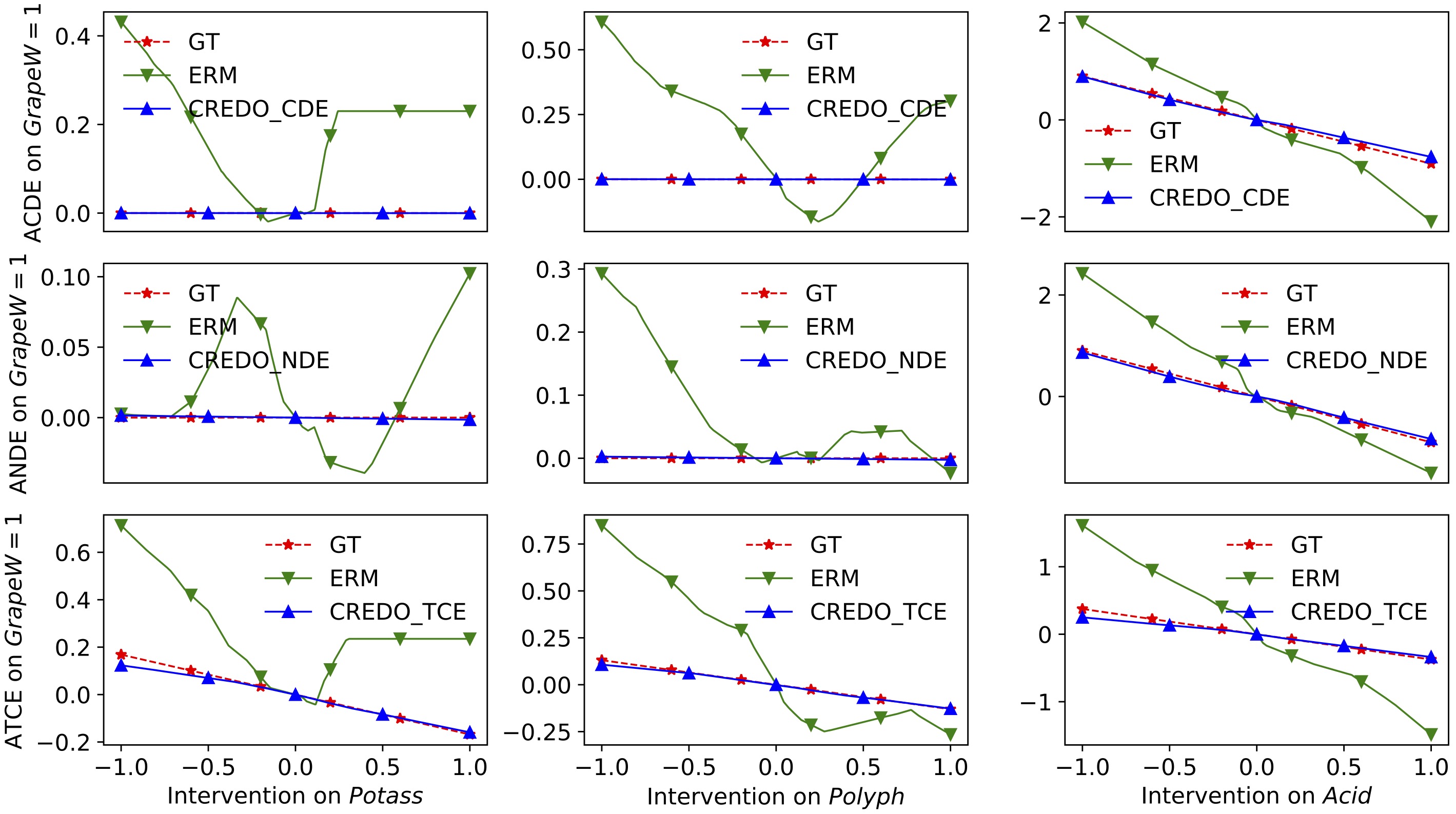
Figure 3: Results on SANGIOVESE: Comparison of ACDE, ANDE, ATCE learned by ERM and CREDO models.

We generate data from the SANGIOVESE conditional linear Gaussian Bayesian network. We consider the output (“GrapesYield”) as a categorical variable and train an NN that predicts if the yield of grapes is better than average. Based on the causal graph and GrapesYield’s true structural equation, we choose two kinds of priors: 1) DirectParentPrior: a linear decreasing ATCE, ANDE and ACDE of Acid feature on output (all three effects are the same since Acid is a parent of GrapesYield); and 2) AncestorPrior: zero ACDE and ANDE for Potass (potassium content) and Polyph (total polyphenolic content) on output while having a small, non-zero total effect, ATCE. Fig 3 shows ACE plots and ground-truth ACE for ERM and CREDO. Evidently, CREDO helps conform to the given causal prior for all three features (red and blue lines coincide for ATCE, ANDE and ACDE) whereas ERM model obeys monotonicity only for the Acid feature. The quantitative metrics in Table 2 further show the benefit of CREDO regularization. RMSE and Frechet distance are both substantially lower for CREDO than ERM: more than 100 times lower for Potass and Polyph features, and 16-33% lower for Acid feature. CREDO matches the prior without a substantial drop in accuracy. Our results on MEHRA, SACHS and Asia datasets from the BNLearn repository showed similar trends, and are reported in the Appendix.

Feature	RMSE		Frechet		Corr
	ERM	CREDO	ERM	CREDO	ERM	CREDO
ACDE ($\lambda_{1}=1.4$) - (Test Acc:ERM: 82.95%, CREDO: 82.60%)
Potass	0.216	0.000	0.431	0.000	-	-
Polyph	0.273	0.000	0.607	0.000	-	-
Acid	0.600	0.064	2.096	0.894	0.997	0.998
ANDE ($\lambda_{1}=1.0$) - (Test Acc:ERM: 82.95%, CREDO: 82.75%)
Potass	0.043	0.000	0.102	0.001	-	-
Polyph	0.111	0.001	0.293	0.002	-	-
Acid	0.684	0.046	2.425	0.866	0.993	0.999
ATCE ($\lambda_{1}=1.5$) - (Test Acc:ERM: 82.95%, CREDO: 82.10%)
Potass	0.303	0.016	0.714	0.159	0.547	0.997
Polyph	0.325	0.008	0.849	0.128	0.937	0.998
Acid	0.423	0.025	1.059	0.208	0.547	0.996

Table 2: Results on SANGIOVESE

5.2 Synthetic Data With Non-Linear Domain Priors

For a fair comparison to PWL and DLN, we consider two synthetic datasets motivated from their paper. These datasets have non-linear monotonic relationships in the true structural equations, and we hence input a non-linear prior to CREDO. These datasets have the form $z=\log(1+2x),x\in[0,1]$ and $z=\sin(x)+e^{y}$, $x\in[0,1]$, $y\in[0,1]$. The domain priors provided by a user is a log-linear monotonic relationship of $x$ to output $z$ for $z=\log(1+2x),x\in[0,1]$ and $z$ is monotonically increasing w.r.t. $y$ when $x$ is kept constant for $z=\sin(x)+e^{y}$, $x\in[0,1]$, $y\in[0,1]$. CREDO uses the shape of the prior while PWL and DLN can only regularize for monotonic constraints. As a result, we observe that CREDO matches the prior shape better when compared to PWL and DLN (Fig 4). In particular, using DLN is worse than using ERM as the DLN model exaggerates the ACDE substantially (has higher RMSE and Frechet Score). In addition, there is no benefit in using PWL over ERM; both are almost identical in their ACDE. CREDO model is the closest to the ground-truth prior.

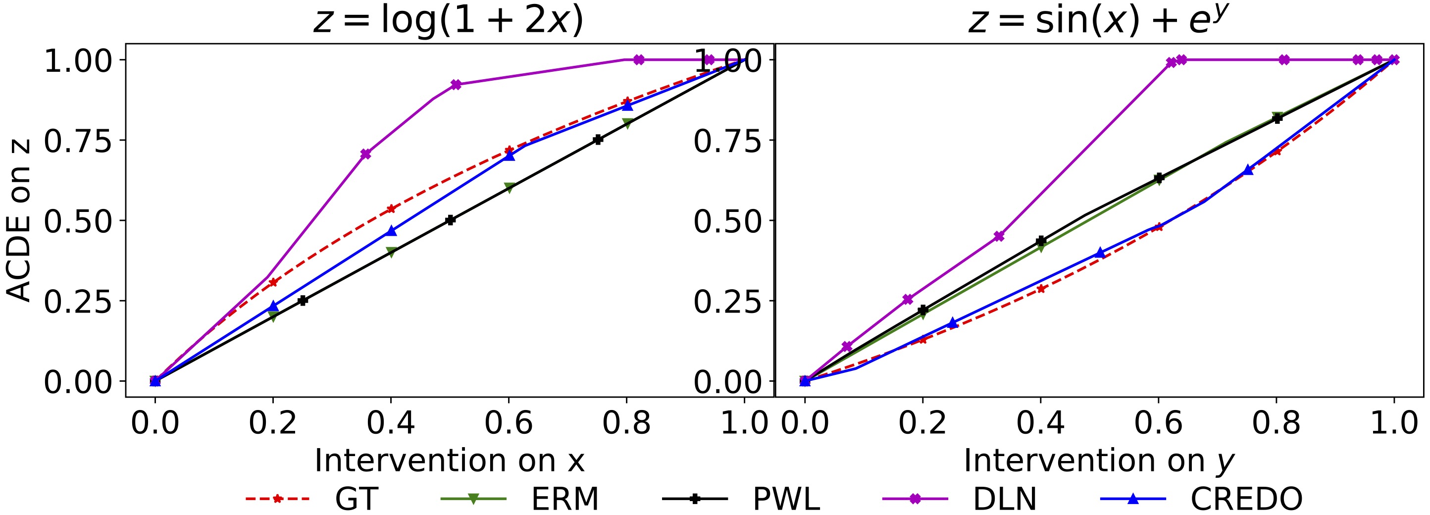
Figure 4: Enforcing monotonicity. ACDE plots of ERM, CREDO, PWL and DLN on Synthetic Tabular datasets. CREDO matches GT better than other methods.

5.3 When Causal Graph is Unknown

As stated in Sec 4, when we do not know the causal graph, the best we can do is regularize for ACDE. Below, we apply CREDO on real-world datasets for regularizing ACDE of an NN. In such cases, we expect a domain expert to provide prior function properties such as shape and/or a search space for its parameters. As stated earlier (and described in the Appendix), we find the best parameters for the prior function by tuning for highest validation-set accuracy.

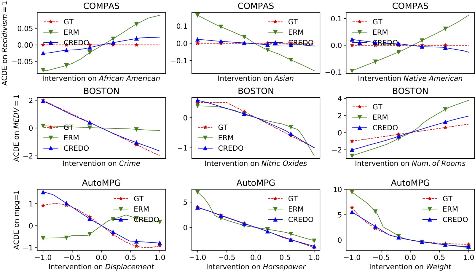
Figure 5: Results on COMPAS, BOSTON, and AutoMPG datasets

COMPAS: The task herein (Angwin et al., 2016) is to predict the likelihood of two-year recidivism (re-offending in next two years) given a set of features (Berk et al., 2021; Berk, 2019; Brennan & Oliver, 2013; Ferguson, 2014). From a fairness perspective, we expect NN models to have zero direct causal effect of race while predicting recidivism (Pearl, 2009). Table 3 and Fig 5 shows our results. CREDO is able to align ACDE of race on two-year recidivism prediction to be close to zero with almost the same model accuracy. Note the significant reduction in RMSE and Frechet scores, which measure the alignment of the trained NN’s ACE w.r.t. the domain prior.

AutoMPG: The AutoMPG dataset contains the mileage of various cars given attributes such as weight, horsepower, displacement, etc (Dua & Graff, 2017). We learn an NN classifier that can predict if the mileage is better than average. We want displacement, weight and horsepower to have a decreasing causal effect w.r.t. mileage. Results shown in Table 3 and Fig 5 once again support the usefulness of our method.

Boston Housing: This dataset concerns home values in the suburbs of Boston (Dua & Graff, 2017). We convert the output attribute home value into a categorical output, and learn a classifier that can predict if the home value is better than average. As the domain prior, we want crime rate and concentration of Nitric Oxides (above a threshold) to have a decreasing causal effect and number of rooms (RM) to have an increasing causal effect w.r.t. housing prices. Results in Table 3 and Fig 5 show that CREDO helps align the ACDE of the trained model with the prior in all these cases.

Feature	RMSE		Frechet Score		Corr. Coeff.
	ERM	CREDO	ERM	CREDO	ERM	CREDO
COMPAS ($\lambda_{1}=5$) (ERM test accuracy is 67.90%, CREDO test accuracy is 67.09%)
African American	0.055	0.016	0.088	0.025	-	-
Asian	0.092	0.018	0.162	0.021	-	-
Native American	0.059	0.011	0.109	0.025	-	-
AutoMPG ($\lambda_{1}=1.5$) (ERM test accuracy is 88.6%, CREDO test accuracy is 87.34%)
Displacement	1.144	0.212	0.566	1.524	-0.945	0.977
Horsepower	1.036	0.081	6.978	3.908	0.922	0.999
Weight	1.780	0.25	9.453	5.510	0.986	0.992
Boston ($\lambda_{1}=2.2$) (ERM test accuracy is 88.2%, CREDO test accuracy is 85.30%)
Crime	0.52	0.145	0.181	1.951	0.996	0.999
Nitric Oxide	0.165	0.080	1.265	0.994	0.957	0.991
Num. of Rooms	0.994	0.036	3.786	2.009	0.993	1.000

Table 3: Enforcing Causal Effects (ACDE) of Multiple Variables: Results on COMPAS, AutoMPG, and BOSTON datasets

We obtain similar results on enforcing domain priors over the MEPS, Law School Admission, Adult, Car Evaluation, and Titanic datasets, as shown in the Appendix.

5.4 Robustness to Noisy Input

We study the robustness of CREDO models when the test data is noisy. For SANGIOVESE and AutoMPG (classification datasets), we perturb test samples by adding zero-mean Gaussian noise. For synthetic tabular (regression) datasets, we study robustness to out-of-domain test samples (the domains are given in section 5.2). As in Table 4, CREDO models, which are trained to respect true causal relationships, are more robust to test-time perturbations (especially with higher noise variance) for both classification and regression datasets.

	Variance 0.2		Variance 0.5		Variance 1.0
Dataset	ERM	CREDO	ERM	CREDO	ERM	CREDO
SANGIOVESE	73.15	73.95	61.60	63.20	55.45	56.00
AutoMPG	86.07	84.80	79.74	83.54	68.35	79.74
Dataset	ERM			CREDO
$z=\log(1+2x),x\in[1,2]$	0.094			0.073
$z=\sin(x)+e^{y}$, $x\in[0,1]$, $y\in[1,2]$	21.75			20.29

Table 4: Robustness results: Accuracy on noisy test data and MSE on out-of-distribution samples of ERM, CREDO models

5.5 Relation to Fairness

Regularizing ACDE can be viewed as being close to achieving no proxy discrimination in expectation: $\mathbb{E}(\hat{Y}|do(T=t))=\mathbb{E}(\hat{Y}|do(T=t^{\prime}))$ (Kilbertus et al., 2017) in fairness applications. That is, NN output $\hat{Y}$ should not depend on the intervention on $T$ when making predictions. To encourage fairness, we enforce the ACDE of protected attributes on the outcome to be zero so that all interventions to the treatment variable $T$ lead to the same outcome, zero in this case. Results shown in the Table 5 demonstrate that CREDO outperforms ERM on various datasets w.r.t. the fairness metric: Disparate Impact (higher is better) which captures the property of no proxy discrimination in expectation through the ratio $\frac{p(\hat{Y}=1|do(T=t))}{p(\hat{Y}=1|do(T=t^{\prime}))}$. Where $\hat{Y}=1$ signifies positive outcome, $t$ denotes the unprivileged group, and $t^{\prime}$ denotes the privileged group.

Datasets ($\rightarrow$)	Law School		MEPS	COMPAS
Model ($\downarrow$)	Gender	Race	Race	African American	Asian	Native American
ERM	0.94	0.91	0.77	0.82	0.95	0.63
CREDO	0.99	0.94	0.84	0.83	0.84	0.82

Table 5: ERM vs CREDO on Disparate Impact metric

We also compared CREDO with two standard fair classification algorithms: Exponentiated Gradient (EG) and Grid Search (GS) (Agarwal et al., 2018)(we use the code from https://fairlearn.org to implement these algorithms) on the Boston Housing dataset (Table 6). Along with ACDE, we use a fairness-based metric: Demographic Parity Difference (Lower is better). We enforced a constraint that ACDE of sensitive features: proportion of black people (B) and % of lower status of population (LSTAT) should be zero on house price prediction.

Model	ACDE	ACDE	Demog	Test
	(B)	(LSTAT)	Par Diff	Accuracy
ERM	0.10	0.39	0.86	88.23%
EG	0.18	0.33	0.45	77.50%
GS	0.08	0.33	0.79	86.50%
CREDO	0.00	0.23	0.66	86.27%

Table 6: CREDO vs fair classifiers

Results show that CREDO performs on par w.r.t. fairness metric and better w.r.t. ACDE metric, which captures causal attribution.

Results on more datasets are in Appendix D. Ablation studies, effect of regularization co-efficient, time complexity, and discussion on incorrect priors are in Appendix E.

6 Conclusion

In this work, we propose a new causal regularization method, CREDO, that can learn neural network models whose learned causal effects match prior domain knowledge as provided by an expert user. We show that the method can work with any differentiable prior representing complete or partial understanding of the domain. Importantly, we distinguish between direct and total causal effects, and show how both can be considered in CREDO. We performed extensive experiments on various datasets, with known and unknown causal graphs, and with different kinds of priors. CREDO shows promising performance in matching causal domain priors while maintaining test accuracy.

Appendix

In this appendix, we include the following information.

• Proofs of propositions in Section A

• Discussion on sources of causal domain priors for using CREDO in practice in Section B

• Implementation details of CREDO in Section C

• More experimental results in Section D

  • Experiments on BNLearn datasets

  • Enforcing fairness constraints

• Ablation studies and analysis in Section  E

• Description of computation of ACE (Average Causal Effect), as in (Chattopadhyay et al., 2019) in Section F

• Causal graphs/DAGs for BNLearn datasets in Section G

• Architectures/training details of our models for all datasets in Section H

Appendix A Proofs of Propositions

We begin writing the proofs of our propositions by recollecting two key results from (Pearl, 2009) which we use in our proofs: (i) When there is no backdoor path from treatment $T$ to the outcome $\hat{Y}$, interventional distribution is equal to the conditional distribution i.e., $p(\hat{Y}|do(T=t))=p(\hat{Y}_{t})=p(\hat{Y}|T=t)$. (ii) If there exist a set of nodes $W$ that satisfy the backdoor criteria relative to the causal effect of $T$ on $\hat{Y}$, the causal effect of $T$ on $\hat{Y}$ can be evaluated using the adjustment formula $\mathbb{E}[\hat{Y}_{t}]=\mathbb{E}[\hat{Y}|do(T=t)]=\sum_{\hat{Y}}\hat{Y}p(\hat{Y}|do(T=t))=\sum_{w}\sum_{\hat{Y}}\hat{Y}p(\hat{Y}|T=t,W=w)p(W=w)$. Note that this is equivalent to $\mathbb{E}_{W}[\hat{Y}|t,W]$ in our notation, since the inner expectation over $\hat{Y}$ vanishes due to the deterministic nature of the NN. See 4.1

Proof.

Starting with the definition of $ACDE$ of $T$ at $t$ on $\hat{Y}$ (Equation 1 of main paper), we get

$$ACDE^{\hat{Y}}_{t} =\mathbb{E}_{{Z,W,U}}[\hat{Y}_{t,{Z,W}}]-\mathbb{E}_{{Z,W,U}}[\hat{Y}_{t^{*},{Z,W}}]]$$

$$=\mathbb{E}_{Z,W}[\hat{Y}_{t,{Z,W}}]-\mathbb{E}_{Z,W}[\hat{Y}_{t^{*},{Z,W}}\big{]}$$

$$=\mathbb{E}_{Z,W}[\hat{Y}|t,{Z,W}]-\mathbb{E}_{Z,W}[\hat{Y}|t^{*},{Z,W}\big{]}$$

Since a NN $f$ is a deterministic function of its inputs, expectation over $U$ can be discarded once we condition on all features (second equality above). Further, once all parents of $\hat{Y}$ (i.e., $T,Z,W$) are intervened, there cannot be an unobserved confounder that causes both $\hat{Y}$ and $T$. Hence unconfoundedness is valid for the effect from $T$ to $\hat{Y}$. For this reason, we can replace the intervention with conditioning in the last step. ∎

See 4.2

Proof.

Using the identifiability result from Proposition 4.1,

$$ACDE^{\hat{Y}}_{t}=\mathbb{E}_{{Z,W}}\big{[}\hat{Y}|t,{Z,W}\big{]}-\mathbb{E}_{{Z,W}}\big{[}\hat{Y}|t^{*},{Z,W}]\big{]}$$

Now, taking the $n^{th}$ partial derivative w.r.t $t$ on both sides,

$$\frac{\partial^{n}ACDE^{\hat{Y}}_{t}}{\partial t^{n}} =\frac{\partial^{n}[\mathbb{E}_{{Z,W}}[\hat{Y}|t,{Z,W}]-\mathbb{E}_{{Z,W}}[\hat{Y}|t^{*},{Z,W}]]}{\partial t^{n}}$$

$$=\frac{\partial^{n}[\mathbb{E}_{{Z,W}}[\hat{Y}|t,{Z,W}]]}{\partial t^{n}}(\because t^{*}\ is\ a\ constant)$$

$$=\mathbb{E}_{{Z,W}}\left[\frac{\partial^{n}[\hat{Y}({t,{Z,W}})]}{\partial t^{n}}\right]$$

Note the change in notation in last step ($\hat{Y}({t,{Z,W}})$ vs $\hat{Y}|{t,{Z,W}}$). This change is merely to differentiate between conditioning (when taking expectation) and evaluating (when taking partial derivative). However both quantities are the same. ∎

See 4.3

Proof.

Assuming that the set $W$ forms a valid adjustment set in the calculation of causal effect of $T$ on $\hat{Y}$, from the backdoor adjustment formula (Pearl, 2009), we get $\mathbb{E}_{U}[\hat{Y}_{t,Z_{t^{*}}}]=\mathbb{E}_{W,U}[\hat{Y}_{t,Z_{t^{*}}}|W]$. However, the value $Z_{t^{*}}$ not only depends on the intervention $do(T=t^{*})$ but also on $U,W$. That is, $Z_{t^{*}}$ is a random variable which is a function of $W,U$. So, $\mathbb{E}_{W,U}[\hat{Y}_{t,Z_{t^{*}}}|W]$ can be written as (Pearl, 2001):

$$\mathbb{E}_{W,U}[\hat{Y}_{t,Z_{t^{*}}}|W]=\mathbb{E}_{W,U}\sum_{Z_{t^{*}}}[\hat{Y}_{t,Z_{t^{*}}}|Z_{t^{*}},W]p(Z_{t^{*}}|W)$$

Using consistency (Pearl, 2009) and backdoor adjustment, we have: $\mathbb{E}_{U}[\hat{Y}_{t,Z_{t^{*}}}]=\mathbb{E}_{Z_{t^{*}},W,U}[\hat{Y}|{t,Z_{t^{*}},W}]$.

$$ANDE^{\hat{Y}}_{t} =\mathbb{E}_{U}[\hat{Y}_{t,Z_{t^{*}}}]-\mathbb{E}_{U}[\hat{Y}_{t^{*},Z_{t^{*}}}]$$

$$=\mathbb{E}_{Z_{t^{*}},W,U}[\hat{Y}|t,Z_{t^{*}},W]-\mathbb{E}_{Z_{t^{*}},W,U}[\hat{Y}|t^{*},Z_{t^{*}},W]]$$

$$=\mathbb{E}_{Z_{t^{*}},W}[\hat{Y}|t,Z_{t^{*}},W]-\mathbb{E}_{Z_{t^{*}},W}[\hat{Y}|t^{*},Z_{t^{*}},W]$$

The second equality is because of the adjustment formula as described above. Further, similar to the ACDE case, the third equality is because once we condition on all input features, $f$ is a deterministic function of its inputs and hence expectation over noise variables can be omitted. Further, $Z_{t^{*}}$ is identified because all parents of Z are observed as per Assumption 1. ∎

See 4.4

Proof.

Using the identifiability result from Proposition 4.3,

$$ANDE^{\hat{Y}}_{t}=\mathbb{E}_{Z_{t^{*}},W}[\hat{Y}|t,Z_{t^{*}},W]-\mathbb{E}_{Z_{t^{*}},W}[\hat{Y}|t^{*},Z_{t^{*}},W]$$

Now, taking the $n^{th}$ partial derivative w.r.t $t$ on both sides,

$$\frac{\partial^{n}ANDE^{\hat{Y}}_{t}}{\partial t^{n}} =\frac{\partial^{n}\big{[}\mathbb{E}_{Z_{t^{*}},W}[\hat{Y}|t,Z_{t^{*}},W]-\mathbb{E}_{Z_{t^{*}},W}[\hat{Y}|t^{*},Z_{t^{*}},W]\big{]}}{\partial t^{n}}$$

$$=\frac{\partial^{n}\big{[}\mathbb{E}_{Z_{t^{*}},W}[\hat{Y}|t,Z_{t^{*}},W]\big{]}}{\partial t^{n}}(\because t^{*}\ is\ a\ constant)$$

$$=\mathbb{E}_{Z_{t^{*}},W}\left[\frac{\partial^{n}[\hat{Y}(t,Z_{t^{*}},W)]}{\partial t^{n}}\right]$$

∎

See 4.5

Proof.

Assuming that the set $W$ forms a valid adjustment set in the calculation of causal effect of $T$ on $\hat{Y}$, similar to the proofs above, from the backdoor adjustment formula (Pearl, 2009), we get:

$$ATCE^{\hat{Y}}_{t} =\mathbb{E}_{U}[\hat{Y}_{t,Z_{t}}-\hat{Y}_{t^{*},Z_{t^{*}}}]$$

$$=\mathbb{E}_{Z_{t},W,U}[\hat{Y}|t,Z_{t},W]-\mathbb{E}_{Z_{t^{*}},W,U}[\hat{Y}|t^{*},Z_{t^{*}},W]]$$

$$=\mathbb{E}_{Z_{t},W}[\hat{Y}|t,Z_{t},W]-\mathbb{E}_{Z_{t^{*}},W}[\hat{Y}|t^{*},Z_{t^{*}},W]$$

Similar to ANDE identifiability in Proposition 4.3, we can reason about the explicit expectation over $Z_{t},Z_{t^{*}}$ in the second equality. Similar to the ACDE, ANDE identifiability in Propositions 4.1, 4.3, once we condition on all input features, $f$ is a deterministic function of its inputs and hence expectation over noise variables can be omitted. ∎

Note that the values of $Z_{t},Z_{t^{*}}$ in both cases (ANDE, ATCE) are decided by the causal mechanism that generates $Z$ which are learned as separate regressors in our implementation. See 4.6

Proof.

Let $f^{i}$ denote the structural equation of the underlying causal model for variable $Z^{i}$ (a total of $K$ such equations, which are learned separately). W.l.o.g., assuming $Z^{i}$s are topologically ordered, we have $Z^{i}=f^{i}(T,Z^{1},Z^{2},\dots,Z^{i-1},W)$ (we add W for generality; it is not necessary for all variables in $W$ to cause $Z^{i}$). Consequently, at $T=t$, we have $Z^{i}_{t}=f^{i}(t,Z^{1}_{t},Z^{2}_{t},\dots,Z^{i-1}_{t},W)$. Consider the first-order Taylor expansion of $Z^{k}_{t+\Delta t}$:

$$Z^{k}_{t+\Delta t}\approx Z^{k}_{t}+\Delta t\bigg{[}\frac{df^{k}}{dt}\bigg{]},\text{ where }\ \frac{df^{k}}{dt}=\frac{\partial f^{k}}{\partial t}+\sum_{j=1}^{k-1}\frac{\partial f^{k}}{\partial Z^{j}}\frac{df^{j}}{dt}$$ (4)

We can prove Eqn 4 by induction over $k$. Since we are interested in the behavior of TCE w.r.t. the interventional value, we consider the first-order Taylor expansion of $\hat{Y}_{t+\Delta t}$

$$\hat{Y}_{t+\Delta t} =f(t+\Delta t,Z^{1}_{t+\Delta t},\dots,Z^{K}_{t+\Delta t},W)$$ (5)

$$\approx f(t+\Delta t,Z^{1}_{t}+\Delta t[\frac{df^{1}}{dt}],\dots,Z^{K}_{t}+\Delta t\bigg{[}\frac{df^{K}}{dt}\bigg{]},W)$$

$$\approx\hat{Y}_{t}+\Delta t\bigg{[}\frac{\partial f}{\partial t}+\sum_{j=1}^{K}\frac{\partial f}{\partial Z^{j}}\frac{df^{j}}{dt}\bigg{]}$$

Taking $\hat{Y}_{t}$ to the left, and adding-subtracting $\hat{Y}_{t^{*}}$, we get the LHS of Equation 5 as $\Delta TCE^{\hat{Y}}_{t}=TCE^{\hat{Y}}_{t+\Delta t}-TCE^{\hat{Y}}_{t}$. In the limit that the perturbation $\Delta t$ is very small, we get rid of the error introduced by the first-order Taylor approximations. Thus we have:

$$\lim_{\Delta t\to 0}\frac{\Delta TCE^{\hat{Y}}_{t}}{\Delta t}\equiv\frac{dTCE^{\hat{Y}}_{t}}{dt}=\frac{\partial f}{\partial t}+\sum_{j=1}^{K}\frac{\partial f}{\partial Z^{j}}\frac{df^{j}}{dt}$$ (6)

Finally, taking expectation on both sides completes the proof (by Leibniz integral rule).

$$\frac{dATCE^{\hat{Y}}_{t}}{dt}=\mathbb{E}_{Z_{t},W}\left[\frac{d[\hat{Y}(t,Z_{t},W)]}{dt}\right]$$

$$\text{ where }\ \frac{d[\hat{Y}(t,Z_{t},W)]}{dt} =\frac{\partial[\hat{Y}(t,Z_{t},W)]}{\partial t}$$

$$+\sum_{j=1}^{K}\frac{\partial[\hat{Y}(t,Z_{t},W)]}{\partial Z^{j}}\frac{d[f^{j}|t,Z_{t},W]}{dt}$$

∎

Appendix B Availability of Causal Domain Priors

Our work is based on priors for the causal effect of a feature provided by domain experts. Extending our discussion on the availability of such causal domain priors in the main paper, we provide below a more detailed discussion and list examples of different kinds of priors that are commonly known in fields such as algorithmic fairness, economics, health and physical sciences, and can be used in CREDO for building robust prediction models. A summary of different kinds of domain priors is presented in Table 1 of main paper.

• U-shaped causal effects: There are many situations where it is known that a feature’s effect follows a U-shaped pattern, i.e. increasing the feature may increase the outcome up to a point, after which it starts decreasing the outcome. In medicine, U-shaped curves have been found for various factors, such as cholesterol level, diastolic blood pressure (Salkind, 2010), and the dose-response curve for drugs (Calabrese & Baldwin, 2001). Another example is the relationship of mortality with age for certain diseases, where infants and elderly may experience the highest mortality (although sometimes more complex relationships are observed) (Luk et al., 2001). All such effects can be modeled by the proposed CREDO algorithm.

• J-shaped causal effects: (Fraser et al., 2016) studied the J-shaped relationship between exposure and outcome, such as between alcohol with coronary heart disease. Similarly, (Flanders & Augestad, 2008) observed a J-shaped relationship between mortality and Body Mass Index. CREDO allows the use of such non-linear priors while training a model and thus retain these causal relationships in the NN model.

• Zero (direct) causal effect: In many cases, a feature may have a spurious correlation with the outcome and an ML model should not learn such correlations. For example, skin color should not matter in a classifier based on facial images (Dash et al., 2022), race/caste should not matter in a loan approval prediction model in a bank, and so on. A special case comes up in algorithmic fairness where we may allow total effect of a sensitive feature to be non-zero, but require the direct effect to be zero (Zhang & Bareinboim, 2018). For example, sensitive demographic features may affect a college admission decision mediated by the test score, but not directly. By formally distinguishing between direct and total effect regularization, our method makes it possible to regularize for such constraints.

• General monotonicity (e.g. “diminishing returns”): In addition to plain monotonicity as done by (Gupta et al., 2019) and (You et al., 2017), domain experts often have additional information. The relationship may be super-linear (gradient of gradient is positive) or sub-linear. A special case of sub-linear monotonicity is the diminishing returns observation (Brue, 1993) in economics (e.g., increasing the number of employees has a positive effect on productivity, but the effect decreases with the number of people already added). This is a popular submodular prior for many scenarios (Kahneman & Tversky, 2013) and can be enforced by our method, while prior methods on monotonicity do not provide any guarantees on specific functions.

Appendix C Implementation Details of CREDO

C.1 Evaluating $Z_{t},Z_{t^{*}}$

The definitions of ANDE and ATCE require the values $Z_{t},Z_{t^{*}}$ to evaluate the causal effect of $T$ on $\hat{Y}$. To find $Z_{t},Z_{t^{*}}$, we need to know the structure of the causal graph. If complete causal graph is not available, we at least need to know the partial causal graph involving $Z$. Since ANDE and ATCE are regularized for the setting where we have access to causal graph, we chose BNLearn datasets for our study: SANGIOVESE, MEHRA, ASIA (Lung Cancer), and SACHS. In these datasets, we model each structural equation of $Z^{i}\in Z$ as a function of its parents in the form of separate linear regressors. These regressors are learned independently from the model being trained and used in the equations for ANDE and ATCE.

C.2 How is The Exact Functional Form of The Prior Determined?

Result: Parameter sets of N prior functions: $\beta_{1},\dots,\beta_{n}$

Input: Domains $\mathcal{B}_{1},\dots,\mathcal{B}_{n}$ of $\beta_{1},\dots,\beta_{n}$, untrained NN $f$, $\mathcal{D}=\{(x^{j},y^{j})\}_{j=1}^{N}$, $y^{j}\in\{0,1,\dots,C\}$, $x^{j}\sim X^{j}$;.

Initialize: $i=I$, $best=0,\ accuracy=0,\beta_{i}\sim\mathcal{B}_{i}\ \forall i$

while $i>0$ do

       $(\beta_{1}^{\prime},\dots,\beta_{n}^{\prime})\sim(\mathcal{B}_{1},\dots,\mathcal{B}_{n})$ $accuracy$ = $f_{\beta_{1}^{\prime},\dots,\beta_{n}^{\prime}}(\mathcal{D})$ /* Algorithm 1 */ if $best<accuracy$ then

             $best=accuracy$ $\beta_{j}=\beta_{j}^{\prime};\forall j\in[1,\dots,n]$

       end if

      $i=i-1$

end while

return $\beta_{1},\dots,\beta_{n}$.

Algorithm 2 Prior function parameter search

If the exact functional form of the prior is provided, we can use it as it is in our method. However, we often get causal domain prior as a shape rather than an exact function. When the true parameters of such a function are not known, we search over possible values they can take (within a range) and choose the ones with the highest validation-set classification accuracy (this would function like any other hyperparameter search done for neural network models. see Algorithm 2). For example, if the prior shape is linear w.r.t. a feature $t$, we search for a hyperparameter value for the slope $\alpha$ such that prior function is $\alpha t+c$ and choose the value with the highest validation accuracy. Performing a simple linear search over 10-20 values of $\alpha$ (e.g., 0.1 to 2 with 0.1 increment) suffices to achieve better/equal performance compared to ERM. We observed this in most of our experiments. For non-linear priors, a similar search can be performed as long as a parametric form and a reasonable search-space can be assumed. We, in general, assume that a prior shape (and/or a search space) are provided as the domain priors in this work.

Appendix D More Experimental Results

D.1 Enforcing Fairness Constraints

Figure 6: Enforcing Zero Causal Effect: Plot of ACDE of sensitive attributes on outcome in Law School, MEPS datasets.

Law School Admission:

In the Law School Admission dataset (Wightman et al., 1998), the task is to predict whether a student gets admission into a law school based on a set of features. We expect a model to have no influence of protected attributes like gender,race on admission. Table 7 and Fig 6 reiterate our claims of CREDO’s usefulness in forcing the ACDE of gender,race on admission to be zero without drop in model accuracy.

Feature	RMSE		Frechet Score
	ERM	CREDO	ERM	CREDO
LAW-ERM test accr: 95.50%, CREDO test accr: 95.39%
Gender	$8e-4$	$\mathbf{2e-5}$	$1e-3$	$\mathbf{3e-5}$
Race	$2e-3$	$\mathbf{1e-5}$	$1e-2$	$\mathbf{2e-5}$
MEPS-ERM test accur: 86.27%, CREDO test accur: 86.04%
Race	0.02	0.002	0.03	0.002

Table 7: Results on Law School, MEPS datasets

MEPS: In the MEPS (Medical Expenditure Panel Survey) dataset (mep, 2011), usually the task is to predict the utilization score of an individual. Utilization can be thought of as requiring additional care for an individual, and such decisions should be made independent of the race of the individual. Table 7 and Fig 6 once again show that CREDO is able to force the ACDE of race on utilization to be zero with insignificant effect on model accuracy.

Adult:

Figure 7: Enforcing Monotonicity and Zero Causal Effect: Plot of causal effects learned by models trained on Adult dataset.

In this experiment, we study the effectiveness of CREDO under multiple constraints. The Adult dataset is a real-world dataset from the UCI repository (Dua & Graff, 2017). On the Adult dataset, we learn a classifier that can predict if the yearly income of an individual is over $50K\$$. We want capital gain and hours-per-week to have an increasing causal relationship w.r.t. income. Race and Sex should have no causal effect. Finally, we assume that a person earns the most when they are about 50 years old, and hence hold this as the baseline intervention. Results shown in Fig 7 and Table 8 were obtained similar to the discussion in AutoMPG and Boston Housing dataset of main paper and once again support our claims.

Feature	RMSE		Frechet Score		Corr. Coeff.
	ERM	CREDO	ERM	CREDO	ERM	CREDO
Adult-ERM test accuracy is 80.72%, CREDO test accuracy is 81.2%
Race	0.212	0.006	0.395	0.009	-	-
Gender	0.321	0.005	0.454	0.007	-	-
Capital-gain	3.908	0.299	9.298	1.708	0.999	0.995
Hours-per-week	0.579	0.275	1.938	0.985	0.861	0.973
Age	0.652	0.227	1.889	1.631	0.256	0.982
Titanic-ERM test accuracy is 80.99%, CREDO test accuracy is 81.30%
Age	0.17	0.06	0.30	0.08	-0.40	0.99

Table 8: Results on ADULT, Titanic datasets

Figure 8: Enforcing Monotonicity on age: Comparison of ACE plots of ERM, CREDO on Titanic dataset

Titanic: In the Titanic dataset (Dua & Graff, 2017), we predict the survival probability of an individual given a set of features. If we assume that any evacuation protocol gives more preference to children, we need the ACE of age on survival = 1 class to be high when age value is small and ACE of age on survival = 0 class to be low when age value is small. We make no assumption if age value is greater than some threshold (0.3 for this experiment) and regularize the model for inputs that have age value less than 0.3. From the results (Fig 8, Table 8), it is evident that CREDO is able to learn monotonic ACE of age on survival.

D.2 Comparison with PWL and DLN

Table 9 below shows the quantitative results corresponding to the synthetic tabular dataset results in main paper.

	RMSE	Frechet Score	Corr. Coeff.	Test Loss
Synthetic Tabular-1 ($z=\log(1+2x),x\in[0,1]$)
ERM	0.10	1.7e-3	0.99	1e-2
PWL	0.10	1.7e-3	0.99	1e-2
DLN	0.27	0.31	0.91	1e-3
CREDO	0.04	1.6e-3	1.0	1e-2
Synthetic Tabular-2 ($z=\sin(x)+e^{y}$, $x\in[0,1]$, $y\in[0,1]$)
ERM	0.10	$\mathbf{1e-3}$	0.98	$2.05e-1$
PWL	0.10	$\mathbf{1e-3}$	0.98	$1.45e-1$
DLN	0.25	0.26	0.90	$2.7e-1$
CREDO	0.01	$\mathbf{1e-3}$	0.99	$\mathbf{1.04e-1}$

Table 9: Comparison of ERM, CREDO, PWL, DLN on Synthetic Tabular-1, Synthetic Tabular-2 datasets

D.3 Known Causal Graph: BNLearn Datasets

MEHRA:

Feature	RMSE		Frechet		Corr
	ERM	CREDO	ERM	CREDO	ERM	CREDO
MEHRA
ACDE ($\lambda_{1}=2.2$) -(Test Acc:ERM: 80.75%, CREDO: 82.00%)
Latitude	0.309	0.045	0.366	0.449	0.115	0.997
O3	0.588	0.011	0.062	0.991	-0.494	1.000
SO2	0.790	0.196	3.057	1.840	0.983	0.995
ANDE ($\lambda_{1}=2.1$) - (Test Acc:ERM: 80.75%, CREDO: 80.05%)
Latitude	0.309	0.400	0.367	0.481	0.116	0.000
O3	0.588	0.023	0.063	1.038	-0.497	1.000
SO2	0.790	0.045	3.054	1.519	0.983	1.000
ATCE ($\lambda_{1}=1.5$) - (Test Acc:ERM: 80.75%, CREDO: 79.30%)
Latitude	0.335	0.021	0.461	0.505	0.090	0.999
O3	0.592	0.023	0.063	1.004	-0.740	1.000
SO2	0.823	0.033	3.110	1.456	0.984	1.000

Table 10: Results on MEHRA

We generate data from the conditional linear Gaussian Bayesian network that models Multidimensional Environment-Health Risk Analysis (MEHRA) (Fig. 15). We convert the output, total precipitation (TP), into a categorical variable and train a NN that predicts if it is greater than average. We choose three priors: a nonlinear (inverted-V shaped) ACE of Latitude on TP; and a linearly increasing ACE of O3, SO2 on TP. Results in Table 10 show that CREDO helps conform to the causal prior in this case too.

Figure 9: Results on MEHRA: Comparison of ACDE, ANDE, ATCE learned by ERM and CREDO models.

Asia/Lung Cancer: In this experiment, we regularize for tuberculosis (tub) and lung cancer (lung) to have monotonically increasing relationship on the outcome dyspnoea (dysp). Table 11 shows the results where the regularized model, without any change in accuracy, learns to incorporate prior knowledge.

Feature	RMSE		Frechet Score		Corr. Coeff.
ERM test accuracy is 85.20%, CREDO test accuracy is 85.20%
	ERM	CREDO	ERM	CREDO	ERM	CREDO
Tub	0.387	0.279	0.729	0.579	0.874	0.983
Lung	0.858	0.265	1.55	0.620	-0.989	0.964

Table 11: Enforcing Monotonic Effects: Results on ASIA dataset

SACHS: In the SACHS dataset (generated using underlying causal graph shown in Figure 17), without going into the semantic meanings of the features, it is evident that Jnk, PIP2, PIP3, Plcg, P38 are non-causal predictors of Akt. With CREDO, we get good accuracy while maintaining the zero causal effect of the non-causal predictors on the outcome (Table  12).

Feature	RMSE		Frechet Score
ERM test accur: 82.05%, CREDO test accur: 85.10%
	ERM	CREDO	ERM	CREDO
Jnk	0.030	0.000	0.038	0.000
P38	0.026	0.000	0.036	0.000
PIP2	0.073	0.000	0.199	0.000
PIP3	0.103	0.001	0.149	0.001
Plcg	0.020	0.000	0.035	0.000

Table 12: Enforcing Zero Causal Effects: Results on SACHS

Appendix E Ablation Studies and Analysis

We now report our results from ablation studies that study various aspects of CREDO, such as how CREDO behaves under different priors for the same problem, time complexity analysis, etc.

Enforcing Monotonicity with Different Priors: Using heart disease dataset (Dua & Graff, 2017), we show how our method can be used when it is known that the prior shape is monotonic, but the exact slope of the monotonic prior is not known. In particular, we show that we are able to match any assumed shape of the monotonic prior in this setting. (This raises questions on how a given prior can be validated for correctness, which is an interesting direction of future work by itself.) Fig 10 shows the results, where CREDO is able to match any of the different priors. In such scenarios, one can choose a parametrization of the prior that maximizes generalization performance, while respecting domain knowledge.

Figure 10: Plots of ACE Cholesterol(chol) on heart disease for various priors.

Time Complexity: All experiments were conducted on one NVIDIA GeForce 1080Ti GPU. We compared the training time of ERM and CREDO. On the Boston Housing dataset, ERM takes 36.02secs while CREDO takes 40.40secs to train for 100 epochs. On AutoMPG, ERM takes 16.39secs while CREDO takes 17.70secs to train for 50 epochs. CREDO trains in almost the same time as ERM with a marginal increase, while providing the benefit of causal regularization.

Effect of Choice of $\lambda_{1}$, Regularization Coefficient:

Figure 11: $ACDE$ of $x$ on $z=\sin(x)+e^{y}$ learned by models

A grid search is performed to fix the regularization coefficient $\lambda_{1}$. We report the specific values chosen for each dataset in the corresponding result. To study the effect of regularization coeff $\lambda_{1}$, we again consider the function $f(x,y)=\sin(x)+e^{y}$, now with inputs $x\in[-2,-1],y\in[-2,-1]$ (Synthetic Tabular 3) (note the change in interval, this allows the domain prior to be an arbitrary shape close to $\sin(x)$ rather than monotonic). Fig 11 shows the plots of $ACDE$ of $x$ learned by the model with and without CREDO with different co-efficients. We notice that while a specific value ($\lambda_{1}=1$) provides the best match with the GT, most other choices for $\lambda_{1}$ do better than ERM in matching the prior.

Effect of Incorrect Prior:

Method	Prior Slope of Race	Test Acc
ERM	-	86.27
CREDO	0	86.04
CREDO	-2	85.00
CREDO	2	83.50
CREDO	3	83.40

Table 13: Effect of modulating Race prior on MEPS dataset

To understand the behavior of regularization with an incorrect prior on model performance, we study the MEPS dataset and observe that while making the model match incorrect priors reduces the model accuracy expectedly as presented in Table 13.

Our method may not work well when the provided priors are substantially different from the true causal relationships. This may happen in case of a mismatch between domain knowledge and creation of the causal graph, or a faulty understanding of the causal relationships. While we focused our efforts in this work with the assumption that the provided causal priors are true, studying the faulty nature of priors under/using our framework is an interesting direction of future work.

Correct Shape and Arbitrary Slope: In this experiment, we ask CREDO the question ”If one knows that the causal prior is monotonic but not the exact slope, how well CREDO matches the results with true prior?” To this end, we performed the following experiment. We create a synthetic tabular dataset (Synthetic Tabular 4) using the structural equations given below so that the true gradient of the causal effect of $X$ on $Y$ is known, which is 2.

$$W:= \mathcal{N}_{w}(0,1)$$

$$Z:= -2W+\mathcal{N}_{z}(4,1)$$

$$X:= 0.5Z+\mathcal{N}_{x}(2,1)$$

$$Y:= 2X+Z+W+\mathcal{N}_{x}(0,0.1)$$

In the dataset generated using these equations, we use $X,Z,W$ as inputs and $Y$ as output to a neural network, and the input given to CREDO is that the slope is linearly monotonic. We provide different assumed domain priors (slope values) to CREDO, to simulate a setting where the incorrect slope value is provided as input. We make two observations: (i) As we get closer to the true slope, the CREDO classifier’s accuracy improves (Table 14). The highest accuracy is for the assumed slope=2, which is the true slope. Note that our method here has no information about the true slope. (ii) Assuming that only the linear monotonicity property of the gradient was input to CREDO, if we use this simple linear search to find the gradient hyperparameter $\alpha$, our method would return the correct assumed gradient prior=2 since that achieves the highest classification accuracy. With these results, it is evident that the closer our assumed gradient is to the true gradient, the better the accuracy is.

Method	Assumed Prior Slope	Accuracy
ERM	-	87.00%
CREDO	1	86.95%
CREDO	1.2	87.00%
CREDO	1.4	86.70%
CREDO	1.6	86.35%
CREDO	1.8	87.20%
CREDO	2.0	87.60%
CREDO	2.2	87.30%
CREDO	2.4	87.05%
CREDO	2.6	86.85%
CREDO	2.8	86.35%
CREDO	3.0	86.60%

Table 14: Synthetic Tabular 4: Slope vs Accuray

Is CREDO always useful?

Figure 12: Comparison of ACE plots of ERM, CREDO.

When the domain prior also matches the most significant correlations in a dataset, ERM can perform well by itself. We note however that this is not common especially in most real-world datasets. As an example, in the Car evaluation dataset from the UCI ML repository, the task is to predict the acceptability of a car given a set of features. Intuitively, safety levels of a car should have monotonic causal effect on its acceptability. Fig 12 and Table 15 show the results of running ERM and CREDO on this dataset. On closer analysis of the dataset (Fig 13), we observe that among all features in the dataset: Buying,Maintenance,Doors,Persons,Lug_boot,Safety, high correlation is observed between Safety and acceptability. ERM captures this and performs comparably to CREDO under such a scenario.

Figure 13: Data Correlation in Car Evaluation Dataset.

	RMSE	Frechet Score	Corr. Coeff.	Test Loss
ERM	0.03	0.0011	0.99	99.07
CREDO	0.003	0.0010	0.99	97.86

Table 15: Enforcing Monotonic Causal Effect: Results on Car Evaluation dataset

Appendix F ACE Algorithm

For all our experiments, qualitative results are obtained using ACE plots. We use the algorithm proposed in (Chattopadhyay et al., 2019) for computation of ACE. For completeness, we briefly present the ACE calculation in Algorithm 3. The algorithm summarizes the method to find $E(\hat{Y}_{t})$; it is easy to find ACE subsequently as $ACE^{\hat{Y}}_{T}=E(\hat{Y}_{t})-E(\hat{Y}_{t^{*}})$. For more details please refer to (Chattopadhyay et al., 2019). This algorithm depends on a Taylor’s series expansion of neural network output, and hence the use of first-order and second-order gradients in the method.

Result: $E(\hat{Y}_{t})$ for each $t=\alpha$

Inputs: $f,t$, $t$’s range: $[low,high]$, number of interventitons: $n$, $data\ mean:\ \mu,data\ covariance\ matrix:\ cov$

Initialize: $cov[t][:]\coloneqq 0,cov[:][t]\coloneqq 0$,$\alpha=low$, $IE\coloneqq[]$

while $\alpha\leq high$ do

       $\mu[i]=\alpha$  $IE.append(f(\mu)+\frac{1}{2}trace(matmul(\nabla^{2}f(\mu),cov)))$   $\alpha=\alpha+\frac{high-low}{n}$ 

end while

return $IE$ 

Algorithm 3 ACE learned by the neural network

Appendix G BNLearn Datasets: Causal Graphs

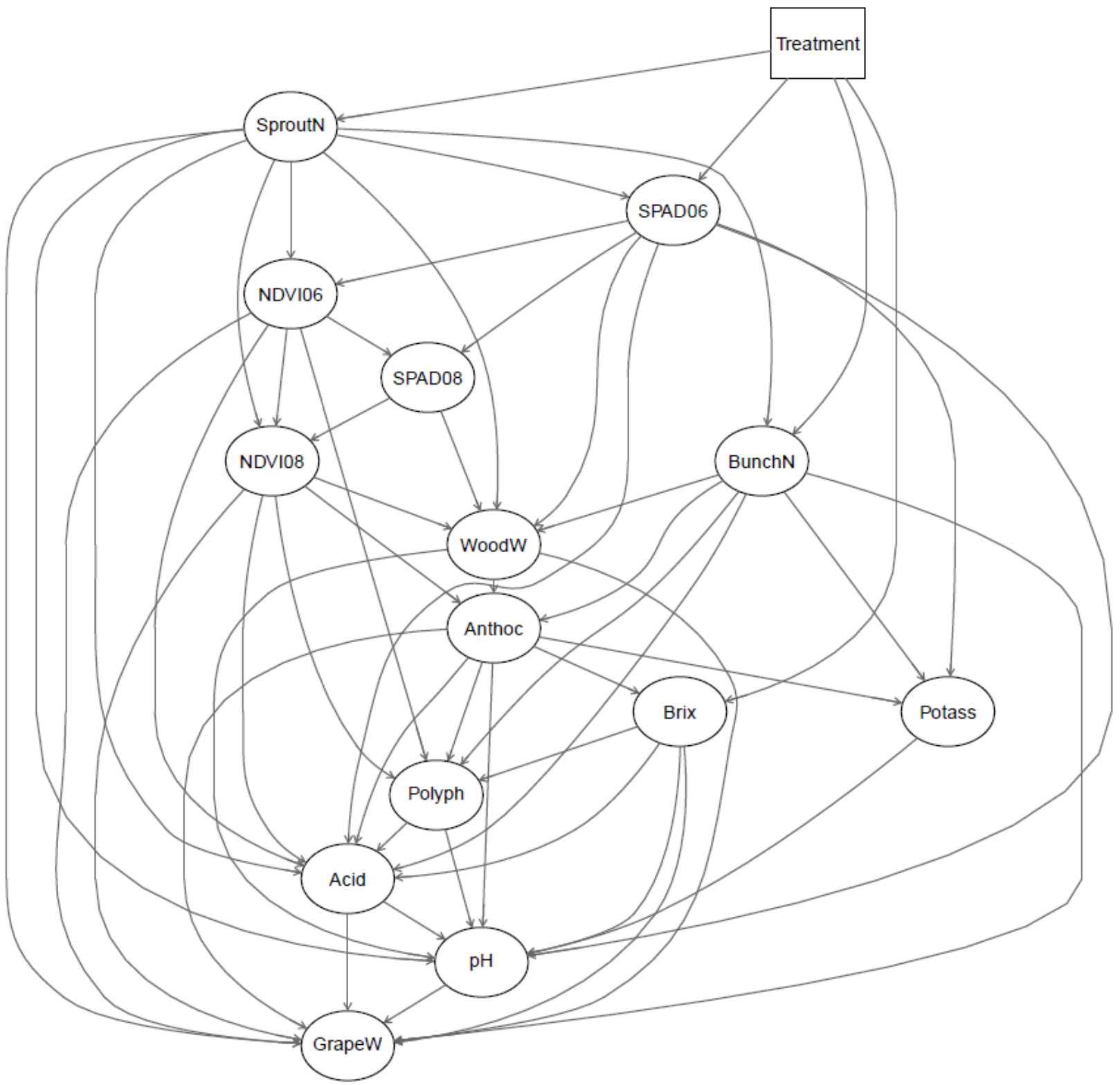
Figure 14: Causal Bayesian network of SANGIOVESE dataset

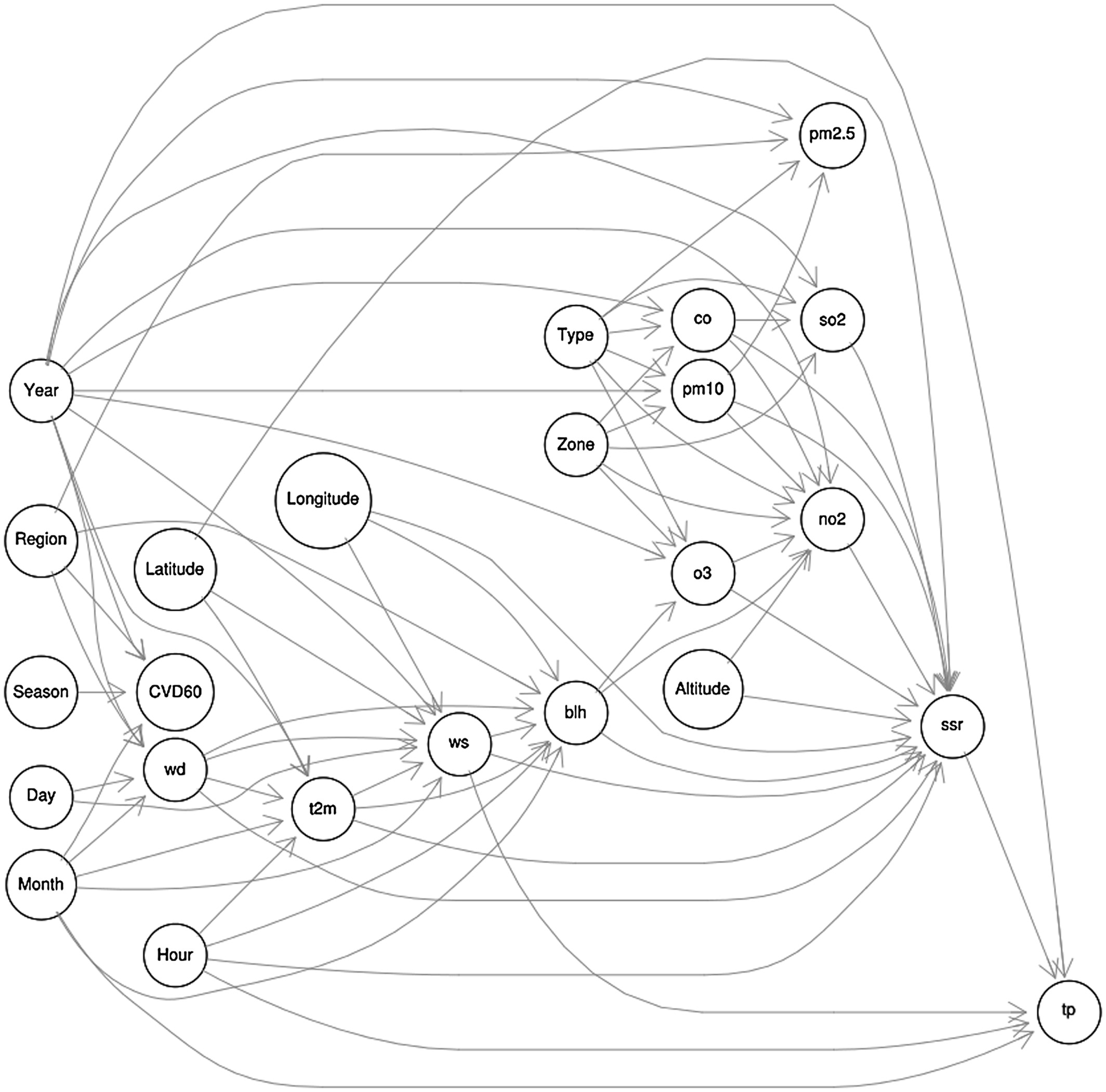
Figure 15: Causal Bayesian network of MEHRA dataset

The causal DAGs of SANGIOVESE, MEHRA, Asia, and Sachs datasets from the BNLearn repository (Scutari & Denis, 2014) are shown in Figs 14, 15, 16, and 17 respectively.

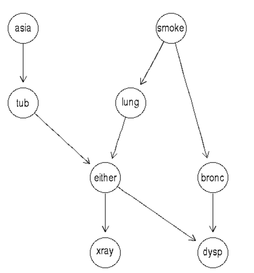
Figure 16: Causal Bayesian network of ASIA/Lung Cancer dataset

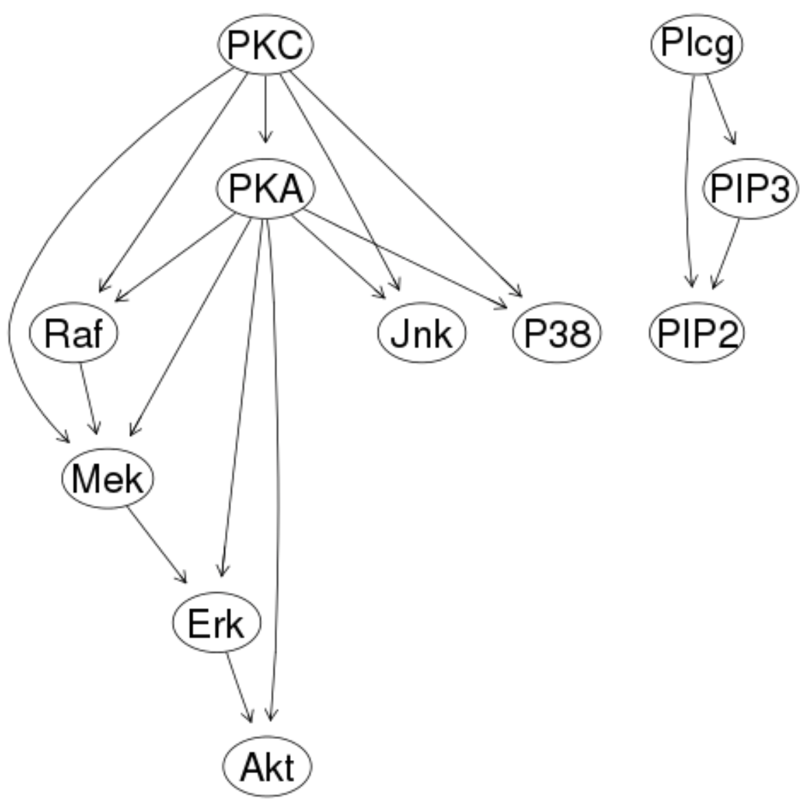
Figure 17: Causal Bayesian network that generates SACHS dataset

Appendix H Architectural/Training Details

We use a multi-layer perceptron with ReLU non-linearity across our experiments, each trained using ADAM optimizer with Dropout and $L_{2}$ weight decay. Table 16 shows the details of neural network architectures and training details of our models for various datasets. $80\%$ of the dataset is used for training and remaining $20\%$ for testing. We observed that gradients on output logits work better than softmax or logsoftmax activated outputs.

S.No.	Dataset	Dataset	Input Size,	Learning Rate	Batch Size	$\lambda_{1}$	Number of	Size of
		Size	Output Size			(ACDE)	Layers	Each Layer
1	COMPAS	6,172	11,2	1e-2	128	50	4	16,16,16,16
2	MEPS	15,830	138,2	1e-3	64	2	3	128,256,256
3	Law School	20,797	15,2	1e-3	64	2	3	64,32,64
4	AutoMPG	398	7,2	1e-2	32	1.5	4	16,16,16,16
5	Boston Housing	506	13,2	1e-2	32	1	4	16,16,16,16
6	Titanic	1,309	10,2	1e-3	64	3	2	64,128
7	Car Evaluation	1,728	6,2	1e-3	64	2	3	64,128,128
8	Heart Disease	303	13,2	1e-2	64	1	3	16,16,16
9	Adult	48842	14,2	1e-2	1024	0.2	3	64,64,64
10	SANGIOVESE	10,000	29,2	1e-2	256	2.3	3	16,16,16
11	SACHS	10,000	10,3	1e-3	64	10	2	16,32
12	ASIA	10,000	7,2	1e-3	64	1	2	32,64
13	MEHRA	10,000	152,2	1e-3	64	2.2	3	32,32,32
14	Synthetic Tabular 1
	$z=\log(1+2x)$	1,000	1,1	1e-2	64	10	2	4,8
	$x\in[0,1]$
15	Synthetic Tabular 2
	$z=\sin{x}+e^{y}$	1,000	2,1	1e-2	64	0.5	2	8,16
	$x,y\in[0,1]$
16	Synthetic Tabular 3
	$z=\sin{x}+e^{y}$	1,000	2,1	1e-3	64	20	2	8,16
	$x,y\in[-2,-1]$
17	Synthetic Tabular 4	10,000	3,2	1e-2	64	1.0	3	12,12,12
	$W:=\mathcal{N}_{w}(0,1)$
	$\vdots$

Table 16: Architectural and training details of all datasets.

References

- mep (2011) Medical expenditure panel survey. https://meps.ahrq.gov/mepsweb/, 2011.
- Agarwal et al. (2018) Agarwal, A., Beygelzimer, A., Dudik, M., Langford, J., and Wallach, H. A reductions approach to fair classification. In Proceedings of the 35th International Conference on Machine Learning, 2018.
- Alvarez-Melis & Jaakkola (2017) Alvarez-Melis, D. and Jaakkola, T. S. A causal framework for explaining the predictions of black-box sequence-to-sequence models. In Proceedings of the 2017 Conference on Empirical Methods in Natural Language Processing, pp. 412–421, 2017.
- Angwin et al. (2016) Angwin, J., Larson, J., Mattu, S., and Kirchner, L. How we analyzed the compas recidivism algorithm, 2016. URL https://www.propublica.org/article/how-we-analyzed-the-compas-recidivism-algorithm.
- Archer & Wang (1993) Archer, N. P. and Wang, S. Application of the back propagation neural network algorithm with monotonicity constraints for two-group classification problems. Decision Sciences, 24(1):60–75, 1993.
- Bahadori et al. (2017) Bahadori, M. T., Chalupka, K., Choi, E., Chen, R., Stewart, W. F., and Sun, J. Causal regularization. arXiv preprint arXiv:1702.02604, 2017.
- Berk (2019) Berk, R. Accuracy and fairness for juvenile justice risk assessments. Journal of Empirical Legal Studies, 16(1):175–194, 2019.
- Berk et al. (2021) Berk, R., Heidari, H., Jabbari, S., Kearns, M., and Roth, A. Fairness in criminal justice risk assessments: The state of the art. Sociological Methods & Research, 50(1):3–44, 2021. doi: 10.1177/0049124118782533.
- Brennan & Oliver (2013) Brennan, T. and Oliver, W. L. Emergence of machine learning techniques in criminology: implications of complexity in our data and in research questions. Criminology & Pub. Pol’y, 12:551, 2013.
- Brue (1993) Brue, S. L. Retrospectives: The law of diminishing returns. Journal of Economic Perspectives, 7(3):185–192, 1993.
- Calabrese & Baldwin (2001) Calabrese, E. J. and Baldwin, L. A. U-shaped dose-responses in biology, toxicology, and public health. Annual review of public health, 22(1):15–33, 2001.
- Chattopadhyay et al. (2019) Chattopadhyay, A., Manupriya, P., Sarkar, A., and Balasubramanian, V. N. Neural network attributions: A causal perspective. In Chaudhuri, K. and Salakhutdinov, R. (eds.), Proceedings of the 36th International Conference on Machine Learning, volume 97 of Proceedings of Machine Learning Research, pp. 981–990, Long Beach, California, USA, 09–15 Jun 2019. PMLR.
- Daniels & Velikova (2010) Daniels, H. and Velikova, M. Monotone and partially monotone neural networks. IEEE Transactions on Neural Networks, 21(6):906–917, 2010.
- Dash et al. (2022) Dash, S., Balasubramanian, V. N., and Sharma, A. Evaluating and mitigating bias in image classifiers: A causal perspective using counterfactuals. In Proceedings of the IEEE/CVF Winter Conference on Applications of Computer Vision, pp. 915–924, 2022.
- Dua & Graff (2017) Dua, D. and Graff, C. UCI machine learning repository, 2017. URL http://archive.ics.uci.edu/ml.
- Dugas et al. (2009) Dugas, C., Bengio, Y., Bélisle, F., Nadeau, C., and Garcia, R. Incorporating functional knowledge in neural networks. Journal of Machine Learning Research, 10(6), 2009.
- Ferguson (2014) Ferguson, A. G. Big data and predictive reasonable suspicion. U. Pa. L. Rev., 163:327, 2014.
- Flanders & Augestad (2008) Flanders, W. D. and Augestad, L. B. Adjusting for reverse causality in the relationship between obesity and mortality. International Journal of Obesity (2005), 32 Suppl 3:S42–46, August 2008. ISSN 1476-5497. doi: 10.1038/ijo.2008.84.
- Fraser et al. (2016) Fraser, A., Lawlor, D. A., and Howe, L. D. Nonlinear Exposure-Outcome Associations and Public Health Policy. JAMA, 315(12):1286–1287, March 2016. ISSN 0098-7484. doi: 10.1001/jama.2015.18023.
- Goodman et al. (2018) Goodman, S. N., Goel, S., and Cullen, M. R. Machine learning, health disparities, and causal reasoning. Annals of internal medicine, 169(12):883–884, 2018.
- Goyal et al. (2019a) Goyal, Y., Feder, A., Shalit, U., and Kim, B. Explaining classifiers with causal concept effect (cace). arXiv preprint arXiv:1907.07165, 2019a.
- Goyal et al. (2019b) Goyal, Y., Wu, Z., Ernst, J., Batra, D., Parikh, D., and Lee, S. Counterfactual visual explanations. In Proceedings of the 36th International Conference on Machine Learning, volume 97 of Proceedings of Machine Learning Research, pp. 2376–2384, 09–15 Jun 2019b.
- Gupta et al. (2019) Gupta, A., Shukla, N., Marla, L., Kolbeinsson, A., and Yellepeddi, K. How to incorporate monotonicity in deep networks while preserving flexibility? arXiv preprint arXiv:1909.10662, 2019.
- Gupta et al. (2021) Gupta, A., Marla, L., Sun, R., Shukla, N., and Kolbeinsson, A. Pender: Incorporating shape constraints via penalized derivatives. Proceedings of the AAAI Conference on Artificial Intelligence, 35(13):11536–11544, May 2021.
- Gupta et al. (2016) Gupta, M., Cotter, A., Pfeifer, J., Voevodski, K., Canini, K., Mangylov, A., Moczydlowski, W., and Van Esbroeck, A. Monotonic calibrated interpolated look-up tables. J. Mach. Learn. Res., 17(1):3790–3836, January 2016. ISSN 1532-4435.
- Hornik et al. (1989) Hornik, K., Stinchcombe, M., and White, H. Multilayer feedforward networks are universal approximators. Neural networks, 2(5):359–366, 1989.
- Janzing (2019) Janzing, D. Causal regularization. In Advances in Neural Information Processing Systems, pp. 12704–12714, 2019.
- Kahneman & Tversky (2013) Kahneman, D. and Tversky, A. Choices, values, and frames. In Handbook of the fundamentals of financial decision making: Part I, pp. 269–278. World Scientific, 2013.
- Khademi & Honavar (2020) Khademi, A. and Honavar, V. A causal lens for peeking into black box predictive models: Predictive model interpretation via causal attribution. arXiv 2008.00357, 2020.
- Kilbertus et al. (2017) Kilbertus, N., Rojas Carulla, M., Parascandolo, G., Hardt, M., Janzing, D., and Schölkopf, B. Avoiding discrimination through causal reasoning. In Advances in Neural Information Processing Systems, 2017.
- Kocaoglu et al. (2018) Kocaoglu, M., Snyder, C., Dimakis, A. G., and Vishwanath, S. CausalGAN: Learning causal implicit generative models with adversarial training. In International Conference on Learning Representations, 2018.
- Kyono et al. (2020) Kyono, T., Zhang, Y., and van der Schaar, M. Castle: Regularization via auxiliary causal graph discovery. In Advances in Neural Information Processing Systems, volume 33, pp. 1501–1512, 2020.
- Luk et al. (2001) Luk, J., Gross, P., and Thompson, W. W. Observations on mortality during the 1918 influenza pandemic. Clinical Infectious Diseases, 33(8):1375–1378, 2001.
- Pearl (2001) Pearl, J. Direct and indirect effects. In Proceedings of the Seventeenth conference on Uncertainty in artificial intelligence, 2001.
- Pearl (2009) Pearl, J. Causality. Cambridge university press, 2009.
- Pitis et al. (2020) Pitis, S., Creager, E., and Garg, A. Counterfactual data augmentation using locally factored dynamics. In Advances in Neural Information Processing Systems, volume 33, pp. 3976–3990. Curran Associates, Inc., 2020.
- Ribeiro et al. (2016) Ribeiro, M. T., Singh, S., and Guestrin, C. Why should i trust you?: Explaining the predictions of any classifier. In Proceedings of the 22nd ACM SIGKDD International Conference on Knowledge Discovery and Data Mining, pp. 1135–1144. ACM, 2016.
- Rieger et al. (2020) Rieger, L., Singh, C., Murdoch, W., and Yu, B. Interpretations are useful: Penalizing explanations to align neural networks with prior knowledge. In III, H. D. and Singh, A. (eds.), Proceedings of the 37th International Conference on Machine Learning, volume 119 of Proceedings of Machine Learning Research, pp. 8116–8126, Virtual, 13–18 Jul 2020. PMLR.
- Ross et al. (2017) Ross, A. S., Hughes, M. C., and Doshi-Velez, F. Right for the right reasons: Training differentiable models by constraining their explanations. In Proceedings of the Twenty-Sixth International Joint Conference on Artificial Intelligence, IJCAI-17, pp. 2662–2670, 2017. doi: 10.24963/ijcai.2017/371.
- Salkind (2010) Salkind, N. J. Encyclopedia of research design (Vols. 1-0): U-shaped curve. SAGE Publications, Inc., 2010.
- Schwab et al. (2020) Schwab, P., Linhardt, L., Bauer, S., Buhmann, J. M., and Karlen, W. Learning counterfactual representations for estimating individual dose-response curves. In Proceedings of the AAAI Conference on Artificial Intelligence, volume 34, pp. 5612–5619, 2020.
- Scutari & Denis (2014) Scutari, M. and Denis, J. Bayesian Networks: With Examples in R. Chapman & Hall/CRC Texts in Statistical Science. Taylor & Francis, 2014. ISBN 9781482225587.
- Sen et al. (2018) Sen, S., Mardziel, P., Datta, A., and Fredrikson, M. Supervising feature influence. arXiv preprint arXiv:1803.10815, 2018.
- Shen et al. (2021) Shen, Z., Liu, J., He, Y., Zhang, X., Xu, R., Yu, H., and Cui, P. Towards out-of-distribution generalization: A survey. CoRR, abs/2108.13624, 2021.
- Shimizu et al. (2006) Shimizu, S., Hoyer, P. O., Hyvärinen, A., Kerminen, A., and Jordan, M. A linear non-gaussian acyclic model for causal discovery. Journal of Machine Learning Research, 7(10), 2006.
- Sill (1998) Sill, J. Monotonic networks. In Advances in neural information processing systems, pp. 661–667, 1998.
- Sivaraman et al. (2020) Sivaraman, A., Farnadi, G., Millstein, T., and Broeck, G. V. d. Counterexample-guided learning of monotonic neural networks. arXiv preprint arXiv:2006.08852, 2020.
- Srinivas & Fleuret (2018) Srinivas, S. and Fleuret, F. Knowledge transfer with Jacobian matching. In Proceedings of the 35th International Conference on Machine Learning, volume 80 of Proceedings of Machine Learning Research, pp. 4723–4731. PMLR, 10–15 Jul 2018.
- Suter et al. (2019) Suter, R., Miladinovic, D., Schölkopf, B., and Bauer, S. Robustly disentangled causal mechanisms: Validating deep representations for interventional robustness. In International Conference on Machine Learning, pp. 6056–6065. PMLR, 2019.
- VanderWeele (2011) VanderWeele, T. J. Controlled direct and mediated effects: definition, identification and bounds. Scandinavian Journal of Statistics, 38(3):551–563, 2011.
- Wang et al. (2021) Wang, Y., Liu, F., Chen, Z., Lian, Q., Hu, S., Hao, J., and Wu, Y.-C. Contrastive ace: Domain generalization through alignment of causal mechanisms. arXiv 2106.00925, 2021.
- Wightman et al. (1998) Wightman, L., Ramsey, H., and Council, L. S. A. LSAC National Longitudinal Bar Passage Study. LSAC research report series. Law School Admission Council, 1998.
- Yadu et al. (2021) Yadu, A., Suhas, P. K., and Sinha, N. Class specific interpretability in cnn using causal analysis. In 2021 IEEE International Conference on Image Processing (ICIP), pp. 3702–3706, 2021. doi: 10.1109/ICIP42928.2021.9506118.
- Yang et al. (2020) Yang, M., Liu, F., Chen, Z., Shen, X., Hao, J., and Wang, J. Causalvae: Structured causal disentanglement in variational autoencoder. arXiv preprint arXiv:2004.08697, 2020.
- Yang & Natarajan (2013) Yang, S. and Natarajan, S. Knowledge intensive learning: Combining qualitative constraints with causal independence for parameter learning in probabilistic models. In Blockeel, H., Kersting, K., Nijssen, S., and Železný, F. (eds.), Machine Learning and Knowledge Discovery in Databases, pp. 580–595, Berlin, Heidelberg, 2013. Springer Berlin Heidelberg. ISBN 978-3-642-40991-2.
- You et al. (2017) You, S., Ding, D., Canini, K., Pfeifer, J., and Gupta, M. Deep lattice networks and partial monotonic functions. In Guyon, I., Luxburg, U. V., Bengio, S., Wallach, H., Fergus, R., Vishwanathan, S., and Garnett, R. (eds.), Advances in Neural Information Processing Systems, volume 30, pp. 2981–2989. Curran Associates, Inc., 2017.
- Zhang & Bareinboim (2018) Zhang, J. and Bareinboim, E. Fairness in decision-making—the causal explanation formula. In Proceedings of the AAAI Conference on Artificial Intelligence, volume 32, 2018.
- Zhu et al. (2020) Zhu, S., Ng, I., and Chen, Z. Causal discovery with reinforcement learning. In International Conference on Learning Representations, 2020.
- Zmigrod et al. (2019) Zmigrod, R., Mielke, S. J., Wallach, H., and Cotterell, R. Counterfactual data augmentation for mitigating gender stereotypes in languages with rich morphology. arXiv preprint arXiv:1906.04571, 2019.