Probing quantum chaos in multipartite systems

Abstract

Understanding the emergence of quantum chaos in multipartite systems is challenging in the presence of interactions. We show that the contribution of the subsystems to the global behavior can be revealed by probing the full counting statistics of the local, total, and interaction energies. As in the spectral form factor, signatures of quantum chaos in the time domain dictate a dip-ramp-plateau structure in the characteristic function, i.e., the Fourier transform of the eigenvalue distribution. With this approach, we explore the fate of chaos in interacting subsystems that are locally maximally chaotic. Global quantum chaos can be suppressed at strong coupling, as illustrated with coupled copies of random-matrix Hamiltonians and of the Sachdev-Ye-Kitaev model. Our method is amenable to experimental implementation using single-qubit interferometry.

I Introduction

Identifying signatures of chaos in the quantum domain remains a nontrivial task in complex systems [1]. Quantum chaos has manifold applications and appears in different fields involving the study of many-body complex quantum systems [2, 3, 4], statistical mechanics of isolated quantum systems [5, 6], anti-de Sitter black holes [7, 8, 9, 10, 11], holographic quantum matter [12], and quantum information science [13, 14], among other examples. Several diagnostic tools for quantum chaos have been proposed. They include the spectral form factor (SFF) [1], fidelity decay in short-time [15] and long-time regimes [16], Loschmidt echo (LE) [17], out-of-time-order correlator (OTOC) [18], quantum circuit complexity [19, 20], etc. Connections among these diagnostics have been explored in specific areas ranging from many-body systems to quantum field theory [17, 21, 22, 23, 24, 25]. More recently, diagnostics of quantum chaos have been extended to open systems to account for the effect of decoherence and dissipation [26, 27, 28, 29, 30, 31, 32, 33, 34, 35, 36, 37].

A prominent signature of quantum chaos is the repulsion among energy levels. For instance, the spacing between nearest-neighbor levels follows the Wigner-Dyson distribution in quantum chaotic systems, while it is described by Poisson statistics in the presence of conserved quantities (e.g., in integrable systems) [38]. The SFF is proportional to $|Z(\beta+it)/Z(\beta)|^{2}$, where $Z(\cdot$) is the partition function and $\beta=1/k_{B}T$. This quantity probes the level statistics of both close and far-separated energy eigenvalues, providing a tool to detect the ergodic nature of the system [1]. For a generic chaotic system, the SFF exhibits a dip-ramp-plateau structure [see e.g., Fig. 1]. Its short-time decay forms a slope. The physical origin of the subsequent ramp is the long-range repulsion between energy levels [11]. The transition from the slope to the ramp forms the dip. The final plateau originates from the finite Hilbert space dimension and approaches a constant value $Z(2\beta)$/$Z(\beta)^{2}$ in the absence of degeneracies in the energy spectrum. The SFF has been widely employed in the study of the discrete energy spectrum of quantum chaotic systems [39, 40, 41, 42, 11, 43, 44, 45].

Quantum chaotic systems composed of multipartite subsystems subject to generic interactions typically have a complicated energy spectrum [46, 47, 48, 45]. We shall focus on a global subsystem composed of strongly-chaotic subsystems, interacting with each other. In this setting, any subsystem can be seen as an open quantum system embedded in an environment, composed of the remaining subsystems. The subsystem dynamics is thus governed by dissipative quantum chaos [1], which is currently under exhaustive study [29, 49, 50, 30, 33, 51, 34, 37, 52, 53]. We shall depart from the standard practice of assuming an effective open quantum dynamics, as ubiquitously done in the literature. Instead, we will account for the exact unitary dynamics of the global composite system, with no approximations (e.g., without invoking the Markovian description or an effective master equation). The above diagnostics can be employed to detect global quantum chaos in multipartite systems [48]. However, apart from proposals like the fidelity-based SFF [34, 37] and the related partial SFF [45], they are not suited to directly detect how chaotic behavior stems from the subsystems and their interactions. In this work, we provide an experimentally realizable approach to this end by considering the measurement of an energy observable $X$, which can be the Hamiltonian of a subsystem or the interaction energy. As measurement outcomes are stochastic, we propose to study the full counting statistics, characterized by the eigenvalue distribution of $X$ at thermal equilibrium. Its Fourier transform, the characteristic function, reveals chaotic behavior through the dip-ramp-plateau structure. Its analysis shows that strong interactions among the different subsystems can suppress the global chaotic behavior of the multipartite system, even when the subsystems are maximally chaotic, as revealed by the study of global and local observables. This scheme not only provides a convenient theoretical tool to diagnose quantum chaos in complex multipartite quantum systems, but it can be experimentally realized by using single-qubit interferometry with an ancillary qubit.

Our paper is organized as follows. In Sec. II, we introduce the characteristic function of an energy observable, which is then used as a tool to detect the chaotic features stemming from the subsystems and their interactions in Sec. III. Then, we employ this method to analyze the chaotic behavior in multipartite systems sampled from the Gaussian orthogonal ensemble ($\mathrm{GOE}$) in Random Matrix Theory (RMT) [2, 54] in Sec. IV and the coupled Sachdev–Ye–Kitaev (cSYK) models [55, 56, 57, 58, 59, 60, 61, 62, 63, 64] in Sec. V. Finally, we summarize in Sec. VI with concluding remarks and a brief discussion of potential applications.

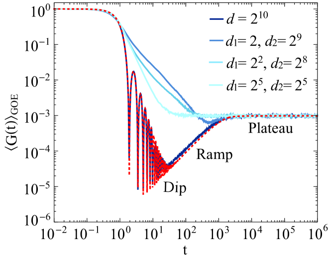
Figure 1: The dip-ramp-plateau structure: an indicator of quantum chaoticity. The absolute square value of the generating function $G(t)$ for the total energy distribution averaged over $\mathrm{GOE}(d)$ ($d=2^{10}$) and $\mathrm{GOE}(d_{1})\otimes\mathrm{GOE}(d_{2})$ ($d_{1}d_{2}=d$), with 500 independent realizations, and $\beta=0.01$. Analytical Eq. (7) for $\mathrm{GOE}(d)$ is depicted in red color. For systems with less chaoticity than the full GOE, the span of the ramp will shrink or even vanish.

II The characteristic function of the energy observable $X$

Let $\mathcal{H}=\bigotimes_{l}\mathcal{H}_{l}$ be the Hilbert space of a multipartite system and $X$ be an energy observable of a local subsystem in the subspace $\bigotimes_{k}\mathcal{H}_{k}$ $\subseteq\mathcal{H}$. We focus on the Hamiltonian of the subsystems (local energy) and the interaction energy, as choices of the observable $X$. The probability distribution of the observable $X$ with eigenvalues $\{x\}$ averaged over an initial thermal equilibrium state $\rho_{\mathrm{th}}=e^{-\beta H}/Z(\beta)$ is [65]

$$P(x)=\mathrm{tr}\left[\rho_{\mathrm{th}}\delta(X-x)\right].$$ (1)

The eigenvalue probability distribution $P(x)$ encodes the full counting statistics of the observable $X$, that is, the probability to find the system in an eigenstate with eigenvalue $x$ when prepared in the state $\rho_{\mathrm{th}}$. In terms of the integral representation of the Dirac delta function, the probability distribution can be expressed as the Fourier transform

$$P(x)=\frac{1}{2\pi}\int_{-\infty}^{+\infty}g(t)e^{-itx}dt,$$ (2)

of the characteristic (moment generating) function

$$g(t)=\mathrm{tr}\left(\rho_{\mathrm{th}}e^{itX}\right),$$ (3)

that captures the statistical properties of the spectrum of the observable $X$. While in the following we refer to $t$ as a time variable, it is to be understood as the Fourier conjugate to $x$.

Experimentally, the characteristic function Eq. (3) can be measured by introducing an auxiliary qubit coupled to the system. This technique known as single-qubit interferometry has been widely used in measuring fidelity decay [27], form factors of Floquet operators [66], local density of states [67], LE [68, 69], work statistics [70, 71, 72], Lee-Yang zeros [73, 74, 75], OTOC [76], quantum-state reconstruction of dark systems [77], full distribution of many-body observables [65], and SFF [78]. The key procedure is to perform a controlled $X$ gate conditioning on the auxiliary qubit, i.e.,

$$U(t)=\left|1\right\rangle\left\langle 1\right|\otimes\exp(itX)+\left|0\right\rangle\left\langle 0\right|\otimes\openone.$$ (4)

This allows us to recover the real and imaginary parts of Eq. (3) by measuring a pair of Pauli operators on the ancillary qubit [65], i.e., Re$(g(t))=$tr$(\sigma_{z}\rho_{\mathrm{ancillary}})$ and Im$(g(t))=$tr$(\sigma_{y}\rho_{\mathrm{ancillary}})$, where $\rho_{\mathrm{ancillary}}=\mathrm{tr}_{\mathrm{system}}(\mathrm{H}\otimes\openone U(t)\left|+\right\rangle\left\langle+\right|\otimes\rho_{\mathrm{th}}U^{{\dagger}}(t)\mathrm{H}\otimes\openone)$, $\mathrm{H}$ is the Hadamard gate, and $\left|+\right\rangle=(\left|0\right\rangle+\left|1\right\rangle)/\sqrt{2}$.

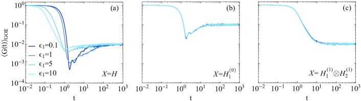
Figure 2: Chaos is suppressed by enhancing the interaction in a bipartite system. (a) Equation (5) averaged over GOEs for observables $X=H$ ($H=H_{1}^{(0)}+H_{2}^{(0)}+\epsilon_{1}H_{1}^{(1)}\otimes H_{2}^{(1)}$) with coupling strength $\epsilon_{1}=0.1,$ $1,$ $5,$ and $10$ respectively. $H_{1}^{(0,1)}$ and $H_{2}^{(0,1)}$ are sampled from GOE independently, with 500 realizations, $d_{1}=d_{2}=10$, and $\beta=0.01$ (for other temperature and number of realizations, see in Appendix B). The size of dip-ramp shrinks when the coupling constant $\epsilon_{1}$ is enhancing, implying that chaos is suppressed. The GOE averaged $G(t)$ is depicted with $X=H_{1}^{(0)}$ in (b) and $X=H_{1}^{(1)}\otimes H_{2}^{(1)}$ in (c), respectively, in which $H_{1}^{(1)}\otimes H_{2}^{(1)}$ with no obvious dip-ramp-plateau structure plays an important role in attenuating the chaoticity.

III A probe for quantum chaos in multipartite systems

In what follows, we consider the absolute square value of the generating function in Eq. (3), i.e.,

$$G(t)=|g(t)|^{2}=|\mathrm{tr}\left(\rho_{\mathrm{th}}e^{itX}\right)|^{2},\text{ }t\in[0,\infty),$$ (5)

as a tool for probing quantum chaos in multipartite systems, identifying contributions from the subsystems and their interactions. The choice $X=H_{j}$ represents the local energy that can be employed to diagnose the chaotic behavior contributed by the $j$th subsystem in an $N$-partite system. By contrast, the observable $X=H_{j}\otimes H_{k}\otimes H_{l}$ can be used to detect signature of quantum chaos attributed to the interactions among subsystems $j$, $k$, and $l$.

The original motivation behind Eq. (5) is based on the fact that when the observable $X$ is chosen as the global Hamiltonian $X=H$ $\left(H\in\mathcal{H}\right)$, the absolute square value of the generating function in Eq. (5) turns out to be $G(t)=\left|\frac{Z(\beta+it)}{Z(\beta)}\right|^{2}$, which equals the SFF [79, 11, 23] and can be interpreted as the fidelity between the initial coherent Gibbs state (or a thermofield double state) and the state resulting from its evolution [44, 34]. In addition, when $X$ is a small perturbation of the Hamiltonian $H$, i.e., $H=H_{0}+X$, and commutes with $H$ (or $H_{0}$), Eq. (5) is similar to the LE $G(t)=\left|\left\langle\psi_{0}\right|e^{itH}e^{-itH_{0}}\left|\psi_{0}\right\rangle\right|^{2}$, which captures the overlap between two identical initial states $(\left|\psi_{0}\right\rangle)$ evolving under slightly different Hamiltonians $H$ and $H_{0}$ [17]. Note that according to the  Baker–Campbell–Hausdorff formula, Eq. (5) and the LE differ in the general case, when $[X,H]\neq 0$.

We emphasize that the observable $X$ in Eq. (5) is not required to represent a small perturbation or to commute with $H$. When it describes the local energy of a subsystem $\bigotimes_{k}\mathcal{H}_{k}$ $\subseteq\mathcal{H}$, Eq. (5) provides the possibility to directly detect the chaotic behavior contributed by the subsystems or interactions to the global multipartite system. It can be used to either diagnose quantum chaos of a one-partite system (as done by the SFF) or a structured multipartite system. To support this observation, we illustrate its use in the following examples involving coupled random-matrix Hamiltonians and the coupled SYK model.

IV Probing the chaoticity in coupled random-matrix Hamiltonians

Consider a $N-$partite system with a general Hamiltonian of the form

$$H=\sum_{j=1}^{N}H_{j}^{(0)}+\epsilon_{1}\sum_{j<k=2}^{N}H_{j}^{(1)}\otimes H_{k}^{(1)}+\cdots+\epsilon_{N-1}\bigotimes_{j=1}^{N}H_{j}^{(N-1)},$$ (6)

where $H_{j}^{(0)}$ is the Hamiltonian of the $j$th subsystem and $\epsilon_{l-1}$ is the coupling constant for the $l$-partite interaction $\bigotimes_{j=1}^{l}H_{j}^{(l-1)}$.

For the sake of illustration, let us sample the Hamiltonians from the Gaussian orthogonal ensemble ($\mathrm{GOE}$) [2, 54], which is a paradigmatic random matrix ensemble for physical applications involving systems with time-reversal symmetry and exhibiting quantum chaos. GOE is the ensemble of real symmetric matrices, whose elements are chosen at random from a Gaussian distribution. The joint probability density of $H_{j}\in\mathrm{GOE(}d_{j}\mathrm{)}$ ($d_{j}$ denotes the dimension of the Hilbert space $\mathcal{H}_{j}$) is proportional to $\exp(-\frac{1}{2\sigma^{2}}\mathrm{tr}H_{j}^{2})$, where $\sigma$ is the standard deviation of the random matrix elements of $H_{j}$.

The first example we consider is $N=1$ and $X=H$. In this scenario, we focus on $H\in\mathrm{GOE(}d\mathrm{)}$ and $H\in\mathrm{GOE(}d_{1}\mathrm{)}\otimes\mathrm{GOE(}d_{2}\mathrm{)}$ ($d_{1}d_{2}=d$) as an example. Equation (5) averaged over the full GOEs [i.e., GOE(d)] yields

$$\left\langle G(t)\right\rangle_{\mathrm{GOE}}\doteq\frac{\left\langle Z(2\beta)\right\rangle_{\mathrm{GOE}}\cdot C_{\mathrm{GOE}}+\left|\left\langle Z(\beta+it)\right\rangle_{\mathrm{GOE}}\right|^{2}}{\left\langle Z(\beta)\right\rangle_{\mathrm{GOE}}^{2}},$$ (7)

where $\left\langle\cdot\right\rangle$ represents the ensemble average and $\doteq$ denotes the annealing approximation [11]. In Eq. (7), the GOE averaged partition function is given by (see Appendix A)

$$\left\langle Z(x)\right\rangle_{\mathrm{GOE}}=\frac{\sqrt{d}\mathrm{I}_{1}(2\sigma\sqrt{d}x)}{\sigma x},$$ (8)

where $\mathrm{I}_{n}(\cdot)$ is the modified Bessel function of first kind and order $n$, and the coefficient reads

$$C_{\mathrm{GOE}}=\left\{\begin{array}[]{ll}\frac{t\sigma}{\sqrt{d}}-\frac{t\sigma}{2\sqrt{d}}\ln\left(1+\frac{t\sigma}{\sqrt{d}}\right),&t\leq 2\sqrt{d}/\sigma,\\ 2-\frac{t\sigma}{2\sqrt{d}}\ln\frac{t+\sqrt{d}/\sigma}{t-\sqrt{d}/\sigma}.&t>2\sqrt{d}/\sigma.\end{array}\right.$$ (9)

As shown by the red dotted curve (or the dark blue curve by numerical simulations) in Fig. 1, Eq. (7) exhibits a typical feature of quantum chaos, namely a dip-ramp-plateau structure. The early decay from unit value comes to an end, forming a dip (also known as correlation hole) with the onset of a ramp. The latter extends until it saturates at a plateau value at the characteristic plateau time $t_{\mathrm{plateau}}=2\sqrt{d}/\sigma$ [see Eq. (9)]. The existence of the ramp, a period of linear growth of $\left\langle G(t)\right\rangle_{\mathrm{GOE}}$, is a consequence of the repulsion between long-range energy levels [11]. This long-range repulsion causes the energy levels to be anticorrelated. The plateau stems from the discrete energy spectrum, whose height is $\left\langle Z(2\beta)\right\rangle_{\mathrm{GOE}}/\left\langle Z(\beta)\right\rangle_{\mathrm{GOE}}^{2}$. Similar chaotic features have been studied in the Gaussian Unitary Ensemble (GUE) [44, 80, 34], Gaussian ensembles under infinite temperature [81], and Sachdev–Ye–Kitaev (SYK) models [11, 82, 83].

For systems with less chaoticity than the full GOE, the span of the ramp will shrink or even disappear (see light blue curves in Fig. 1).

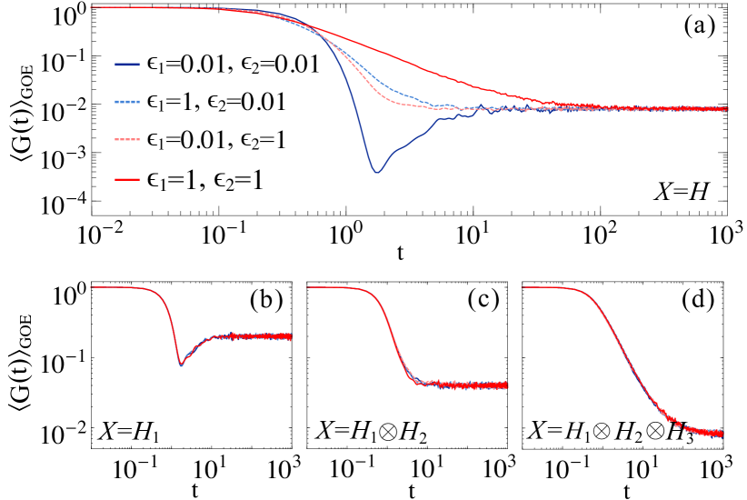
Figure 3: Chaos is suppressed by enhancing the interactions among a tripartite system. Equation (5) averaged with GOEs for observables (a) $X=H$, (b) $X=H_{1}$, (c) $X=H_{1}\otimes H_{2}$, and (d) $X=H_{1}\otimes H_{2}\otimes H_{3}$, respectively. $H_{1}$, $H_{2}$, and $H_{3}$ are sampled from GOE independently, with 500 realizations, $d_{1}=d_{2}=d_{3}=5$, and $\beta=0.01$.

Without loss of generality, we then consider a bipartite system with $H_{1,2}^{(0,1)}$ independently sampled from GOEs. As the total system is composed of two partitions each described by a random-matrix Hamiltonian, it is not surprising that in the absence of (or weak) interactions the full system exhibits visible dip-ramp-plateau structure when choosing $X=H$ [see the dark blue curve in Fig. 2 (a)]. However, when the coupling strength $\epsilon_{1}$ between subsystems $1$ and $2$ is enhanced, the dip-ramp-plateau structure gradually washes out [light blue curves in Fig. 2 (a)].

To account for this phenomenon, we look at the characteristic function for different choices of the observable $X=H_{1}^{(0)}$ in Fig. 2 (b) and $X=H_{1}^{(1)}\otimes H_{2}^{(1)}$ in Fig. 2 (c) and show how these choices identify the contributions to quantum chaos by the first subsystem and the interactions between subsystems $1$ and $2$. Obviously, $H_{1}^{(1)}\otimes H_{2}^{(1)}$ plays an important role in diminishing the chaotic behavior, since the characteristic function reflects no obvious ramp structure. Indeed, from the perspective of the nearest-neighbor level distribution, the Kronecker product of random matrices will tend to break the Wigner-Dyson distribution under certain conditions [84]. When the coupling is enhanced, the interaction term $H_{1}^{(1)}\otimes H_{2}^{(1)}$ dominates, and the chaoticity of the whole system is gradually suppressed.

Similar phenomena exist in more structured systems, as shown in Fig. 3 for a tripartite system. For simplicity, we only consider $H_{1,2,3}^{(0)}=$ $H_{1,2,3}^{(1)}=H_{1,2,3}^{(2)}$ and omit the superscript therein. Both bipartite interactions (e.g., $H_{1}\otimes H_{2}$), and the tripartite interaction $H_{1}\otimes H_{2}\otimes H_{3}$ play an import role in decreasing the chaoticity of the composite global system, while the local chaotic nature of each subsystem can be detected by choosing a local observable (e.g. $X=H_{1}$) even at strong coupling.

It is worthwhile to note that the presence of interactions could also induce chaos if the interaction tend to mix the subsystems, just as shown in the coupled kicked rotors [46].

V Coupled Sachdev-Ye-Kitaev model

The second example we consider is the coupled Sachdev-Ye-Kitaev (cSYK) model [56, 57, 58, 55, 59, 60, 61, 62, 63, 64]. A system composed of $2N$ Majorana fermions is divided into two separated sides and each subsystem is described by the SYK model [85, 86]. We consider the left and right SYK Hamiltonians $H_{L,R}$ with a bilinear coupling $H_{b}$. The total Hamiltonian of the cSYK model reads

$$H=H_{L}+H_{R}+\mu H_{b}=\sum_{\alpha=L,R}\sum_{1\leq k<l<m<n\leq N}J_{klmn}\chi_{k}^{\alpha}\chi_{l}^{\alpha}\chi_{m}^{\alpha}\chi_{n}^{\alpha}+\mu i\sum_{k=1}^{N}K_{kk}\chi_{k}^{L}\chi_{k}^{R},$$ (10)

where $\mu$ controls the strength of the the bilinear coupling and $\chi_{k}$ denote Majorana fermion operators satisfying the anticommutation relations $\{\chi_{k},\chi_{l}\}=\delta_{kl}$. $J_{klmn}$ and $K_{kk}$ are random coupling constants independently sampled from Gaussian distributions with zero expectation values and $\left\langle J_{klmn}^{2}\right\rangle=\frac{3!J^{2}}{N^{3}}$, $\left\langle K_{kk}^{2}\right\rangle=\frac{K^{2}}{N^{2}}$. A similar model has been used to study the holographic duality of an eternal traversable wormhole: By preparing the SYK model in a thermofield double state and turning on the coupling between the two sides, the wormhole is traversable in the context of gravity [55].

Figure 4 shows the numerical result for the disorder-averaged $\langle G(t)\rangle$, in agreement with the random matrix theory. From Fig. 4(b), we see that the bilinear coupling plays an important role in controlling the chaotic behavior of the whole system, as the generating function has no obvious dip-ramp-plateau structure. The chaotic character of the system is robust when the bilinear coupling is weak ($\mu\lesssim 0.1$). When enhancing the coupling, the dip-ramp-plateau structure of the entire system is gradually washed out [Fig. 4(a)]. This implies that the entire system becomes less chaotic when the bilinear coupling is strong, even when the chaoticity of the subsystems remain consistent. As in the GOE example, the chaotic nature of each subsystem can be detected by choosing a local observable (e.g. $X=H_{L}$), as shown in Fig. 4(b).

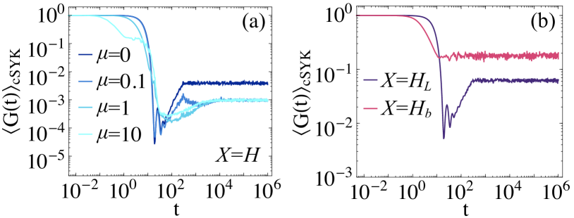
Figure 4: Chaotic behavior in a coupled Sachdev-Ye-Kitaev (cSYK) model. Equation (5) averaged with cSYK for observables (a) $X=H$, (b) $X=H_{L}$, and $X=H_{b}$, respectively. The Hamiltonian is sampled by $500$ realizations with $2N=20$, $\beta=0$, and $J=K=1$.

VI Discussion and conclusion

We have introduced a protocol to directly detect quantum chaos in interacting multipartite systems by measuring the statistical distribution of an energy observable $X$ at thermal equilibrium. Specifically, we make use of the absolute square value $G(t)$ of the generating function of the eigenvalue distribution associated with the observable $X$. When the observable equals the total Hamiltonian, $G(t)$ reduces to the SFF. For local observables, chaotic features give rise to a dip-ramp-plateau structure in $G(t)$, which is similar to that in SFF. $G(t)$ directly detects the contributions to quantum chaos in a composite system from different subsystems by choosing the observable for $k$-partite interactions. We have shown that the coupling of chaotic systems can give rise to the suppression of quantum chaos in the composite system, as the interaction strength among the subsystems is increased. From the perspective of decoherence, sampling the eigenvalue statistics of a subsystem is like sampling the local energy. Quantum chaos is generally expected to be suppressed as a result of decoherence [34, 87]; see however [37]. In addition, even at strong coupling, the chaotic character of the subsystems can be unveiled by choosing $X$ as a local observable, as demonstrated by considering the multipartite GOEs and the coupled SYK models.

Our scheme can be implemented in quantum devices, such as NMR systems [69, 72, 74] and trapped ions [75] by introducing an auxiliary qubit coupled to the systems, as both the random spin and SYK models are realizable in the laboratory [88, 89, 90, 91, 92, 93, 94]. Our approach for diagnosing the chaos in multipartite quantum systems may thus find broad applications in interdisciplinary studies in quantum information, quantum matter, and AdS/CFT duality, especially in analyzing quantum chaos in structured quantum many-body systems.

Appendix A The generating function $G(t)$ averaged over ensembles

In Appendix A, we intend to briefly introduce the calculation of the generating function $G(t)$ averaged over ensembles. The averaged $G(t)$ in terms of annealing approximation is given by [44, 34]

$$\left\langle G(t)\right\rangle\doteq\frac{\left\langle\left|Z\left(\beta+it\right)\right|^{2}\right\rangle}{\left\langle Z(\beta)\right\rangle^{2}}.$$ (A11)

This annealing average is in agreement with the quenched average $\left\langle\left|Z\left(\beta+it\right)\right|^{2}/Z(\beta)^{2}\right\rangle$ in high temperature region [11, 34]. Then the denominator and numerator of Eq. (A11) can be written as

$$\left\langle Z(\beta)\right\rangle=\int dE\rho(E)e^{-\beta E},$$ (A12)

and

$$\left\langle\left|Z\left(\beta+it\right)\right|^{2}\right\rangle=\int dE\rho(E)e^{-2\beta E}+\int dEdE^{\prime}\rho(E,E^{\prime})e^{-(\beta+it)E}e^{-(\beta-it)E^{\prime}},$$ (A13)

where $\rho(E)$ is the spectral density and $\rho(E,E^{\prime})$ is the two-point probability density function.

A.1 Gaussian orthogonal ensemble statistics

For GOE, the spectral density and two-point probability density function are given by [34]

$$\rho(E)=\frac{1}{\sqrt{2}\sigma}\det K_{d}\left(\tilde{E},\tilde{E}\right),\text{ and }\tilde{E}:=\frac{E}{\sqrt{2}\sigma}\text{,}$$ (A14)

and

$$\rho(E,E^{\prime})=\frac{1}{2\sigma^{2}}\det\left[\left(\begin{array}[]{ll}K_{d}(\tilde{E},\tilde{E})&K_{d}(\tilde{E},\tilde{E}^{\prime})\\ K_{d}(\tilde{E}^{\prime},\tilde{E})&K_{d}(\tilde{E}^{\prime},\tilde{E}^{\prime})\end{array}\right)\right],$$ (A15)

respectively, and $K_{d}(x,y)$ is the kernel [2]. Note that GOE and GUE share the same form of $N$-point probability density function. The only difference is that the kernel $K_{d}(x,y)$ in Eqs. (A14) and (A15) for GOE is a quaternion. Note that $\sigma$ is selected as $\sigma=1/\sqrt{2}$ in Ref. [2], $\sigma=1$ in Ref. [54], and $\sigma=1/\sqrt{d}$ in Ref. [11], respectively. In this paper, we keep $\sigma$ in the formulae for convenience.

According to Dyson’s theorem [2],

$$\det A=\mathrm{pf}\left(\mathrm{Z}_{N}\Theta[A]\right),$$ (A16)

a $N\times N$ self-dual quaternion matrix $A$ can be represented by a $2N\times 2N$ complex matrix ($\Theta[\cdot]$ is the matrix form of a quaternion). Here pf denotes a Pfaffian and $\mathrm{Z}_{N}=\bigoplus_{j=1}^{N}\left(\begin{array}[]{ll}0&1\\ -1&0\end{array}\right)_{j}$. Then Eqs. (A14) and (A15) can be written as

$$\rho(E)=\frac{1}{\sqrt{2}\sigma}\mathrm{pf}\left(\mathrm{Z}_{1}\Theta[K_{d}\left(\tilde{E},\tilde{E}\right)]\right),$$ (A17)

and

$$\rho(E,E^{\prime})=\frac{1}{2\sigma^{2}}\mathrm{pf}\left(\mathrm{Z}_{2}\Theta\left[\left(\begin{array}[]{ll}K_{d}(\tilde{E},\tilde{E})&K_{d}(\tilde{E},\tilde{E}^{\prime})\\ K_{d}(\tilde{E}^{\prime},\tilde{E})&K_{d}(\tilde{E}^{\prime},\tilde{E}^{\prime})\end{array}\right)\right]\right).$$ (A18)

The above method can be straightforwardly extended to higher point correlation functions. Similar work has been done in Ref. [81] for evaluating spectral form factors under infinite temperature.

A.2 G(t) averaged by GOEs

With Eq. (A17), the partition function [Eq. (A12)] averaged over the GOEs is approximated by

$$\left\langle Z(x)\right\rangle_{\mathrm{GOE}}=\frac{\sqrt{d}\mathrm{I}_{1}(2\sigma\sqrt{d}x)}{\sigma x},$$ (A19)

where $\mathrm{I}_{n}(\cdot)$ is the modified Bessel function of first kind and order $n$ (Eq. (8) in the main text).

According to Eqs. (A18), the imaginary time partition function [Eq. (A13)] averaged over the GOEs reads

$$\left\langle\left|Z\left(\beta+it\right)\right|^{2}\right\rangle_{\text{{GOE}}}=\left\langle Z(2\beta)\right\rangle_{\mathrm{GOE}}+\left|\left\langle Z(\beta+it)\right\rangle_{\mathrm{GOE}}\right|^{2}+\ast,$$ (A20)

where

$$\ast=\left\{\begin{array}[]{ll}-\frac{\alpha\sqrt{d}}{\sigma}\left[1-\frac{t\sigma}{\sqrt{d}}+\frac{t\sigma}{2\sqrt{d}}\ln\left(1+\frac{t\sigma}{\sqrt{d}}\right)\right],&t\leq 2\sqrt{d}/\sigma,\\ \frac{\alpha\sqrt{d}}{\sigma}\left[1-\frac{t\sigma}{2\sqrt{d}}\ln\frac{t+\sqrt{d}/\sigma}{t-\sqrt{d}/\sigma}\right].&t>2\sqrt{d}/\sigma.\end{array}\right.$$ (A21)

Considering $G(t)$ should be $1$ when $t=0$, $\alpha$ reads

$$\alpha\simeq\frac{\sigma}{\sqrt{d}}\left\langle Z(2\beta)\right\rangle_{\mathrm{GOE}}\text{.}$$ (A22)

Substitution of Eq. (A22) and Eq. (A21) into Eq. (A20) together with the averaged partition function in Eq. (A19), the $\mathrm{GOE}$ averaged $G(t)$ in Eq. (A11) can be obtained straightforwardly, see Eq. (7) and Eq. (9) in the main text.

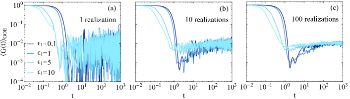
Figure 5: Different number of ensemble realizations in Fig. 2(a). Data for $G(t)$ is averaged over 1, 10, and 100 realizations of GOE.

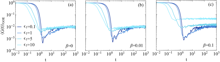
Figure 6: Temperature dependence of $G(t)$ in Fig. 2(a). Data for $G(t)$ is averaged over 100 realizations of GOE with $\beta$=0, 0.01, and 0.1, respectively.

Appendix B The temperature and number of realizations in ensemble average

In the main text, we consider fixed number of realizations and temperature for illustration. In this section, we append Fig. 5 and Fig. 6 to illustrate $G(t)$ with the dependence of the number of realizations and temperature.

References

- Haake [2010] F. Haake, Quantum Signatures of Chaos (Springer, Berlin, 2010).
- Mehta [2004] M. L. Mehta, Random Matrices, 3rd ed. (Elsevier, San Diego, 2004).
- Zelevinsky [1996] V. Zelevinsky, Quantum chaos and complexity in nuclei, Annual Review of Nuclear and Particle Science 46, 237 (1996).
- Guhr et al. [1998] T. Guhr, A. Müller-Groeling, and H. A. Weidenmüller, Random-matrix theories in quantum physics: common concepts, Physics Reports 299, 189 (1998).
- Srednicki [1994] M. Srednicki, Chaos and quantum thermalization, Phys. Rev. E 50, 888 (1994).
- D’Alessio et al. [2016] L. D’Alessio, Y. Kafri, A. Polkovnikov, and M. Rigol, From quantum chaos and eigenstate thermalization to statistical mechanics and thermodynamics, Advances in Physics 65, 239 (2016).
- Hayden and Preskill [2007] P. Hayden and J. Preskill, Black holes as mirrors: quantum information in random subsystems, J. High Energy Phys. 2007 (09), 120.
- Sekino and Susskind [2008] Y. Sekino and L. Susskind, Fast scramblers, J. High Energy Phys. 2008 (10), 065.
- Shenker and Stanford [2014] S. H. Shenker and D. Stanford, Black holes and the butterfly effect, J. High Energy Phys. 2014 (3), 67.
- Maldacena et al. [2016] J. Maldacena, S. H. Shenker, and D. Stanford, A bound on chaos, J. High Energy Phys. 2016 (8), 106.
- Cotler et al. [2017a] J. S. Cotler, G. Gur-Ari, M. Hanada, J. Polchinski, P. Saad, S. H. Shenker, D. Stanford, A. Streicher, and M. Tezuka, Black holes and random matrices, J. High Energy Phys. 2017 (5), 118.
- Franz and Rozali [2018] M. Franz and M. Rozali, Mimicking black hole event horizons in atomic and solid-state systems, Nature Reviews Materials 3, 491 (2018).
- Forrester [2010] P. Forrester, Log-Gases and Random Matrices (LMS-34), London Mathematical Society Monographs (Princeton University Press, 2010).
- Boixo et al. [2018] S. Boixo, S. V. Isakov, V. N. Smelyanskiy, R. Babbush, N. Ding, Z. Jiang, M. J. Bremner, J. M. Martinis, and H. Neven, Characterizing quantum supremacy in near-term devices, Nature Physics 14, 595 (2018).
- Emerson et al. [2002] J. Emerson, Y. S. Weinstein, S. Lloyd, and D. G. Cory, Fidelity decay as an efficient indicator of quantum chaos, Phys. Rev. Lett. 89, 284102 (2002).
- Kowalewska-Kudłaszyk et al. [2009] A. Kowalewska-Kudłaszyk, J. Kalaga, and W. Leoński, Long-time fidelity and chaos for a kicked nonlinear oscillator system, Physics Letters A 373, 1334 (2009).
- Gorin et al. [2006] T. Gorin, T. Prosen, T. H. Seligman, and M. Znidaric, Dynamics of loschmidt echoes and fidelity decay, Physics Reports 435, 33 (2006).
- Larkin and Ovchinnikov [1969] A. I. Larkin and Y. N. Ovchinnikov, Quasiclassical Method in the Theory of Superconductivity, Sov. Phys. JETP 28, 1200 (1969).
- Susskind [2016] L. Susskind, The typical-state paradox: diagnosing horizons with complexity, Fortschritte der Physik 64, 84 (2016).
- Cotler et al. [2017b] J. Cotler, N. Hunter-Jones, J. Liu, and B. Yoshida, Chaos, complexity, and random matrices, J. High Energy Phys. 2017 (11), 48.
- Roberts and Yoshida [2017] D. A. Roberts and B. Yoshida, Chaos and complexity by design, J. High Energy Phys. 2017 (4), 121.
- Chenu et al. [2018] A. Chenu, I. L. Egusquiza, J. Molina-Vilaplana, and A. del Campo, Quantum work statistics, loschmidt echo and information scrambling, Scientific Reports 8, 12634 (2018).
- Kudler-Flam et al. [2020] J. Kudler-Flam, L. Nie, and S. Ryu, Conformal field theory and the web of quantum chaos diagnostics, J. High Energy Phys. 2020 (1), 175.
- Yan et al. [2020] B. Yan, L. Cincio, and W. H. Zurek, Information scrambling and loschmidt echo, Phys. Rev. Lett. 124, 160603 (2020).
- Bhattacharyya et al. [2022] A. Bhattacharyya, W. Chemissany, S. S. Haque, and B. Yan, Towards the web of quantum chaos diagnostics, The European Physical Journal C 82, 1 (2022).
- Karkuszewski et al. [2002] Z. P. Karkuszewski, C. Jarzynski, and W. H. Zurek, Quantum chaotic environments, the butterfly effect, and decoherence, Phys. Rev. Lett. 89, 170405 (2002).
- Poulin et al. [2004] D. Poulin, R. Blume-Kohout, R. Laflamme, and H. Ollivier, Exponential speedup with a single bit of quantum information: Measuring the average fidelity decay, Phys. Rev. Lett. 92, 177906 (2004).
- Syzranov et al. [2018] S. V. Syzranov, A. V. Gorshkov, and V. Galitski, Out-of-time-order correlators in finite open systems, Phys. Rev. B 97, 161114 (2018).
- Xu et al. [2019] Z. Xu, L. P. García-Pintos, A. Chenu, and A. del Campo, Extreme decoherence and quantum chaos, Phys. Rev. Lett. 122, 014103 (2019).
- del Campo and Takayanagi [2020] A. del Campo and T. Takayanagi, Decoherence in Conformal Field Theory, J. High Energy Phys. 2020 (170), 170.
- Tuziemski [2019] J. Tuziemski, Out-of-time-ordered correlation functions in open systems: A feynman-vernon influence functional approach, Phys. Rev. A 100, 062106 (2019).
- Yoshida and Yao [2019] B. Yoshida and N. Y. Yao, Disentangling scrambling and decoherence via quantum teleportation, Phys. Rev. X 9, 011006 (2019).
- Sá et al. [2020a] L. Sá, P. Ribeiro, and T. Prosen, Complex spacing ratios: A signature of dissipative quantum chaos, Phys. Rev. X 10, 021019 (2020a).
- Xu et al. [2021] Z. Xu, A. Chenu, T. Prosen, and A. del Campo, Thermofield dynamics: Quantum chaos versus decoherence, Phys. Rev. B 103, 064309 (2021).
- Zanardi and Anand [2021] P. Zanardi and N. Anand, Information scrambling and chaos in open quantum systems, Phys. Rev. A 103, 062214 (2021).
- Anand et al. [2021] N. Anand, G. Styliaris, M. Kumari, and P. Zanardi, Quantum coherence as a signature of chaos, Phys. Rev. Research 3, 023214 (2021).
- Cornelius et al. [2022] J. Cornelius, Z. Xu, A. Saxena, A. Chenu, and A. del Campo, Spectral filtering induced by non-hermitian evolution with balanced gain and loss: Enhancing quantum chaos, Phys. Rev. Lett. 128, 190402 (2022).
- Borgonovi et al. [2016] F. Borgonovi, F. M. Izrailev, L. F. Santos, and V. G. Zelevinsky, Quantum chaos and thermalization in isolated systems of interacting particles, Physics Reports 626, 1 (2016).
- Leviandier et al. [1986] L. Leviandier, M. Lombardi, R. Jost, and J. P. Pique, Fourier transform: A tool to measure statistical level properties in very complex spectra, Phys. Rev. Lett. 56, 2449 (1986).
- Wilkie and Brumer [1991] J. Wilkie and P. Brumer, Time-dependent manifestations of quantum chaos, Phys. Rev. Lett. 67, 1185 (1991).
- Alhassid and Whelan [1993] Y. Alhassid and N. Whelan, Onset of chaos and its signature in the spectral autocorrelation function, Phys. Rev. Lett. 70, 572 (1993).
- Ma [1995] J.-Z. Ma, Correlation hole of survival probability and level statistics, Journal of the Physical Society of Japan 64, 4059 (1995).
- Dyer and Gur-Ari [2017] E. Dyer and G. Gur-Ari, 2d cft partition functions at late times, J. High Energy Phys. 2017 (8), 75.
- del Campo et al. [2017] A. del Campo, J. Molina-Vilaplana, and J. Sonner, Scrambling the spectral form factor: Unitarity constraints and exact results, Phys. Rev. D 95, 126008 (2017).
- Joshi et al. [2022] L. K. Joshi, A. Elben, A. Vikram, B. Vermersch, V. Galitski, and P. Zoller, Probing many-body quantum chaos with quantum simulators, Phys. Rev. X 12, 011018 (2022).
- Srivastava et al. [2016] S. C. L. Srivastava, S. Tomsovic, A. Lakshminarayan, R. Ketzmerick, and A. Bäcker, Universal scaling of spectral fluctuation transitions for interacting chaotic systems, Phys. Rev. Lett. 116, 054101 (2016).
- Prakash and Lakshminarayan [2020] R. Prakash and A. Lakshminarayan, Scrambling in strongly chaotic weakly coupled bipartite systems: Universality beyond the ehrenfest timescale, Phys. Rev. B 101, 121108 (2020).
- Styliaris et al. [2021] G. Styliaris, N. Anand, and P. Zanardi, Information scrambling over bipartitions: Equilibration, entropy production, and typicality, Phys. Rev. Lett. 126, 030601 (2021).
- Can [2019] T. Can, Random lindblad dynamics, Journal of Physics A: Mathematical and Theoretical 52, 485302 (2019).
- Denisov et al. [2019] S. Denisov, T. Laptyeva, W. Tarnowski, D. Chruściński, and K. Życzkowski, Universal spectra of random lindblad operators, Phys. Rev. Lett. 123, 140403 (2019).
- Sá et al. [2020b] L. Sá, P. Ribeiro, T. Can, and T. Prosen, Spectral transitions and universal steady states in random kraus maps and circuits, Phys. Rev. B 102, 134310 (2020b).
- Tarnowski et al. [2021] W. Tarnowski, I. Yusipov, T. Laptyeva, S. Denisov, D. Chruściński, and K. Życzkowski, Random generators of markovian evolution: A quantum-classical transition by superdecoherence, Phys. Rev. E 104, 034118 (2021).
- Sá et al. [2022] L. Sá, P. Ribeiro, and T. Prosen, Lindbladian dissipation of strongly-correlated quantum matter, Phys. Rev. Research 4, L022068 (2022).
- Livan et al. [2018] G. Livan, M. Novaes, and P. Vivo, Introduction to Random Matrices: Theory and Practice (Springer, 2018).
- Maldacena and Qi [2018] J. Maldacena and X.-L. Qi, Eternal traversable wormhole, (2018), arXiv:1804.00491 [hep-th] .
- Chen et al. [2017] X. Chen, R. Fan, Y. Chen, H. Zhai, and P. Zhang, Competition between chaotic and nonchaotic phases in a quadratically coupled sachdev-ye-kitaev model, Phys. Rev. Lett. 119, 207603 (2017).
- Song et al. [2017] X.-Y. Song, C.-M. Jian, and L. Balents, Strongly correlated metal built from sachdev-ye-kitaev models, Phys. Rev. Lett. 119, 216601 (2017).
- Jian and Yao [2017] S.-K. Jian and H. Yao, Solvable sachdev-ye-kitaev models in higher dimensions: From diffusion to many-body localization, Phys. Rev. Lett. 119, 206602 (2017).
- García-García et al. [2019] A. M. García-García, T. Nosaka, D. Rosa, and J. J. M. Verbaarschot, Quantum chaos transition in a two-site sachdev-ye-kitaev model dual to an eternal traversable wormhole, Phys. Rev. D 100, 026002 (2019).
- Plugge et al. [2020] S. Plugge, E. Lantagne-Hurtubise, and M. Franz, Revival dynamics in a traversable wormhole, Phys. Rev. Lett. 124, 221601 (2020).
- Qi and Zhang [2020] X.-L. Qi and P. Zhang, The coupled syk model at finite temperature, J. High Energy Phys. 2020 (5), 129.
- Sahoo et al. [2020] S. Sahoo, E. Lantagne-Hurtubise, S. Plugge, and M. Franz, Traversable wormhole and hawking-page transition in coupled complex syk models, Phys. Rev. Research 2, 043049 (2020).
- Haenel et al. [2021] R. Haenel, S. Sahoo, T. H. Hsieh, and M. Franz, Traversable wormhole in coupled sachdev-ye-kitaev models with imbalanced interactions, Phys. Rev. B 104, 035141 (2021).
- Zhou et al. [2021] T.-G. Zhou, L. Pan, Y. Chen, P. Zhang, and H. Zhai, Disconnecting a traversable wormhole: Universal quench dynamics in random spin models, Phys. Rev. Research 3, L022024 (2021).
- Xu and del Campo [2019] Z. Xu and A. del Campo, Probing the full distribution of many-body observables by single-qubit interferometry, Phys. Rev. Lett. 122, 160602 (2019).
- Poulin et al. [2003] D. Poulin, R. Laflamme, G. J. Milburn, and J. P. Paz, Testing integrability with a single bit of quantum information, Phys. Rev. A 68, 022302 (2003).
- Emerson et al. [2004] J. Emerson, S. Lloyd, D. Poulin, and D. Cory, Estimation of the local density of states on a quantum computer, Phys. Rev. A 69, 050305(R) (2004).
- Quan et al. [2006] H. T. Quan, Z. Song, X. F. Liu, P. Zanardi, and C. P. Sun, Decay of loschmidt echo enhanced by quantum criticality, Phys. Rev. Lett. 96, 140604 (2006).
- Zhang et al. [2008] J. Zhang, X. Peng, N. Rajendran, and D. Suter, Detection of quantum critical points by a probe qubit, Phys. Rev. Lett. 100, 100501 (2008).
- Dorner et al. [2013] R. Dorner, S. R. Clark, L. Heaney, R. Fazio, J. Goold, and V. Vedral, Extracting quantum work statistics and fluctuation theorems by single-qubit interferometry, Phys. Rev. Lett. 110, 230601 (2013).
- Mazzola et al. [2013] L. Mazzola, G. De Chiara, and M. Paternostro, Measuring the characteristic function of the work distribution, Phys. Rev. Lett. 110, 230602 (2013).
- Batalhão et al. [2014] T. B. Batalhão, A. M. Souza, L. Mazzola, R. Auccaise, R. S. Sarthour, I. S. Oliveira, J. Goold, G. De Chiara, M. Paternostro, and R. M. Serra, Experimental reconstruction of work distribution and study of fluctuation relations in a closed quantum system, Phys. Rev. Lett. 113, 140601 (2014).
- Wei and Liu [2012] B.-B. Wei and R.-B. Liu, Lee-yang zeros and critical times in decoherence of a probe spin coupled to a bath, Phys. Rev. Lett. 109, 185701 (2012).
- Peng et al. [2015] X. Peng, H. Zhou, B.-B. Wei, J. Cui, J. Du, and R.-B. Liu, Experimental observation of lee-yang zeros, Phys. Rev. Lett. 114, 010601 (2015).
- Francis et al. [2021] A. Francis, D. Zhu, C. Huerta Alderete, S. Johri, X. Xiao, J. K. Freericks, C. Monroe, N. M. Linke, and A. F. Kemper, Many-body thermodynamics on quantum computers via partition function zeros, Science Advances 7, 2447 (2021).
- Swingle et al. [2016] B. Swingle, G. Bentsen, M. Schleier-Smith, and P. Hayden, Measuring the scrambling of quantum information, Phys. Rev. A 94, 040302 (2016).
- Liu et al. [2019] Y. Liu, J. Tian, R. Betzholz, and J. Cai, Pulsed quantum-state reconstruction of dark systems, Phys. Rev. Lett. 122, 110406 (2019).
- Vasilyev et al. [2020] D. V. Vasilyev, A. Grankin, M. A. Baranov, L. M. Sieberer, and P. Zoller, Monitoring quantum simulators via quantum nondemolition couplings to atomic clock qubits, PRX Quantum 1, 020302 (2020).
- Papadodimas and Raju [2015] K. Papadodimas and S. Raju, Local operators in the eternal black hole, Phys. Rev. Lett. 115, 211601 (2015).
- Chenu et al. [2019] A. Chenu, J. Molina-Vilaplana, and A. del Campo, Work Statistics, Loschmidt Echo and Information Scrambling in Chaotic Quantum Systems, Quantum 3, 127 (2019).
- Liu [2018] J. Liu, Spectral form factors and late time quantum chaos, Phys. Rev. D 98, 086026 (2018).
- Liu et al. [2017] Y. Liu, M. A. Nowak, and I. Zahed, Disorder in the sachdev-ye-kitaev model, Physics Letters B 773, 647 (2017).
- Hunter-Jones and Liu [2018] N. Hunter-Jones and J. Liu, Chaos and random matrices in supersymmetric syk, J. High Energy Phys. 2018 (5), 202.
- Tkocz et al. [2012] T. Tkocz, M. Smaczyński, M. Kuś, O. Zeitouni, and K. Życzkowski, Tensor products of random unitary matrices, Random Matrices: Theory and Applications 01, 1250009 (2012).
- Sachdev and Ye [1993] S. Sachdev and J. Ye, Gapless spin-fluid ground state in a random quantum heisenberg magnet, Phys. Rev. Lett. 70, 3339 (1993).
- [86] A. Kitaev, A simple model of quantum holography,, Talks at The KITP on April 7 and May 27, 2015.
- Liao and Galitski [2022] Y. Liao and V. Galitski, Universal dephasing mechanism of many-body quantum chaos, Phys. Rev. Research 4, L012037 (2022).
- Danshita et al. [2017] I. Danshita, M. Hanada, and M. Tezuka, Creating and probing the Sachdev-Ye-Kitaev model with ultracold gases: Towards experimental studies of quantum gravity, Progress of Theoretical and Experimental Physics 2017 (2017), 083I01.
- García-Álvarez et al. [2017] L. García-Álvarez, I. L. Egusquiza, L. Lamata, A. del Campo, J. Sonner, and E. Solano, Digital quantum simulation of minimal , Phys. Rev. Lett. 119, 040501 (2017).
- Pikulin and Franz [2017] D. I. Pikulin and M. Franz, Black hole on a chip: Proposal for a physical realization of the sachdev-ye-kitaev model in a solid-state system, Phys. Rev. X 7, 031006 (2017).
- Chew et al. [2017] A. Chew, A. Essin, and J. Alicea, Approximating the sachdev-ye-kitaev model with majorana wires, Phys. Rev. B 96, 121119 (2017).
- Luo et al. [2019] Z. Luo, Y.-Z. You, J. Li, C.-M. Jian, D. Lu, C. Xu, B. Zeng, and R. Laflamme, Quantum simulation of the non-fermi-liquid state of sachdev-ye-kitaev model, npj Quantum Information 5, 53 (2019).
- Babbush et al. [2019] R. Babbush, D. W. Berry, and H. Neven, Quantum simulation of the sachdev-ye-kitaev model by asymmetric qubitization, Phys. Rev. A 99, 040301 (2019).
- Wei and Sedrakyan [2021] C. Wei and T. A. Sedrakyan, Optical lattice platform for the sachdev-ye-kitaev model, Phys. Rev. A 103, 013323 (2021).