MonoPLFlowNet: Permutohedral Lattice FlowNet for Real-Scale 3D Scene Flow Estimation with Monocular Images

Abstract

Real-scale scene flow estimation has become increasingly important for 3D computer vision. Some works successfully estimate real-scale 3D scene flow with LiDAR. However, these ubiquitous and expensive sensors are still unlikely to be equipped widely for real application. Other works use monocular images to estimate scene flow, but their scene flow estimations are normalized with scale ambiguity, where additional depth or point cloud ground truth are required to recover the real scale. Even though they perform well in 2D, these works do not provide accurate and reliable 3D estimates. We present a deep learning architecture on permutohedral lattice - MonoPLFlowNet. Different from all previous works, our MonoPLFlowNet is the first work where only two consecutive monocular images are used as input, while both depth and 3D scene flow are estimated in real scale. Our real-scale scene flow estimation outperforms all state-of-the-art monocular-image based works recovered to real scale by ground truth, and is comparable to LiDAR approaches. As a by-product, our real-scale depth estimation also outperforms other state-of-the-art works. Code will be available at https://github.com/BlarkLee/MonoPLFlowNet.

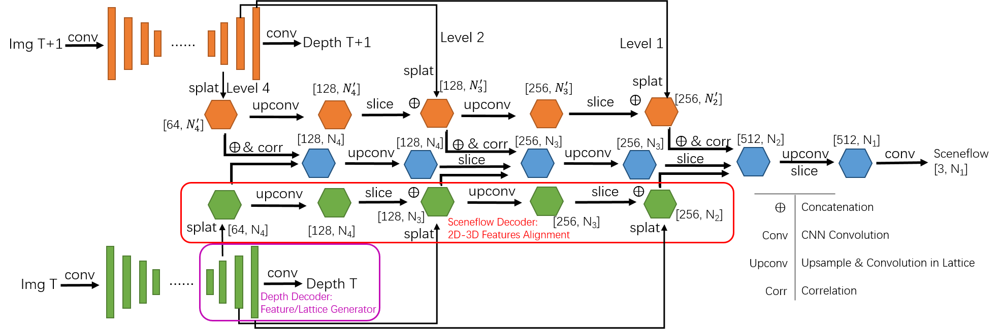
Figure 2: MonoPLFlowNet Architecture: An Hour-Glass like encoder-decoder based network. It shares the same encoder for two monocular images as the only input, and jointly estimates the depth and 3D scene flow in real scale by decoding separately with a Depth decoder (purple box) and a Sceneflow Decoder (red box). Architectures of the two decoders are shown in Figure 3 and 4, respectively.

1 Introduction

Scene flow are 3D vectors associating the corresponding 3D point-wise motion between consecutive frames, where scene flow can be recognized as lifting up pixel-wise 2D optical flow from the image plane to 3D space. Different to coarsely high-level motion cues such as bounding-box based tracking, 3D scene flow focuses on precisely low-level point-wise motion cues. With such advantage, scene flow can either serve for non-rigid motion as visual odometry and ego motion estimation, or rigid motion as multi-object tracking, which makes it increasingly important in motion perception/segmentation and applications in dynamic environments such as robotics, autonomous driving and human-computer interaction.

3D scene flow has been widely studied using LiDAR point cloud [27, 44, 40, 3, 15, 46, 34] from two consecutive frames as input, where a few recent LiDAR works achieve very accurate performances. However, LiDARs are still too expensive to be equipped for real applications. Other sensors are also being explored for 3D scene flow estimation such as RGB-D cameras [29, 16, 20] and stereo cameras[42, 39, 2, 22, 30]. However, each sensor configuration also has its own limitation, such as RGB-D cameras are only reliable in the indoor environment, while stereo cameras require calibration for stereo rigs.

Since Monocular camera is ubiquitous and cheap for all real applications, it is a promising alternative to the complicated and expensive sensors. There are many works for monocular image-based scene flow estimation[52, 54, 37, 8, 50, 28, 48, 18, 19], where CNN models are designed to jointly estimate monocular depth and optical/scene flow. However, their estimations are all with scale ambiguity. This problem exists in all monocular works where they estimate normalized depth and optical/scene flow. To recover to the real scale, they require depth and scene flow ground truth, which are possible to obtain for evaluation in labeled datasets but impossible for a real application.

Our motivation for this work is to take the advantages and overcome the limitations from both LiDAR-based (real-scale, accurate but expensive) and image-based (cheap, ubiquitous but scale-ambiguous) approaches. Our key contributions are:

• We build a deep learning architecture MonoPLFlowNet, which is the first work using only two consecutive monocular images to estimate in real scale both the depth and 3D scene flow.

• Our 3D scene flow estimation outperforms all state-of-the-art monocular image-based works even after recovering their scale ambiguities with ground truth, and is comparable to LiDAR-based approaches.

• We introduce a novel method - ”Pyramid-Level 2D-3D features alignment between Cartesian Coordinate and Permutohedral Lattice Network”, which bridges the gap between features in monocular images and 3D points in our application, and inspires a new way to align 2D-3D information for computer vision tasks which could benefit other applications.

• As a byproduct, our linear-additive depth estimation from MonoPLFlowNet also outperforms state-of-the-art works on monocular depth estimation.

2 Related Works

Monocular image-based scene flow estimation: Monocular 3D scene flow estimation originates from 2D optical flow estimation[9, 48]. To get real-scale 3D scene flow from 2D optical flow, real-scale 3D coordinates are required which could be derived from real-scale depth map. Recently, following the success from SFM (Structure from Motion) [47, 25], many works jointly estimate monocular depth and 2D optical flow [52, 54, 37, 8, 50, 28]. However, as seen in most SFM models, the real scale decays in jointly training and leads to scale ambiguity. Although [18, 19] jointly estimate depth and 3D scene flow directly, they suffer from scale ambiguity, which is the biggest issue for monocular image-based approaches.

3D Point cloud based scene flow estimation: Following PointNet[6] and PointNet++[36], it became possible to use CNN-based models to directly process point cloud for different tasks including 3D scene flow estimation. Since directly implementing on 3D points, there is no scale ambiguity. The success of CNN-based 2D optical flow networks also boost 3D scene flow. FlowNet3D[27] builds on PointNet++ and imitates the process used in 2D optical FlowNet[9] to build a 3D correlation layer. PointPWC-net[46] imitates another 2D optical flow network PWC-net[41] to build 3D cost volume layers. The most successful works are ”Permutohedral Lattice family”, where BCL[21], SplatNet[40], HPLFlowNet[15], PointFlowNet[3] all belong to the family. The lattice (more details will be provided in Section 3.1) is a very efficient representation for processing of high-dimensional data [1], including 3D point cloud. Point cloud based methods achieves better performance than image-based methods. However, with LiDAR scanning as the input, they are still too expensive for real applications.

Our MonoPLFlowNet takes advantages and overcome limitations from both image (cheap, ubiquitous but scale-ambiguous) and LiDAR (real-scale, accurate but expensive) based approaches by only using monocular images to jointly estimate depth and 3D scene flow in real scale.

3 MonoPLFlowNet

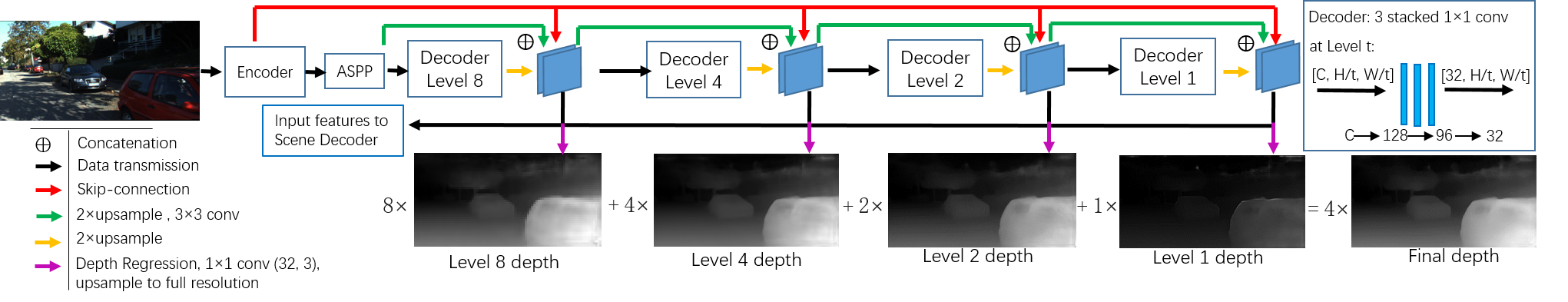
Figure 3: Depth Decoder: Pyramid-Level Linearly-Additive Depth Estimation. Besides the accurate depth estimation, from a whole architecture view, our depth decoder also serves as the feature/lattice position generator, which is why we design it in linear-additive way.

Our MonoPLFlowNet is an hour-glass encoder-decoder based model, which only takes two consecutive monocular images as input, while both the depth and 3D scene flow are estimated in real scale. Figure 2 shows our network architecture. While sharing the same encoder, we use separate decoders for depth and scene flow. With our designed mechanism, we align the 2D-3D features to boost the performance of each other. In this section, we present the theory of permutohedral lattice, and then discuss how we design and align the two decoders.

3.1 Review of Permutohedral Lattice Filtering

High-Dimensional Gaussian Filtering: Signal’s value and position are two important aspects of filtering. Eq. 1 shows a general form of high-dimensional Gaussian filtering:

$$\vec{v_{i}}=\sum_{j=1}^{n}exp^{-\frac{1}{2}(\vec{p_{i}}-\vec{p_{j}})^{T}\sum^{-1}(\vec{p_{i}}-\vec{p_{j}})^{T}}\vec{v_{j}}$$ (1)

$$\vec{v_{i}}=(r_{i},g_{i},b_{i},1),\;\vec{p_{i}}=(\frac{x_{i}}{\sigma_{s}},\frac{y_{i}}{\sigma_{s}})$$ (2)

$$\vec{v_{i}}=(r_{i},g_{i},b_{i},1),\;\vec{p_{i}}=(\frac{x_{i}}{\sigma_{s}},\frac{y_{i}}{\sigma_{s}},\frac{I_{i}}{\sigma_{c}})$$ (3)

$$\vec{v_{i}}=(r_{i},g_{i},b_{i},1),\;\vec{p_{i}}=(\frac{x_{i}}{\sigma_{s}},\frac{y_{i}}{\sigma_{s}},\frac{r_{i}}{\sigma_{c}},\frac{g_{i}}{\sigma_{c}},\frac{b_{i}}{\sigma_{c}})$$ (4)

where $exp^{-\frac{1}{2}(\vec{p_{i}}-\vec{p_{j}})^{T}\sum^{-1}(\vec{p_{i}}-\vec{p_{j}})^{T}}$ is a Gaussian distribution denoting the weight of the neighbor signal value $\vec{v_{j}}$ contributing to the target signal $\vec{v_{i}}$. Here $\vec{v}$ is the value vector of the signal, and $\vec{p}$ is the position vector of the signal. Equation 2, 3 and 4 denote Gaussian blur filter, gray-scale bilateral filter and color bilateral filter, respectively, where $v_{i}$ and $p_{i}$ are defined in Eq. 1. For these image filters, the signals are pixels, the signal values are 3D homogeneous color space, and signal positions are 2D, 3D and 5D, respectively, and the filtering processing is on 2D image Cartesian coordinate. The dimension of the position vector can be extended to $d$, which is called a d-dimensional Gaussian filter. We refer the readers to [1, 21] and our supplementary materials for more details.

Permutohedral Lattice Network: However, a high-dimensional Gaussian filter can be also implemented on features with $n$ dimension rather than on pixels with 3D color space. The filtering process can be implemented in a more efficient space, the Permutohedral Lattice rather than a traditional Cartesian 2D image plane or 3D space. The $d$-dimensional permutohedral lattice is defined as the projection of the scaled Cartesian $(d+1)$-dimensional grid along the vector $\vec{1}=[1,1...1]$ onto the hyperplane $H_{d}$, which is the subspace of $R_{d+1}$ in which coordinates sum to zero:

$$B_{d}=\begin{bmatrix}d&-1&...&-1\\ -1&d&...&-1\\ ...&...&...&...\\ -1&-1&...&d\end{bmatrix}$$ (5)

Therefore it is also spanned by the projection of the standard basis for the original $(d+1)$-dimensional Cartesian space to $H_{d}$. In other words, we can project a feature at Cartesian coordinate $p_{cart}$ to Permutohedral Lattice coordinate $p_{lat}$ as:

$$\vec{p_{lat}}={B_{d}}\vec{p_{cart}}$$ (6)

With features embedding on lattice, [1] derived a maneuver pipeline “splatting-convolution-slicing” for feature processing in lattice; [21] improved the pipeline to be learnable BCL (Bilateral Convolutional Layers). Following CNN notion, [15] improved BCL to different levels of receptive fields.

To summarize, Permutohedral Lattice Network convolves the feature values $\vec{v_{i}}$ based on feature positions $\vec{p_{i}}$. While it is straightforward to derive $\vec{v_{i}}$ and $\vec{p_{i}}$ when feature positions and lattice have equal dimension, eg. 3D Lidar points input to 3D lattice[21, 40, 15] or 2D to 2D [45, 1], it is challenging when dimensions are different, as in the case of our 2D image input to 3D lattice. The proposed MonoPLFlowNet is designed to overcome such problem.

3.2 Depth Decoder

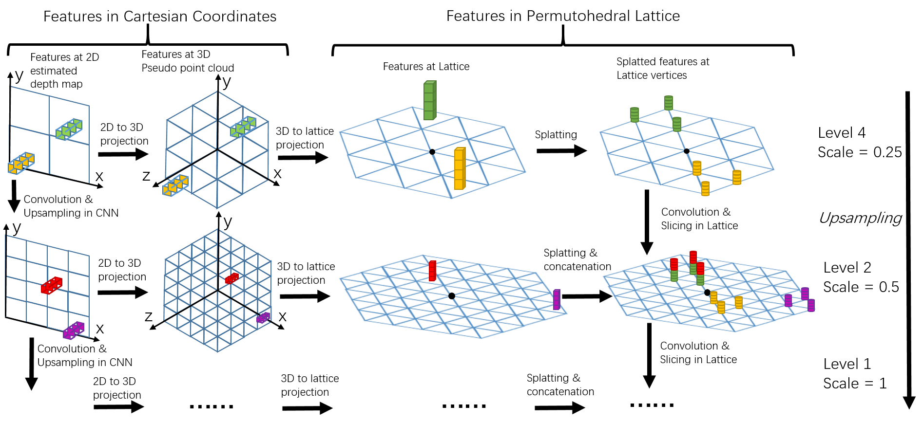
Figure 4: 3D Scene Flow Decoder: Pyramid-Level 2D-3D features alignment between Cartesian Coordinate and Permutohedral Lattice Network. Horizontally it shows the feature embedding from Cartesian coordinate to permutohedral lattice. Vertically, it shows how the features are upsampled and concatenated for the next level.

We design our depth module as an encoder-decoder based network as shown in Figure 3. Following the success of BTS DepthNet[24], we use their same encoder as a CNN-based feature extractor followed by the dilated convolution (ASPP)[49, 7]. Our major contribution focuses on the decoder from three aspects.

Level-Based Decoder: First, while keeping a pyramid-level top-down reasoning, BTS designed “lpg” (local planar guidance) to regress depth at each level. In our experiments, we found that “lpg” is a block where accuracy is sacrificed for efficiency. Instead, we replace the “lpg” with our “level-based decoder” as shown in Fig. 3, and improve the decoder to accommodate our sceneflow task.

Pyramid-Level Linearly-Additive mechanism: BTS concatenates the estimated depth at each level and uses a final convolution to regress the final depth in a non-linear way, implying that the estimated depth at each level is not in a fixed scale. Instead, we propose a “Pyramid-Level Linearly-Additive mechanism” as:

$$d_{final}=\frac{1}{4}(1\times d_{lev1}+2\times d_{lev2}+4\times d_{lev4}+8\times d_{lev8})$$ (7)

such that the final estimation is a linear combination over each level depth, where we force $d_{lev1}$, $d_{lev2}$, $d_{lev4}$, $d_{lev8}$ to be in $1,\frac{1}{2},\frac{1}{4},\frac{1}{8}$ scale of the real-scale depth. In order to achieve this, we also need to derive a pyramid-level loss corresponding to the level of the decoder architecture to supervise the depth at each level as Eq. 11.

Experiments show that with our improvement, our depth decoder outperforms the baseline BTS as well as other state-of-the-art works. More importantly, the objective is to design the depth decoder to generate feature/lattice for the scene flow decoder, which is our major contribution. More detail is provided in the next section.

3.3 Scene Flow Decoder

Our scene flow decoder is designed as a two-stream pyramid-level model which decodes in parallel in two domains - 2D Cartesian coordinate and 3D permutalhedral lattice, as shown in Figure 4. As mentioned in Section 3.1, feature values and positions are two key factors in filtering processing. For the feature values, we use the features decoded by level-based decoder from depth module as shown in Figure 3, the features as the input to scene decoder (32 dimensions) are before regressing to the corresponding level depth (purple arrow), which means the input features to the scene decoder are the high-level feature representation of the corresponding level depth. While values are trivial, positions are not straightforward. As the challenge mentioned in Section 3.1, the 2D feature position from our depth is not enough to project the feature values to 3D permutohedral lattice. We derive a novel strategy to overcome this challenge by projecting the estimated depth estimation into 3D space to generate real-scale pseudo point cloud. Since pseudo point cloud has real-scale 3D coordinates, we can project the feature values from the 2D depth map to 3D point cloud in Cartesian coordinate, and then project to the corresponding position in 3D permutohedral lattice. A 2D to 3D projection is defined as:

Method	Output	Scale	higher is better			lower is better
			$\delta<$ 1.25	$\delta<$ 1.25	$\delta<$ 1.25	Abs Rel	Sq Rel	RMSE	RMSE log
Make3D[38]	D	✓	0.601	0.820	0.926	0.280	3.012	8.734	0.361
Eigen et al.[10]	D	✓	0.702	0.898	0.967	0.203	1.548	6.307	0.282
Liu et al.[26]	D	✓	0.680	0.898	0.967	0.201	1.584	6.471	0.273
LRC (CS + K)[14]	D	✓	0.861	0.949	0.976	0.114	0.898	4.935	0.206
Kuznietsov et al.[23]	D	✓	0.862	0.960	0.986	0.113	0.741	4.621	0.189
Gan et al.[12]	D	✓	0.890	0.964	0.985	0.098	0.666	3.933	0.173
DORN[11]	D	✓	0.932	0.984	0.994	0.072	0.307	2.727	0.120
Yin et al.[51]	D	✓	0.938	0.990	0.998	0.072	-	3.258	0.117
BTS (DenseNet-121)[24]	D	✓	0.951	0.993	0.998	0.063	0.256	2.850	0.100
BTS (ResNext-101)[24]	D	✓	0.956	0.993	0.998	0.059	0.245	2.756	0.096
GeoNet[52]	D + 2DF	✗	0.793	0.931	0.973	0.155	1.296	5.857	0.233
DFNet[54]	D + 2DF	✗	0.818	0.943	0.978	0.146	1.182	5.215	0.213
CC[37]	D + 2DF	✗	0.826	0.941	0.975	0.140	1.070	5.326	0.217
GLNet[8]	D + 2DF	✗	0.841	0.948	0.980	0.135	1.070	5.230	0.210
EPC[50]	D + 2DF	✗	0.847	0.926	0.969	0.127	1.239	6.247	0.214
EPC++[28]	D + 2DF	✗	0.841	0.946	0.979	0.127	0.936	5.008	0.209
Mono-SF[18]	D + 3DF	✗	0.851	0.950	0.978	0.125	0.978	4.877	0.208
Ours (DenseNet-121)	D + 3DF	✓	0.960	0.994	0.999	0.060	0.230	2.627	0.095

Table 1: Monocular depth results comparison on KITTI Eigen’s split. In the column Output, D denotes depth, 2DF and 3DF denote 2D optical flow and 3D scene flow. In the column Scale, ✓denotes in real scale, ✗ denotes with scale ambiguity. DenseNet-121 as backbone for efficiency.

$$\begin{bmatrix}x\\ y\\ z\end{bmatrix}=\begin{bmatrix}{z}/{f_{u}}&0&{-c_{u}}z/{f_{u}}\\ 0&{z}/{f_{v}}&{-c_{v}}z/{f_{v}}\\ 0&0&z\end{bmatrix}\begin{bmatrix}u\\ v\\ 1\end{bmatrix}$$ (8)

where $z$ is the estimated depth, $(u,v)$ is the corresponding pixel coordinate in the depth map, $f_{u},f_{v}$ are horizontal and vertical camera focal lengths, $(c_{u},c_{v})$ are the coordinate of camera principle point. $(x,y,z)$ is the coordinate of the projected 3D point.

So far we have successfully derived the projection in the real scale, where the complete projection pipeline consisting of 2D to 3D (Eq. 8) and 3D to lattice (Eq. 6) is shown in Figure 4. Due to the linear property of the projection, the proposed projection pipeline holds at different scales in the overall system. Using this property, we prove a stronger conclusion: scaling the feature depth from Cartesian coordinate leads to a same scale to the corresponding feature position in permutohedral lattice. Eq. 9 summarizes the mapping where $(p_{x},p_{y},p_{z})$ is the permutohedral lattice coordinate of the feature corresponding to its 2D Cartisian coordinate in the depth map.

$$\begin{split}\begin{bmatrix}p^{\prime}_{x}\\ p^{\prime}_{y}\\ p^{\prime}_{z}\end{bmatrix}=B_{d}\begin{bmatrix}x^{\prime}\\ y^{\prime}\\ z^{\prime}\end{bmatrix}\\ =B_{d}\begin{bmatrix}{z^{\prime}}/{f^{\prime}_{u}}&0&{-c^{\prime}_{u}}z^{\prime}/{f^{\prime}_{u}}\\ 0&{z^{\prime}}/{f^{\prime}_{v}}&{-c^{\prime}_{u}}z^{\prime}/{f^{\prime}_{u}}\\ 0&0&z^{\prime}\end{bmatrix}\begin{bmatrix}u^{\prime}\\ v^{\prime}\\ 1\end{bmatrix}\\ =B_{d}\begin{bmatrix}{\lambda z}/{\lambda f_{u}}&0&{-\lambda c_{u}}\lambda z/{\lambda f_{u}}\\ 0&{\lambda z}/{\lambda f_{v}}&{-\lambda c_{u}}\lambda z/{\lambda f_{u}}\\ 0&0&\lambda z\end{bmatrix}\begin{bmatrix}u^{\prime}\\ v^{\prime}\\ 1\end{bmatrix}\\ =B_{d}\begin{bmatrix}{z}/{f_{u}}&0&{-c_{u}}\lambda z/{f_{u}}\\ 0&{z}/{f_{v}}&{-c_{u}}\lambda z/{f_{u}}\\ 0&0&\lambda z\end{bmatrix}\begin{bmatrix}\lambda u\\ \lambda v\\ 1\end{bmatrix}\\ =B_{d}\begin{bmatrix}{\lambda z}/{f_{u}}&0&{-c_{u}}\lambda z/{f_{u}}\\ 0&{\lambda z}/{f_{v}}&{-c_{u}}\lambda z/{f_{u}}\\ 0&0&\lambda z\end{bmatrix}\begin{bmatrix}u\\ v\\ 1\end{bmatrix}\\ \end{split}$$ (9)

$B_{d}$ is defined in Eq. 5, $\lambda$ is the scale, a “prime” sign denotes scaling the original value with $\lambda$. Comparing the final result of Eq. 9 to Eq. 8, the only difference is to replace $z$ with $\lambda z$, hence only scaling the depth in Cartesian coordinate will lead to a same scale to the position in permutohedral lattice. Using the proposed “Pyramid-Level 2D-3D features alignment” mechanism, we can embed the features from 2D Cartesian coordinate to 3D Permutohetral lattice, and then implement splating-convolution-slicing and concatenate different level features directly in the permutohedral lattice network. Please see the supplementary materials for more explanation. For the basic operations in permutohedral lattice, we directly refer to [15].

3.4 Loss

Method	Train on	Scale	higher is better			lower is better
			$\delta<$ 1.25	$\delta<$ 1.25	$\delta<$ 1.25	Abs Rel	Sq Rel	RMSE	RMSE log
Mono-SF[18]	K	✗	0.259	0.483	0.648	0.943	19.250	14.676	0.667
Mono-SF-Multi[19]	K	✗	0.273	0.492	0.650	0.931	19.072	14.566	0.666
Ours	F	✓	0.715	0.934	0.980	0.188	1.142	4.400	0.235

Table 2: Monocular depth results comparison on Flyingthings3D dataset. In the column Train on, K denotes KITTI, F denotes Flyingthings3D. In the column Scale, ✓denotes in real scale, ✗ denotes with scale ambiguity.

Method	Train on	Scale	EPE3D(m)	ACC3DS	ACC3DR	Outlier3D	EPE2D(px)	ACC2D
Mono-SF[18]	K	✗	1.1288	0.0525	0.1017	0.9988	58.2761	0.2362
Mono-SF-Multi [19]	K	✗	1.5864	0.0020	0.0050	0.9988	48.3099	0.3162
Ours	F	✓	0.3915	0.5424	0.6911	0.8279	22.4226	0.6659

Table 3: Monocular 3D scene flow results comparison on Flyingthings3D dataset.(image based evaluation standard) In the column Train on, K denotes KITTI, F denotes Flyingthings3D. In the column Scale, ✓denotes in real scale, ✗ denotes with scale ambiguity.

Method	Train on	Scale	EPE3D(m)	ACC3DS	ACC3DR	Outlier3D	EPE2D(px)	ACC2D
[18]depth + Mono-Exp[48]	K	✗	2.7079	0.0676	0.1467	0.9982	181.0699	0.2777
Our depth + Mono-Exp[48]	K	✗	1.6673	0.0838	0.1815	0.9953	78.7245	0.2837
Mono-SF[18]	K	✗	1.1288	0.0525	0.1017	0.9988	58.2761	0.2362
Mono-SF-Multi[19]	K	✗	0.7828	0.1725	0.2548	0.9477	35.9015	0.4886
Ours	F	✓	0.6970	0.2453	0.3692	0.8630	33.4750	0.4968

Table 4: Monocular 3D scene flow results comparison on KITTI flow 2015 dataset.(image based evaluation standard) In the column Train on, K denotes KITTI, F denotes Flyingthings3D. In the column Scale, ✓denotes in real scale, ✗ denotes with scale ambiguity.

Method	EPE3D(m)	Scale	ACC3DS	ACC3DR	Outlier3D	EPE2D(px)	ACC2D
MonoPLFlowNet-lev1	0.4781	✓	0.4587	0.6146	0.8935	26.3133	0.6092
MonoPLFlowNet-lev1-lev2	0.4439	✓	0.4689	0.6333	0.8605	24.3198	0.6366
MonoPLFlowNet-full	0.4248	✓	0.5099	0.6611	0.8595	23.7657	0.6456

Table 5: Ablation study on our MonoPLFlowNet by changing level of the scene decoder.(image based evaluation standard) lev1 denotes only using the last level, lev1-lev2 denotes using the last two levels, full denotes using all levels. For fair comparison, we show all results after training epoch 22.

Depth Loss: Silog (scale-invariant log) loss is a widely-used loss[10] for depth estimation supervision defined as:

$$L_{silog}(\tilde{d},d)=\alpha\sqrt{\frac{1}{T}\sum_{i}(g_{i})^{2}-\frac{\lambda}{T^{2}}(\sum_{i}g_{i})^{2}}\vspace{-2mm}$$ (10)

where $g_{i}=\log\tilde{d_{i}}-\log d_{i}$, $\tilde{d}$ and $d$ are estimated and ground truth depths, $T$ is the number of valid pixels, $\lambda$ and $\alpha$ are constants set to be 0.85 and 10. Since our depth decoder decodes a fixed-scale depth at each level, we do not directly supervise on final depth. Instead, we design a pyramid-level silog loss corresponding to our depth decoder to supervise the estimation from each level.

$$L_{depth}=\frac{1}{15}(8\times L_{1}+4\times L_{2}+2\times L_{4}+1\times L_{8})\vspace{-2mm}$$ (11)

where $L_{level}=L_{silog}(\tilde{d}_{level},d_{level}/n)$. Higher weight is assigned to low-level loss to stabilize the training process.

Scene Flow Loss: Following most LiDAR-based work, we first use a traditional End Point Error (EPE3D) loss as $L_{epe}=||\tilde{sf}-sf||_{2}$, where $\tilde{sf}$ and $sf$ are estimated and ground truth scene flows, respectively. To bring two sets of point clouds together, some self-supervised works leverage the Chamfer distance loss as:

$$L_{cham}(P,Q)=\sum_{p\in P}\min_{q\in Q}||p-q||_{2}^{2}+\sum_{q\in Q}\min_{p\in P}||p-q||_{2}^{2}$$ (12)

where $P$ and $Q$ are two sets of point clouds that optimized to be close to each other. While EPE loss supervises directly on scene flow 3D vectors, we improved canonical Chamfer loss to a forward-backward Chamfer distance loss supervising on our pseudo point cloud from depth estimates as:

$$\begin{split}L_{cham\textunderscore total}=L_{cham\textunderscore f}+L_{cham\textunderscore b}\\ L_{cham\textunderscore f}=L_{cham}(\tilde{P}_{f},P_{2})\\ L_{cham\textunderscore b}=L_{cham}(\tilde{P}_{b},P_{1})\\ \tilde{P}_{f}=P_{1}+\tilde{sf}_{f},\ \tilde{P}_{b}=P_{2}+\tilde{sf}_{b}\end{split}$$ (13)

where $P_{1}$ and $P_{2}$ are pseudo point clouds generated from the estimated depth of two consecutive frames. $\tilde{sf}_{f}$ and $\tilde{sf}_{b}$ are estimated forward and backward scene flows.

4 Experiments

Datasets: We use Flyingthings3D[31] and KITTI[13] dataset in this work for training and evaluation. Flyingthings3D is a synthetic dataset with 19460 pairs of images in its training split, and 3824 pairs of images in its evaluation split. We use it for training and evaluation of both depth and scene flow estimation. For KITTI dataset, following most previous works, for depth training and evaluation, we use KITTI Eigen’s[10] split which has 23488 images of 32 scenes for training and 697 images of 29 scenes for evaluation. For scene flow evaluation, we use KITTI flow 2015[32] split with 200 pairs of images labeled with flow ground truth. We do not train scene flow on KITTI.

4.1 Monocular Depth

We train the depth module in a fully-supervised manner using the pyramid-level silog loss derived in Eq. 11. For training simplicity, we first train the depth module free from scene flow decoder. Our model is completely trained from scratch.

KITTI: We first train on KITTI Eigen’s training split, Table 1 shows the depth comparison on KITTI Eigen’s evaluation split. We classify the previous works into two categories, joint-estimate monocular depth and flow, and single-estimate monocular depth alone. It is clearly from the table that the single estimation outperforms the joint estimation on average, and the joint estimation has scale ambiguity. With a similar design to our strongest single-estimate baseline BTS[24], our depth outperforms BTS with the same backbone DenseNet-121[17] as well as the best BTS with ResNext-101 backbone. The joint-estimate works fail to estimate in real scale because they regress depth and scene flow together in self-supervised manner, which sacrifice the real depth. We design our model with separate decoders in a fully-supervised manner, and succeed to jointly estimate depth and scene flow in real scale, where our depth achieves a big improvement to the strongest joint-estimate baseline Mono-SF[18]. The monocular depth evaluation metrics cannot show the difference of a normalized and real-scale depth, but real-scale depth is required for real-scale 3D scene flow estimation.

Flyingthings3D: We use the same way to train another version on Flyingthings3D from scratch, because we need to use this version to train the scene flow decoder on Flyingthings3D. Since Flyingthings3D is not a typical dataset for depth training, very few previous works reported results. Because scene flow estimation is related to depth, we also evaluated two strongest baselines on Flyingthings3D as shown in Table 2. Then we use the trained depth module to train the scene flow decoder.

4.2 Real-Scale 3D Scene Flow

Dataset	Method	Input	EPE3D(m)	ACC3DS	ACC3DR	Outlier3D	EPE2D(px)	ACC2D
	LDOF[5]	RGBD	0.498	-	-	-	-	-
	OSF[33]	RGBD	0.394	-	-	-	-	-
	PRSM[43]	RGBD	0.327	-	-	-	-	-
	PRSM[43]	Stereo	0.729	-	-	-	-	-
K	Ours	Mono	0.6970	0.0035	0.0255	0.9907	33.4750	0.0330
	ICP(rigid)[4]	LiDAR	0.5185	0.0669	0.1667	0.8712	27.6752	0.1056
	FGR(rigid)[53]	LiDAR	0.4835	0.1331	0.2851	0.7761	18.7464	0.2876
	CPD(non-rigid)[35]	LiDAR	0.4144	0.2058	0.4001	0.7146	27.0583	0.1980
	FlowNet-C[9]	Depth	0.7887	0.0020	0.0149	-	-	-
	FlowNet-C[9]	RGBD	0.7836	0.0025	0.0174	-	-	-
	Ours	Mono	0.3915	0.0125	0.0816	0.9874	22.4226	0.0724
	ICP(global)[4]	LiDAR	0.5019	0.0762	0.2198	-	-	-
F	ICP(rigid)[4]	LiDAR	0.4062	0.1614	0.3038	0.8796	23.2280	0.2913
	FlowNet3D-EM[27]	LiDAR	0.5807	0.0264	0.1221	-	-	-
	FlowNet3D-LM[27]	LiDAR	0.7876	0.0027	0.0183	-	-	-
	FlowNet3D[27]	LiDAR	0.1136	0.4125	0.7706	0.6016	5.9740	0.5692

Table 6: 3D scene flow results comparison with different input data form on KITTI flow 2015 and Flyingthings3D. (LiDAR based evaluation standard) Since we also compare the LiDAR approaches here, we use the strict LiDAR-based evaluation standard. In the column Dataset, K denotes KITTI, F denotes Flyingthings3D. All works in the table are in real scale. Since our work is the first image-based work thoroughly evaluating 3D scene flow with 3D metrics, we lack of some 3D results from previous image-based works, but it is already enough to see our Monocular-image based work is comparable to LiDAR approaches

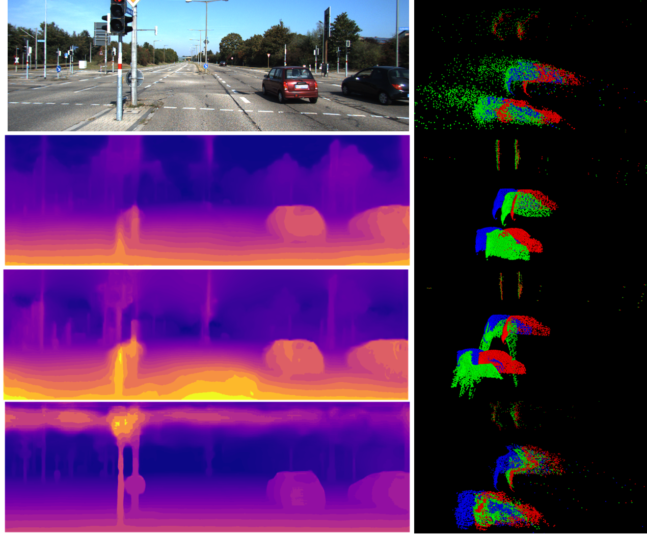
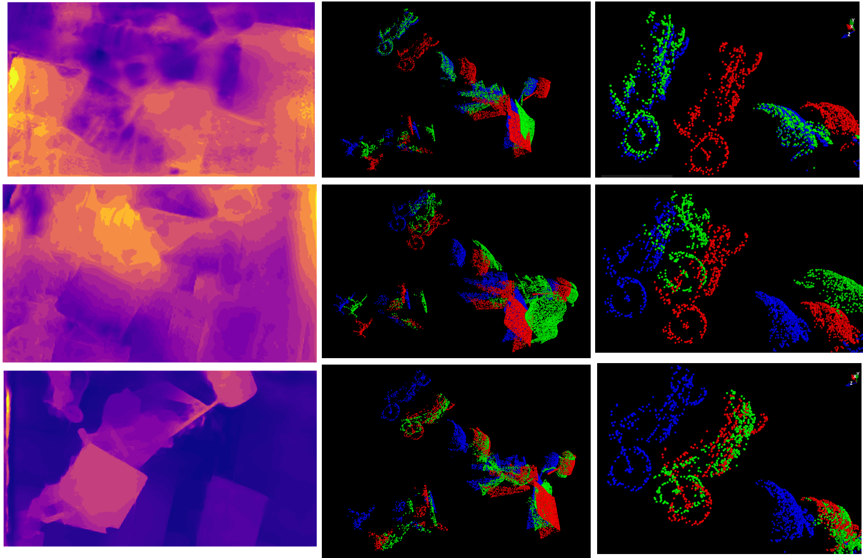
Figure 5: Qualitative depth and real-scale 3D scene flow results of the proposed MonoPLFlowNet on KITTI and Flyingthins3D for a single pair of two consecutive frames. For KITTI (column 1&2), 1st row: 1st frame of the RGB input image, recovered scene flow of [48] by our depth. From 2nd to 4th row: depth and scene flow by Mono-sf[18], Mono-sf-multi[19] and ours. For Flyingthings3D (column3&4&5), from top to down: depth of the 1st frame, scene flow, zoom-in view scene flow by [18, 19] and ours, original input RGB is shown in supplementary materials. Depth and scene flow of [18, 19] are recovered to the real scale before generating point cloud.

Most image-based scene flow works are trained on KITTI in a self-supervised manner, which leads to the scale ambiguity. We train our scene flow decoder in a fully-supervised manner with the EPE3D and forward-backward loss proposed in Section 3.4, which is able to estimate real-scale depth and scene flow. While real dataset like KITTI lacks 3D scene flow label, we only train our depth decoder on synthetic dataset Flyingthings3D.

Previous image-based scene flow works mostly use $d1,d2,f1,sf1$ for evaluation, but these metrics are designed for evaluating 2D optical flow or normalized scene flow, which themselves have the scale ambiguity. Instead, we use the metrics directly for evaluating real-scale 3D scene flow [27, 15, 46], which we refer as LiDAR-based evaluation standard (details in supplementary materials). However, since this LiDAR standard is too strict to image-based approaches, we slightly relax the LiDAR standard and use an image-based evaluation standard, EPE (end point error) 3D/2D are same to LiDAR standard:

• Acc3DS: the percentage of points with EPE3D $<$ 0.3m or relative error $<$ 0.1.

• Acc3DR: the percentage of points with EPE3D $<$ 0.4m or relative error $<$ 0.2.

• Outliers3D: the percentage of points with EPE3D $>$ 0.5m or relative error $>$ 0.3.

• Acc2D: the percentage of points whose EPE2D $<$ 20px or relative error $<$ 0.2.

Since we are the only monocular image-based approach estimating in real scale, to evaluate other works with our monocular approach, we need to recover other works to the real scale using the depth and scene flow ground truth (details in supplementary materials).

Flyingthings3D: Table 4 shows the monocular 3D scene flow comparison on Flyingthings3D. Even recovering [18, 19] to real scale with ground truth, our result still outperforms the two strongest state-of-the-art baseline works by an overwhelming advantage, more important we only need two consecutive images without any ground truth.

KITTI: We also directly evaluate scene flow on KITTI without any fine-tuning as shown in Table 4. The table also includes state-of-the-art 2D approach Mono-Expansion[48]. We first recover its direct output 2D optical flow to 3D scene flow, and then recover the scale. To recover 2D to 3D, Mono-Expansion proposed a strategy using LiDAR ground truth to expand 2D to 3D specifically for its own usage, but it is not able to extend to all works. For comparison, we recover 3D flow and scale in the same way with ground truth. In the table, the proposed approach still outperforms all state-of-the-art strong baseline works without any fine-tuning on KITTI. Since Mono-Expansion does not estimate depth, we use our depth and Mono-SF depth to help recovering 3D scene flow. Note that our scene flow decoder does not use the depth directly, but share the features and regress in parallel. In the table, by using our depth to recover Mono-Exp, it greatly outperforms by using depth from Mono-SF [18]. This comparison also shows the superiority of our depth estimation over others.

Ablation Study: We perform the ablation study for our scene flow decoder. The ablation study verifies the 2D-3D features alignment process, discussed in Section 3.3. As our MonoPLFlowNet architecture (Figure 2) shows, we perform three-level 2D-3D features alignment in our full model and decode in parallel, which are level 1, 2, 4. In the ablation study, we train the model only with level1 and level1+level2, and compare to the full model trained to the same epoch. The results indicate that the performances get better with deeper levels involved, hence the concatenation of features from different levels in the lattice boost the training, which proves our 2D-3D features alignment mechanism.

4.3 Visual Results

We show our visual results of depth and real-scale scene flow in Figure 5. 3D scene flow are visualized with the pseudo point cloud generating from the estimated depth map, where blue points are from 1st frame, red and green points are blue points translated to 2nd frame by ground truth and estimated 3D scene flow, respectively. The goal of the algorithm is to match the green points to the red points. Different to LiDAR-based works that have same shape of point cloud, the shapes of point cloud are different here because generating from different depth estimation. More visual results are in supplementary materials.

5 Conclusion

We present MonoPLFlowNet in this paper. It is the first deep learning architecture that can estimate both depth and 3D scene flow in real scale, using only two consecutive monocular images. Our depth and 3D scene flow estimation outperforms all the-state-of-art baseline monocular based works, and is comparable to LiDAR based works. In the future, we will explore the usage of more real datasets with specifically designed self-supervised loss to further improve the performance.

References

- [1] Andrew Adams, Jongmin Baek, and Myers Abraham Davis. Fast high‐dimensional filtering using the permutohedral lattice. Computer Graphics Forum, 29, 2010.
- [2] Aseem Behl, Omid Hosseini Jafari, Siva Karthik Mustikovela, Hassan Abu Alhaija, Carsten Rother, and Andreas Geiger. Bounding boxes, segmentations and object coordinates: How important is recognition for 3d scene flow estimation in autonomous driving scenarios? In 2017 IEEE International Conference on Computer Vision (ICCV), pages 2593–2602, 2017.
- [3] Aseem Behl, Despoina Paschalidou, Simon Donné, and Andreas Geiger. Pointflownet: Learning representations for rigid motion estimation from point clouds. In 2019 IEEE/CVF Conference on Computer Vision and Pattern Recognition (CVPR), pages 7954–7963, 2019.
- [4] P.J. Besl and Neil D. McKay. A method for registration of 3-d shapes. IEEE Transactions on Pattern Analysis and Machine Intelligence, 14(2):239–256, 1992.
- [5] Thomas Brox and Jitendra Malik. Large displacement optical flow: Descriptor matching in variational motion estimation. IEEE Transactions on Pattern Analysis and Machine Intelligence, 33(3):500–513, 2011.
- [6] R. Qi Charles, Hao Su, Mo Kaichun, and Leonidas J. Guibas. Pointnet: Deep learning on point sets for 3d classification and segmentation. In 2017 IEEE Conference on Computer Vision and Pattern Recognition (CVPR), pages 77–85, 2017.
- [7] Liang-Chieh Chen, George Papandreou, Iasonas Kokkinos, Kevin Murphy, and Alan L. Yuille. Deeplab: Semantic image segmentation with deep convolutional nets, atrous convolution, and fully connected crfs. IEEE Transactions on Pattern Analysis and Machine Intelligence, 40(4):834–848, 2018.
- [8] Yuhua Chen, Cordelia Schmid, and Cristian Sminchisescu. Self-supervised learning with geometric constraints in monocular video: Connecting flow, depth, and camera. In 2019 IEEE/CVF International Conference on Computer Vision (ICCV), pages 7062–7071, 2019.
- [9] Alexey Dosovitskiy, Philipp Fischer, Eddy Ilg, Philip Häusser, Caner Hazirbas, Vladimir Golkov, Patrick van der Smagt, Daniel Cremers, and Thomas Brox. Flownet: Learning optical flow with convolutional networks. In 2015 IEEE International Conference on Computer Vision (ICCV), pages 2758–2766, 2015.
- [10] David Eigen, Christian Puhrsch, and Rob Fergus. Depth map prediction from a single image using a multi-scale deep network. In Z. Ghahramani, M. Welling, C. Cortes, N. Lawrence, and K. Q. Weinberger, editors, Advances in Neural Information Processing Systems, volume 27. Curran Associates, Inc., 2014.
- [11] Huan Fu, Mingming Gong, Chaohui Wang, Kayhan Batmanghelich, and Dacheng Tao. Deep ordinal regression network for monocular depth estimation. In 2018 IEEE/CVF Conference on Computer Vision and Pattern Recognition, pages 2002–2011, 2018.
- [12] Yukang Gan, Xiangyu Xu, Wenxiu Sun, and Liang Lin. Monocular depth estimation with affinity, vertical pooling, and label enhancement. In Proceedings of the European Conference on Computer Vision (ECCV), September 2018.
- [13] Andreas Geiger, Philip Lenz, and Raquel Urtasun. Are we ready for autonomous driving? the kitti vision benchmark suite. In Conference on Computer Vision and Pattern Recognition (CVPR), 2012.
- [14] Clément Godard, Oisin Mac Aodha, and Gabriel J. Brostow. Unsupervised monocular depth estimation with left-right consistency. In 2017 IEEE Conference on Computer Vision and Pattern Recognition (CVPR), pages 6602–6611, 2017.
- [15] Xiuye Gu, Yijie Wang, Chongruo Wu, Yong Jae Lee, and Panqu Wang. Hplflownet: Hierarchical permutohedral lattice flownet for scene flow estimation on large-scale point clouds. In 2019 IEEE/CVF Conference on Computer Vision and Pattern Recognition (CVPR), pages 3249–3258, 2019.
- [16] Michael Hornácek, Andrew Fitzgibbon, and Carsten Rother. Sphereflow: 6 dof scene flow from rgb-d pairs. In 2014 IEEE Conference on Computer Vision and Pattern Recognition, pages 3526–3533, 2014.
- [17] Gao Huang, Zhuang Liu, Laurens Van Der Maaten, and Kilian Q. Weinberger. Densely connected convolutional networks. In 2017 IEEE Conference on Computer Vision and Pattern Recognition (CVPR), pages 2261–2269, 2017.
- [18] Junhwa Hur and Stefan Roth. Self-supervised monocular scene flow estimation. In 2020 IEEE/CVF Conference on Computer Vision and Pattern Recognition (CVPR), pages 7394–7403, 2020.
- [19] Junhwa Hur and Stefan Roth. Self-supervised multi-frame monocular scene flow. In Proceedings of the IEEE/CVF Conference on Computer Vision and Pattern Recognition (CVPR), pages 2684–2694, June 2021.
- [20] Mariano Jaimez, Mohamed Souiai, Jörg Stückler, Javier Gonzalez-Jimenez, and Daniel Cremers. Motion cooperation: Smooth piece-wise rigid scene flow from rgb-d images. In 2015 International Conference on 3D Vision, pages 64–72, 2015.
- [21] Varun Jampani, Martin Kiefel, and Peter V. Gehler. Learning sparse high dimensional filters: Image filtering, dense crfs and bilateral neural networks. In 2016 IEEE Conference on Computer Vision and Pattern Recognition (CVPR), pages 4452–4461, 2016.
- [22] Huaizu Jiang, Deqing Sun, Varun Jampani, Zhaoyang Lv, Erik Learned-Miller, and Jan Kautz. Sense: A shared encoder network for scene-flow estimation. In 2019 IEEE/CVF International Conference on Computer Vision (ICCV), pages 3194–3203, 2019.
- [23] Yevhen Kuznietsov, Jörg Stückler, and Bastian Leibe. Semi-supervised deep learning for monocular depth map prediction. In 2017 IEEE Conference on Computer Vision and Pattern Recognition (CVPR), pages 2215–2223, 2017.
- [24] Jin Han Lee, Myung-Kyu Han, Dong Wook Ko, and Il Hong Suh. From big to small: Multi-scale local planar guidance for monocular depth estimation. arXiv preprint arXiv:1907.10326, 2019.
- [25] Runfa Li and Truong Nguyen. Sm3d: Simultaneous monocular mapping and 3d detection. In 2021 IEEE International Conference on Image Processing (ICIP), pages 3652–3656, 2021.
- [26] Fayao Liu, Chunhua Shen, Guosheng Lin, and Ian Reid. Learning depth from single monocular images using deep convolutional neural fields. IEEE Transactions on Pattern Analysis and Machine Intelligence, 38(10):2024–2039, 2016.
- [27] Xingyu Liu, Charles R. Qi, and Leonidas J. Guibas. Flownet3d: Learning scene flow in 3d point clouds. In 2019 IEEE/CVF Conference on Computer Vision and Pattern Recognition (CVPR), pages 529–537, 2019.
- [28] Chenxu Luo, Zhenheng Yang, Peng Wang, Yang Wang, Wei Xu, Ram Nevatia, and Alan Yuille. Every pixel counts ++: Joint learning of geometry and motion with 3d holistic understanding. IEEE Transactions on Pattern Analysis and Machine Intelligence, 42(10):2624–2641, 2020.
- [29] Zhaoyang Lv, Kihwan Kim, Alejandro Troccoli, Deqing Sun, James Rehg, and Jan Kautz. Learning rigidity in dynamic scenes with a moving camera for 3d motion field estimation. In ECCV, 2018.
- [30] Wei-Chiu Ma, Shenlong Wang, Rui Hu, Yuwen Xiong, and Raquel Urtasun. Deep rigid instance scene flow. In 2019 IEEE/CVF Conference on Computer Vision and Pattern Recognition (CVPR), pages 3609–3617, 2019.
- [31] Nikolaus Mayer, Eddy Ilg, Philip Häusser, Philipp Fischer, Daniel Cremers, Alexey Dosovitskiy, and Thomas Brox. A large dataset to train convolutional networks for disparity, optical flow, and scene flow estimation. In 2016 IEEE Conference on Computer Vision and Pattern Recognition (CVPR), pages 4040–4048, 2016.
- [32] Moritz Menze and Andreas Geiger. Object scene flow for autonomous vehicles. In 2015 IEEE Conference on Computer Vision and Pattern Recognition (CVPR), pages 3061–3070, 2015.
- [33] Moritz Menze and Andreas Geiger. Object scene flow for autonomous vehicles. In 2015 IEEE Conference on Computer Vision and Pattern Recognition (CVPR), pages 3061–3070, 2015.
- [34] Himangi Mittal, Brian Okorn, and David Held. Just go with the flow: Self-supervised scene flow estimation. In 2020 IEEE/CVF Conference on Computer Vision and Pattern Recognition (CVPR), pages 11174–11182, 2020.
- [35] Andriy Myronenko and Xubo Song. Point set registration: Coherent point drift. IEEE Transactions on Pattern Analysis and Machine Intelligence, 32(12):2262–2275, 2010.
- [36] Charles R Qi, Li Yi, Hao Su, and Leonidas J Guibas. Pointnet++: Deep hierarchical feature learning on point sets in a metric space. NIPS, 2017.
- [37] Anurag Ranjan, Varun Jampani, Lukas Balles, Kihwan Kim, Deqing Sun, Jonas Wulff, and Michael J. Black. Competitive collaboration: Joint unsupervised learning of depth, camera motion, optical flow and motion segmentation. In 2019 IEEE/CVF Conference on Computer Vision and Pattern Recognition (CVPR), pages 12232–12241, 2019.
- [38] Ashutosh Saxena, Min Sun, and Andrew Y. Ng. Make3d: Learning 3d scene structure from a single still image. IEEE Transactions on Pattern Analysis and Machine Intelligence, 31(5):824–840, 2009.
- [39] Rene Schuster, Oliver Wasenmuller, Georg Kuschk, Christian Bailer, and Didier Stricker. Sceneflowfields: Dense interpolation of sparse scene flow correspondences. In 2018 IEEE Winter Conference on Applications of Computer Vision (WACV), pages 1056–1065, 2018.
- [40] Hang Su, Varun Jampani, Deqing Sun, Subhransu Maji, Evangelos Kalogerakis, Ming-Hsuan Yang, and Jan Kautz. Splatnet: Sparse lattice networks for point cloud processing. In 2018 IEEE/CVF Conference on Computer Vision and Pattern Recognition, pages 2530–2539, 2018.
- [41] Deqing Sun, Xiaodong Yang, Ming-Yu Liu, and Jan Kautz. Pwc-net: Cnns for optical flow using pyramid, warping, and cost volume. In 2018 IEEE/CVF Conference on Computer Vision and Pattern Recognition, pages 8934–8943, 2018.
- [42] Tatsunori Taniai, Sudipta N. Sinha, and Yoichi Sato. Fast multi-frame stereo scene flow with motion segmentation. In 2017 IEEE Conference on Computer Vision and Pattern Recognition (CVPR), pages 6891–6900, 2017.
- [43] Christoph Vogel, Konrad Schindler, and Stefan Roth. 3D scene flow estimation with a piecewise rigid scene model. International Journal of Computer Vision, 115(1):1–28, Oct. 2015.
- [44] Zirui Wang, Shuda Li, Henry Howard-Jenkins, Victor Adrian Prisacariu, and Min Chen. Flownet3d++: Geometric losses for deep scene flow estimation. In 2020 IEEE Winter Conference on Applications of Computer Vision (WACV), pages 91–98, 2020.
- [45] Anne S. Wannenwetsch, Martin Kiefel, Peter V. Gehler, and Stefan Roth. Learning task-specific generalized convolutions in the permutohedral lattice. In Pattern Recognition - 41st DAGM German Conference, DAGM GCPR 2019, Dortmund, Germany, September 10-13, 2019, Proceedings, volume 11824 of Lecture Notes in Computer Science, pages 345–359. Springer, 2019.
- [46] Wenxuan Wu, Zhi Yuan Wang, Zhuwen Li, Wei Liu, and Li Fuxin. Pointpwc-net: Cost volume on point clouds for (self-) supervised scene flow estimation. In European Conference on Computer Vision, pages 88–107. Springer, 2020.
- [47] Yufan Xu, Yan Wang, and Lei Guo. Unsupervised ego-motion and dense depth estimation with monocular video. In 2018 IEEE 18th International Conference on Communication Technology (ICCT), pages 1306–1310, 2018.
- [48] Gengshan Yang and Deva Ramanan. Upgrading optical flow to 3d scene flow through optical expansion. In 2020 IEEE/CVF Conference on Computer Vision and Pattern Recognition (CVPR), pages 1331–1340, 2020.
- [49] Maoke Yang, Kun Yu, Chi Zhang, Zhiwei Li, and Kuiyuan Yang. Denseaspp for semantic segmentation in street scenes. In 2018 IEEE/CVF Conference on Computer Vision and Pattern Recognition, pages 3684–3692, 2018.
- [50] Zhenheng Yang, Peng Wang, Yang Wang, Wei Xu, and Ram Nevatia. Every pixel counts: Unsupervised geometry learning with holistic 3d motion understanding, 2018.
- [51] Wei Yin, Yifan Liu, Chunhua Shen, and Youliang Yan. Enforcing geometric constraints of virtual normal for depth prediction. In 2019 IEEE/CVF International Conference on Computer Vision (ICCV), pages 5683–5692, 2019.
- [52] Zhichao Yin and Jianping Shi. Geonet: Unsupervised learning of dense depth, optical flow and camera pose. In 2018 IEEE/CVF Conference on Computer Vision and Pattern Recognition, pages 1983–1992, 2018.
- [53] Qian-Yi Zhou, Jaesik Park, and Vladlen Koltun. Fast global registration. In Bastian Leibe, Jiri Matas, Nicu Sebe, and Max Welling, editors, Computer Vision – ECCV 2016, pages 766–782, Cham, 2016. Springer International Publishing.
- [54] Yuliang Zou, Zelun Luo, and Jia-Bin Huang. Df-net: Unsupervised joint learning of depth and flow using cross-task consistency. In European Conference on Computer Vision, 2018.