Diffusiophoresis in a Near-critical Binary Fluid Mixture

Abstract

We consider placing a rigid spherical particle into a binary fluid mixture in the homogeneous phase near the demixing critical point. The particle surface is assumed to have a short-range interaction with each mixture component and to attract one component more than the other. Owing to large osmotic susceptibility, the adsorption layer, where the preferred component is more concentrated, can be of significant thickness. This causes a particle motion under an imposed composition gradient. Thus, diffusiophoresis emerges from a mechanism which has not been considered so far. We calculate how the mobility depends on the temperature and particle size.

Diffusiophoresis derja ; andersJFM ; SepPurMeth ; prieve ; anders ; staff has recently attracted much attention mainly because of their applications in lab-on-a-chip processes shin ; marb ; keh ; abecas ; volpe ; veleg ; osmflow ; kar ; shinPNAS ; frenkel ; vinze . They are conventionally discussed in terms of a solution in contact with a solid. A solution in the interfacial layer, generated immediately near a solid surface, can have distinct properties due to some interaction potential between a solute and a surface. When a gradient of solute concentration is imposed in the direction tangential to the surface, some force exerted on only the solution in the interfacial layer can yield the slip velocity between the solid and the bulk of the solution. Diffusiophoresis occurs when a solution has no convection far from a mobile surface, whereas diffusioosmosis occurs when a surface is fixed. If the solution is an electrolyte, the interfacial layer is the electric double layer. Otherwise, the layer can be generated by the van der Waals interaction or some dipole-dipole interaction.

Below, a binary fluid mixture, containing no ions, in the homogeneous phase close to the demixing critical point is considered and is simply referred to as a mixture. We can apply hydrodynamics for flow with a typical length sufficiently large in comparison to the correlation length of composition fluctuations, which are significant only on smaller length scales okafujiko ; furu . Suppose that a rigid spherical particle is placed into a mixture with the critical composition. A short-range interaction is assumed between each mixture component and the particle surface. The surface usually attracts one component more than the other Cahn ; binder ; holyst ; beyslieb ; beysest ; diehl97 , although this is not always the case beys2019 ; fujitani2021 . The adsorption layer, where the preferred component is more concentrated, can be of significant thickness because of large osmotic susceptibility. Assuming a mixture to be quiescent far from the particle, we previously calculated how the preferential adsorption (PA) affects the drag coefficient $\gamma_{\rm d}$, which is defined as the negative of the ratio of the drag force to a given particle velocity in the linear regime yabufuji .

We write $T$ for the temperature, $T_{\rm cr}$ for the critical temperature, and $\tau$ for the reduced temperature $|T-T_{\rm cr}|/T_{\rm cr}$. In the renormalized local functional theory fisher-auyang ; OkamotoOnuki , the free-energy functional (FEF) is coarse-grained up to the local correlation length, $\xi$. After coarse-grained, the composition’s equilibrium profile minimizes the FEF because many profiles that differ only on smaller length scales are unified into much fewer profiles OkamotoOnuki ; Yabu-On . In our previous work yabufuji , the hydrodynamics formulated from the coarse-grained FEF yabuokaon ; undul is used, and the critical composition is assumed far from the particle. There, $\xi$ becomes equal to $\xi_{0}\tau^{-\nu}$, which is denoted by $\xi_{\infty}$. Here, $\xi_{0}$ is a non-universal length of molecular size and $\nu\ (\approx 0.630)$ is a critical exponent peli . We assume $\xi\gg\xi_{0}$. The PA significantly affects $\gamma_{\rm d}$ if the particle radius, $r_{0}$, is not much larger than $\xi_{\infty}$, which can indicate the thickness of the adsorption layer yabufuji . Even then, $\xi$ can be sufficiently small anywhere as compared with a typical length of the flow because of $\xi<\xi_{\infty}$ in the adsorption layer. Experimentally, $\xi_{\infty}$ can reach $100\$nm.

In this Letter, we use the hydrodynamics mentioned above to discuss diffusiophoresis caused by the PA onto the particle surface. As shown in Fig. 1, a neutrally buoyant particle lies in a mixture filled in a channel, which has dimensions much larger than $r_{0}$ and extends along the $z$ axis. We impose a composition difference between the reservoirs to create a weak composition gradient in the channel. The particle undergoes a stationary and translational motion free from the drag force. If the PA were also assumed onto the channel wall, the composition gradient would convect the mixture via diffusioosmosis wolynes ; pipe . In Fig. 1(b), we take a mixture region including the particle. Far from the particle in this region, which has dimensions much larger than $\xi_{\infty}$, the composition gradient becomes a constant vector and convection vanishes. In the following paragraphs, we will formulate this situation and calculate mobility, which represents the ratio of the particle velocity to the constant vector. An anisotropic stress in the adsorption layer causes diffusiopheresis and arises from the free energy in the bulk of a mixture, which does not involve any potential due to the surface because the length range each component interacts with the surface is invisible in our coarse-grained description. This mechanism is not considered in the conventional theory. In our problem, larger osmotic susceptibility should tend to increase the magnitude of mobility by thickening the adsorption layer, and have the opposite tendency by weakening the chemical-potential gradient under a given composition gradient. As a result, it is expected that the change in mobility with the reduced temperature $\tau$ can be nonmonotonic. The change with the particle radius $r_{0}$ is expected to be explicit unless $\xi_{\infty}/r_{0}$ is much smaller than unity. Our results are later shown to be consistent with the expectations. These properties may be utilized in manipulating colloidal particles.

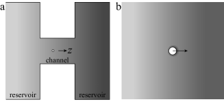
Figure 1: Schematic of the situation supposed in our formulation. The grayscale indicates the composition; a component is more concentrated in a darker region. (a) A mixture is filled in a container, where a channel connects two reservoirs. A particle, represented by a circle, passes through the channel, which extends along the $z$ axis. (b) A magnified view of a region including the particle. A darker region immediately near the particle represents the adsorption layer. The particle motion is represented by an arrow.

Naming the mixture components a and b, we write $\rho_{n}$ for the mass density of the component $n\ (=$ a or b$)$, and $\mu_{n}$ for the chemical potential conjugate to $\rho_{n}$. We write $\rho$ for $\rho_{\rm a}+\rho_{\rm b}$, $\varphi$ for $\rho_{\rm a}-\rho_{\rm b}$, and $\varphi_{\rm c}$ for the value of $\varphi$ at the critical composition. Hereafter, a quantity at the critical composition is generally indicated by the subscript _c. The order parameter is given by $\psi\equiv\varphi-\varphi_{\rm c}$. The chemical potential conjugate to $\varphi$ is given by $(\mu_{\rm a}-\mu_{\rm b})/2$, and its deviation from the value at the critical point is denoted by $\mu$, which is simply called the chemical potential here. We write $c_{n}$ for the mass fraction of the component $n$; $c_{n}=\rho_{n}/\rho$ and $\varphi=\rho(2c_{\rm a}-1)$ hold. We use the conventional symbols for the critical exponents, $\beta,\ \gamma$, and $\eta$, and have $\eta{\approx 0.0364}$ (peli, ). The (hyper)scaling relations give $2\beta+\gamma=3\nu$ and $\gamma=\nu(2-\eta)$.

The coarse-grained FEF is separated into the $\rho$-dependent part and $\psi$-dependent part. The latter part in the bulk of a mixture, denoted by ${\cal F}_{\rm b}[\psi]$, is given by the volume integral of

$$f_{\rm b}(\psi)+\frac{1}{2}K(\psi)\left|\nabla\psi\right|^{2}-\mu\varphi$$ (1)

over the mixture. Derived in Ref. OkamotoOnuki , $f_{\rm b}{(\geq 0)}$ and $K{(>0)}$ are even functions of $\psi$, as shown in the supplementary material. The corresponding integrand for the $\rho$-dependent part is independent of the derivatives of $\rho$. The difference in the components’ interactions with the surface contributes to the FEF and is described by the area integration of a function of $\varphi$ over the particle surface. Assuming it to be a linear function, we write $h$ for the negative of the coefficient of $\varphi$; $h$ is called the surface field. The sum of the area integration and ${\cal F}_{\rm b}[\psi]$ gives the $\psi$-dependent part, denoted by ${\cal F}[\psi]$. At equilibrium, $\mu$ is homogeneous. In general, $\mu$ can depend on the position $r$, $\psi$ minimizing ${\cal F}[\psi]$ gives the coarse-grained profile, and the minimum of ${\cal F}[\psi]$ gives a part of the grand potential.

The reversible part of the pressure tensor originating from ${\cal F}_{\rm b}$ is denoted by ${\mathsf{\Pi}}$. We can define $p$ so that $p{\mathsf{1}}$ is the one from the $\rho$-dependent part. Here, ${\mathsf{1}}$ denotes the second-order isotropic tensor whose components with respect to rectangular coordinates are represented by Kronecker’s delta, and $p$ is the scalar pressure in the absence of ${\cal F}$. The reversible part of the pressure tensor is thus given by $p{\mathsf{1}}+{\mathsf{\Pi}}$ in the bulk of a mixture. As in the model H Hohen-Halp , ${\mathsf{\Pi}}$ is obtained by subtracting the product of ${\mathsf{1}}$ and Eq. (1) from $K\nabla\psi\nabla\psi$ onukibook ; onukiPRE . If $\psi$ is homogeneous, the scalar pressure, denoted by $P$, equals $p-f_{\rm b}(\psi)+\mu\varphi$.

In the reference state, where a particle is at rest in an equilibrium mixture with the critical composition far from the particle, the chemical potential $\mu$ vanishes and the total mass density $\rho$ is homogeneous. A difference in the composition $c_{\rm a}$ between the reservoirs is imposed as a perturbation on this state. Assuming the difference to be proportional to a dimensionless smallness parameter $\varepsilon$, we consider the velocity of a force-free particle up to the order of $\varepsilon$. In a frame fixed to the container, we define $U$ so that the particle velocity equals $\varepsilon U{\mbox{\boldmath$e$}}_{z}$ up to the order of $\varepsilon$, where ${\mbox{\boldmath$e$}}_{z}$ is the unit vector along the $z$ axis. With $v$ denoting the velocity field of a mixture, the no-slip boundary condition gives ${\mbox{\boldmath$v$}}=\varepsilon U{\mbox{\boldmath$e$}}_{z}$ at the particle surface. Far from the particle in Fig. 1(b), because $\nabla P={\mbox{\boldmath$0$}}$ is assumed there and no PA is assumed onto the channel wall, interdiffusion occurs between the components under ${\mbox{\boldmath$v$}}={\mbox{\boldmath$0$}}$. The composition gradient there is proportional to $\nabla\mu$ multiplied by the osmotic susceptibility.

Up to the order of $\varepsilon$, because $\rho$ is stationary in the frame co-moving with the particle center, we can assume the incompressibility condition $\nabla\cdot{\mbox{\boldmath$v$}}=0$. In a frame fixed to the container, the time derivative of $\varphi$ is equal to the negative of the divergence of the sum of the convective flux, $\varphi{\mbox{\boldmath$v$}}$, and the diffusive flux. The latter is given by $-L(\psi)\nabla\mu$, where a function $L(\psi)$ represents the transport coefficient for the interdiffusion. We thus have $\left({\mbox{\boldmath$v$}}-\varepsilon U{\mbox{\boldmath$e$}}_{z}\right)\cdot\nabla\psi=\nabla\cdot\left[L(\psi)\nabla\mu\right]$ with the aid of the stationarity in the co-moving frame up to the order of $\varepsilon$. We consider a particular instant, when the particle center passes the origin of the polar coordinate system $(r,\theta,\phi)$ fixed to the container. The $z$ axis is taken as the polar axis. A mixture does not diffuse into the particle, which yields $\partial_{r}\mu=0$ at $r=r_{0}$. Here, $\partial_{r}$ indicates the partial derivative with respect to $r$.

Correlated clusters of the order parameter are convected on length scales smaller than $\xi$, which enhances $L$ kawasaki ; seng . The quotient of $L(0)$ divided by the osmotic susceptibility gives the diffusion coefficient for the relaxation of equilibrium order-parameter fluctuations at the critical composition. According to the mode-coupling theory kawasaki ; onukibook , the quotient equals the self-diffusion coefficient obtained by applying the Stokes law stokes and Sutherland-Einstein relation suther ; eins for a rigid sphere having a radius equal to $\xi$. We simply extend this result to a homogeneous off-critical composition, and use the extended result, $L(\psi)=k_{\rm B}T/[{6\pi\eta_{\rm s}\xi f_{\rm b}^{\prime\prime}(\psi)}]$, in the dynamics yabufuji . Here, $\xi$ and $\psi$ imply their respective local values and $k_{\rm B}$ denotes the Boltzmann constant. The shear viscosity, denoted by $\eta_{\rm s}$, is assumed to be constant, with its weak singularity neglected. The (double) prime represents the (second-order) derivative with respect to the variable. The osmotic susceptibility, with $T$ and $\rho$ kept constant, is given by $1/f_{\rm b}^{\prime\prime}(\psi)$, which is proportional to $\tau^{-\gamma}$ for $\psi=0$ in the critical regime. We use $\nabla\cdot{\mathsf{\Pi}}=\varphi\nabla\mu$ and the Stokes approximation to obtain $0=-\nabla p-\varphi\nabla\mu+\eta_{\rm s}\Delta{\mbox{\boldmath$v$}}$ from the law of momentum conservation.

A superscript ⁽⁰⁾ is added to a field in the reference state, where the order parameter can be written as $\psi^{(0)}(r)$ because of the symmetry. We define $p_{+}$ as $p+\varphi_{\rm c}\mu$. Up to the order of $\varepsilon$, we expand the fields as $\psi({\mbox{\boldmath$r$}})=\psi^{(0)}(r)+\varepsilon\psi^{(1)}({\mbox{\boldmath$r$}})$, ${p}_{+}({\mbox{\boldmath$r$}})={p}_{+}^{(0)}+\varepsilon{p}_{+}^{(1)}({\mbox{\boldmath$r$}})$, $\mu({\mbox{\boldmath$r$}})=\varepsilon\mu^{(1)}({\mbox{\boldmath$r$}})$, and ${\mbox{\boldmath$v$}}({\mbox{\boldmath$r$}})=\varepsilon{\mbox{\boldmath$v$}}^{(1)}({\mbox{\boldmath$r$}})$. A field with the superscript ⁽¹⁾ is defined so that it becomes at the order of $\varepsilon$ after being multiplied by $\varepsilon$. Far from the particle, $p_{+}^{(1)}$ becomes constant because there $\varepsilon p_{+}^{(1)}$ equals $P$ at the order of $\varepsilon$. Up to the order of $\varepsilon$, the interdiffusion is described by

$$\left({\mbox{\boldmath$v$}}^{(1)}-U{\mbox{\boldmath$e$}}_{z}\right)\cdot\nabla\psi^{(0)}=\nabla\cdot\left[L(\psi^{(0)})\nabla\mu^{(1)}\right]\ ,$$ (2)

which equals ${\psi^{(0)}}^{\prime}L^{\prime}\partial_{r}\mu^{(1)}+L\Delta\mu^{(1)}$, and the momentum conservation is described by

$$0=-\nabla p_{+}^{(1)}-\psi^{(0)}\nabla\mu^{(1)}+\eta_{\rm s}\Delta{\mbox{\boldmath$v$}}^{(1)}\ .$$ (3)

We define $\tau_{*}$ as $(\xi_{0}/{r_{0}})^{1/\nu}$ to use ${\hat{\tau}}\equiv\tau/\tau_{*}$, and define $L_{*}$ as $L(0)$ at $\tau=\tau_{*}$ to have $L(0)={\hat{\tau}}^{\nu\eta-\nu}L_{*}$. Because of the particle-motion symmetry, the angular dependence of $\mu^{(1)}$ and that of $v_{r}^{(1)}$ are only via $\cos{\theta}$, that of $v_{\theta}^{(1)}({\mbox{\boldmath$r$}})$ only via $\sin{\theta}$, and $v_{\phi}^{(1)}$ vanishes fpd . A spatially constant term in $\mu$, if any, does not affect our calculation and can be neglected. We nondimensionalize $\mu^{(1)}$ and $v_{r}^{(1)}$ to define functions ${\cal Q}$ and ${\cal R}$ so that

$${\cal Q}({\hat{r}})\cos{\theta}=\frac{\sqrt{L_{*}}\mu^{(1)}({\mbox{\boldmath$r$}})}{U\sqrt{5\eta_{\rm s}}}\quad{\rm and}\quad{\cal R}({\hat{r}})\cos{\theta}=\frac{v_{r}^{(1)}({\mbox{\boldmath$r$}})}{U}$$ (4)

hold, where ${\hat{r}}$ denotes the dimensionless radial distance $r/r_{0}$. Writing ${\cal D}_{m}$ for ${\hat{r}}\partial_{\hat{r}}+m$ and defining $\Phi({\hat{r}})$ as $-{r^{2}}{\psi^{(0)}}^{\prime}(r_{0}{\hat{r}})/[3\sqrt{5\eta_{\rm s}L_{*}}]$, we rewrite Eq. (2) as

$${\cal D}_{-1}{\cal D}_{2}{\cal Q}({\hat{r}})=-3\Phi({\hat{r}})\left[{\cal A}({\hat{r}})\left({\cal R}({\hat{r}})-1\right)-{\cal B}({\hat{r}}){\cal Q}^{\prime}({\hat{r}})\right]\ ,$$ (5)

whose left-hand side comes from $\Delta\mu^{(1)}$. In the supplementary material, definitions of ${\cal A}$ and ${\cal B}$ and some equilibrium order-parameter profiles are presented. From the incompressibility condition and the $r$ and $\theta$ components of Eq. (3), we eliminate $p_{+}^{(1)}$ and $v_{\theta}^{(1)}$ to obtain

$${\cal D}_{1}{\cal D}_{-2}{\cal D}_{3}{\cal D}_{0}{\cal R}({\hat{r}})=-30\Phi({\hat{r}}){\cal Q}({\hat{r}})\ .$$ (6)

These two equations are derived in Ref. yabufuji . The boundary conditions for ${\cal Q}$ and ${\cal R}$, respectively derived from those for $\mu$ and $v$, are the same as given in Ref. yabufuji except that ${\cal Q}({\hat{r}})$ is proportional to ${\hat{r}}$ far from the particle. We write ${g}$ for the constant of proportionality; Ref. yabufuji supposes ${g}=0$. Far from the particle, $\nabla\mu$, and thus $\nabla c_{\rm a}$, are proportional to $\varepsilon{\mbox{\boldmath$e$}}_{z}$ up to the order of $\varepsilon$.

Applying the boundary conditions, we can transform Eq. (5) so that ${\cal Q}$ equals the sum of the solution in the absence of the right-hand side (RHS) and the convolution of a kernel and the RHS. We can transform Eq. (6) similarly by using another kernel. The kernels are respectively denoted by $\Gamma_{\rm Q}$ and $\Gamma_{\rm R}$, which are obtained in Ref. okafujiko . As in Ref. yabufuji , we assume that the RHSs are multiplied by an artificial parameter $\kappa$. Accordingly, rewriting ${\cal Q}$ as ${\tilde{\cal Q}}_{\kappa}$ and ${\cal R}$ as ${\tilde{\cal R}}_{\kappa}$, we have simultaneous integral equations for ${\tilde{\cal Q}}_{\kappa}$ and ${\tilde{\cal R}}_{\kappa}$. They are shown in the supplementary material, together with the definitions of the kernels. We find ${\tilde{\cal Q}}_{0}({\hat{r}})$ equal to ${g}({\hat{r}}+({\hat{r}}^{-2}/2))$, which is below referred to as $q_{0}({\hat{r}})$. Eliminating ${\tilde{\cal R}}_{\kappa}$ from the integral equations, and expanding ${\tilde{\cal Q}}_{\kappa}$ with respect to $\kappa$ as ${\tilde{\cal Q}}_{\kappa}({\hat{r}})=\sum_{n=0}^{\infty}{q}_{n}({\hat{r}})\kappa^{n}$, we obtain a recurrence relation for the expansion coefficients, $q_{0},q_{1},q_{2},\ldots$, as

$${q}_{n}({\hat{r}})=\int_{1}^{\infty}d{\hat{s}}\ \Gamma_{\rm Q}\left({\hat{r}},{\hat{s}}\right)\Phi\left({\hat{s}}\right)\Big{[}-{\cal B}\left({\hat{s}}\right)q_{n-1}^{\prime}\left({\hat{s}}\right)$$

$$\quad+{\cal A}({\hat{s}})\int_{1}^{\infty}d{\hat{u}}\ \Gamma_{\rm R}\left({\hat{s}},{\hat{u}}\right)\Phi\left({\hat{u}}\right)q_{n-2}\left({\hat{u}}\right)\Big{]}$$ (7)

for $n=1,2,3,\ldots$. Here, for $n=1$, the integral with respect to ${\hat{u}}$ is replaced by $\alpha_{0}({\hat{s}})\equiv(3{\hat{s}}^{-1}/2)-({\hat{s}}^{-3}/2)-1$. The original solutions of ${\cal Q}$ and ${\cal R}$ are respectively given by ${\tilde{\cal Q}}_{1}$ and ${\tilde{\cal R}}_{1}$.

The drag coefficient for a value of $g$ in general deviates from the Stokes law, $6\pi\eta_{\rm s}r_{0}$, owing to the PA and the imposed gradient. For the drag coefficient considered here, Eq. (3.28) of Ref. yabufuji remains valid. Its derivation is outlined in the supplementary material. Thus, writing $\Delta{\hat{\gamma}}_{\rm d}$ for the ratio of the deviation to the Stokes law, we find $\Delta{\hat{\gamma}}_{\rm d}$ to be given by the integral of $10\alpha_{0}({\hat{r}})\Phi({\hat{r}}){\cal Q}({\hat{r}})/3$ from ${\hat{r}}=1$ to $\infty$. Obtaining $q_{n}$ from Eq. (7) and replacing ${\cal Q}$ by $q_{n}$ in the integral above, we find that the sum of the integrals over $n=0,1,2\ldots$ gives $\Delta{\hat{\gamma}}_{\rm d}$. Unless otherwise stated, we truncate this series suitably to calculate $\Delta{\hat{\gamma}}_{\rm d}$ numerically, with the aid of the software Mathematica (Wolfram Research). From the governing equations and the boundary conditions for ${\cal Q}$ and ${\cal R}$, we find $\Delta{\hat{\gamma}}_{\rm d}$ to be a linear function of ${g}$. The linear function, which is obtained by calculating $\Delta{\hat{\gamma}}_{\rm d}$ for ${g}=0$ and $1$, determines the value of ${g}$ making the drag force vanish, i.e., yielding $\Delta{\hat{\gamma}}_{\rm d}=-1$. This value is denoted by $g_{0}$. We note that $g$ is a dimensionless value of $\partial_{z}\mu^{(1)}$ far from the particle with the velocity $\varepsilon U{\mbox{\boldmath$e$}}_{z}$. The sign of $\psi^{(0)}$ is changed by changing that of the surface field $h$, and thus we find $g_{0}$ to be an odd function of $h$. In the absence of PA $(h=0)$, the second term on the RHS of Eq. (3) vanishes, $\Delta{\hat{\gamma}}_{\rm d}$ vanishes irrespective of $g$, $g_{0}$ cannot be obtained, and diffusiophoresis does not appear.

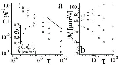
Figure 2: By setting the particle radius $r_{0}$ equal to $0.1\ \mu$m. we plot a dimensionless coefficient $1/g_{0}$ in (a) and the mobility ${\cal M}$ in (b) against the reduced temperature $\tau$. Linked via Eq. (8), they are proportional to the particle speeds under given gradients of the chemical potential $\mu$ and the composition $c_{\rm a}$ far from the particle, respectively. The results shown by the symbols $+$, $\triangle$, $\circ$, and $\square$ are respectively obtained by setting the surface field $h$, defined below Eq. (1), equal to $1.73\times 10^{-1},\ 3.46\times 10^{-2},\ 1.55\times 10^{-2}$, and $6.91\times 10^{-3}\$cm${}^{3}/$s². The reference line in (a) has the slope of $-\gamma$. In the inset, $1/g_{0}$ is plotted against $h$ for $\tau=4.05\times 10^{-4}$ and $r_{0}=0.1\ \mu$m. For its result on the extreme right, the series for the deviation ratio of the drag coefficient $\Delta{\hat{\gamma}}_{\rm d}$ numerically diverges and the Borel summation is applied instead of the suitable truncation.

We first assume the chemical-potential gradient $\nabla\mu{\ \left(\propto\varepsilon{\mbox{\boldmath$e$}}_{z}\right)}$ to be given far from the particle. The velocity of a force-free particle equals the product of the given gradient, $r_{0}\sqrt{L_{*}/5\eta_{\rm s}}$, and $1/g_{0}$, because of the first entry of Eq. (4). Below, we use the parameter values by supposing a mixture of 2,6-lutidine and water (LW), which has $T_{\rm cr}=307\$K, $c_{\rm ac}=0.290$, and $\xi_{0}=0.198\$nm mirz . In Fig. 2(a), we find for $h>0$ that $1/g_{0}$, being positive, increases as the reduced temperature $\tau$ decreases and as the surface field $h$ increases. This increase of $1/g_{0}$ is expected because then the PA is stronger. In the inset of Fig. 2(a), the increase of $1/g_{0}$ with $h$ becomes more gradual as $h$ increases for the value of $\tau$. In the supplementary material, we show some flow profiles, which are consistent with our coarse-grained description.

To consider the diffusiophoretic mobility, we then assume the composition gradient $\nabla c_{\rm a}\ \left(\propto\varepsilon{\mbox{\boldmath$e$}}_{z}\right)$ to be given far from the particle. Writing ${c_{\rm a}^{\prime}}_{\infty}$ for the $z$ component of the given gradient, we define the mobility ${\cal M}$ so that $\varepsilon U={\cal M}{c_{\rm a}^{\prime}}_{\infty}/c_{\rm ac}$ holds, and have

$${\cal M}=\frac{r_{0}c_{\rm ac}\sqrt{L_{*}}}{g_{0}\sqrt{5\eta_{\rm s}}}\times\left.\frac{\partial\mu}{\partial c_{\rm a}}\right)_{TP}\ .$$ (8)

Here, the partial derivative, with $(T,P)$ fixed, is evaluated far from the particle in the reference state. It is positive because of the thermodynamic stability. Thus, the particle moves toward the reservoir where the component preferred by the particle surface is more concentrated, as shown in Fig. 1(b). The conventional diffusiophoresis has a similar property anders ; staff . As shown in the supplementary material, the partial derivative approximately equals $2\rho_{\rm c}f_{\rm b}^{\prime\prime}(0)\ (\propto\tau^{\gamma})$. In Fig. 2(b), the slope of ${\cal M}$ is negative at $\tau\approx 10^{-2}$ for each value of $h$. Except for the smallest value of $h$, the slope is positive for small $\tau$ and the value of $\tau$ at the peak of ${\cal M}$ increases with $h$. The slope becomes negative when the decrease of $1/g_{0}$ with increasing $\tau$, shown in Fig. 2(a), overcomes the increase of $\tau^{\gamma}$. In Fig. 3, the mobility ${\cal M}$ increases with the particle radius $r_{0}$, as in the conventional theory anders ; mood . The increase is more noticeable when $r_{0}$ is smaller than approximately $0.2\ \mu$m at the larger value of $\tau$.

Suppose that the difference in $c_{\rm a}$ between the reservoirs is $c_{\rm ac}/10$ and that the channel length is $10\ \mu$m. The composition then remains close to the critical one over the channel. If we adopt ${\cal M}=50\ \mu$m${}^{2}/$s from Fig. 2(b), the particle speed is $0.5\ \mu$m$/$s for $r_{0}=0.1\ \mu$m. For Eq. (3) to be meaningful under $h\neq 0$, $\psi^{(0)}$ is required to be much larger than $\varepsilon\psi^{(1)}$ somewhere. Considering that the perturbation involves the velocity field, this requirement can be simplified in terms of a typical energy per unit area as $\eta_{\rm s}\left|\varepsilon U\right|\ll\left|h\psi^{(0)}(r_{0})\right|$. This is satisfied in the example presented here, as illustrated in the supplementary material. As $\tau$ increases well beyond the range of Fig. 2, $\xi_{\infty}$ approaches a molecular size and the anisotropic stress becomes ill-defined. Then, because of the background contribution to the osmotic susceptibility seng ; swinney , the partial derivative in Eq. (8) should stop increasing in proportion to $\tau^{\gamma}$. The mobility should then be explained in terms of the conventional mechanism rather than the PA.

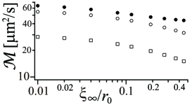
Figure 3: We plot the mobility ${\cal M}$ against a dimensionless correlation length far from the particle in the reference state $\xi_{\infty}/r_{0}$, which indicates a relative thickness of the adsorption layer. As mentioned in the supplementary material, $L_{*}$ in Eq. (8) depends on the particle radius $r_{0}$. Solid and open circles represent results for $\tau=1.82\times 10^{-4}$ and $7.14\times 10^{-4}$, respectively, under $h=1.55\times 10^{-2}\$cm${}^{3}/$s². For these values of $\tau$, $\xi_{\infty}$ equals $45.0$ and $19.0\$nm, respectively. Squares represent results for $\tau=7.14\times 10^{-4}$ and $h=6.91\times 10^{-3}\$cm${}^{3}/$s².

It is demonstrated in Ref. mood that, for nanocolloids in a nonelectrolyte solution, the diffusiophoretic mobility in the conventional theory can also be obtained by molecular dynamics simulation. We naively convert the second result from the right end in their Fig. 3(c) to ${\cal M}=1.6\times 10^{2}\ \mu$m${}^{2}/$s for a mixture of LW by taking 2,6-lutidine as the component a and by using $k_{\rm B}T_{\rm cr}$ and $\xi_{0}$ as the unit energy and length, respectively. The potential for the interaction between the nanocolloid and the solute is mentioned in Ref. mood . Regarding it as representing the adsorption of the component a and assuming the length of the interaction range to be the unit length, we tentatively convert its value at the surface of the immobile region to $h=1.0\$cm${}^{3}/$s². Noting that the converted values of ${\cal M}$ and $h$ are linked via the unit energy and neglecting the size dependence of the mobility, we can deduce that the values of ${\cal M}$ shown by the cross and square in Fig. 2(b) of the present study would approximately become $60$ and $10\ \mu$m${}^{2}/$s, respectively, in the range of $\tau$ validating the conventional theory. It is thus possible, for $h>0$, that the mobility for large $h$ is made smaller inside the critical regime than outside by larger osmotic susceptibility, and that the mobility for small $h$ is made larger inside the critical regime by thicker adsorption layer. This possibility clearly needs further investigation, particularly because the converted values are highly dependent on the unit length.

In this Letter, we theoretically show for diffusiophoresis in a nonelectrolyte fluid mixture near the demixing critical point that the mobility can have a large enough magnitude to be detected only in the critical regime, that its dependence on temperature can be changed qualitatively by the surface field, and that its dependence on particle radius can remain explicit even when the radius exceeds $0.1\ \mu$m.

Acknowledgements
The author thanks Dr. S. Yabunaka for stimulating discussion.

Supplemental Material
Here, we use the notation of the main text, and most of the contents in the first three paragraphs are described in more detail in Ref. yabufuji . In Ref. OkamotoOnuki , the coarse-grained FEF is derived from the Ginzburg-Landau-Wilson type of bare model and contains $\xi_{0}$, $C_{1}$ and $C_{2}$ as material constants. We obtain $C_{2}/(C_{1}\xi_{0})=2\pi^{2}/3$ from the renormalization-group calculation at the one loop order. We define $\omega$ as $(\xi_{0}/\xi)^{1/\nu}$, where $\xi$ is the local correlation length, and ${\hat{\omega}}$ as $\omega/\tau_{*}{\equiv(r_{0}/\xi)^{1/\nu}}$, where $r_{0}$ is the particle radius. A dimensionless order parameter ${\hat{\psi}}({\hat{r}})$ is defined as $\psi({r})/\psi_{*}$, where $\psi_{*}$ denotes $\tau_{*}^{\beta}/\sqrt{C_{2}}$ and the dimensionless radial distance ${\hat{r}}$ equals $r/r_{0}$. Introducing $\mu_{*}\equiv{k_{\rm B}{T}C_{1}\xi_{0}/(C_{2}r_{0}^{3}\psi_{*})}$, we define dimensionless chemical potential and surface field as ${\hat{\mu}}\equiv\mu/\mu_{*}$ and ${\hat{h}}\equiv h/\left(\mu_{*}r_{0}\right)$, respectively. We have $K(\psi){=}k_{\rm B}TC_{1}\omega^{-\eta\nu}$, and $f_{\rm b}(\psi){=}\mu_{*}\psi_{*}{\hat{f}}_{\rm b}(\psi/\psi_{*})$ with ${\hat{f}}_{\rm b}$ being defined as

$${\hat{f}}_{\rm b}({\hat{\psi}})={\hat{\omega}}^{\gamma-1}{\hat{\tau}}\left(\frac{{\hat{\psi}}^{2}}{2}+\frac{{\hat{\psi}}^{4}}{12{\hat{\omega}}^{2\beta-1}{\hat{\tau}}}\right)\ .$$ (9)

Hereafter, ${\hat{\omega}}$ is regarded as a function of ${\hat{\psi}}$ because of a self-consistent condition, ${\hat{\omega}}={\hat{\tau}}+{\hat{\omega}}^{1-2\beta}{\hat{\psi}}^{2}$. We have $\omega=\tau$ for $\psi=0$, and have $\xi=r_{0}$ for $\psi=\psi_{*}$ at $\tau=0$.

The order parameter in the reference state $\psi^{(0)}$, vanishing far from the particle, equals $\psi$ minimizing ${\cal F}[\psi]$ under $\mu=0$. The stationary condition yields

$${\hat{f}}_{\rm b}^{\prime}=-\frac{\eta\nu}{2}\frac{{\hat{\omega}}^{\prime}}{{\hat{\omega}}^{\eta\nu+1}}\left(\partial_{\hat{r}}{\hat{\psi}}\right)^{2}+\frac{1}{{\hat{\omega}}^{\eta\nu}}\left(\partial_{\hat{r}}^{2}+\frac{2}{{\hat{r}}}\partial_{\hat{r}}\right){\hat{\psi}}$$ (10)

for ${\hat{r}}>1$, together with $\partial_{\hat{r}}{\hat{\psi}}=-{\hat{h}}{\hat{\omega}}^{\eta\nu}$ at ${\hat{r}}=1$. Thus, ${\hat{\psi}}^{(0)}$ is totally determined by ${\hat{\tau}}$ and ${\hat{h}}$. The definition of $\Phi$ leads to $\Phi({\hat{r}})=-{\hat{r}}^{2}\partial_{\hat{r}}{\hat{\psi}}^{(0)}({\hat{r}})/{\sqrt{5\pi}}$; ${\cal A}({\hat{r}})$ and ${\cal B}({\hat{r}})$ are respectively given by $L_{*}/L(\psi^{(0)}(r_{0}{\hat{r}}))={\hat{f}}_{\rm b}^{\prime\prime}/{\hat{\omega}}^{\nu}$ and

$$\sqrt{5\eta_{\rm s}L_{*}}\frac{L^{\prime}(\psi^{(0)}(r_{0}{\hat{r}}))}{r_{0}L(\psi^{(0)}(r_{0}{\hat{r}}))}=\sqrt{{\frac{5\pi}{9}}}\left(\nu\frac{{\hat{\omega}}^{\prime}}{{\hat{\omega}}}-\frac{{\hat{f}}_{\rm b}^{\prime\prime\prime}}{{\hat{f}}_{\rm b}^{\prime\prime}}\right)\ .$$ (11)

No diffusive flux at the particle surface gives ${\cal Q}^{\prime}{(1)}=0$. We obtain $v_{\theta}^{(1)}/U=-\sin{\theta}[\partial_{\hat{r}}{\hat{r}}^{2}{\cal R}({\hat{r}})]/(2{\hat{r}})$ using the incompressibility condition. The no-slip boundary condition at the surface gives ${\cal R}{(1)}=1$ and ${\cal R}^{\prime}{(1)}=0$. Far from the particle, ${\cal R}$ vanishes and ${\cal Q}({\hat{r}})$ becomes $g{\hat{r}}$, which is consistent with Eqs. (5) and (6) because $\Phi$ vanishes there. Notably, $q_{0}$ satisfies the boundary conditions for ${\cal Q}$ and deletes the left-hand side (LHS) of Eq. (5).

In the main text, we modify Eqs. (5) and (6) by introducing $\kappa$. Defining ${\cal I}$ and ${\cal J}$ so that the modified RHSs respectively equal $\kappa{\cal I}({\hat{r}})$ and $\kappa{\cal J}({\hat{r}})$, we obtain

$${\tilde{\cal Q}}_{\kappa}\left({\hat{r}}\right)=q_{0}({\hat{r}})-\frac{\kappa}{3}\int_{1}^{\infty}d{\hat{s}}\ \varGamma_{{\rm Q}}\left({\hat{r}},{\hat{s}}\right){\cal I}({\hat{s}})\ ,$$ (12)

where $\varGamma_{\rm Q}(r,s)$ is given by $(r^{-2}s^{-2}/2)+r^{-2}s$ for $r\geq s$ and equals $\varGamma_{\rm Q}(s,r)$, and

$${\tilde{\cal R}}_{\kappa}\left({\hat{r}}\right)=1+\alpha_{0}({\hat{r}})-\frac{\kappa}{30}\int_{1}^{\infty}d{\hat{s}}\ \varGamma_{{\rm R}}\left({\hat{r}},{\hat{s}}\right){\cal J}({\hat{s}})\ .$$ (13)

Here, $\varGamma_{\rm R}(r,s)$ is given by the sum of $r^{-3}s^{2}-5r^{-1}$ and $(15r^{2}s^{2}-5r^{2}-5s^{2}+3)/(2r^{3}s^{3})$ for $r\geq s$, and equals $\varGamma_{\rm R}\left(s,r\right)$. Equations (12) and (13) are the integral equations mentioned above Eq. (7). With ${\mathsf{E}}$ denoting the rate-of-strain tensor, the drag force is given by the area integral of the dot product of $-p{\mathsf{1}}-{\mathsf{\Pi}}+2\eta_{\rm s}{\mathsf{E}}$ and ${\mbox{\boldmath$e$}}_{r}$ over the particle surface; $f_{\rm s}$ does not contribute to the drag coefficient $\gamma_{\rm d}$ effvis . The part of the integral involving ${\mathsf{\Pi}}$ is rewritten by using Gauss’ divergence theorem and $\nabla\cdot{\mathsf{\Pi}}=\varphi\nabla\mu$, whereas the other part by using Eq. (13) for $\kappa=1$. As a result, we obtain the expression of the deviation ratio $\Delta{\hat{\gamma}}_{\rm d}$ mentioned in the main text.

Because the differences of the solutions ${\cal Q}$ and ${\cal R}$ for $g=0$ subtracted from the respective solutions for a value of $g$ are proportional to $g$, $\Delta{\hat{\gamma}}_{\rm d}$ is a linear function of $g$. Because ${\cal Q}$ and ${\cal R}$ are totally determined by $g$, ${\hat{\tau}}$ and ${\hat{h}}$, $g_{0}$ is totally determined by ${\hat{\tau}}$ and ${\hat{h}}$. If the sign of $h$ is changed, the signs of $\Phi$ and ${\cal B}$ are changed, whereas ${\cal A}$ is unchanged. Then, if that of $g$ is also changed, that of ${\cal Q}$ is changed, whereas ${\cal R}$ and $\Delta{\hat{\gamma}}_{\rm d}$ are unchanged. Thus, $g_{0}$ is an odd function of $h$.

For a mixture of LW, $C_{2}=7.14\times 10^{-7}\$m${}^{6}/$kg² is obtained in Ref. pipe from the experimental data jaya ; mirz ; to with the aid of Eqs. (3.3) and (3.23) of Ref. OkamotoOnuki . This value yields $\psi_{*}=4.70\times 10\$kg$/$m³ for $r_{0}=0.1\ \mu$m. Onto the surface of a silica particle, 2,6-lutidine preferentially adsorbs Omari . In this case, regarding $\eta_{\rm s}$ as a constant gives a good approximation in the range of $\tau$ examined, thanks to the background contribution pipe . We use $\eta_{\rm s}=2.43\$mPa$\cdot$s from the data in Refs. gratt ; stein .

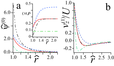
Figure 4: Against the dimensionless radial distance ${\hat{r}}$, we plot the dimensionless order parameter in the reference state ${\hat{\psi}}^{(0)}({\hat{r}})$ in (a), the dimensionless correlation length ${\hat{\xi}}$ in the reference state in the inset, and the $z$ component of the velocity field divided by that of the particle velocity $v_{z}^{(1)}/U$ at $\theta=\pi/2$ in (b) by setting the particle radius $r_{0}$ equal to $0.1\ \mu$m. The blue dashed, red solid, and green dash-dot curves are obtained by setting the reduced temperature $\tau$ equal to $1.82\times 10^{-4},4.05\times 10^{-4}$, and $2.82\times 10^{-3}$, respectively, under $h=1.55\times 10^{-2}\$cm${}^{3}/$s². The black dash-dot-dot curve is obtained for $\tau=4.05\times 10^{-4}$ and $h=1.73\times 10^{-1}\$cm${}^{3}/$s².

We obtain ${\hat{\psi}}^{(0)}$ by numerically solving Eq. (10) and the boundary conditions mentioned around this equation. In Fig. 4(a), ${\hat{\psi}}^{(0)}{({\hat{r}})}$ decreases as ${\hat{r}}$ increases. As $\tau$ decreases, the decrease is more gradual, i.e., the adsorption layer becomes thicker. The value of ${\hat{\psi}}^{(0)}(1)$ increases with $h$. We define ${\hat{\xi}}$ as $\xi/r_{0}\equiv{\hat{\omega}}^{-\nu}$, calculate its values in the reference state with the aid of the self-consistent condition, and plot the results in the inset of Fig. 4(a). The PA causes ${\hat{\xi}}<\xi_{\infty}/r_{0}={\hat{\tau}}^{-\nu}$ near the particle surface. For the force-free particle motion ($g=g_{0}$), we plot $v_{z}^{(1)}/U=-v_{\theta}^{(1)}/U$ at $\theta=\pi/2$ in Fig. 4(b). For a set of $(\tau,h)$, the plotted function changes its sign from positive to negative as ${\hat{r}}$ increases. Its zero is larger as $\tau$ decreases for $h=1.55\times 10^{-2}\$cm${}^{3}/$s². At $\tau=4.05\times 10^{-4}$, the curves for the different values of $h$ approximately coincide with each other. This property is also observed for each of the other values of $\tau$ although data not shown, and would appear because $\xi_{\infty}$ indicates the thickness of the adsorption layer. As required in our coarse-grained description, each curve in Fig. 4(b) can be well traced even if viewed with the local resolution provided by the corresponding local value of ${\hat{\xi}}$ shown in the inset of Fig. 4(a).

We write ${\bar{v}}_{n}$ for the partial volume per unit mass of the component $n$, and write ${\bar{v}}_{\pm}$ for $({\bar{v}}_{\rm a}\pm{\bar{v}}_{\rm b})/2$. If the mass densities are homogeneous, we have

$$\left.\frac{\partial\mu}{\partial\varphi}\right)_{T\rho}=\left.\frac{\partial\mu}{\partial P}\right)_{Tc_{\rm a}}\left.\frac{\partial P}{\partial\varphi}\right)_{T\rho}+\left.\frac{\partial\mu}{\partial c_{\rm a}}\right)_{TP}\left.\frac{\partial c_{\rm a}}{\partial\varphi}\right)_{T\rho}\ .$$ (14)

The LHS above equals $f_{\rm b}^{\prime\prime}(\psi)$, whereas the first and second derivatives of the first term on the RHS equal ${\bar{v}}_{-}$ and $f_{\rm b}^{\prime\prime}(\psi)\varphi$, respectively. Thus, with the aid of the identity $1={\bar{v}}_{\rm a}\rho_{\rm a}+{\bar{v}}_{\rm b}\rho_{\rm b}$, we obtain

$$\left.\frac{\partial\mu}{\partial c_{\rm a}}\right)_{TP}=2\rho_{\rm c}^{2}{\bar{v}}_{+{\rm c}}f_{\rm b}^{\prime\prime}(0)$$ (15)

far from the particle in the reference state. This can be substituted into Eq. (8). From the data in Table III of Ref. jaya , we estimate ${\bar{v}}_{\rm a}=1.03\times 10^{-3}\$m${}^{3}/$kg and ${\bar{v}}_{\rm b}=1.00\times 10^{-3}\$m${}^{3}/$kg for a mixture of LW lying in the homogeneous phase near the demixing critical point pipe . Thus, the mixture has ${\bar{v}}_{+{\rm c}}\approx 1/\rho_{\rm c}$. Because of $f_{\rm b}^{\prime\prime}(0)=k_{\rm B}TC_{1}\tau^{\gamma}/\xi_{0}^{2}$, we have $L_{*}=(\xi_{0}/r_{0})^{\eta}r_{0}/(6\pi\eta_{\rm s}C_{1})$.

For data points showing ${\cal M}\approx 50\ \mu$m²/s in Fig. 2, $h\psi^{(0)}(r_{0})$ should be larger than $6.63\times 10^{-7}\$kg/s², which value is calculated from ${\hat{\psi}}^{(0)}(1)$ for $\tau=2.82\times 10^{-3}$ and $h=1.55\times 10^{-2}\$cm³/s² in Fig. 4(a). Thus, the condition $\eta_{\rm s}\left|\varepsilon U\right|\ll\left|h\psi^{(0)}(r_{0})\right|$, mentioned in the main text, is satisfied if the particle speed is much smaller than $3\times 10^{2}\ \mu$m/s for the data points mentioned above. Considering that ${\hat{\psi}}^{(0)}(1)$ can be roughly approximated to be unity in Fig. 4(a), we can nondimensionalize the particle speed by dividing it by $h\psi_{*}/\eta_{\rm s}$ and use the dimensionless quotient as the smallness parameter.

References

- (1) B. V. Derjaguin, S. S. Dukhin, and V. V. Koptelova, “Capillary osmosis through porous partitions and properties of boundary layers of solutions,” J. Coll. Interf. Sci. 38, 584–595 (1972).
- (2) J. L. Anderson, M. E. Lowell, and D. C. Prieve, “Motion of a particle generated by chemical gradients part 1. non-electrolytes,” J. Fluid Mech. 117, 107–121 (1982).
- (3) J. L. Anderson and D. C. Prieve, “Diffusiophoresis: migration of colloidal particles in gradients of solute concentration,” Sep. Purif. Methods 13, 67–103 (1984).
- (4) D. C. Prieve and R. Roman, “Diffusiophoresis of a rigid sphere through a viscous electrolyte solution,” J. Chem. Soc., Faraday Trans. 2, 83, 1287–1306 (1987).
- (5) J. L. Anderson, “Colloid tranport by interfacial forces,” Ann. Rev. Fluid Mech. 21, 61–99 (1989).
- (6) P. O. Staffeld and J. A. Quinn, “Diffusion-induced banding of colloid particles via diffusiophoresis 2. non-electrolyte,” J. Coll. Interf. Sci. 130, 88–100 (1989).
- (7) B. Abécassis, C. Cottin-Bizonne, C. Ybert, A. Adjari and L. Bocquet, “Osmotic manipulation of particles for microfluidic applications,” New J. Phys. 11, 075022 (2009).
- (8) G. Volpe, I. Buttinoni, D. Vogt, H.-J. Kümmerer, and C. Bechinger, “Microswimmers in patterned environments,” Soft Matter 7, 8810 (2011).
- (9) C. Lee, C. Cottin-Bizonne, A.-L. Biance, P. Jpseph, L. Bocquet, and C. Ybert, “Osmotic flow through fully permeable nanochannels,” Phys. Rev. Lett. 112, 244501 (2014).
- (10) A. Kar, T.-Y. Chang, I. O. Riviera, A. Sen, and D. Velegol, “Enhanced transport into and out of dead-end pores,” ACS Nano 9, 746–753 (2015).
- (11) S. Shin, E. Urn, B. Sabass, J. T. Auit, M. Rahimi, P. B. Warren, and H. A. Stone, “Size-dependent control of colloid transport via solute gradients in dead-end channels,” Proc. Natl. Acad. Sci. USA 113, 257–261 (2016).
- (12) H. J. Keh, “Diffusiophoresis of charged particles and diffusioosmosis of electrolyte solutions,” Curr. Opin. Coll. Interf. Sci. 24, 13–22 (2016).
- (13) D. Velegol, A. Garg, R. Gusha, A. Kar, and M. Kumar, “Origins of concentration gradients for diffusiophoresis,” Soft Matter 12, 4686–4703 (2016).
- (14) S. Marbach and L. Bocquet, “Osmosis, from molecular insights to large-scale applications,” Chem. Soc. Rev. 48, 3102–3144 (2019).
- (15) S. Shin, “Diffusiophoretic separation of colloids in microfluidic flows,” Phys. Fluids 32, 101302 (2020).
- (16) S. Ramírez-Hinestrosa and D. Frenkel, “Challenges in modelling diffusiophoretic transport,” Eur. Phys. J. B 94, 199 (2021).
- (17) P. M. Vinze, A. Choudhary, and S. Pushpavanam, “Motion of an active particle in a linear concentration gradient,” Phys. Fluids 33, 032011 (2021).
- (18) R. Okamoto, Y. Fujitani, and S. Komura, “Drag coefficient of a rigid spherical particle in a near-critical binary fluid mixture,” J. Phys. Soc. Jpn 82, 084003 (2013).
- (19) A. Furukawa, A. Gambassi, S. Dietrich, and H. Tanaka, “Nonequilibrium critical Casimir effect in binary fluids,” Phys. Rev. Lett. 111, 055701 (2013).
- (20) J. W. Cahn, “Critical point wetting,” J. Chem. Phys. 66, 3667–3672 (1977).
- (21) D. Beysens and S. Leibler, “Observation of an anomalous adsorption in a critical binary mixture,” J. Physique Lett. 43, 133–136 (1982).
- (22) M. N. Binder, in Phase Transitions and Critical Phenomena VIII, edited by C. Domb and J. Lebowitz, “Critical behavior at surfaces” (Academic, London, 1983).
- (23) D. Beysens, and D. Estève, “Adsorption phenomena at the surface of silica spheres in a binary liquid mixture,” Phys. Rev. Lett. 54, 2123–2126 (1985).
- (24) R. Holyst and A. Poniewierski, “Wetting on a spherical surface,” Phys. Rev. B 36, 5628–5630 (1987).
- (25) H. W. Diehl, “The theory of boundary critical phenomena,” Int. J. Mod. Phys. B 11, 3503–3523 (1997).
- (26) D. Beysens, “Brownian motion in strongly fluctuating liquid,” Thermodyn. Interf. Fluid Mech. 3, 1–8 (2019).
- (27) Y. Fujitani, “Suppression of viscosity enhancement around a Brownian particle in a near-critical binary fluid mixture,” J. Fluid Mech. 907, A21 (2021).
- (28) S. Yabunaka and Y. Fujitani, “Drag coefficient of a rigid spherical particle in a near-critical binary fluid mixture, beyond the regime of the Gaussian model,” J. Fluid Mech. 886 A2 (2020).
- (29) M. E. Fisher, and H. Au-Yang, “Critical wall perturbations and a local free energy functional,” Physica A 101, 255–264 (1980).
- (30) R. Okamoto and A. Onuki, “Casimir amplitude and capillary condensation of near-critical binary fluids between parallel plates: renormalized local functional theory,” J. Chem. Phys. 136, 114704 (2012).
- (31) S. Yabunaka and A. Onuki, “Critical adsorption profiles around a sphere and a cylinder in a fluid at criticality: local functional theory,” Phys. Rev. E 96, 032127 (2017).
- (32) S. Yabunaka, R. Okamoto, and A. Onuki, “Hydrodynamics in bridging and aggregation of two colloidal particles in a near-critical binary mixture,” Soft Matter 11, 5738–5747 (2015).
- (33) Y. Fujitani, “Undulation amplitude of a fluid membrane in a near-critical binary fluid mixture calculated beyond the Gaussian model supposing weak preferential attraction,” J. Phys. Soc. Jpn. 86, 044602 (2017).
- (34) A. Pelisetto and E. Vicari, “Critical phenomena and renormalization-group theory,” Phys. Rep. 368, 549–727 (2002).
- (35) P. G. Wolynes, ”Osmotic effects near the critical point,” J. Phys. Chem. 80, 1570–1572 (1976).
- (36) S. Yabunaka and Y. Fujitani, “Isothermal transport of a near-critical binary fluid mixture through a capillary tube with the preferential adsorption,” Phys. Fluids 34, 052012 (2022).
- (37) P. C. Hohenberg and B. I. Halperin, “Theory of dynamic critical phenomena,” Rev. Mod. Phys. 49, 435–479 (1977).
- (38) A. Onuki, Phase Transition Dynamics (Cambridge University Press, Cambridge, 2002), Chap. 6.1.
- (39) A. Onuki, “Dynamic equations and bulk viscosity near the gas-liquid critical point,” Phys. Rev. E 55, 403–420 (1997).
- (40) K. Kawasaki, “Kinetic equations and time correlation functions of critical fluctuations,” Ann. Phys. (N. Y.) 61, 1–56 (1970).
- (41) J. V. Sengers, “Transport properties near critical points,” Int. J. Thermophys. 6, 203–232 (1985).
- (42) G. G. Stokes, “On the effect of the internal friction of fluid on the the motion of pendulums,” Trans. Camb. Phil. Soc. 9, 8–93 (1851).
- (43) W. Sutherland, “A dynamical theory of diffusion for nonelectrolytes and the molecular mass of albumin,” Phil. Mag. 9, 781–785 (1905).
- (44) A. Einstein, “Über die von der molekularkinetischen theorie der wärme geforderte bewegung von in ruhenden flüssigkeiten suspendierten teilchen,” Ann. Phys. (Leipzig) 322, 549–560 (1905).
- (45) Y. Fujitani, “Connection of fields across the interface in the fluid particle dynamics method for colloidal dispersion,” J. Phys. Soc. Jpn. 76, 064401 (2007).
- (46) S. Z. Mirzaev, R. Behrends, T. Heimburg, J. Haller, and U. Kaatze, “Critical behavior of 2,6-dimethylpyridine-water: Measurements of specific heat, dynamic light scattering, and shear viscosity,” J. Chem. Phys. 124 144517 (2006).
- (47) H. L Swinney and D. L. Henry, “Dynamics of fluids near the critical point: decay rate of order-parameter fluctuations,” Phys. Rev. A 8, 2586–2617 (1973).
- (48) N. Sharifi-Mood, J. Koplik, and C. Maldarelli, “Molecular dynamics simulation of the motion of colloidal nanoparticles in a solute concentration gradient and a comparison to the continuum limit,” Phys. Rev. Lett. 111, 184501 (2013).
- (49) Y. Fujitani, “Effective viscosity of a near-critical binary fluid mixture with colloidal particles dispersed dilutely under weak shear,” J. Phys. Soc. Jpn. 83, 084401.
- (50) Y. Jayalakshmi, J. S. van Duijneveldt, and D. Beysens, “Behavior of density and refractive index in mixtures of 2,6-lutidine and water,” J. Chem. Phys. 100, 604–609 (1994).
- (51) K. To, “Coexistence curve exponent of a binary mixture with a high molecular weight polymer,” Phys. Rev. E 63, 026108 (2001).
- (52) R. A. Omari, C. A. Grabowski & A. Mukhopadhyay, “Effect of surface curvature on critical adsorption,” Phys. Rev. Lett. 103, 225705 (2009).
- (53) A. Stein, S. J. Davidson, J. C. Allegra, and G. F. Allen, “Tracer diffusion and shear viscosity for the system 2,6-lutidine-water near the lower critical point,” J. Chem. Phys. 56 6164–6168 (1972).
- (54) C. A. Grattoni, R. A. Dawe, C. Y. Seah, and J. D. Gray, “Lower critical solution coexistence curve and physical properties (density, viscosity, surface tension, and interfacial tension) of 2,6-lutidinewater,” Chem. Eng. Data, 38, 516–519 (1993).