The Long-Moody construction and twisted Alexander invariants

Abstract.

In 1994, Long and Moody introduced a method to construct a new representation of the braid group from the representation of the braid group or the semidirect product of the braid group and the free group. In this paper, we show that its matrix presentation is written using the Fox derivative, and also a relation with twisted Alexander invariants.

1. Introduction

When we are given a representation of the braid group $B_{n}$, it is natural to hope to construct a link invariant from the representation since any link is obtained as the closure of a braid. For example, Burau [5] constructed a representation $\mathscr{B}\colon B_{n}\to GL_{n}(\mathbb{Z}[t^{\pm 1}])$ that reconstructs the Alexander polynomial. Specifically, let $\widetilde{\mathscr{B}}\colon B_{n}\to GL_{n-1}(\mathbb{Z}[t^{\pm 1}])$ be the reduced Burau representation and $b\in B_{n}$ an $n$-braid, then

$$\Delta_{\hat{b}}(t)=\pm t^{l}\frac{(t-1)\det(\widetilde{\mathscr{B}}(b)-I_{n-1})}{(t^{n}-1)},$$

where $l\in\mathbb{Z}$, $\Delta_{\hat{b}}(t)$ is the Alexander polynomial of the closure of $b$, and $I_{k}$ is the $k\times k$ identity matrix. Moreover, Birman [3] showed that the multivariable Alexander polynomial $\Delta_{\hat{b}}(t_{1},\ldots,t_{n})$ of the closure of a pure braid $b$ is described by the reduced Gassner representation $\widetilde{\mathscr{G}}\colon P_{n}\to GL_{n-1}(\mathbb{Z}[t_{1}^{\pm 1},\ldots,t_{n}^{\pm 1}])$ of the pure braid group $P_{n}$ as follows:

$$\Delta_{\hat{b}}(t_{1},\ldots,t_{n})=\pm t_{1}^{l_{1}}\cdots t_{n}^{l_{n}}\frac{\det(\widetilde{\mathscr{G}}(b)-I_{n-1})}{(t_{1}\cdots t_{n}-1)},$$

where $l_{1},\ldots,l_{n}\in\mathbb{Z}$.

As a generalization of the Alexander polynomial, Wada [15] and Lin [11] independently defined the twisted Alexander invariant which is an invariant of a given link and a representation of the fundamental group of the link complement. Conway [6] introduced the twisted Burau map $\mathscr{B}_{\rho}\colon B_{c}\to GL_{nk}(R[t_{1}^{\pm 1},\ldots,t_{\mu}^{\pm 1}])$, where $R$ is a commutative ring and $\rho\colon F_{n}\to GL_{k}(R)$ is a representation of the free group $F_{n}$. An $n$-braid $b$ is $\mu$-colored if each of its components is assigned an integer in $\{1,2,\ldots,\mu\}$. Then we obtain a sequence $c=(c_{1},\ldots,c_{n})$ of integers. For such a sequence $c=(c_{1},\ldots,c_{n})$, we can define the subgroup $B_{c}$ of $B_{n}$, which is called the $c$-colored braid group; see Section 3. The twisted Burau map is defined as a homomorphism of the twisted homology of the $n$-punctured disk, and generally not a representation. Conway showed an analogue of the above formulas, that is, the twisted Alexander invariant is obtained from the reduced twisted Burau map $\widetilde{\mathscr{B}}_{\rho}\colon B_{c}\to GL_{(n-1)k}(R[t_{1}^{\pm 1},\ldots,t_{\mu}^{\pm 1}])$: suppose that $F_{n}$ is generated by $x_{1},\ldots,x_{n}$ which are the standard generators of the fundamental group of the $n$-punctured disk. For a $\mu$-colored braid $b\in B_{c}$, if a representation $\rho\colon F_{n}\to GL_{k}(R)$ factors through a representation $\pi_{1}(S^{3}\setminus\hat{b})\to GL_{k}(R)$, then

$$\Delta_{\hat{b},\rho}(t_{1},\ldots,t_{\mu})=\pm\varepsilon t_{1}^{l_{1}}\cdots t_{\mu}^{l_{\mu}}\frac{\det(\widetilde{\mathscr{B}}_{\rho}(b)-I_{(n-1)k})}{\det(\rho(x_{1}\cdots x_{n})t_{c_{1}}\cdots t_{c_{n}}-I_{k})},$$

where $\varepsilon\in\det(\rho(\pi_{1}(S^{3}\setminus\hat{b})))$, $l_{1},\ldots,l_{\mu}\in\mathbb{Z}$, and $\Delta_{\hat{b},\rho}(t)$ is the twisted Alexander invariant of the closure of $b$ associated with the representation $\pi_{1}(S^{3}\setminus\hat{b})\to GL_{k}(R)$ induced by $\rho$.

On another note, Long and Moody [12] introduced a method of constructing a new representation of $B_{n}$ from a representation of $B_{n}\ltimes F_{n}$ or $B_{n+1}$, where the action of $B_{n}$ on $F_{n}$ is the Artin representation. This method is called the Long-Moody construction. More precisely, given a representation $\rho\colon B_{n}\ltimes F_{n}\to GL_{k}(R)$, its Long-Moody construction is an $nk$-dimensional representation of $B_{n}$. This representation is more complicated and abundant than the initial one. For example, if we take a one-dimensional trivial representation as the initial one, then we obtain the unreduced Burau representation. Bigelow and Tian [2] generalized this construction to some subgroups of $B_{n}$. Soulié also studied this construction from a functorial point of view and extended it in [13], and then generalized it to other families of groups, such as the mapping class group of surfaces [14] and the welded braid group [1] with Bellingeri.

In this paper, we introduce the multivariable reduced Long-Moody construction $\widetilde{\mathcal{LM}}_{\mathfrak{t}_{c}}(\rho)\colon B_{c}\to GL_{(n-1)k}(R[t_{1}^{\pm 1},\ldots,t_{\mu}^{\pm 1}])$ and show a relation with the twisted Alexander invariant. In section 2, we introduce the definition of the twisted Alexander invariant with reference to Wada [15]. In section 3, we recall the action of the braid group on the free group and explain the colored braids. In section 4, we define the multivariable Long-Moody construction which is a generalization of [2] and show that a matrix presentation of the Long-Moody construction is written by the Fox derivative. Then we give a formula related to the twisted Alexander invariant:

Theorem (Theorem 4.8).

Let $b\in B_{c}$ be a $\mu$-colored braid and $\hat{b}$ its closure. Let $\rho\colon B_{c}\ltimes F_{n}\to GL_{k}(R)$ be a representation such that the restriction $\rho|_{F_{n}}\colon F_{n}\to GL_{k}(R)$ factors through $\pi_{1}(S^{3}\setminus\hat{b})\to GL_{k}(R)$. Then

$$\Delta_{\hat{b},\rho}(t_{1},\ldots,t_{\mu})=\pm\varepsilon t_{1}^{l_{1}}\cdots t_{\mu}^{l_{\mu}}\frac{\det\left(\widetilde{\mathcal{LM}}_{\mathfrak{t}_{c}}(\rho)(b)-\mathrm{Diag}\left(\rho(b),\ldots,\rho(b)\right)\right)}{\det(\rho(x_{1}\cdots x_{n})t_{c_{1}}\cdots t_{c_{n}}-I_{k})}$$

for some $\varepsilon\in R^{\times}$ and $l_{1},\ldots,l_{\mu}\in\mathbb{Z}$.

In section 5, we give examples of the main theorem in the case of some knots: the trefoil knot, $(2,q)$-torus knot, and figure eight knot.

2. Twisted Alexander invariants

Let $G$ be a group with a finite presentation

$$G=\langle x_{1},\ldots,x_{n}\mid r_{1},\ldots,r_{m}\rangle$$

such that there exists a surjective homomorphism

$$\alpha\colon G\to H:=\mathbb{Z}^{\oplus\mu}\cong\langle t_{1},\ldots,t_{\mu}\mid t_{i}t_{j}=t_{j}t_{i}\ (1\leq i<j\leq\mu)\rangle.$$

Suppose that $G$ is the fundamental group of a $\mu$-component link complement, then we fix a homomorphism $\alpha\colon G\to H$ that maps the meridian of $i$-th component to $t_{i}$. Let $\rho\colon G\to GL_{k}(R)$ be a representation, where $R$ is a unique factorization domain. These maps are naturally extended to the ring homomorphisms $\widetilde{\alpha}\colon\mathbb{Z}[G]\to\mathbb{Z}[H]$ and $\widetilde{\rho}\colon\mathbb{Z}[G]\to M_{k}(R)$, where $M_{k}(R)$ is the matrix algebra of degree $k$ over $R$. Then the tensor product homomorphism $\widetilde{\rho}\otimes\widetilde{\alpha}\colon\mathbb{Z}[G]\to M_{k}(R[H])$ of $\widetilde{\rho}$ and $\widetilde{\alpha}$ is defined by

$$(\widetilde{\rho}\otimes\widetilde{\alpha})(g):=\rho(g)\alpha(g)$$

for any $g\in G$. Let $F_{n}$ be the free group generated by $x_{1},\ldots,x_{n}$ and $\phi\colon F_{n}\to G$ the surjective homomorphism induced by the presentations. Similarly to $\alpha$ and $\rho$, the homomorphism $\phi$ induces a ring homomorphism $\widetilde{\phi}\colon\mathbb{Z}[F_{n}]\to\mathbb{Z}[G]$. Then we obtain the ring homomorphism

$$\Phi:=(\widetilde{\rho}\otimes\widetilde{\alpha})\circ\widetilde{\phi}\colon\mathbb{Z}[F_{n}]\to M_{k}(R[H]).$$

We define the $m\times n$ matrix $M$ whose $(i,j)$ component is the $k\times k$ matrix

$$\Phi\left(\frac{\partial r_{i}}{\partial x_{j}}\right)\in M_{k}(R[H]),$$

where $\displaystyle\frac{\partial}{\partial x_{j}}$ is the Fox derivative with respect to $x_{j}$, that is, a linear map $\mathbb{Z}[F_{n}]\to\mathbb{Z}[F_{n}]$ over $\mathbb{Z}$ satisfying two conditions:

• $\displaystyle\frac{\partial x_{i}}{\partial x_{j}}=\delta_{ij}$, where $\delta_{ij}$ is the Kronecker delta, and

• $\displaystyle\frac{\partial(gg^{\prime})}{\partial x_{j}}=\displaystyle\frac{\partial g}{\partial x_{j}}+g\displaystyle\frac{\partial g^{\prime}}{\partial x_{j}}$ for any $g,g^{\prime}\in F_{n}$.

This matrix $M$ is called the Alexander matrix of the presentation of $G$ associated with the representation $\rho$.

For $1\leq j\leq n$, let $M_{j}$ be the $m\times(n-1)$ matrix obtained from $M$ by removing the $j$-th column. We regard $M_{j}$ as an $mk\times(n-1)k$ matrix with entries in $R[H]$. For an $(n-1)k$-tuple of indices

$$I=\left(i_{1},\ldots,i_{(n-1)k}\right)\ \ \left(1\leq i_{1}<\cdots<i_{(n-1)k}\leq mk\right),$$

we write $M^{I}_{j}$ for the $(n-1)k\times(n-1)k$ matrix consisting of the $i_{l}$-th rows of the matrix $M_{j}$, where $1\leq l\leq(n-1)k$.

We can see that there is an integer $1\leq i\leq n$ such that $\det\Phi(x_{i}-1)\neq 0$. Moreover, for such integers $i,j$ and any choice of the indices $I$, the following equality holds:

$$\det M^{I}_{i}\det\Phi(x_{j}-1)=\pm\det M^{I}_{j}\det\Phi(x_{i}-1).$$

Definition 2.1.

The twisted Alexander invariant $\Delta_{G,\rho}(t_{1},\ldots,t_{\mu})$ of the group $G$ associated with the representation $\rho$ is defined to be a rational expression

$$\Delta_{G,\rho}(t_{1},\ldots,t_{\mu}):=\frac{\gcd_{I}(\det M^{I}_{j})}{\det\Phi(x_{j}-1)}$$

provided that $\det\Phi(x_{j}-1)\neq 0$. This is well-defined up to a factor $\varepsilon t_{1}^{\l_{1}}\cdots t_{\mu}^{l_{\mu}}$, where $\varepsilon\in R^{\times}$ and $l_{1},\ldots,l_{\mu}\in\mathbb{Z}$. If $m<n-1$, we define $\Delta_{G,\rho}(t_{1},\ldots,t_{\mu}):=0$.

The twisted Alexander invariant is an invariant of the group $G$, the surjective homomorphism $\alpha$, and the representation $\rho$. More precisely, the twisted Alexander invariant is independent of the choice of the presentation of $G$. Furthermore, if two representations $\rho_{1}$ and $\rho_{2}$ are equivalent, then we have $\Delta_{G,\rho_{1}}(t_{1},\ldots,t_{\mu})\equiv\Delta_{G,\rho_{2}}(t_{1},\ldots,t_{\mu})$.

3. Colored braids

In this section, we make recollections on braid groups and their natural actions on free groups. We refer the reader to [8] for further details. Also we explain the notion of colored braid.

Let $B_{n}$ be the braid group of $n$ strands. This group has the following presentation, which is called the Artin presentation:

$$\left\langle\sigma_{1},\ldots,\sigma_{n-1}\mathrel{}\middle|\mathrel{}\begin{array}[]{ll}\sigma_{i}\sigma_{j}=\sigma_{j}\sigma_{i}&(|i-j|\geq 2)\\ \sigma_{i}\sigma_{i+1}\sigma_{i}=\sigma_{i+1}\sigma_{i}\sigma_{i+1}&(1\leq i\leq n-2)\end{array}\right\rangle.$$

The generator $\sigma_{i}$ corresponds to the $n$-braid described in Figure 1. There is a natural surjection from $B_{n}$ onto the symmetric group $S_{n}$. Its kernel $P_{n}$ is called the pure braid group.

Figure 1. The generator $\sigma_{i}$

Let $D^{2}$ be the unit 2-disk in $\mathbb{R}^{2}$ and fix $n$ distinct points $z_{1},\ldots,z_{n}$ in the interior of $D^{2}$. We shall assume so that each $z_{i}$ lies in $\textrm{Int}(D^{2})\cap(\mathbb{R}\times\{0\})=(-1,1)\times\{0\}$ and $z_{1}<\cdots<z_{n}$. Set $D_{n}:=D^{2}\setminus\{z_{1},\ldots,z_{n}\}$ and fix a base point $z\in\partial D_{n}$. Let $x_{i}$ be the simple loop around $z_{i}$ based at $z$ for $1\leq i\leq n$ in Figure 2.

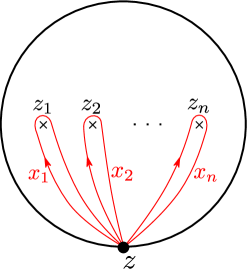
Figure 2. The $n$-punctured disk $D_{n}$ and the generators of its fundamental group

Then the fundamental group $\pi_{1}(D_{n},z)$ is identified with the free group $F_{n}=\left\langle x_{1},\ldots,x_{n}\right\rangle$. The braid group $B_{n}$ is isomorphic to the mapping class group $\mathcal{M}(D_{n})$ of $D_{n}$, which is the group of isotopy classes of orientation-preserving self-homeomorphisms of $D_{n}$ fixing the boundary pointwise. Since each element of $\mathcal{M}(D_{n})\cong B_{n}$ induces the automorphism of $\pi_{1}(D_{n},z)\cong F_{n}$ as described in Figure 3, we have a right action of $B_{n}$ on $F_{n}$ defined by

$$x_{j}\cdot\sigma_{i}:=\begin{cases}x_{i}x_{i+1}x_{i}^{-1}&(j=i)\\ x_{i}&(j=i+1)\\ x_{j}&(j\neq i,i+1)\end{cases}.$$

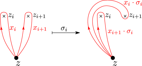
Figure 3. The action of $\sigma_{i}$ on $\pi_{1}(D_{n},z)$

For a braid $b\in B_{n}$, its closure $\hat{b}$ is the link in $S^{3}$ as described in Figure 4. Then the fundamental group $\pi_{1}(S^{3}\setminus\hat{b})$ of its complement admits a presentation as follows:

$$\left\langle x_{1},\ldots,x_{n}\mathrel{}\middle|\mathrel{}x_{1}=x_{1}\cdot b,\ldots,x_{n}=x_{n}\cdot b\right\rangle.$$

Figure 4. The closure of a braid

An $n$-braid $b$ is $\mu$-colored if each of its components is assigned an integer in $\{1,2,\ldots,\mu\}$ by a surjective map $\{1,2,\ldots,n\}\to\{1,2,\ldots,\mu\}$. Then we obtain a sequence $c=(c_{1},\ldots,c_{n})$ of integers, that is, $c_{i}\in\{1,2,\ldots,\mu\}\ (1\leq i\leq n)$ is the color of the $i$-th string. The color of a braid induces a coloring on the $n$ initial points and $n$ terminal points. The initial points are colored by the same as the sequence $c$, and let $c^{\prime}$ be the coloring on the terminal points. A $\mu$-colored braid is also called a $(c,c^{\prime})$-braid. If $b_{1}$ is a $(c,c^{\prime})$-braid and $b_{2}$ a $(c^{\prime},c^{\prime\prime})$-braid, then their composition $b_{1}b_{2}$ is a $(c,c^{\prime\prime})$-braid; see Figure 5. For any sequence $c$, the set $B_{c}$ is defined as the set of all $(c,c)$-braids. This set has a group structure and is a subgroup of $B_{n}$. The group $B_{c}$ is called the $c$-colored braid group. For example, $B_{(1,1,\ldots,1)}$ is equal to $B_{n}$ and $B_{(1,2,\ldots,n)}$ is equal to $P_{n}$.

Figure 5. $b_{1}$ is a $(c,c^{\prime})$-braid, $b_{2}$ is a $(c^{\prime},c^{\prime\prime})$-braid, and their composition $b_{1}b_{2}$ is a $(c,c^{\prime\prime})$-braid.

4. The Long-Moody construction

In this section, we introduce the multivariable Long-Moody construction for the $c$-colored braid group $B_{c}$ to describe a relation with the (multivariable) twisted Alexander invariant. This is a generalization of the one discussed in [2].

4.1. Definition

We fix a sequence $c=(c_{1},\ldots,c_{n})$ of integers $1,2,\ldots,\mu$, and set $H^{\prime}:=\langle t\rangle\oplus H\cong\mathbb{Z}^{\oplus\mu+1}$. We define a homomorphism $\mathfrak{t}_{c}\colon B_{c}\ltimes F_{n}\to H^{\prime}$ by the following:

$$\begin{cases}b=\sigma_{i_{1}}^{m_{1}}\cdots\sigma_{i_{l}}^{m_{l}}\mapsto t^{m_{1}+\cdots+m_{l}}&(b\in B_{c})\\ x_{j}\mapsto t_{c_{j}}&(j=1,\ldots,n)\end{cases}.$$

From [2, Theorem 3.1], we are able to apply the Long-Moody construction for a representation of $B_{c}\ltimes F_{n}$ that is a subgroup of $B_{n}\ltimes F_{n}$. Let $\rho\colon B_{c}\ltimes F_{n}\to GL_{k}(R)$ be a representation, where $R$ is a commutative ring. We regard $v\in R^{\oplus k}$ as a row vector $v=(v_{1},\ldots,v_{k})$, and thus the representation $\rho$ is multiplied from the right of $v$. Restricting $\rho$ and $\mathfrak{t}_{c}$ to the free group $F_{n}$ gives $R[H^{\prime}]^{\oplus k}$ a right $R[F_{n}]$-module structure. Then we consider a $R[H^{\prime}]$-module $R[H^{\prime}]^{\oplus k}\otimes_{R[F_{n}]}\mathcal{I}_{F_{n}}$, where $\mathcal{I}_{F_{n}}$ is the augmentation ideal of $F_{n}$, that is, $\mathcal{I}_{F_{n}}$ is the kernel of the augmentation $R[F_{n}]\to R$.

Definition 4.1.

The multivariable Long-Moody construction of the representation $\rho\colon B_{c}\ltimes F_{n}\to GL_{k}(R)$ is a representation $\mathcal{LM}_{\mathfrak{t}_{c}}(\rho)\colon B_{c}\to GL_{R[H^{\prime}]}(R[H^{\prime}]^{\oplus k}\otimes_{R[F_{n}]}\mathcal{I}_{F_{n}})$ given by

$$\mathcal{LM}_{\mathfrak{t}_{c}}(\rho)(b)(v\otimes h):=\bar{\mathfrak{t}}_{c}(b)\cdot\left(v\left((\rho\otimes\mathfrak{t}_{c})(b)\right)\otimes h\cdot b\right)$$

for any $b\in B_{c}$, $h\in\mathcal{I}_{F_{n}}$ and $v\in R[H^{\prime}]^{\oplus k}$, and the right action of $B_{c}$ on $F_{n}$ is naturally extended to the action on $\mathcal{I}_{F_{n}}$. Also, a homomorpshim $\bar{\mathfrak{t}}_{c}\colon B_{c}\to H^{\prime}$ is defined as $\bar{\mathfrak{t}}_{c}(b)=\mathfrak{t}_{c}(b)^{-1}$ for any $b\in B_{c}$.

By using the Fox derivative, we are able to calculate a matrix presentation for the Long-Moody construction:

Theorem 4.2.

For any $b\in B_{c}$,

$$\mathcal{LM}_{\mathfrak{t}_{c}}(\rho)(b)=\mathrm{Diag}\left(\rho(b),\ldots,\rho(b)\right)\cdot\left((\rho\otimes\mathfrak{t}_{c})\left(\frac{\partial(x_{i}\cdot b)}{\partial x_{j}}\right)\right)_{1\leq i,j\leq n}.$$

Proof.

Note that $\mathcal{I}_{F_{n}}$ is isomorphic to the free $R[F_{n}]$-module of rank $n$ generated by $x_{i}-1$ $(1\leq i\leq n)$. Therefore, there is an isomorphism

$$\begin{array}[]{ccc}R[H^{\prime}]^{\oplus k}\otimes_{R[F_{n}]}\mathcal{I}_{F_{n}}&\to&\displaystyle{\bigoplus_{i=1}^{n}}R[H^{\prime}]^{\oplus k}\vspace{5pt}\\ v\otimes(x_{i}-1)&\mapsto&0\oplus\cdots\oplus\underbrace{v}_{i-th}\oplus\cdots\oplus 0,\end{array}$$

and $GL_{R[H^{\prime}]}(R[H^{\prime}]^{\oplus k}\otimes_{R[F_{n}]}\mathcal{I}_{F_{n}})\cong GL_{nk}(R[H^{\prime}])$. Hence, for any $v_{1},\ldots,v_{n}\in R[H^{\prime}]^{\oplus k}$, we identify $v_{1}\oplus\cdots\oplus v_{n}\in\displaystyle{\bigoplus_{i=1}^{n}}R[H^{\prime}]^{\oplus k}$ with

$$(v_{1}\otimes(x_{1}-1))+\cdots+(v_{n}\otimes(x_{n}-1))\in R[H^{\prime}]^{\oplus k}\otimes_{R[F_{n}]}\mathcal{I}_{F_{n}}.$$

By the fundamental formula of the Fox derivative,

$$w-1=\sum^{n}_{j=1}\frac{\partial w}{\partial x_{j}}(x_{j}-1)$$

for any $w\in\mathbb{Z}[F_{n}]$. Hence

$$\mathcal{LM}_{\mathfrak{t}_{c}}(\rho)(b)(v\otimes(x_{i}-1)) =\bar{\mathfrak{t}}_{c}(b)\cdot\left(v\left((\rho\otimes\mathfrak{t}_{c})(b)\right)\otimes(x_{i}-1)\cdot b\right)$$

$$=\mathfrak{t}_{c}(b)^{-1}\cdot\mathfrak{t}_{c}(b)\cdot v(\rho(b))\otimes\sum^{n}_{j=1}\left(\frac{\partial(x_{i}\cdot b)}{\partial x_{j}}\right)(x_{j}-1)$$

$$=v(\rho(b))\otimes\sum^{n}_{j=1}\left(\frac{\partial(x_{i}\cdot b)}{\partial x_{j}}\right)(x_{j}-1)$$

$$=\sum^{n}_{j=1}v\left(\rho(b)\right)\left((\rho\otimes\mathfrak{t}_{c})\left(\frac{\partial(x_{i}\cdot b)}{\partial x_{j}}\right)\right)\otimes(x_{j}-1).$$

Therefore, we obtain the desired matrix presentation. ∎

By the above theorem. since we consider the product with the “inverse” homomorphism $\bar{\mathfrak{t}}_{c}$, the variable $t$ vanishes in the image of $\mathcal{LM}_{\mathfrak{t}_{c}}(\rho)$. Therefore, $\mathcal{LM}_{\mathfrak{t}_{c}}(\rho)$ can be regarded as a representation on $GL_{R[H]}(R[H]^{\oplus k}\otimes_{R[F_{n}]}\mathcal{I}_{F_{n}})\cong GL_{nk}(R[H])$. If $c=(1,1,\ldots,1)$, then this is a representation of $B_{n}$ which is equivalent to the representation of [12, Corollary 2.6]. Also, the case of $c=(1,2,\ldots,n)$ is just as a representation of $P_{n}$ of [2, Theorem 4.1].

Example 4.3.

Consider the one-dimensional trivial representation $\mathcal{T}\colon B_{c}\ltimes F_{n}\to GL_{1}(\mathbb{Z})$. Then the multivariable Long-Moody construction $\mathcal{LM}_{\mathfrak{t}_{c}}(\mathcal{T})\colon B_{c}\to GL_{n}(\mathbb{Z}[t_{1}^{\pm 1},\ldots,t_{\mu}^{\pm 1}])$ can be defined. If $c=(1,1,\ldots,1)$, this is equivalent to the unreduced Burau representation. Also, if $c=(1,2,\ldots,n)$, this is equivalent to the unreduced Gassner representation (cf. [2, Section 4]).

Remark 4.4.

The original Long-Moody construction [12, Theorem 2.1] is defined for $B_{n}$ without the homomorphism $\mathfrak{t}_{c}$. In other words, the Long-Moody construction of the representation $\rho\colon B_{n}\ltimes F_{n}\to GL_{k}(R)$ is a representation $\mathcal{LM}(\rho)\colon B_{n}\to GL_{R}(R^{\oplus k}\otimes_{R[F_{n}]}\mathcal{I}_{F_{n}})\cong GL_{nk}(R)$ given by

$$\mathcal{LM}(\rho)(b)(v\otimes h):=v(\rho(b))\otimes h\cdot b.$$

Moreover, this construction is also defined for the braid group $B_{n+1}$ via two “canonical” homomorphisms $F_{n}\to B_{n+1}$ and $B_{n}\to Aut(F_{n})$; see [12, Theorem 2.4]. Soulié [13, 14] extended and generalized this method. For example, if we choose homomorphisms $\chi\colon F_{n}\to B_{n+1}$ and $\kappa\colon B_{n}\to Aut(F_{n})$ satisfying the equation

$$\chi(x_{j})\sigma_{i+1}=\sigma_{i+1}\chi(\kappa(\sigma_{i})(x_{j})),$$

then the Long-Moody construction can be defined. Since this construction depends on $\chi$ and $\kappa$, we may write it as $\mathcal{LM}_{\kappa,\chi}\colon B_{n}\to GL_{R}(R^{\oplus k}\otimes_{R[F_{n}]}\mathcal{I}_{F_{n}})$ in this case. Also, Bellingeri and Soulié [1] defined this contruction for the welded braid group $WB_{n}$ which is a generalization of the braid group.

4.2. Reduced version

In order to describe a relation with the twisted Alexander invariant, we also consider other generators $g_{1},\ldots,g_{n}$ of $F_{n}$, where $g_{i}:=x_{1}\cdots x_{i}$; see Figure 6. The action of $B_{n}$ on this new generating set is given by

$$g_{j}\cdot\sigma_{i}:=\begin{cases}g_{j}&(j\neq i)\\ g_{i+1}g_{i}^{-1}g_{i-1}&(j=i\neq 1)\\ g_{2}g_{1}^{-1}&(j=i=1)\end{cases}.$$

Since the augmentation ideal $\mathcal{I}_{F_{n}}$ is also generated by $g_{i}-1\ (1\leq i\leq n)$, we have another matrix presentation of $\mathcal{LM}_{\mathfrak{t}_{c}}(\rho)(b)$ with respect to this generating set. Moreover $g_{n}$ is fixed by the action of $B_{n}$, and thus the matrix is written as

$$\mathcal{LM}_{\mathfrak{t}_{c}}(\rho)(b)=\mathrm{Diag}\left(\rho(b),\ldots,\rho(b)\right)\cdot\left(\begin{array}[]{cc}\left((\rho\otimes\mathfrak{t}_{c})\left(\displaystyle\frac{\partial(g_{i}\cdot b)}{\partial g_{j}}\right)\right)_{1\leq i,j\leq n-1}&V\\ 0&I_{k}\end{array}\right),$$

where $V$ is some $(n-1)k\times k$ matrix.

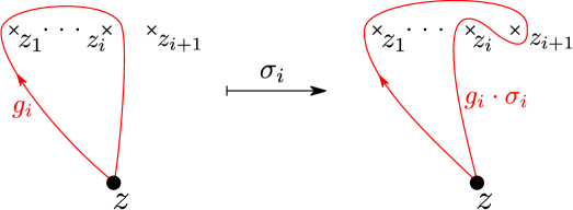
Figure 6. The generator $g_{i}$ and the action of $\sigma_{i}$

Definition 4.5.

Regard $F_{n-1}$ as being generated by $g_{1},\ldots,g_{n-1}$. The reduced multivariable Long-Moody construction of the representation $\rho$ is a representation $\widetilde{\mathcal{LM}}_{\mathfrak{t}_{c}}(\rho)\colon B_{n}\to GL_{R[H]}(R[H]^{\oplus k}\otimes_{R[F_{n-1}]}\mathcal{I}_{F_{n-1}})\cong GL_{(n-1)k}(R[H])$ given by

$$\widetilde{\mathcal{LM}}_{\mathfrak{t}_{c}}(\rho)(b)(v\otimes h):=\bar{\mathfrak{t}}_{c}(b)\cdot\left(v\left((\rho\otimes\mathfrak{t}_{c})(b)\right)\otimes h\cdot b\right)$$

for any $b\in B_{n}$, $h\in\mathcal{I}_{F_{n-1}}$ and $v\in R[H]^{\oplus k}$.

Its matrix presentation with respect to the basis $\left\{g_{i}-1\mathrel{}\middle|\mathrel{}1\leq i\leq n-1\right\}$ is

$$\widetilde{\mathcal{LM}}_{\mathfrak{t}_{c}}(\rho)(b)=\mathrm{Diag}\left(\rho(b),\ldots,\rho(b)\right)\cdot\left((\rho\otimes\mathfrak{t}_{c})\left(\frac{\partial(g_{i}\cdot b)}{\partial g_{j}}\right)\right)_{1\leq i,j\leq n-1}.$$

Example 4.6.

For the one-dimensional trivial representation $\mathcal{T}\colon B_{c}\ltimes F_{n}\to GL_{1}(\mathbb{Z})$, the multivariable reduced Long-Moody construction $\widetilde{\mathcal{LM}}_{\mathfrak{t}_{c}}(\mathcal{T})\colon B_{c}\to GL_{n-1}(\mathbb{Z}[t_{1}^{\pm 1},\ldots,t_{\mu}^{\pm 1}])$ is equivalent to the reduced Burau representation if $c=(1,1,\ldots,1)$, and equivalent to the reduced Gassner representation if $c=(1,2,\ldots,n)$.

Remark 4.7.

The Long-Moody construction has an interpretation as the twisted homology. Fix a sequence $c=(c_{1},\ldots,c_{n})$ of integers $1,2,\ldots,\mu$. Consider the surjection $\varphi_{c}\colon\pi_{1}(D_{n},z)\to H$ given by $\varphi_{c}(x_{i})=t_{c_{i}}$ for $1\leq i\leq n$. Note that $\varphi_{c}$ is equal to $\mathfrak{t}_{c}|_{F_{n}}$. Let $p\colon\widetilde{D}_{n}\to D_{n}$ be the universal covering of $D_{n}$ and set $\widetilde{z}:=p^{-1}(z)$. Let $\rho\colon B_{c}\ltimes\pi_{1}(D_{n},z)\left(\cong B_{c}\ltimes F_{n}\right)\to GL_{k}(R)$ be a representation. By identifying $R^{\oplus k}\otimes_{R}R[H]\cong R[H]^{\oplus k}$ and restricting $\rho$ to $\pi_{1}(D_{n},z)$, we obtain the representation $\rho\otimes\varphi_{c}\colon\pi_{1}(D_{n},z)\to GL_{k}(R[H])$. Then the chain complex of $R[H]$-modules

$$C_{*}^{\rho\otimes\varphi_{c}}(D_{n},z;R[H]^{\oplus k}):=R[H]^{\oplus k}\otimes_{\mathbb{Z}[\pi_{1}(D_{n},z)]}C_{*}(\widetilde{D}_{n},\widetilde{z})$$

and the twisted homology group $H_{*}^{\rho\otimes\varphi_{c}}(D_{n},z;R[H]^{\oplus k})$ are defined. From [6, Lemma 2.2], the $R[H]$-module $H_{1}^{\rho\otimes\varphi_{c}}(D_{n},z;R[H]^{\oplus k})$ is free of rank $nk$. As we have a representation $\rho|_{B_{n}}\colon B_{n}\to GL_{k}(R)$, the action $B_{n}\to Aut_{R[H]}(H_{1}^{\rho\otimes\varphi_{c}}(D_{n},z;R[H]^{\oplus k}))\cong GL_{nk}(R[H])$ is well-defined, and it is equivalent to the multivariable Long-Moody construction $\mathcal{LM}_{\mathfrak{t}_{c}}(\rho)\colon B_{c}\to GL_{nk}(R[H])$.

On the other hand, Conway [6] defined the twisted Burau map as a homomorphism on the twisted homology. Namely, let $\rho\colon\pi_{1}(D_{n},z)\to GL_{k}(R)$ be a representation and $b$ a $(c,c)$-colored braid, then the braid $b$ induces a well-defined homomorphism

$$\mathscr{B}_{\rho}(b)\colon H_{1}^{b(\rho\otimes\varphi_{c})}(D_{n},z;R[H]^{\oplus k})\to H_{1}^{\rho\otimes\varphi_{c}}(D_{n},z;R[H]^{\oplus k}).$$

From the above isomorphism of the twisted homology, we obtain the map $\mathscr{B}_{\rho}\colon B_{c}\to GL_{nk}(R[H])$, which is generally not a representation. Its matrix presentation is of the form

$$\mathscr{B}_{\rho}(b)=\left((\rho\otimes\varphi_{c})\left(\frac{\partial(x_{i}\cdot b)}{\partial x_{j}}\right)\right)_{1\leq i,j\leq n}.$$

In the setting above, we are able to consider the twisted homology group $H_{*}^{\rho\otimes\varphi_{c}}(D_{n};R[H]^{\oplus k})$ and an action of $B_{n}$ on $H_{1}^{\rho\otimes\varphi_{c}}(D_{n};R[H]^{\oplus k})$. Conway [6, Section 3.2] studied this group in detail. However, there is no obvious basis so that we are able to compute a matrix of $\widetilde{\mathcal{LM}}_{\mathfrak{t}_{c}}(\rho)$.

4.3. Relation with the twisted Alexander invariant

Conway [6, Theorem 3.15] proved a relation with the reduced twisted Burau map and the twisted Alexander invariant. The following theorem shows a relation with the multivariable reduced Long-Moody construction and the twisted Alexander invariant.

Theorem 4.8.

Let $b\in B_{c}$ be a $\mu$-colored braid and $\hat{b}$ its closure. Let $\rho\colon B_{c}\ltimes F_{n}\to GL_{k}(R)$ be a representation such that the restriction $\rho|_{F_{n}}\colon F_{n}\to GL_{k}(R)$ factors through the homomorphism $\phi$ and a representation $\pi_{1}(S^{3}\setminus\hat{b})\to GL_{k}(R)$. In other words, we assume the following diagram is commutative:

Then

$$\Delta_{\hat{b},\rho}(t_{1},\ldots,t_{\mu})=\pm\varepsilon t_{1}^{l_{1}}\cdots t_{\mu}^{l_{\mu}}\frac{\det\left(\widetilde{\mathcal{LM}}_{\mathfrak{t}_{c}}(\rho)(b)-\mathrm{Diag}\left(\rho(b),\ldots,\rho(b)\right)\right)}{\det(\rho(x_{1}\cdots x_{n})t_{c_{1}}\cdots t_{c_{n}}-I_{k})}$$

for some $\varepsilon\in R^{\times}$ and $l_{1},\ldots,l_{\mu}\in\mathbb{Z}$, where the representation $\pi_{1}(S^{3}\setminus\hat{b})\to GL_{k}(R)$ is induced by $\rho|_{F_{n}}$, and let the same symbol $\rho$ denote this representation.

Proof.

Recall the presentation of $\pi_{1}(S^{3}\setminus\hat{b})$ using the braid action in Section 3. Replacing the generators $x_{1},\ldots,x_{n}$ with $g_{1},\ldots,g_{n}$, $\pi_{1}(S^{3}\setminus\hat{b})$ also has a similar presentation:

$$\left\langle g_{1},\ldots,g_{n}\mathrel{}\middle|\mathrel{}g_{1}=g_{1}\cdot b,\ldots,g_{n-1}=g_{n-1}\cdot b\right\rangle.$$

Then the surjective homomorphism $\alpha\colon\pi_{1}(S^{3}\setminus\hat{b})\to H$ is given by $g_{i}\mapsto t_{c_{1}}\cdots t_{c_{i}}$ for $1\leq i\leq n$. Computing the Alexander matrix of this presentation, we have

$$M=\left(\Phi\left(\frac{\partial(g_{i}\cdot b)}{\partial g_{j}}\right)-\delta_{ij}I_{k}\right)_{1\leq i\leq n-1,1\leq j\leq n}.$$

Hence the twisted Alexander invariant is

$$\Delta_{\hat{b},\rho}(t)=\frac{\det M_{n}}{\det\Phi(g_{n}-1)}=\frac{\det\left(\Phi\left(\displaystyle\frac{\partial(g_{i}\cdot b)}{\partial g_{j}}\right)-I_{(n-1)k}\right)}{\det\Phi(g_{n}-1)}.$$

On the other hand, since $\Phi=(\widetilde{\rho}\otimes\widetilde{\alpha})\circ\widetilde{\phi}$, $\mathfrak{t}_{c}|_{F_{n}}=\alpha\circ\phi$ and $\rho|_{F_{n}}=\rho\circ\phi$, we have

$$\widetilde{\mathcal{LM}}_{\mathfrak{t}_{c}}(\rho)(b) =\mathrm{Diag}\left(\rho(b),\ldots,\rho(b)\right)\cdot\left((\rho\otimes\mathfrak{t}_{c})\left(\frac{\partial(g_{i}\cdot b)}{\partial g_{j}}\right)\right)$$

$$=\mathrm{Diag}\left(\rho(b),\ldots,\rho(b)\right)\cdot\left(\Phi\left(\frac{\partial(g_{i}\cdot b)}{\partial g_{j}}\right)\right).$$

Therefore

$$\det\left(\widetilde{\mathcal{LM}}_{\mathfrak{t}_{c}}(\rho)(b)-\mathrm{Diag}\left(\rho(b),\ldots,\rho(b)\right)\right)$$

$$= \det\mathrm{Diag}\left(\rho(b),\ldots,\rho(b)\right)\det\left((\rho\otimes\mathfrak{t}_{c})\left(\frac{\partial(g_{i}\cdot b)}{\partial g_{j}}\right)-I_{(n-1)k}\right)$$

$$= (\det\rho(b))^{n-1}\det\left(\Phi\left(\frac{\partial(g_{i}\cdot b)}{\partial g_{j}}\right)-I_{(n-1)k}\right)$$

and

$$\det(\rho(x_{1}\cdots x_{n})t_{c_{1}}\cdots t_{c_{n}}-I_{k}) =\det((\rho\otimes\mathfrak{t}_{c})(g_{n})-I_{k})=\det\Phi(g_{n}-1).$$

Since $\det\rho(b)\in R^{\times}$, the theorem holds. ∎

5. Examples

In this section, we give some examples of Theorem 4.8. The theorem supposes that a representation $\rho\colon B_{c}\ltimes F_{n}\to GL_{k}(R)$ satisfies the condition. Conversely, let us choose a representation $\rho\colon\pi_{1}(S^{3}\setminus\hat{b})\to GL_{k}(R)$ that extends to $B_{c}\ltimes F_{n}$ in the following examples.

Example 5.1.

([15, Section 4]) Set $b:=\sigma_{1}^{3}\in B_{2}=B_{(1,1)}$. Its closure is the trefoil knot $3_{1}$; see Figure 7.

Figure 7. The braid $\sigma_{1}^{3}$ and the trefoil knot $3_{1}$

Then

$$\pi_{1}(S^{3}\setminus\hat{b}) \cong\left\langle x_{1},x_{2}\mathrel{}\middle|\mathrel{}x_{1}=x_{1}\cdot b,x_{2}=x_{2}\cdot b\right\rangle$$

$$\cong\left\langle x_{1},x_{2}\mathrel{}\middle|\mathrel{}x_{1}x_{2}x_{1}=x_{2}x_{1}x_{2}\right\rangle$$

$$\cong\left\langle g_{1},g_{2}\mathrel{}\middle|\mathrel{}g_{1}=g_{1}\cdot b\right\rangle.$$

Let $\rho:=\widetilde{\mathscr{B}}\colon\pi_{1}(S^{3}\setminus\hat{b})(\cong B_{3})\to GL_{2}(\mathbb{Z}[s^{\pm 1}])$ be the reduced Burau representation given by

$$\rho(x_{1})=\left(\begin{array}[]{cc}-s&1\\ 0&1\end{array}\right)\ \ \textrm{and}\ \ \rho(x_{2})=\left(\begin{array}[]{cc}1&0\\ s&-s\end{array}\right).$$

This is naturally extended to $F_{2}$. The group $B_{2}\ltimes F_{2}$ has the following presentation:

$$\left\langle x_{1},x_{2},\sigma_{1}\mathrel{}\middle|\mathrel{}x_{1}\sigma_{1}=\sigma_{1}x_{1}x_{2}x_{1}^{-1},x_{2}\sigma_{1}=\sigma_{1}x_{1}\right\rangle,$$

and then if we set

$$\rho(\sigma_{1}):=\left(\begin{array}[]{cc}0&1\\ -1&1\end{array}\right),$$

the representation $\rho\colon B_{2}\ltimes F_{2}\to GL_{2}(\mathbb{Z}[s^{\pm 1}])$ is well-defined. Since $g_{1}\cdot b=g_{2}^{2}g_{1}^{-1}g_{2}^{-1}$, we have

$$\frac{\partial(g_{1}\cdot b)}{\partial g_{1}}=-g_{2}^{2}g_{1}^{-1}.$$

Therefore

$$\widetilde{\mathcal{LM}}_{\mathfrak{t}_{c}}(\rho)(b)=-\rho(b)\rho(g_{2}^{2}g_{1}^{-1})t^{3}=\left(\begin{array}[]{cc}st^{3}&-st^{3}+s^{2}t^{3}\\ st^{3}&-st^{3}\\ \end{array}\right),$$

and thus we obtain

$$\det\left(\widetilde{\mathcal{LM}}_{\mathfrak{t}_{c}}(\rho)(b)-\rho(b)\right)=\det\left(\begin{array}[]{cc}1+st^{3}&-st^{3}+s^{2}t^{3}\\ st^{3}&1-st^{3}\\ \end{array}\right)=1-s^{3}t^{6}$$

and

$$\det\left(\rho(x_{1}x_{2})t^{2}-I_{2}\right)=\det\left(\begin{array}[]{cc}-1&-st^{2}\\ st^{2}&-st^{2}-1\\ \end{array}\right)=1+st^{2}+s^{2}t^{4}.$$

Hence

$$\Delta_{\hat{b},\rho}(t)=\frac{1-s^{3}t^{6}}{1+st^{2}+s^{2}t^{4}}=1-st^{2}.$$

Example 5.2.

Set $b:=\sigma_{1}\sigma_{2}^{-1}\sigma_{1}\sigma_{2}^{-1}\in B_{3}=B_{(1,1,1)}$. Its closure is the figure eight knot $4_{1}$; see Figure 8.

Figure 8. The braid $\sigma_{1}\sigma_{2}^{-1}\sigma_{1}\sigma_{2}^{-1}$ and the figure eight knot $4_{1}$

Then

$$\pi_{1}(S^{3}\setminus\hat{b}) \cong\left\langle x_{1},x_{2},x_{3}\mathrel{}\middle|\mathrel{}x_{1}=x_{1}\cdot b,x_{2}=x_{2}\cdot b,x_{3}=x_{3}\cdot b\right\rangle$$

$$\cong\left\langle x_{2},x_{3}\mathrel{}\middle|\mathrel{}x_{2}[x_{3}^{-1},x_{2}]=[x_{3}^{-1},x_{2}]x_{3}\right\rangle$$

$$\cong\left\langle g_{1},g_{2},g_{3}\mathrel{}\middle|\mathrel{}g_{1}=g_{1}\cdot b,g_{2}=g_{2}\cdot b\right\rangle,$$

where $[x,y]:=xyx^{-1}y^{-1}$. Let $\rho\colon\pi_{1}(S^{3}\setminus\hat{b})\to SL_{2}(\mathbb{Z}_{7})$ be the representation given by

$$\rho(x_{1})=\left(\begin{array}[]{cc}2&0\\ 0&4\end{array}\right),\ \ \rho(x_{2})=\left(\begin{array}[]{cc}1&1\\ 4&5\end{array}\right)\ \ \textrm{and}\ \ \rho(x_{3})=\left(\begin{array}[]{cc}1&2\\ 2&5\end{array}\right).$$

The group $B_{3}\ltimes F_{3}$ has a presentation

$$\left\langle x_{1},x_{2},x_{3},\sigma_{1},\sigma_{2}\mathrel{}\middle|\mathrel{}\begin{array}[]{l}x_{1}\sigma_{1}=\sigma_{1}x_{1}x_{2}x_{1}^{-1},x_{2}\sigma_{1}=\sigma_{1}x_{1},x_{3}\sigma_{1}=\sigma_{1}x_{3},\\ x_{1}\sigma_{2}=\sigma_{2}x_{1},x_{2}\sigma_{2}=\sigma_{2}x_{2}x_{3}x_{2}^{-1},x_{3}\sigma_{2}=\sigma_{2}x_{2},\\ \sigma_{1}\sigma_{2}\sigma_{1}=\sigma_{2}\sigma_{1}\sigma_{2}\end{array}\right\rangle,$$

and setting

$$\rho(\sigma_{1})=\left(\begin{array}[]{cc}5&5\\ 5&1\end{array}\right)\ \ \textrm{and}\ \ \rho(\sigma_{2})=\left(\begin{array}[]{cc}4&0\\ 0&2\end{array}\right),$$

the representation $\rho$ is extended to $B_{3}\ltimes F_{3}$. From $g_{1}\cdot b=g_{1}g_{2}^{-1}g_{3}g_{1}^{-1}g_{3}^{-1}g_{2}g_{1}^{-1}g_{3}g_{1}g_{3}^{-1}g_{2}g_{1}^{-1}$ and $g_{2}\cdot b=g_{1}g_{2}^{-1}g_{3}g_{1}^{-1}g_{3}^{-1}g_{2}g_{1}^{-1}g_{3}$,

$$\begin{split}\frac{\partial(g_{1}\cdot b)}{\partial g_{1}}&=1-g_{1}g_{2}^{-1}g_{3}g_{1}^{-1}-g_{1}g_{2}^{-1}g_{3}g_{1}^{-1}g_{3}^{-1}g_{2}g_{1}^{-1}\\ &\quad\quad+g_{1}g_{2}^{-1}g_{3}g_{1}^{-1}g_{3}^{-1}g_{2}g_{1}^{-1}g_{3}-g_{1}g_{2}^{-1}g_{3}g_{1}^{-1}g_{3}^{-1}g_{2}g_{1}^{-1}g_{3}g_{1}g_{3}^{-1}g_{2}g_{1}^{-1},\\ \frac{\partial(g_{1}\cdot b)}{\partial g_{2}}&=-g_{1}g_{2}^{-1}+g_{1}g_{2}^{-1}g_{3}g_{1}^{-1}g_{3}^{-1}+g_{1}g_{2}^{-1}g_{3}g_{1}^{-1}g_{3}^{-1}g_{2}g_{1}^{-1}g_{3}g_{1}g_{3}^{-1},\\ \frac{\partial(g_{2}\cdot b)}{\partial g_{1}}&=1-g_{1}g_{2}^{-1}g_{3}g_{1}^{-1}-g_{1}g_{2}^{-1}g_{3}g_{1}^{-1}g_{3}^{-1}g_{2}g_{1}^{-1},\\ \frac{\partial(g_{2}\cdot b)}{\partial g_{2}}&=-g_{1}g_{2}^{-1}+g_{1}g_{2}^{-1}g_{3}g_{1}^{-1}g_{3}^{-1}.\end{split}$$

Therefore

$$\widetilde{\mathcal{LM}}_{\mathfrak{t}_{c}}(\rho)(b) =\left(\begin{array}[]{cc}\rho(b)&0\\ 0&\rho(b)\\ \end{array}\right)\left(\begin{array}[]{cc}(\rho\otimes\mathfrak{t}_{c})\left(\displaystyle\frac{\partial(g_{1}\cdot b)}{\partial g_{1}}\right)&(\rho\otimes\mathfrak{t}_{c})\left(\displaystyle\frac{\partial(g_{1}\cdot b)}{\partial g_{2}}\right)\\ (\rho\otimes\mathfrak{t}_{c})\left(\displaystyle\frac{\partial(g_{2}\cdot b)}{\partial g_{1}}\right)&(\rho\otimes\mathfrak{t}_{c})\left(\displaystyle\frac{\partial(g_{2}\cdot b)}{\partial g_{2}}\right)\\ \end{array}\right)$$

$$=\left(\begin{array}[]{cccc}\displaystyle\frac{5t^{3}+3t^{2}+6t+5}{t}&\displaystyle\frac{5t^{3}+t^{2}+5}{t}&\displaystyle\frac{4t^{2}+5t+1}{t^{2}}&\displaystyle\frac{t^{2}+3t+1}{t^{2}}\\ \displaystyle\frac{5t^{3}+4t^{2}+5}{t}&\displaystyle\frac{t^{3}+2t^{2}+6t+1}{t}&\displaystyle\frac{4t^{2}+6t+4}{t^{2}}&\displaystyle\frac{3t^{2}+t+5}{t^{2}}\\ \displaystyle\frac{t^{2}+6t+5}{t}&\displaystyle\frac{t^{2}+5}{t}&\displaystyle\frac{5t+1}{t^{2}}&\displaystyle\frac{3t+1}{t^{2}}\\ \displaystyle\frac{4t^{2}+5}{t}&\displaystyle\frac{5t^{2}+6t+1}{t}&\dfrac{6t+4}{t^{2}}&\displaystyle\frac{t+5}{t^{2}}\\ \end{array}\right).$$

Hence

$$\det\left(\widetilde{\mathcal{LM}}_{\mathfrak{t}_{c}}(\rho)(b)-\left(\begin{array}[]{cc}\rho(b)&0\\ 0&\rho(b)\\ \end{array}\right)\right)$$

$$= \det\left(\begin{array}[]{cccc}\displaystyle\frac{5t^{3}+3t^{2}+5}{t}&\displaystyle\frac{5t^{3}+t^{2}+5}{t}&\displaystyle\frac{4t^{2}+5t+1}{t^{2}}&\displaystyle\frac{t^{2}+3t+1}{t^{2}}\\ \displaystyle\frac{5t^{3}+4t^{2}+5}{t}&\displaystyle\frac{t^{3}+2t^{2}+1}{t}&\displaystyle\frac{4t^{2}+6t+4}{t^{2}}&\displaystyle\frac{3t^{2}+t+5}{t^{2}}\\ \displaystyle\frac{t^{2}+6t+5}{t}&\displaystyle\frac{t^{2}+5}{t}&\displaystyle\frac{t^{2}+5t+1}{t^{2}}&\displaystyle\frac{3t+1}{t^{2}}\\ \displaystyle\frac{4t^{2}+5}{t}&\displaystyle\frac{5t^{2}+6t+1}{t}&\displaystyle\frac{6t+4}{t^{2}}&\displaystyle\frac{t^{2}+t+5}{t^{2}}\\ \end{array}\right)$$

$$= (t+1)^{4}(t+2)^{2}(t+4)^{2}t^{-4}$$

and

$$\det\left(\rho(x_{1}x_{2}x_{3})t^{3}-I_{2}\right)=\det\left(\begin{array}[]{cc}6+6t^{3}&0\\ 0&6+6t^{3}\\ \end{array}\right)=(t+1)^{2}(t+2)^{2}(t+4)^{2}.$$

Consequently

$$\Delta_{\hat{b},\rho}(t)=(t+1)^{2}.$$

Example 5.3.

Consider the same braid in Example 5.2. Let $\rho\colon\pi_{1}(S^{3}\setminus\hat{b})\to SL_{2}(\mathbb{C})$ be the representation given by

$$\rho(x_{1})=\displaystyle\frac{1}{3}\left(\begin{array}[]{cc}-(s+2)&3s\\ -2s^{2}&s-1\end{array}\right),\ \ \rho(x_{2})=\left(\begin{array}[]{cc}s&0\\ 0&s^{-1}\end{array}\right)\ \ \textrm{and}\ \ \rho(x_{3})=\displaystyle\frac{1}{3}\left(\begin{array}[]{cc}-(s+2)&3\\ -2&s-1\end{array}\right),$$

where $s\in\mathbb{C}$ satisfies $s^{2}+s+1=0$. Setting

$$\rho(\sigma_{1})=\sqrt{\displaystyle\frac{-s}{3}}\left(\begin{array}[]{cc}1&s+2\\ -\displaystyle{\frac{2(s+2)}{3}}&-s^{2}\end{array}\right)\ \ \textrm{and}\ \ \rho(\sigma_{2})=\sqrt{\displaystyle\frac{-s}{3}}\left(\begin{array}[]{cc}1&s-1\\ \displaystyle{\frac{2(2s+1)}{3}}&-s^{2}\end{array}\right),$$

the representation $\rho$ is extended to $B_{3}\ltimes F_{3}$. Then

$$\det\left(\widetilde{\mathcal{LM}}_{\mathfrak{t}_{c}}(\rho)(b)-\left(\begin{array}[]{cc}\rho(b)&0\\ 0&\rho(b)\\ \end{array}\right)\right)$$

$$= \det\left(\small\begin{array}[]{cccc}\displaystyle\frac{\left(t^{3}+2t^{2}+1\right)(s-1)}{3t}&-\displaystyle\frac{t^{3}-t^{2}s+1}{t}&\displaystyle\frac{2t^{2}s+t^{2}+ts-t+3s}{3t^{2}}&\displaystyle\frac{ts+s+1}{t}\\ \displaystyle\frac{2\left(-t^{2}s^{2}+t^{3}+1\right)}{3t}&-\displaystyle\frac{\left(t^{3}+2t^{2}+1\right)(s+2)}{3t}&\displaystyle\frac{2(ts+t+s)}{3t}&-\displaystyle\frac{2t^{2}s+t^{2}-3s^{2}+ts+2t}{3t^{2}}\\ \displaystyle\frac{3t^{2}s-3t+s-1}{3t}&-\displaystyle\frac{1}{t}&\displaystyle\frac{3t^{2}+ts-t+3s}{3t^{2}}&\displaystyle\frac{s+1}{t}\\ \displaystyle\frac{2}{3t}&\displaystyle\frac{3t^{2}s^{2}-3t-s-2}{3t}&\displaystyle\frac{2s}{3t}&\displaystyle\frac{3t^{2}+3s^{2}-ts-2t}{3t^{2}}\\ \end{array}\right)$$

$$= \displaystyle\frac{(1+t)^{4}(1-t+t^{2})^{2}}{t^{4}},$$

and

$$\det\left(\rho(x_{1}x_{2}x_{3})t^{3}-I_{2}\right) =\det\left(\begin{array}[]{cc}-(1+t)(1-t+t^{2})&0\\ 0&-(1+t)(1-t+t^{2})\\ \end{array}\right)$$

$$=(1+t)^{2}(1-t+t^{2})^{2}.$$

Therefore

$$\Delta_{\hat{b},\rho}(t)=(t+1)^{2}.$$

Remark 5.4.

Let $\rho\colon\pi_{1}(S^{3}\setminus 4_{1})\to SL_{2}(\mathbb{C})$ be the holonomy representation of the figure eight knot $4_{1}$ given by

$$\rho(x_{2})=\left(\begin{array}[]{cc}1&1\\ 0&1\end{array}\right)\ \ \textrm{and}\ \ \rho(x_{3})=\left(\begin{array}[]{cc}1&0\\ -s&1\end{array}\right),$$

where $s\in\mathbb{C}$ satisfies $s^{2}+s+1=0$. However, this representation does not extend to $B_{3}\ltimes F_{3}$.

Remark 5.5.

In general, there is a canonical inclusion $\iota\colon B_{n}\ltimes F_{n}\hookrightarrow B_{n+1}$ with the correspondence $\sigma_{i}\mapsto\sigma_{i+1}$ and $x_{i}\mapsto\sigma_{1}^{-1}\cdots\sigma_{i-1}^{-1}\sigma_{i}^{2}\sigma_{i-1}\cdots\sigma_{1}$. Under some mild assumption, a representation $\rho\colon B_{n}\ltimes F_{n}\to GL_{k}(\mathbb{C})$ can be extended to a representation $\rho^{\prime}\colon B_{n+1}\to GL_{k}(\mathbb{C})$ as follows. First, we have $\rho^{\prime}(\sigma_{i+1}):=\rho(\sigma_{i})$ for $1\leq i\leq n-1$. Then, defining an appropriate image for the generator $\sigma_{1}$ is enough to define $\rho^{\prime}$. Note that $\iota(x_{1})=\sigma_{1}^{2}$ and every element of $GL_{k}(\mathbb{C})$ has a square root; see for example [4, 7]. Hence we assume that there exists a square root $A$ of $\rho(x_{1})$ which satisfies the equality $A\rho^{\prime}(\sigma_{2})A=\rho^{\prime}(\sigma_{2})A\rho^{\prime}(\sigma_{2})$, and define $\rho^{\prime}(\sigma_{1})$ as the matrix $A$.

For example, the representation $\rho\colon B_{3}\ltimes F_{3}\to SL_{2}(\mathbb{C})$ given in Example 5.3 extends to $B_{4}$ and is essentially equivalent to $\widetilde{\mathscr{B}}\circ\pi\colon B_{4}\to SL_{2}(\mathbb{C})$, where $\pi\colon B_{4}\to B_{3}$ is given by $\sigma_{1},\sigma_{3}\mapsto\sigma_{1}$ and $\sigma_{2}\mapsto\sigma_{2}$, and the reduced Burau representation $\widetilde{\mathscr{B}}$ of $B_{3}$ is regarded as a complex representation by taking the tensor product $\mathbb{C}\otimes\mathbb{Z}[s^{\pm 1}]\cong\mathbb{C}[s^{\pm 1}]$ and specializing $s$ to a non-zero complex value.

Example 5.6.

([10, Theorem 4.2]) Consider the 2-braid $b:=\sigma_{1}^{q}\in B_{2}=B_{(1,1)}$, where $q=2m+1$ $(m\in\mathbb{Z}_{>0})$. Its closure is the $(2,q)$-torus knot $T(2,q)$. Then

$$\pi_{1}(S^{3}\setminus\hat{b}) \cong\left\langle x,y\mathrel{}\middle|\mathrel{}x^{2}=y^{q}\right\rangle$$

$$\cong\left\langle g_{1},g_{2}\mathrel{}\middle|\mathrel{}g_{1}=g_{1}\cdot b=g_{2}^{m+1}g_{1}^{-1}g_{2}^{-m}\right\rangle$$

$$\cong\left\langle x_{1},x_{2}\mathrel{}\middle|\mathrel{}x_{1}=x_{1}\cdot b=(x_{1}x_{2})^{m+1}x_{1}^{-1}(x_{1}x_{2})^{-m},x_{2}=x_{2}\cdot b=(x_{1}x_{2})^{m}x_{1}(x_{1}x_{2})^{-m}\right\rangle$$

$$\cong\left\langle x_{1},x_{2}\mathrel{}\middle|\mathrel{}(x_{1}x_{2})^{m}x_{1}=x_{2}(x_{1}x_{2})^{m}\right\rangle,$$

where $x$ represents the core of the solid torus such that the torus knot $T(2,q)$ is stuck on its boundary torus $T\subset S^{3}$ and $y$ represents that of another solid torus whose boundary is $T$, namely $T$ defines the genus one Heegaard decomposition of $S^{3}$ by two solid tori; see Figure 9. The generators $x$ and $y$ are written in terms of $g_{1}$ and $g_{2}$ as follows, respectively:

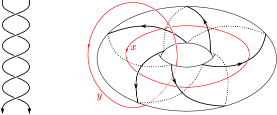
Figure 9. The braid $\sigma_{1}^{q}$ and the $(2,q)$-torus knot $T(2,q)$ ($q=5$)

$$\begin{cases}x=x_{2}(x_{2}\cdot\sigma_{1}^{-1})\cdots(x_{2}\cdot\sigma_{1}^{-(q-1)})=x_{2}(x_{1}x_{2})^{m}=g_{1}^{-1}g_{2}^{m+1},\\ y=x_{1}x_{2}=g_{2}.\end{cases}$$ (1)

Consider the non-abelian irreducible representation $\rho\colon\pi_{1}(S^{3}\setminus\hat{b})\to SL_{2}(\mathbb{C})$ given by

$$\rho(x)=\left(\begin{array}[]{cc}s&1\\ u&v\end{array}\right)\ \ \textrm{and}\ \ \rho(y)=\left(\begin{array}[]{cc}\xi_{r}&0\\ 0&\xi^{-1}_{r}\end{array}\right),$$

where $u=sv-1\neq 0$, $r$ is odd $(0<r<q)$ and $\xi_{r}=\exp\left(\displaystyle\frac{\sqrt{-1}\pi r}{q}\right)$. By the relation $x^{2}=y^{q}$, it holds that $\rho(x)^{2}=\rho(y)^{q}=-I_{2}$ and we obtain $u=-1-s^{2}$ and $v=-s$. From (1), we have

$$\rho(g_{1}) =\rho(y)^{m+1}\rho(x)^{-1}=\left(\begin{array}[]{cc}-\sqrt{-1}^{r}\xi^{\frac{1}{2}}_{r}s&-\sqrt{-1}^{r}\xi^{\frac{1}{2}}_{r}\\ \sqrt{-1}^{-r}\xi^{-\frac{1}{2}}_{r}(1+s^{2})&\sqrt{-1}^{-r}\xi^{-\frac{1}{2}}_{r}s\end{array}\right),$$

$$\rho(g_{2}) =\rho(y)=\left(\begin{array}[]{cc}\xi_{r}&0\\ 0&\xi^{-1}_{r}\end{array}\right).$$

We regard $F_{2}$ as being generated by $g_{1}$ and $g_{2}$, and then a presentation of $B_{2}\ltimes F_{2}$ is written as

$$\left\langle g_{1},g_{2},\sigma_{1}\mathrel{}\middle|\mathrel{}g_{1}\sigma_{1}=\sigma_{1}g_{2}g_{1}^{-1},g_{2}\sigma_{1}=\sigma_{1}g_{2}\right\rangle.$$

If we set

$$\rho(\sigma_{1}):=\left(\begin{array}[]{cc}\sqrt{-1}\xi^{-\frac{1}{2}}_{r}&0\\ 0&-\sqrt{-1}\xi^{\frac{1}{2}}_{r}\end{array}\right),$$

this representation is extended to $B_{2}\ltimes F_{2}$. Since $g_{1}\cdot b=g_{2}^{m+1}g_{1}^{-1}g_{2}^{-m}$, we have

$$\frac{\partial(g_{1}\cdot b)}{\partial g_{1}}=-g_{2}^{m+1}g_{1}^{-1},$$

and thus

$$\widetilde{\mathcal{LM}}_{\mathfrak{t}_{c}}(\rho)(b) =-\rho(\sigma_{1}^{q})\rho(g_{2}^{m+1}g_{1}^{-1})t^{2m+1}$$

$$=-\left(\begin{array}[]{cc}\sqrt{-1}^{q-r}&0\\ 0&-\sqrt{-1}^{q+r}\\ \end{array}\right)\left(\begin{array}[]{cc}s&-\xi_{r}\\ \xi^{-1}_{r}(1+s^{2})&-s\end{array}\right)t^{2m+1}$$

$$=\left(\begin{array}[]{cc}-\sqrt{-1}^{q-r}st^{2m+1}&\sqrt{-1}^{q-r}\xi_{r}t^{2m+1}\\ \sqrt{-1}^{q+r}\xi^{-1}_{r}(1+s^{2})t^{2m+1}&-\sqrt{-1}^{q+r}st^{2m+1}\end{array}\right).$$

Therefore

$$\det\left(\widetilde{\mathcal{LM}}_{\mathfrak{t}_{c}}(\rho)(b)-\rho(b)\right) =\det\left(\begin{array}[]{cc}-\sqrt{-1}^{q-r}(1+st^{2m+1})&\sqrt{-1}^{q-r}\xi_{r}t^{2m+1}\\ \sqrt{-1}^{q+r}\xi^{-1}_{r}(1+s^{2})t^{2m+1}&\sqrt{-1}^{q+r}(1-st^{2m+1})\end{array}\right)$$

$$=-\sqrt{-1}^{2q}-\sqrt{-1}^{2q}t^{2m+4}=1+t^{2q}$$

and

$$\det\left(\rho(x_{1}x_{2})t^{2}-I_{2}\right)=\det\left(\begin{array}[]{cc}-1+\xi_{r}t^{2}&0\\ 0&-1+\xi^{-1}_{r}t^{2}\\ \end{array}\right)=\left(1-\xi_{r}t^{2}\right)\left(1-\xi^{-1}_{r}t^{2}\right).$$

Hence

$$\Delta_{\hat{b},\rho}(t)=\frac{1+t^{2q}}{\left(1-\xi_{r}t^{2}\right)\left(1-\xi^{-1}_{r}t^{2}\right)}$$

and this is a Laurent polynomial in $\mathbb{C}[t^{\pm 1}]$, justifying the result that the twisted Alexander invariant associated with a non-abelian $SL_{2}(\mathbb{C})$-representation is a Laurent polynomial by Kitano and Morifuji [9, Theorem 3.1].

References

- [1] Paolo Bellingeri and Arthur Soulié. A note on representations of welded braid groups. J. Knot Theory Ramifications, 29(12):2050082, 21, 2020.
- [2] Stephen Bigelow and Jianjun Paul Tian. Generalized Long-Moody representations of braid groups. Commun. Contemp. Math., 10(suppl. 1):1093–1102, 2008.
- [3] J. S. Birman. Braids, links, and mapping class groups. Annals of Mathematics Studies, No. 82. Princeton University Press, Princeton, N.J.; University of Tokyo Press, Tokyo, 1974.
- [4] Ȧke Björck and Sven Hammarling. A Schur method for the square root of a matrix. Linear Algebra Appl., 52/53:127–140, 1983.
- [5] Werner Burau. Über Zopfgruppen und gleichsinnig verdrillte Verkettungen. Abh. Math. Sem. Univ. Hamburg, 11(1):179–186, 1935.
- [6] Anthony Conway. Burau maps and twisted Alexander polynomials. Proc. Edinb. Math. Soc. (2), 61(2):479–497, 2018.
- [7] G. W. Cross and P. Lancaster. Square roots of complex matrices. Linear and Multilinear Algebra, 1:289–293, 1973/74.
- [8] Christian Kassel and Vladimir Turaev. Braid groups, volume 247 of Graduate Texts in Mathematics. Springer, New York, 2008. With the graphical assistance of Olivier Dodane.
- [9] Teruaki Kitano and Takayuki Morifuji. Divisibility of twisted Alexander polynomials and fibered knots. Ann. Sc. Norm. Super. Pisa Cl. Sci. (5), 4(1):179–186, 2005.
- [10] Teruaki Kitano and Takayuki Morifuji. Twisted Alexander polynomials for irreducible -representations of torus knots. Ann. Sc. Norm. Super. Pisa Cl. Sci. (5), 11(2):395–406, 2012.
- [11] Xiao Song Lin. Representations of knot groups and twisted Alexander polynomials. Acta Math. Sin. (Engl. Ser.), 17(3):361–380, 2001.
- [12] D. D. Long. Constructing representations of braid groups. Comm. Anal. Geom., 2(2):217–238, 1994.
- [13] Arthur Soulié. The Long-Moody construction and polynomial functors. Ann. Inst. Fourier (Grenoble), 69(4):1799–1856, 2019.
- [14] Arthur Soulié. Generalized Long–Moody functors. Algebr. Geom. Topol., 22(4):1713–1788, 2022.
- [15] Masaaki Wada. Twisted Alexander polynomial for finitely presentable groups. Topology, 33(2):241–256, 1994.