Federated Dynamic Neural Network for Deep MIMO Detection

Abstract

In this paper, we develop a dynamic detection network (DDNet) based detector for multiple-input multiple-output (MIMO) systems. By constructing an improved DetNet (IDetNet) detector and the OAMPNet detector as two independent network branches, the DDNet detector performs sample-wise dynamic routing to adaptively select a better one between the IDetNet and the OAMPNet detectors for every samples under different system conditions. To avoid the prohibitive transmission overhead of dataset collection in centralized learning (CL), we propose the federated averaging (FedAve)-DDNet detector, where all raw data are kept at local clients and only locally trained model parameters are transmitted to the central server for aggregation. To further reduce the transmission overhead, we develop the federated gradient sparsification (FedGS)-DDNet detector by randomly sampling gradients with elaborately calculated probability when uploading gradients to the central server. Based on simulation results, the proposed DDNet detector consistently outperforms other detectors under all system conditions thanks to the sample-wise dynamic routing. Moreover, the federated DDNet detectors, especially the FedGS-DDNet detector, can reduce the transmission overhead by at least 25.7% while maintaining satisfactory detection accuracy.

I Introduction

Multiple-input multiple-output (MIMO) technique has been widely applied to various wireless communication systems for its high spectrum efficiency and link reliability [1, 2]. To embrace these benefits, efficient signal detection algorithms are critical to the receiver design [3]. Over the last decades, various detectors with different complexities have been proposed, among which the maximum likehood (ML) detector can obtain the best accuracy by exhaustively searching the possible signal space. However, the overwhelming complexity of the ML detector makes it nearly impractical in real systems. Sphere decoding (SD) algorithm [4] limits the searching space and can achieve near-optimal performance. Other detectors that offer relatively desired performance with lower complexity include the approximate message passing (AMP) detector [5] and the semidefinite relaxation (SDR) detector [6]. The AMP detector is derived from a strict approximation of Gaussian belief propagation and performs well on independent identically distributed (i.i.d.) Gaussian channels. The SDR detector formulates the MIMO detection problem as a non-convex homogeneous quadratically constrained quadratic problem and exhibits strong robustness. Besides, the linear minimum-mean-squared-error (LMMSE) detector provides acceptable performance with lower accuracy and is widely adopted in practical systems [7].

Motivated by the successful applications of deep learning (DL) in physical layer communications [8, 9, 10, 11, 12, 13, 14, 15, 16], many recent works resort to DL, especially deep unfolding for the MIMO detection problem [17, 18, 19, 20, 21, 22, 23]. In deep unfolding, trainable weights and non-linearities are added to each iteration of the detection, and are then optimized to improve the performance. For example,the DetNet detector [17] unfolds a projected gradient descent algorithm, which can achieve better accuracy than the SDR detector in most cases. By unfolding the orthogonal AMP (OAMP) algorithm and adding only several trainable parameters per layer, the OAMPNet detector [18] exhibits promising advantages over the conventional OAMP algorithm. Despite various deep unfolding-based detectors were subsequently proposed [20, 21, 22, 23], there is no single detector that can achieve the optimal accuracy with acceptable complexity under all different system setups and channel conditions.

Recently, dynamic neural networks have attracted growing attention for its remarkable advantages in terms of adaptiveness, accuracy, and computational efficiency [24, 25, 26]. Most prevalent DL algorithms [27, 28, 29, 30, 31, 32, 33, 34] adopt static models, where both the computational structures and the network parameters are fixed in the testing stage, i.e., every testing input goes through the same mathematical operations, which may limit the representation power and the efficiency of the DL models [25]. In contrast, dynamic neural networks adapt their structures or parameters to different inputs by selectively activating model components, e.g., layers or subnetworks, according to different inputs. For instance, for the switch transformer structure in [26], multiple network branches are built in parallel and are selectively executed based on the prediction of a front routing layers. In particular, only the $K$ network branches corresponding to the top-$K$ elements of the routing vector would be activated by the front routing layers, and an auxiliary loss is adopted to encourage these network branches to be activated with a balanced probability. The dynamic structure proposed in [26] illuminates a potential solution to MIMO detection under varying system conditions. More specifically, we can build different detectors as independent network branches and design a routing module to adaptively select an optimal detector conditioned on the input samples that contain the information of the system conditions.

On the other hand, most DL based works for physical layer communications are based on centralized learning (CL), where the networks are trained in the central server with the training data collected from the clients. However, the transmission of the whole training dataset from the clients to the central server results in prohibitive transmission overhead and poses a threat to data privacy. To tackle these problems, decentralized learning becomes a natural solution, where all the raw data are kept at clients and only locally trained model parameters are transmitted to the central server [35, 36, 37, 38]. Another underlying motivation is that the local training enables decentralized learning algorithms to handle the real-time changes lying in local datasets, which is a competitive advantage for latency sensitive applications like MIMO detection in dynamic wireless communication environments [35]. As an emerging branch of decentralized learning, federated learning (FL) distinguishes from other decentralized learning approaches in that it can deal with non-i.i.d. and unbalanced local datasets [37, 36, 38]. There are already some works that leverage FL for wireless communication applications [39], such as channel estimation [40], hybrid beamforming [41], and intelligent reflecting surface (IRS) achievable rate optimization [42], etc. In particular, FL based channel estimation algorithms have been developed in [40] for both conventional and IRS assisted massive MIMO systems, which obtain satisfactory performance closed to CL but require much lower transmission overhead. In [41], a FL based hybrid beamforming scheme has been proposed for mmwave massive MIMO systems. Notice that in both [40] and [41], the clients only conduct one time stochastic gradient descent and then upload the gradients to the central server during every epoch, which is sometimes inefficient [43]. To enhance the training efficiency, a federated averaging (FedAve) algorithm in [36] has been developed, where clients execute multiple local parameter updates before uploading the network weights to the central server. The work in [44] has provided the theoretical analysis of FedAve algorithm and proved its convergence on both i.i.d. and non-i.i.d. data with decaying learning rate. To further reduce the transmission overhead, [45] and [46] drop out small gradients when transmitting locally trained gradients to the central server.

To improve the detection accuracy, reduce the transmission overhead, and protect the data privacy, we develop the federated dynamic detection network (DDNet) based detectors for MIMO systems by borrowing ideas from dynamic neural networks and FL. The main contributions of this work can be summarized as following:

• To enhance the overall detection accuracy under varying system conditions, we design the architecture of the DDNet detector, where an improved DetNet (IDetNet) detector and the OAMPNet detector are built as two independent network branches. Moreover, a specially designed route network (RouteNet) performs sample-wise dynamic routing among the IDetNet and the OAMPNet detectors, i.e., adaptively selecting a better detector for every sample under different system conditions. To the best of authors’ knowledge, this is the first work that introduces dynamic neural networks into wireless communications.

• To reduce the transmission overhead and protect the data privacy, we propose the FedAve-DDNet detector, where OAMPNet is trained in CL way by the clients for its low training cost, while IDetNet and RouteNet are successively trained by the FedAve algorithm.

• To further reduce the transmission overhead, we develop the federated gradient sparsification (FedGS)-DDNet detector by randomly discarding gradients with elaborately calculated probability while uploading local gradients to the central server. The gradient sparsification technique only involves addition, multiplication, and minimization operations, and therefore is computationally efficient.

The rest of this paper is organized as follows. The MIMO detection problem is formulated in Section II. The architecture of the DDNet detector is presented in Section III. The FedAve-DDNet and the FedGS-DDNet detectors are developed in Section IV. Numerical results are provided in Section V, and main conclusions are given in Section VI.

Notations: The bold and lowercase letters denote vectors while the bold and capital letters denote matrices; $[\bm{z}]_{p}$ and $\textrm{len}(\bm{z})$ denote the $p$-th entry and the length of the vector $\bm{z}$, respectively; $\Re[\cdot]$ and $\Im[\cdot]$, respectively, denote the real and the imaginary parts of matrices, vectors, or scales; $\left\|{\bm{x}}\right\|_{1}$ and $\left\|{\bm{x}}\right\|_{2}$ respectively denote the $L_{1}$ and the $L_{2}$ norms of $\bm{x}$; $|\mathbb{D}|$ denote the number of elements in the dataset $\mathbb{D}$; $(\cdot)^{T}$ denotes the transpose of a matrix or a vector; $\textrm{tr}(\cdot)$ and $\textrm{vec}(\cdot)$ denote the trace and the vectorization of a matrix, respectively; ${\mathbb{C}^{m\times n}}$ represents the $m\times n$ complex vector space; $\circ$ represents the composite mapping operation; $\mathcal{N}_{C}(\bm{0,I})$ and $\mathcal{N}(\bm{0,I})$ respectively represent the standard complex and real Gaussian distributions; $E[\cdot]$ represents the expectation with respect to all random variables within the brackets; $\leftarrow$ represents the assignment operation.

II Problem Formulation

We consider a general MIMO system as the following:

$$\tilde{\bm{y}}=\tilde{\bm{H}}\tilde{\bm{x}}+\tilde{\bm{n}},$$ (1)

where $\tilde{\bm{y}}\in\mathbb{C}^{N_{r}\times 1}$ is the received signal vector, $\tilde{\bm{H}}\in\mathbb{C}^{N_{r}\times N_{t}}$ is the channel matrix, $\tilde{\bm{x}}$ is the transmitted symbol vector drawn from the constellation alphabet $\mathbb{A}$, and $\tilde{\bm{n}}\in\mathcal{N}_{C}({0,\sigma_{n}^{2}\bm{I}})$ is the Gaussian noise with variance $\sigma_{n}^{2}$. We transform Eq. (1) into the real domain as ${\bm{y}}={\bm{H}}{\bm{x}}+{\bm{n}},$ where ${\bm{y}}=[\Re[\bm{y}],\Im[\bm{y}]]^{T}$, ${\bm{x}}=[\Re[\bm{x}],\Im[\bm{x}]]^{T}$, ${\bm{n}}=[\Re[\bm{n}],\Im[\bm{n}]]^{T}$, and

$$\bm{H}\triangleq\left[\begin{array}[]{cc}\Re(\tilde{\bm{H}})&-\Im(\tilde{\bm{H}})\\ \Im(\tilde{\bm{H}})&\Re(\tilde{\bm{H}})\end{array}\right].$$ (2)

The aim of detection algorithms is to recover the transmitted signal vector ${\bm{x}}$ from the received signal vector ${\bm{y}}$ given a known channel matrix $\bm{H}$ at the receiver. The LMMSE detector [7] is one of the most widely adopted ones and can be expressed as

$$\hat{\bm{x}}_{\textrm{LMMSE}}=\mathcal{Q}\left[\left(\bm{H}^{T}\bm{H}+\sigma_{n}^{2}\bm{I}\right)^{-1}\bm{H}^{T}\bm{y}\right],$$ (3)

where $\mathcal{Q}[\cdot]$ is the quantizer associated with the constellation alphabet $\mathbb{A}$.

III Dynamic Detection Network

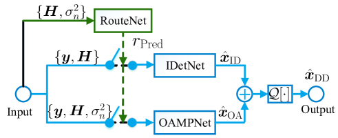
Figure 1: The structure of DDNet.

As illustrated in Fig. 1, the proposed DDNet consists of three subnetworks, i.e., IDetNet, OAMPNet and the routing module RouteNet. Note that IDetNet and OAMPNet, i.e., two different detectors, are built as two parallel network branches that are conditionally executed based on the predictions of RouteNet. The output of DDNet can be written as

$$\hat{\bm{x}}_{\textrm{DD}}=\mathcal{Q}[(1-r_{\textrm{Pred}})\hat{\bm{x}}_{\textrm{ID}}+r_{\textrm{Pred}}\hat{\bm{x}}_{\textrm{OA}}],$$ (4)

where $r_{\textrm{Pred}}\in\{0,1\}$ is the route index predicted by RouteNet, $\hat{\bm{x}}_{\textrm{ID}}$ is the estimate of IDetNet, and $\hat{\bm{x}}_{\textrm{OA}}$ is the estimate of OAMPNet. As indicated by Eq. (4), only one of IDetNet and OAMPNet would be activated by RouteNet for each sample. When the detection accuracies of IDetNet and OAMPNet for one sample are different, RouteNet would select the detector with higher accuracy. Otherwise, RouteNet would select the detector with lower complexity.

In the following, we will provide detailed descriptions of the three subnetworks, followed by detailed CL training steps and the complexity analysis.

III-A IDetNet

The structure of IDetNet is enlightened by [17]. Each layer of IDetNet mimics one iteration of the projected gradient descent optimization, and the $k$-th layer can be mathematically expressed as

$$\bm{z}_{k}\!\! = \!\!{\mathcal{F}}_{\mathrm{Relu}}({\mathcal{F}}_{\mathrm{Den}}^{k,1}([\bm{v}_{k},\bm{H}^{T}\bm{y},\bm{H}^{T}\bm{H}\hat{\bm{x}}_{k},\hat{\bm{x}}_{k}])),$$ (5a)

$${\bm{v}}_{k+1}\!\! = \!\!\mathcal{F}_{\mathrm{Smo}}^{k,1}({\mathcal{F}}_{\mathrm{Den}}^{k,2}(\bm{z}_{k}),{\bm{v}}_{k}),$$ (5b)

$$\hat{\bm{x}}_{k+1}\!\! = \!\!\mathcal{F}_{\mathrm{Smo}}^{k,2}({\mathcal{F}}_{\mathrm{Lss}}^{k}({\mathcal{F}}_{\mathrm{Den}}^{k,3}(\bm{z}_{k})),\hat{\bm{x}}_{k}),$$ (5c)

where both $\bm{z}_{k}$ and $\bm{v}_{k}$ are intermediate iteration variables, ${\mathcal{F}}_{\mathrm{Relu}}(\bm{s})=\max\{\bm{s},0\}$ is the nonlinear activation function, and

$${\mathcal{F}}_{\mathrm{Lss}}^{k}(\bm{s};\beta_{k})=-1+\frac{{\mathcal{F}}_{\mathrm{Relu}}(\bm{s}+\beta_{k})}{|\beta_{k}|}-\frac{{\mathcal{F}}_{\mathrm{Relu}}(\bm{s}-\beta_{k})}{|\beta_{k}|}$$ (6)

is the element-wise linear soft sign function with $\beta_{k}$ being a trainable parameter. Besides, the $i$-th dense layer in the $k$-th layer of IDetNet can be expressed as

$$\mathcal{F}_{\mathrm{Den}}^{k,i}(\bm{s};\bm{w}_{k,i},\bm{b}_{k,i})=\bm{w}_{k,i}\bm{s}+\bm{b}_{k,i},\quad i=1,2,3,$$ (7)

where $\bm{w}_{k,i}$ and $\bm{b}_{k,i}$ are respectively the weight and the bias of the dense layer. Moreover, we adopt the following smoothing function

$$\mathcal{F}_{\mathrm{Smo}}^{k,i}(\bm{s}_{{k+1}},\bm{s}_{{k}},\alpha_{k,i})=(1-\alpha_{k,i})\bm{s}_{{k+1}}+\alpha_{k,i}\bm{s}_{{k}},\ i=1,2,$$ (8)

where $\alpha_{k,i}$ is the trainable smoothing factor. Denote $K_{\textrm{ID}}$ as the layer number of IDetNet. By cascading $K_{\textrm{ID}}$ layers, we can obtain the output of IDetNet as

$$\hat{\bm{x}}_{\textrm{ID}}\buildrel\Delta\over{=}\hat{\bm{x}}_{K_{\textrm{ID}}+1}\buildrel\Delta\over{=}\mathcal{F}_{\mathrm{IDetNet}}(\bm{H},\bm{y};\bm{\Omega}_{\mathrm{ID}}),$$ (9)

where $\bm{\Omega}_{\mathrm{ID}}\buildrel\Delta\over{=}\{\beta_{k},\{\bm{w}_{k,i},\bm{b}_{k,i}\}_{i=1,2,3},\{\alpha_{k,i}\}_{i=1,2}\}_{k=1}^{K_{\textrm{ID}}}$ is the trainable parameter of IDetNet to be optimized. The loss function of IDetNet can be written as

$$\mathcal{L}_{\textrm{ID}}\left(\bm{\Omega}_{\mathrm{ID}}\right)=\frac{1}{{D}}\sum\limits_{d=1}^{D}\sum\limits_{k=2}^{K_{\textrm{ID}}+1}\|\hat{\bm{x}}_{k}^{(d)}-\bm{x}^{(d)}\|_{2}^{2},$$ (10)

where $D$ is the batch size, and $d$ denotes the index of the training samples.

Compared with DetNet in [17], we make two improvements in IDetNet:

1. We set $\{\beta_{k}\}_{k=1}^{K_{\textrm{ID}}}$ to be trainable parameters, which allows each layer of IDetNet to have a linear soft sign function with different softness. As indicated in Eq. (6), the function ${\mathcal{F}}_{\mathrm{Lss}}^{k}$ with a smaller $\beta_{k}$ has a larger slope near the zero point and thus makes a harder decision about the input $\bm{s}$, which results in faster convergence but may potentially increase the accumulated estimated error of the subsequent layers. In IDetNet, layers at different depths are able to learn proper $\{\beta_{k}\}_{k=1}^{K_{\textrm{ID}}}$ to improve the convergence speed and achieve better performance.

2. We exploit smoothing function $\mathcal{F}_{\mathrm{Smo}}^{k,i}$ for the updates of $\hat{\bm{x}}_{k}$ and $\bm{v}_{k}$. The smoothing factor, $\alpha_{k,i}$, is a trainable parameters, and allows each layer of IDetNet to assign different weights to the outputs of the prior layer. The smoothing function can improve the stability and accuracy of the network.

III-B OAMPNet

OAMPNet, originally proposed in [18], will be briefly illustrated here. The $k$-th layer of OAMPNet can be described as following:

$$v_{k}^{2} =\frac{\|\bm{y}-\bm{H}\hat{\bm{x}}_{k}\|_{2}^{2}-\textrm{tr}(\bm{R}_{\bm{n}})}{\textrm{tr}(\bm{H}^{T}\bm{H})},$$ (11a)

$$\bm{A}_{k} =\frac{2N_{t}v_{k}^{2}\bm{H}^{T}(v_{k}^{2}\bm{HH}^{T}+\bm{R}_{\bm{n}})^{-1}}{\textrm{tr}(v_{k}^{2}\bm{H}^{T}(v_{k}^{2}\bm{HH}^{T}+\bm{R}_{\bm{n}})^{-1}\bm{H})},$$ (11b)

$$\bm{z}_{k} =\hat{\bm{x}}_{k}+\gamma_{k,1}\bm{A}_{k}(\bm{y}-\bm{H}\hat{\bm{x}}_{k}),$$ (11c)

$$\bm{C}_{k} =\bm{I}-\gamma_{k,2}\bm{A}_{k}\bm{H},$$ (11d)

$$\tau_{k}^{2} =\frac{{\textrm{tr}(\bm{C}_{k}\bm{C}_{k}^{T})}v_{k}^{2}+{\textrm{tr}(\bm{A}_{k}\bm{R}_{\bm{n}}\bm{A}_{k}^{T})}}{2N_{t}},$$ (11e)

$$\hat{\bm{x}}_{k+1} =\eta_{k}\left(\bm{z}_{k},\tau_{k}^{2};\gamma_{k,3},\gamma_{k,4}\right),$$ (11f)

where $\bm{R}_{\bm{n}}=\sigma_{n}^{2}\bm{I}$ is the covariance matrix of the noise $\bm{n}$, $v_{k}^{2}$ and $\tau_{k}^{2}$ are error estimators, $\bm{A}_{k}$ is the de-correlated matrix, $\bm{z}_{k}$ is the linear estimator, and $\bm{C}_{k}$ is an intermediate iteration variable. Moreover, $\eta_{k}(\cdot)$ is the nonlinear estimator, expressed as

$$\eta_{k}\left(\bm{z}_{k},\tau_{k}^{2};\gamma_{k,3},\gamma_{k,4}\right)\!=\!\gamma_{k,3}\left({E}\left\{\bm{x}|\bm{z}_{k},\tau_{k}^{2}\right\}-\gamma_{k,4}\bm{z}_{k}\right),$$ (12)

where ${E}\left\{\bm{x}|\bm{z}_{k},\tau_{k}^{2}\right\}$ is the MMSE estimator of $\bm{x}$. Denote $K_{\textrm{OA}}$ as the number of layers in OAMPNet. The output of OAMPNet can be expressed as

$$\hat{\bm{x}}_{\textrm{OA}}\buildrel\Delta\over{=}\hat{\bm{x}}_{K_{\textrm{OA}}+1}\buildrel\Delta\over{=}\mathcal{F}_{\mathrm{OAMPNet}}(\bm{H},\bm{y},\sigma_{n}^{2};\bm{\Omega}_{\mathrm{OA}}),$$ (13)

where $\bm{\Omega}_{\mathrm{OA}}\buildrel\Delta\over{=}\{\gamma_{i,k}\}_{i,k=1}^{4,K_{\textrm{OA}}}$ is the trainable parameter set of OAMPNet to be optimized. The loss function of OAMPNet is

$$\mathcal{L}_{\textrm{OA}}\left(\bm{\Omega}_{\mathrm{OA}}\right)=\frac{1}{{D}}\sum\limits_{d=1}^{D}\sum\limits_{k=2}^{K_{\textrm{OA}}+1}\|\hat{\bm{x}}_{k}^{(d)}-\bm{x}^{(d)}\|_{2}^{2}.$$ (14)

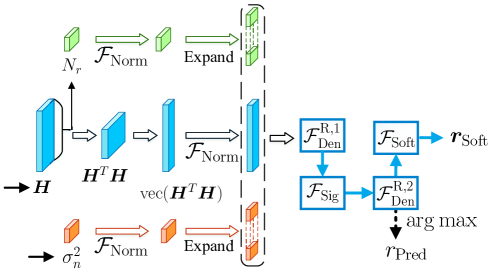
Figure 2: The structure of RouteNet.

III-C RouteNet

The goal of RouteNet is to perform sample-wise dynamic routing between IDetNet and OAMPNet, i.e., adaptively selecting a better subnetwork for each sample according to the system conditions, including the signal-to-noise ratio (SNR), the number of received antennas, and the channel statistics. Therefore, we set the noise power $\sigma_{n}^{2}$, the number of received antennas $N_{r}$, and the channel matrix $\bm{H}$ as the input data to instruct RouteNet in subnetwork routing under different system conditions. As shown in Fig. 2, we first infer the value of $N_{r}$ from the shape of $\bm{H}$ for each sample, and then adopt $\bm{H}^{T}\bm{H}$ rather than $\bm{H}$ as an input to avoid the varying dimensionality of $\bm{H}$ in input samples. Moreover, we normalize $\sigma_{n}^{2}$, $N_{r}$, and $\bm{H}$ to a unified interval by a linear transformation,

$${\mathcal{F}}_{\mathrm{Norm}}(\bm{s};\bm{s}_{\textrm{max}},\bm{s}_{\textrm{min}})=(\bm{s}-\bm{s}_{\textrm{min}})/(\bm{s}_{\textrm{max}}-\bm{s}_{\textrm{min}}),$$ (15)

where $\bm{s}_{\textrm{max}}\!=\!\max_{\bm{s}\in\mathbb{D}}\bm{s}$ and $\bm{s}_{\textrm{min}}\!=\!\min_{\bm{s}\in\mathbb{D}}\bm{s}$ are respectively the element-wise maximum and minimum vectors over datasets $\mathbb{D}$. Next, we expand both ${\mathcal{F}}_{\mathrm{Norm}}(\sigma_{n}^{2})$ and ${\mathcal{F}}_{\mathrm{Norm}}(N_{r})$ to vectors of length $N_{t}$. The reason that we conduct the dimension expansion is to prevent ${\mathcal{F}}_{\mathrm{Norm}}(\sigma_{n}^{2})$ and ${\mathcal{F}}_{\mathrm{Norm}}(N_{r})$ from being ignored by RouteNet due to their extremely small dimensions. It is also reasonable to expand $\sigma_{n}^{2}$ and $N_{r}$ to vectors of other proper lengths.

As shown in Fig. 2, the input vector of RouteNet can be written as

$$\bm{s}_{\textrm{RO}}=[{\mathcal{F}}_{\mathrm{Norm}}(\sigma_{n}^{2})\bm{1}_{N_{t}},{\mathcal{F}}_{\mathrm{Norm}}\textrm{vec}(\bm{H}^{T}\bm{H}),{\mathcal{F}}_{\mathrm{Norm}}(N_{r})\bm{1}_{N_{t}}].$$ (16)

Since RouteNet only consists of two dense layers, i.e., $\{\mathcal{F}_{\mathrm{Den}}^{\textrm{R},i}\}_{i=1,2}$, we adopt the Sigmoid function, $\mathcal{F}_{\mathrm{Sig}}(\bm{s})=1/(1+e^{-\bm{s}})$, instead of the ReLU function to improve the nonlinear fitting capability of RouteNet. We add the softmax function, $\mathcal{F}_{\mathrm{Soft}}$, to the output layer, which is given by

$$\left[\mathcal{F}_{\mathrm{Soft}}(\bm{s})\right]_{p}=\frac{e^{\left[\bm{s}\right]_{p}}}{\sum_{p=1}^{p=\textrm{len}(\bm{s})}e^{\left[\bm{s}\right]_{p}}},\ p=1,2,\cdots,\textrm{len}(\bm{s}).$$ (17)

The route index $r_{\textrm{Pred}}\in\{0,1\}$ can be obtained by

$$r_{\textrm{Pred}}=\arg\max\{\mathcal{F}_{\mathrm{Den}}^{\textrm{R},2}\circ{\mathcal{F}}_{\mathrm{Sig}}\circ\mathcal{F}_{\mathrm{Den}}^{\textrm{R},1}(\bm{s}_{\textrm{RO}})\}-1.$$ (18)

Define the bit error function as

$${\mathcal{F}}_{\mathrm{BE}}(\hat{\bm{x}};\bm{x})={\|\mathcal{Q}[\bm{x}]-\mathcal{Q}[\hat{\bm{x}}]\|_{1}},$$ (19)

where $\bm{x}$ and $\hat{\bm{x}}$ respectively denote the transmitted signal and the estimated signal. The route label $\bm{r}_{\textrm{Lab}}$ is obtained by measuring the bit errors of OAMPNet and IDetNet, and can be written as

$$\begin{array}[]{l}\bm{r}_{\textrm{Lab}}=\left\{\begin{array}[]{ll}$[1,0]$,&\textrm{if }{\mathcal{F}}_{\mathrm{BE}}(\hat{\bm{x}}_{\textrm{ID}})\leq{\mathcal{F}}_{\mathrm{BE}}(\hat{\bm{x}}_{\textrm{OA}});\\ $[0,1]$,&\mathrm{otherwise}.\end{array}\right.\end{array}$$ (23)

In the case of ${\mathcal{F}}_{\mathrm{BE}}(\hat{\bm{x}}_{\textrm{ID}})={\mathcal{F}}_{\mathrm{BE}}(\hat{\bm{x}}_{\textrm{OA}})$, IDetNet would be selected for its lower complexity compared with OAMPNet. The classification error in the case of ${\mathcal{F}}_{\mathrm{BE}}(\hat{\bm{x}}_{\textrm{ID}})={\mathcal{F}}_{\mathrm{BE}}(\hat{\bm{x}}_{\textrm{OA}})$ would increase the computational cost while the classification error in the case of ${\mathcal{F}}_{\mathrm{BE}}(\hat{\bm{x}}_{\textrm{ID}})\neq{\mathcal{F}}_{\mathrm{BE}}(\hat{\bm{x}}_{\textrm{OA}})$ would increase the bit errors. The loss function can be written as

$$\mathcal{L}_{\textrm{RO}}\left(\bm{\Omega}_{\textrm{RO}}\right)=\frac{1}{{D}}\sum\limits_{d=1}^{D}\left(entropy(\bm{r}_{\textrm{Lab}}^{(d)},\bm{r}_{\textrm{Soft}}^{(d)})+\xi({\mathcal{F}}_{\mathrm{BE}}(\hat{\bm{x}}_{\textrm{DD}}^{(d)})-\min\{{\mathcal{F}}_{\mathrm{BE}}(\hat{\bm{x}}_{\textrm{ID}}^{(d)}),{\mathcal{F}}_{\mathrm{BE}}(\hat{\bm{x}}_{\textrm{OA}}^{(d)})\})\right),$$ (24)

where $entropy(\bm{r}_{\textrm{Lab}}^{(d)},\bm{r}_{\textrm{Soft}}^{(d)})=\sum\nolimits_{p=1}^{\textrm{len}(\bm{r}_{\textrm{Soft}})}\left[\bm{r}_{\textrm{Lab}}^{(d)}\right]_{p}\log\left[\bm{r}_{\textrm{Soft}}^{(d)}\right]_{p}$ is the categorical cross entropy, $\bm{\Omega}_{\textrm{RO}}\buildrel\Delta\over{=}\{\bm{w}_{\textrm{R},i},\bm{b}_{\textrm{R},i}\}_{i=1,2}$ is the trainable parameter of RouteNet, $\bm{r}_{\textrm{Soft}}={\mathcal{F}}_{\mathrm{Soft}}\circ\mathcal{F}_{\mathrm{Den}}^{\textrm{R},2}\circ{\mathcal{F}}_{\mathrm{Sig}}\circ\mathcal{F}_{\mathrm{Den}}^{\textrm{R},1}(\bm{s}_{\textrm{RO}})$ is the output of RouteNet, and $\xi>0$ is the penalty coefficient. A larger $\xi$ indicates less tolerance to the accuracy loss of DDNet, and thus forces the algorithm to be more sensitive to the classification errors that increase the bit errors.

Remark 1: Due to the high detection accuracy of the IDetNet and the OAMPNet detectors in high SNR regions, most samples would be detected by the IDetNet or the OAMPNet detectors without errors. In this case, the number of samples with the route label $\bm{r}_{\textrm{Lab}}=[1,0]$ would be significantly more than those with the route label $\bm{r}_{\textrm{Lab}}=[0,1]$. Such an unbalanced route dataset would result in low classification accuracy. Therefore, before we randomly shuffle the samples under varying SNRs, we remove extra samples to keep the balance of the route dataset.

Remark 2: We choose the OAMPNet and the IDetNet detectors as two network branches for their different computational complexities and varying accuracies under different system conditions. In this case, RouteNet is expected not only to select a detector with better accuracy under different system conditions, but also to select a detector with lower complexity without making any compromise on accuracy. Furthermore, RouteNet can be easily extended to the route of multiple parallel detectors by generalizing the binary classification label Eq. (23) into a multi-classification label. Moreover, conventional detectors could also serve as branches. By adding one more detector with lower complexity as a branch, the complexity of the whole network would be reduced. By adding one more detector with better accuracy as a branch, the accuracy of the whole network would be improve. For example, we could build the LMMSE, the IDetNet, the OAMPNet and the SD detectors as four parallel branches. Then, by properly designing the route label and the loss function, we could train a route network to select the detector with the lowest complexity among those exhibiting the same optimal accuracy. Due to the lack of space, the extension to multiple parallel detectors would be left as future work.

Remark 3: Since various detectors may have different complexities and exhibit different accuracies, we can balance the accuracy and the complexity by assigning route labels according to certain rules. For instance, we can define the route label, $\bm{r}^{\prime}_{\textrm{Lab}}$, as

$$\begin{array}[]{l}\bm{r}^{\prime}_{\textrm{Lab}}=\left\{\begin{array}[]{ll}$[1,0]$,&{\mathcal{F}}_{\mathrm{BE}}(\hat{\bm{x}}_{\textrm{D1}})-{\mathcal{F}}_{\mathrm{BE}}(\hat{\bm{x}}_{\textrm{D2}})\leq\epsilon;\\ $[0,1]$,&\textrm{otherwise},\end{array}\right.\end{array}$$ (28)

where $\hat{\bm{x}}_{\textrm{D1}}$ and $\hat{\bm{x}}_{\textrm{D2}}$ are respectively the estimates of Detector-1 and Detector-2. If the complexity of Detector-1 is higher than Detector-2, then we can select a proper $\epsilon<0$ such that RouteNet only uses Detector-1 when the accuracy gain of Detector-1 relative to Detector-2 reaches a certain value. Otherwise, we set $\epsilon>0$ if the complexity of Detector-1 is lower than Detector-2. The flexibility design of the route label endows the proposed DDNet with great potential in real applications.

III-D Centralized Training Steps and Complexity Analysis

Centralized training steps: In CL, the whole training dataset $\mathbb{D}_{\textrm{whole}}$ can be obtained by uploading the local datasets of all clients to the central server. Then, the training process is executed by the central server. The detail training steps of the CL-DDNet detector are given as follows:

1. Initialize $\bm{\Omega}_{\mathrm{ID}}$: $\{\beta_{k}\}_{k=1}^{K_{\textrm{ID}}}=0.7$; $\{\alpha_{k,i}\}_{i,k=1}^{2,K_{\textrm{ID}}}=0.8$; $\{\bm{w}_{k,i},\bm{b}_{k,i}\}_{i,k=1}^{3,K_{\textrm{ID}}}\in\mathcal{N}(\bm{0,0.01I})$.

2. Update $\bm{\Omega}_{\mathrm{ID}}$ by using the ADAM algorithm to minimize $\mathcal{L}_{\textrm{ID}}\left(\bm{\Omega}_{\mathrm{ID}}\right)$ until convergence, and then obtain the trained parameter: $\bm{\Omega}_{\mathrm{ID}}^{*}\leftarrow\bm{\Omega}_{\mathrm{ID}}$.

3. Initialize $\bm{\Omega}_{\mathrm{OA}}$: $\{\gamma_{i,k}\}_{i,k=1}^{3,K_{\textrm{OA}}}=1.0$; $\{\gamma_{4,k}\}_{k=1}^{K_{\textrm{OA}}}=0.0$.

4. Update $\bm{\Omega}_{\mathrm{OA}}$ by using the ADAM algorithm to minimize $\mathcal{L}_{\textrm{OA}}\left(\bm{\Omega}_{\mathrm{OA}}\right)$ until convergence, and then obtain the trained parameter: $\bm{\Omega}_{\mathrm{OA}}^{*}\leftarrow\bm{\Omega}_{\mathrm{OA}}$.

5. Obtain the route dataset $\{(\bm{H},\sigma_{n}^{2}),(\bm{r}_{\textrm{Lab}})\}$ by Eq. (23).

6. Initialize $\bm{\Omega}_{\textrm{RO}}$: $\{\bm{w}_{\textrm{R},i},\bm{b}_{\textrm{R},i}\}_{i=1,2}\in\mathcal{N}(\bm{0,0.01I})$.

7. Update $\bm{\Omega}_{\mathrm{RO}}$ by using the ADAM algorithm to minimize $\mathcal{L}_{\textrm{RO}}\left(\bm{\Omega}_{\mathrm{RO}}\right)$ until convergence, and then obtain the trained parameter: $\bm{\Omega}_{\mathrm{RO}}^{*}\leftarrow\bm{\Omega}_{\mathrm{RO}}$.

Note that Step (a) $\sim$ (b) and Step (c) $\sim$ (d) can be executed in parallel.

TABLE I: Complexity comparisons of the detectors

Detector	Computational complexity	Trainable parameters
LMMSE	$O(N_{t}^{3})$	0
OAMPNet	$O(K_{\textrm{OA}}N_{t}^{3})$	32
DetNet	$O(K_{\textrm{ID}}N_{t}^{2})$	249600
IDetNet	$O(K_{\textrm{ID}}N_{t}^{2}+K_{\textrm{ID}}N_{t})$	249720
DDNet	$O(K_{\textrm{ID}}N_{t}^{2}+K_{\textrm{ID}}N_{t}+N_{t}^{2})\sim O(K_{\textrm{OA}}N_{t}^{3})$	389401

TABLE II: Default Parameters of DDNet

Layer	$\{{\mathcal{F}}_{\mathrm{Den}}^{k,1}\}_{k=1}^{K_{\textrm{ID}}}$	$\{{\mathcal{F}}_{\mathrm{Den}}^{k,i}\}_{k,i=1,2}^{K_{\textrm{ID}},3}$	$\mathcal{F}_{\mathrm{Den}}^{\textrm{R},1}$	$\mathcal{F}_{\mathrm{Den}}^{\textrm{R},2}$
Neurons	64	32	128	2

Complexity analysis: The computational complexities of the LMMSE, the OAMPNet, the DetNet, the IDetNet and the DDNet detectors are given in Tab. I. The LMMSE detector has a complexity of $O(N_{t}^{3})$ due to the matrix inversion, but requires no training and iteration. The OAMPNet detector requires the matrix inversion operation in each layer as shown in Eq. (11b), and therefore has a complexity of $O(K_{\textrm{OA}}N_{t}^{3})$. The IDetNet detector has slightly higher order of complexity than the DetNet detector since the smoothing functions in each layer introduce the extra complexity of $O(K_{\textrm{ID}}N_{t})$. Moreover, since RouteNet introduces extra complexity of $O(N_{t}^{2})$ and only activates one of the OAMPNet and the IDetNet detectors for every sample, the computational complexity of the DDNet detector varies for different samples and ranges from $O(K_{\textrm{ID}}N_{t}^{2}+K_{\textrm{ID}}N_{t}+N_{t}^{2})\sim O(K_{\textrm{OA}}N_{t}^{3})$.

Using default parameters of the DDNet detector in Tab. II as an example, we compare the numbers of trainable parameters of the LMMSE, the OAMPNet, the DetNet, the IDetNet and the DDNet detectors in Tab. I, where the layer numbers $K_{\textrm{ID}}$ and $K_{\textrm{OA}}$ are set to be 40 and 8, respectively. As shown in Tab. I, the OAMPNet detector has much fewer trainable parameters but higher computational complexity than the IDetNet detector.

Figure 3: Federated training process of the DDNet detector, where ${\mathbb{D}}_{m}$ is the local dataset at the $m$-th client. Note that the number of selected clients $M$ does not have to be consistent during the federated training processes of IDetNet and RouteNet.

IV Federated Dynamic Detection Network

FL protects the privacy of clients by leaving the raw data to local clients and only uploading model parameters to the central server for aggregation. Since OAMPNet requires very few training samples and training epoches, we will only train OAMPNet on local clients in the CL way, while train IDetNet and RouteNet in FL way. Fig. 3 illustrates the federated training process of DDNet, where $M$ clients are randomly selected to perform local updates during each global epoch. Let $\bm{\Omega}_{\mathrm{ID}}^{t}$ and $\bm{\Omega}_{\mathrm{RO}}^{t}$ respectively represent the global network parameters of IDetNet and RouteNet at the end of the $t$-th global epoch. The federated training process of IDetNet/RouteNet includes four steps:

1. Weights Broadcast: The central server broadcasts the global network parameter ($\bm{\Omega}_{\mathrm{ID}}^{t-1}$ or $\bm{\Omega}_{\mathrm{RO}}^{t-1}$) to each local client.

2. Local update: Each selected client updates their local network parameters or only calculates the local gradients of the network parameters on their local datasets in parallel.

3. Parameter upload: Each selected client uploads their local network parameters or the local gradients to the central server.

4. Global aggregation: The central server obtains global network parameters ($\bm{\Omega}_{\mathrm{ID}}^{t}$ or $\bm{\Omega}_{\mathrm{RO}}^{t}$) based on the parameters received from the clients.

In the following, we will present the FedAve-DDNet detector in detail. To further reduce the transmission overhead, we will also propose the FedGS-DDNet detector.

IV-A The FedAve-DDNet Detector

Denote the detection samples available at the $m$-th client as ${\mathbb{D}}_{m}^{\textrm{D}}$, with ${\mathbb{D}}_{m}^{\textrm{D}}\buildrel\Delta\over{=}\{(\bm{y},\bm{H},\sigma_{n}^{2}),(\bm{x})\}$ and $|{\mathbb{D}}_{m}^{\textrm{D}}|={D}_{m}^{\textrm{D}}$. We first train IDetNet following the above Step (i) $\sim$ (iv). In Step (ii), each selected client updates their local network parameters by $\ell_{m}$ successive parameter updates. During the $t$-th global epoch, the updated local network parameter of the $m$-th client, denoted as $\bm{\Omega}_{\mathrm{ID}}^{t,m}$, can be obtained by

$$\bm{\Omega}_{\mathrm{ID}}^{t,m}\leftarrow\textrm{ADAM}^{\ell_{m}}(\bm{\Omega}_{\mathrm{ID}}^{t-1},\nabla_{\bm{\Omega}_{\mathrm{ID}}}^{{\mathbb{D}}_{m}^{\textrm{D}}}\mathcal{L}_{\textrm{ID}}),$$ (29)

where $\nabla_{\bm{\Omega}_{\mathrm{ID}}}^{{\mathbb{D}}_{m}^{\textrm{D}}}\mathcal{L}_{\textrm{ID}}$ represents the gradients of $\mathcal{L}_{\textrm{ID}}$ with respect to the network parameter $\bm{\Omega}_{\mathrm{ID}}$ on the dataset ${\mathbb{D}}_{m}^{\textrm{D}}$. Moreover, $\textrm{ADAM}^{\ell_{m}}(\bm{\Omega}_{\mathrm{ID}}^{t-1},\nabla_{\bm{\Omega}_{\mathrm{ID}}}^{{\mathbb{D}}_{m}^{\textrm{D}}}\mathcal{L}_{\textrm{ID}})$ represents $\ell_{m}$ successive parameter-updates by the ADAM algorithm [47], where $\bm{\Omega}_{\mathrm{ID}}^{t-1}$ is the initial network parameter of the first parameter-update. In Step (iii), each selected client uploads their updated local parameters, i.e., $\{\bm{\Omega}_{\mathrm{ID}}^{t,m}\}_{m\in\mathbb{M}_{\textrm{ID}}}$, to the central server, where $\mathbb{M}_{\textrm{ID}}$ represents the set of selected clients during the federated training processes of IDetNet. In Step (iv), the central server obtains global network parameters by weighted aggregation. The global network parameter $\bm{\Omega}_{\mathrm{ID}}^{t}$ is given by

$$\bm{\Omega}_{\mathrm{ID}}^{t}\leftarrow\frac{\sum_{m\in\mathbb{M}_{\textrm{ID}}}{D}_{m}^{\textrm{D}}\bm{\Omega}_{\mathrm{ID}}^{t,m}}{\sum_{m\in\mathbb{M}_{\textrm{ID}}}{D}_{m}^{\textrm{D}}}.$$ (30)

After the training of OAMPNet and IDetNet, each client can obtain the route dataset ${\mathbb{D}}_{m}^{\textrm{R}}\buildrel\Delta\over{=}\{(\bm{H},\sigma_{n}^{2}),(\bm{r}_{\textrm{Lab}})\}$ for RouteNet by Eq. (23). Then, we will train RouteNet in the similar way with IDetNet. More specifically, the weight updates in the clients and the central server can be respectively given as follows:

$$\bm{\Omega}_{\mathrm{RO}}^{t,m}\!\! \leftarrow \!\!\textrm{ADAM}^{\ell_{m}}(\bm{\Omega}_{\mathrm{RO}}^{t-1},\nabla_{\bm{\Omega}_{\mathrm{RO}}}^{{\mathbb{D}}_{m}^{\textrm{R}}}\mathcal{L}_{\textrm{RO}}),$$ (31)

$$\bm{\Omega}_{\mathrm{RO}}^{t}\!\! \leftarrow \!\!\frac{\sum_{m\in\mathbb{M}_{\textrm{RO}}}{D}_{m}^{\textrm{R}}\bm{\Omega}_{\mathrm{RO}}^{t,m}}{\sum_{m\in\mathbb{M}_{\textrm{RO}}}{D}_{m}^{\textrm{R}}},$$ (32)

where ${D}_{m}^{\textrm{R}}=|{\mathbb{D}}_{m}^{\textrm{R}}|$, $\mathbb{M}_{\textrm{RO}}$ represents the set of selected clients during the federated training processes of RouteNet, and $\bm{\Omega}_{\mathrm{RO}}^{t,m}$ is the local network parameter of RouteNet for the $m$-th client during the $t$-th global epoch.

The concrete training steps of the FedAve-DDNet detector are given in Algorithm 1, where $T_{\mathrm{F,ID}}$ and $T_{\mathrm{F,RO}}$ are respectively the numbers of global epoches required for the training of IDetNet and RouteNet. Note that the training of OAMPNet, the function LocalUpdateUpload, and the function RouteDataset are all executed by local clients. Moreover, the training of OAMPNet and the local updates of IDetNet can be executed in parallel.

Algorithm 1 The FedAve-DDNet detector

Central server executes:

1:/*Train IDetNet*/

2:Initialize $\bm{\Omega}_{\mathrm{ID}}$ following Step (a) in Section III-D

3:for $t=1,2,\cdots,T_{\mathrm{F,ID}}$ do

4:     Broadcast $\bm{\Omega}_{\mathrm{ID}}^{t-1}$ to randomly selected $M$ clients

5:     for each client $m=1$ to $M_{\mathrm{ID}}$ in parallel do

6:          LocalUpdateUpload($m,\bm{\Omega}_{\mathrm{ID}}^{t-1};\mathcal{L}_{\mathrm{ID}},\ell_{m},{\mathbb{D}}_{m}^{\textrm{D}}$)

7:     end for

8:     $\bm{\Omega}_{\mathrm{ID}}^{t}\leftarrow$ Aggregation($\{\bm{\Omega}_{\mathrm{ID}}^{t,m}\}_{m\in\mathbb{M}_{\mathrm{ID}}},\{D_{m}^{\textrm{D}}\}_{m\in\mathbb{M}_{\mathrm{ID}}}$)

9:end for

10:Broadcast $\bm{\Omega}_{\mathrm{ID}}^{T_{\mathrm{F,ID}}}$ to all clients

11:/* Train RouteNet*/

12:Initialize $\bm{\Omega}_{\mathrm{RO}}$ following Step (f) in Section III-D

13:${\mathbb{D}}_{m}^{\textrm{R}}\leftarrow$ RouteDataset($m,\bm{\Omega}_{\mathrm{ID}}^{T_{\mathrm{F,ID}}},\bm{\Omega}_{\mathrm{OA}}^{*}$)

14:for $t=1,2,\cdots,T_{\mathrm{F,RO}}$ do

15:     Broadcast $\bm{\Omega}_{\mathrm{RO}}^{t-1}$ to randomly selected $M$ clients

16:     for each client $m=1$ to $M_{\mathrm{RO}}$ in parallel do

17:          LocalUpdateUpload($m,\bm{\Omega}_{\mathrm{RO}}^{t-1};\mathcal{L}_{\mathrm{RO}},\ell_{m},{\mathbb{D}}_{m}^{\textrm{R}}$)

18:     end for

19:     $\bm{\Omega}_{\mathrm{RO}}^{t}\leftarrow$ Aggregation($\{\bm{\Omega}_{\mathrm{RO}}^{t,m}\}_{m\in\mathbb{M}_{\mathrm{RO}}},\{D_{m}^{\textrm{R}}\}_{m\in\mathbb{M}_{\mathrm{RO}}}$)

20:end for

21:Broadcast $\bm{\Omega}_{\mathrm{RO}}^{T_{\mathrm{F,RO}}}$ to all clients

def Aggregation($\{\bm{\Omega}^{t,m}\}_{m\in\mathbb{M}},\{D_{m}\}_{m\in\mathbb{M}}$)

 $\bm{\Omega}^{t}\leftarrow{\sum_{m\in\mathbb{M}}{D}_{m}\bm{\Omega}^{t,m}}/{\sum_{m\in\mathbb{M}}{D}_{m}}$

 return $\bm{\Omega}^{t}$

Clients execute:

Train OAMPNet following Step (c) $\sim$ (d) in Section III-D

def LocalUpdateUpload($m,\bm{\Omega}^{t-1},\mathcal{L},\ell_{m},\mathbb{D}_{m}$)

 $\bm{\Omega}^{t,m}\leftarrow\textrm{ADAM}^{\ell_{m}}(\bm{\Omega}^{t-1},\nabla_{\bm{\Omega}}^{\mathbb{D}_{m}}\mathcal{L})$

 Upload $\bm{\Omega}^{t,m}$ to central server

def RouteDataset($m,\bm{\Omega}_{\mathrm{ID}},\bm{\Omega}_{\mathrm{OA}}$)

 Obtain the dataset ${\mathbb{D}}_{m}^{\textrm{R}}$ with Eq. (23)

 return ${\mathbb{D}}_{m}^{\textrm{R}}$

IV-B The FedGS-DDNet Detector

Different from the FedAve-DDNet detector where the clients upload local network parameters ($\bm{\Omega}_{\mathrm{ID}}^{t,m}$ or $\bm{\Omega}_{\mathrm{RO}}^{t,m}$) to the central server, the FedGS-DDNet detector requires the clients to upload locally sparsified gradients, denoted by $\mathcal{S}(\bm{g}_{\mathrm{ID}}^{t,m})$ or $\mathcal{S}(\bm{g}_{\mathrm{RO}}^{t,m})$, to the central server. Next, the central server would update the global network parameters by one time ADAM optimization, which can be written as following:

$$\bm{\Omega}_{\mathrm{ID}}^{t}\leftarrow\textrm{ADAM}^{1}(\bm{\Omega}_{\mathrm{ID}}^{t-1},\bm{g}_{\mathrm{ID}}^{t}),$$ (33)

$$\bm{\Omega}_{\mathrm{RO}}^{t}\leftarrow\textrm{ADAM}^{1}(\bm{\Omega}_{\mathrm{RO}}^{t-1},\bm{g}_{\mathrm{RO}}^{t}),$$ (34)

where $\bm{g}_{\mathrm{ID}}^{t}$ and $\bm{g}_{\mathrm{RO}}^{t}$ are weighted gradients given by

$$\bm{g}_{\mathrm{ID}}^{t}\leftarrow\frac{\sum_{m\in\mathbb{M}_{\textrm{ID}}}{D}_{m}^{\textrm{D}}\mathcal{S}(\bm{g}_{\mathrm{ID}}^{t,m})}{\sum_{m\in\mathbb{M}_{\textrm{ID}}}{D}_{m}^{\textrm{D}}},$$ (35)

$$\bm{g}_{\mathrm{RO}}^{t}\leftarrow\frac{\sum_{m\in\mathbb{M}_{\textrm{RO}}}{D}_{m}^{\textrm{R}}\mathcal{S}(\bm{g}_{\mathrm{RO}}^{t,m})}{\sum_{m\in\mathbb{M}_{\textrm{RO}}}{D}_{m}^{\textrm{R}}}.$$ (36)

The core problem for the FedGS-DDNet is how to sparsify the local gradients, i.e., how to obtain $\mathcal{S}(\bm{g}_{\mathrm{ID}}^{t,m})$ or $\mathcal{S}(\bm{g}_{\mathrm{RO}}^{t,m})$. The idea of the gradient sparsification technique is to randomly discard some elements of the gradients to reduce the parameter transmission overhead and amplify the rest elements to retain the unbiasedness of the sparsified gradients. More specifically, we first flatten the gradients of the network parameter as the gradient vector $\bm{g}^{t}=[g_{1},\cdots,g_{Q}]$, where $Q$ is the size of the network parameters. Let $\mu_{q}\in\{0,1\}$ ($1\leq q\leq Q$) be a binary-valued random variable indicating whether $g_{q}$ is selected. Define the probability of $\mu_{q}=1$ as $p_{q}$, which implies $g_{q}$ is selected to be uploaded to the central server with the probability $p_{q}$. Then, the sparsified gradient $\mathcal{S}(\bm{g}^{t})$ can be written as

$$\mathcal{S}(\bm{g}^{t})=[\frac{\mu_{1}g_{1}}{p_{1}},\cdots,\frac{\mu_{Q}g_{Q}}{p_{Q}}].$$ (37)

Note that the sparsified gradient vector is divided by the probability vector $\bm{p}=[p_{1},\cdots,p_{Q}]$ in element-wise manner to retain the unbiasedness of the sparsified gradients, i.e., $E[\mathcal{S}(\bm{g}^{t})]=E[\bm{g}^{t}]$. The sparsity parameter $\delta$ is defined as

$$\delta=\sum\nolimits_{q=1}^{Q}\frac{p_{q}}{Q}.$$ (38)

To reduce the parameter transmission overhead, we expect $\delta$ to be as small as possible. However, a small $\delta$ would also degrade the performance of IDetNet or RouteNet. Besides, the specific values of the probability vector $\bm{p}$ should also be taken into account for the sake of better performance.

To achieve a better tradeoff between the accuracy and the sparsity, we consider a simplified optimization problem, where $\mathcal{L}$ and $\bm{\Omega}^{t}$ respectively denote the loss function and the network parameter in the $t$-th iteration. The gradient $\bm{g}^{t}$ is estimated based on a random batch of data samples, and is an unbiased estimate of the true gradient $\nabla_{\bm{\Omega}^{t}}\mathcal{L}$, i.e., $E[\bm{g}^{t}]=\nabla_{\bm{\Omega}^{t}}\mathcal{L}$. Assume the loss function $\mathcal{L}$ satisfies the Lipschitz continuous gradient condition, then there exists a constant $L$ such that [48]

$$\mathcal{L}(\bm{\Omega}^{t+1})\leq\mathcal{L}(\bm{\Omega}^{t})+\nabla_{\bm{\Omega}^{t}}\mathcal{L}^{T}(\bm{\Omega}^{t+1}\!-\!\bm{\Omega}^{t})+\frac{L}{2}\|\bm{\Omega}^{t+1}\!-\!\bm{\Omega}^{t}\|^{2}=\mathcal{L}(\bm{\Omega}^{t})-\eta\nabla_{\bm{\Omega}^{t}}\mathcal{L}^{T}\bm{g}^{t}+\frac{L}{2}\eta^{2}\|\bm{g}^{t}\|^{2}$$

holds, where $\eta$ is the learning rate. Then, we have

$$E[\mathcal{L}(\bm{\Omega}^{t+1})]\leq\mathcal{L}(\bm{\Omega}^{t})-\eta\|\nabla_{\bm{\Omega}^{t}}\mathcal{L}\|^{2}+\frac{L}{2}\eta^{2}E[\|\bm{g}^{t}\|^{2}],$$ (39)

which indicates that the variance $E[\|\bm{g}^{t}\|^{2}]$ has negative impacts on the convergence accuracy, and therefore we should control the variance of the sparsified gradients under a certain level to reduce the negative impacts. To find an optimal probability vector $\bm{p}$ that can not only satisfies the variance constraint but also minimizes the sparsity, we model the tradeoff between the variance and sparsity as an optimization problem [46]:

$$\mathop{\min}\limits_{\bm{p}}\sum\nolimits_{q=1}^{Q}p_{q}\quad\textrm{s.t.}\ E[|\mathcal{S}^{2}(\bm{g}^{t})|_{1}]=\sum\nolimits_{q=1}^{Q}\frac{g_{i}^{2}}{p_{i}}\leq(1+\varsigma)\sum\nolimits_{q=1}^{Q}{g_{i}^{2}},$$ (40)

where $\varsigma$ is the parameter to limit the variance of the sparsified gradient $\mathcal{S}(\bm{g}^{t})$. Since Eq. (40) is a classical convex optimization problem, we can obtain the solution ${p_{q}}=\min\{\lambda|g_{q}|,1\}$ by using the Karush-Kuhn-Tucker (KKT) condition, where $\lambda>0$ is an unknown constant. The solution implies that the gradients with larger absolute value should be selected with higher probability. Although the value of $\lambda$ can be calculated in closed-form by the water-filling algorithm (see more details in [46]), we only focus on a computational efficient method to approximately solve the problem. More specifically, by initializing $p_{q}\leftarrow\min\{\delta Q|g_{q}|/\sum_{q}|g_{q}|,1\}$, we can obtain the set $\mathbb{Q}\leftarrow\{1\leq q\leq Q|p_{q}<1\}$ and calculate the amplification coefficient $a$ for the $\{p_{q}\}_{q\in\mathbb{Q}}$ by meeting Eq. (38), i.e.,

$$a\sum\nolimits_{q\in\mathbb{Q}}|p_{q}|+Q-|\mathbb{Q}|=\delta Q.$$ (41)

By iteratively amplifying $\{p_{q}\}_{q\in\mathbb{Q}}$ with $p_{q}\leftarrow\min\{ap_{q},1\}$, updating the set $\mathbb{Q}$, and calculating $a$ with Eq. (41) until $a$ is close enough to 1, the optimal probability vector $\bm{p}$ and the optimal sparsified gradient $\mathcal{S}(\bm{g}^{t})$ can be obtained. The gradient sparsification technique only involves addition, multiplication, and minimization operations, and therefore is computationally efficient, especially on parallel computing hardware like graphic processing units (GPUs).

The concrete training steps of the FedGS-DDNet detector are the same with Algorithm 1 except for the functions LocalUpdateUpload and Aggregation that should be respectively replaced with the functions SLocalUpdateUpload and SAggregation, as shown in Algorithm 2.

Algorithm 2 Core functions of the FedGS-DDNet detector

def SAggregation($\{\mathcal{S}(\bm{g}^{t,m})\}_{m\in\mathbb{M}},\{D_{m}\}_{m\in\mathbb{M}}$)

$\bm{g}^{t}\leftarrow{\sum_{m\in\mathbb{M}}{D}_{m}\mathcal{S}(\bm{g}^{t,m})}/{\sum_{m\in\mathbb{M}}{D}_{m}}$

$\bm{\Omega}^{t}\leftarrow\textrm{ADAM}^{1}(\bm{\Omega}^{t-1},\bm{g}^{t})$

return $\bm{\Omega}^{t}$

def SLocalUpdateUpload($m,\bm{\Omega}^{t-1},\mathcal{L},\mathbb{D}_{m}$)

$\bm{g}^{t,m}\leftarrow\textrm{Flatten}\nabla_{\bm{\Omega}^{t-1}}^{\mathbb{D}_{m}}\mathcal{L}$

$p_{q}\leftarrow\min\{\delta Q|g_{q}^{t,m}|/\sum_{q}|g_{q}^{t,m}|,1\}$, $1\leq q\leq Q$

while $c>1+10^{-2}$ do

      $\mathbb{Q}\leftarrow\{1\leq q\leq Q|p_{q}<1\}$

      $a\leftarrow(\delta Q-Q+|\mathbb{Q}|)/\sum\nolimits_{q\in\mathbb{Q}}|p_{q}|$

      $p_{q}\leftarrow\min\{ap_{q},1\}$, $\{p_{q}\}_{q\in\mathbb{Q}}$

end while

Obtain the sparsified gradient $\mathcal{S}(\bm{g}^{t,m})$ using Eq. (37)

Upload $\mathcal{S}(\bm{g}^{t,m})$ to central server

IV-C Transmission Overhead

The transmission overhead of the CL-DDNet detector includes the transmission of the whole training dataset $\mathbb{D}_{\textrm{whole}}$. Denote $q^{(d)}$ as the parameter size of the $d$-th sample $\{(\bm{y},\bm{H},\sigma_{n}^{2}),(\bm{x})\}$, which can be calculated as $q^{(d)}=2N_{r}^{(d)}+4N_{t}N_{r}^{(d)}+2N_{t}+1$. Then, the transmission overhead of the CL-DDNet detector can be written as

$$\mathcal{T}_{\textrm{CL}}=b\sum\nolimits_{d=1}^{|\mathbb{D}_{\textrm{whole}}|}q^{(d)},$$ (42)

where $b$ is the number of bits required to represent a floating-point number. In contrast, the transmission overhead of the FedAve-DDNet detector includes the transmission of the network parameters, i.e., $\{\bm{\Omega}_{\mathrm{RO}}^{t,m},\bm{\Omega}_{\mathrm{RO}}^{t},\bm{\Omega}_{\mathrm{ID}}^{t,m},\bm{\Omega}_{\mathrm{ID}}^{t}\}$, during the weights broadcast and the parameter upload processes. Hence, the transmission overhead of the FedAve-DDNet detector is given by

$$\mathcal{T}_{\textrm{FedAve}}=2bQ_{\mathrm{ID}}T_{\mathrm{F,ID}}M_{\mathrm{ID}}+2bQ_{\mathrm{RO}}T_{\mathrm{F,RO}}M_{\mathrm{RO}},$$ (43)

where $Q_{\mathrm{ID}}$ and $Q_{\mathrm{RO}}$ are respectively the trainable-parameter-sizes of IDetNet and RouteNet. Furthermore, the transmission overhead of the FedGS-DDNet detector is given by

$$\mathcal{T}_{\textrm{FedGS}}= \underbrace{b\delta(Q_{\mathrm{ID}}T_{\mathrm{F,ID}}M_{\mathrm{ID}}+Q_{\mathrm{RO}}T_{\mathrm{F,RO}}M_{\mathrm{RO}})}_{\textrm{gradient upload}}+\underbrace{Q_{\mathrm{ID}}T_{\mathrm{F,ID}}+Q_{\mathrm{RO}}T_{\mathrm{F,RO}}}_{\textrm{index upload}}$$

$$+\underbrace{b(Q_{\mathrm{ID}}T_{\mathrm{F,ID}}M_{\mathrm{ID}}+Q_{\mathrm{RO}}T_{\mathrm{F,RO}}M_{\mathrm{RO}})}_{\textrm{weights broadcast}}.$$ (44)

Note that we should upload the index vector, $\bm{\mu}=[\mu_{1},\cdots,\mu_{Q}]$, during every global epoch to indicate the index of the nonzero sparsified gradients. Since the index vector $\bm{\mu}$ has the length of $Q_{\mathrm{ID}}$ during the training of IDetNet, it requires $Q_{\mathrm{ID}}T_{\mathrm{F,ID}}$ bits to represent. Similarly, the transmission overhead during the training of RouteNet is $Q_{\mathrm{RO}}T_{\mathrm{F,RO}}$.

V Simulation Results

In this section, we will present the implementation details of the proposed detectors, including default system and algorithm parameters. Then, we will investigate the performance of the CL-DDNet, the FedAve-DDNet, and the FedGS-DDNet detectors, followed by the transmission overhead comparisons.

V-A Implementation Details

The data samples are generated by transmitting random QPSK sequences though correlated Rayleigh MIMO channel that can be described by the Kronecker model [49] $\tilde{\bm{H}}=\sqrt{\bm{R}_{t}}\tilde{\bm{H}}_{g}\sqrt{\bm{R}_{r}},$ where $\tilde{\bm{H}}_{g}$ is the i.i.d. channel with each element following $\mathcal{N}_{C}({0,1/N_{r}})$. Moreover, $\bm{R}_{t}$ and $\bm{R}_{r}$ respectively represent the transmitter and the receiver channel correlation matrices, and are given by

$$\bm{R}_{{t}}=\left[\!\begin{array}[]{ccc}1&\rho&\ldots\\ \rho&1&\ldots\\ \vdots&&\ddots\\ \rho^{\left(N_{t}-1\right)^{2}}&&\!\ldots\end{array}\!\right],\bm{R}_{{r}}=\left[\!\begin{array}[]{ccc}1&\rho&\ldots\\ \rho&1&\ldots\\ \vdots&&\ddots\\ \rho^{\left(N_{r}-1\right)^{2}}&&\!\ldots\end{array}\!\right],$$

where $\rho$ is the correlation coefficient. In the training stage of FL, $N_{t}$ is fixed to be 16, while $N_{r}$ for each client is a random variable that uniformly distributes over the interval $[16,64]$. To generate the local dataset for a certain client, $\rho$ is a random subinterval of length 0.2 in the interval [0,0.9], and SNR is a random subinterval of length 5 dB in the interval [-5,15] dB. In the training stage of CL, the whole dataset ${\mathbb{D}}_{\textrm{whole}}$ is obtained by collecting and randomly shuffling the local datasets of all the local datasets in clients. In the testing stage of FL, the bit-error-rate (BER) performance is evaluated over the testing samples that are generated following the same way as ${\mathbb{D}}_{\textrm{whole}}$. In the testing stage of CL, the BER performance is evaluated over the testing samples that are generated under specified SNR, transmitted antenna number, and correlation coefficient conditions.

All the networks are implemented on the same computer with one Nvidia GeForce GTX 1080 Ti GPU. TensorFlow 2.4 is employed as the DL framework. The penalty coefficient $\xi$ is 0.5. The initial learning rate of the ADAM optimizer is 0.001 and decays by a factor of 0.9 whenever the verification loss does not drop within 20 epoches.

V-B The CL-DDNet Detector

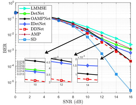
Figure 4: BER performance comparisons of DDNet with other MIMO detectors, testing at varying SNRs.

In this subsection, all networks are trained in the CL way. Fig. 4 compares the BER performance of the LMMSE, the SD [4], the AMP [5], the DetNet, the OAMPNet, the IDetNet and the DDNet detectors at varying SNRs. The IDetNet detector can achieve better BER performance than the DetNet detector, and the performance gain increases as SNR increases, which validates the effectiveness of the improvement skills in Section III-A. Furthermore, the IDetNet detector outperforms all other detectors except for the DDNet and the SD detectors when SNR is lower than 12 dB. The OAMPNet detector outperforms all other detectors except for the DDNet and the SD detectors when SNR is higher than 12 dB. Moreover, the DDNet detector consistently outperforms all other detectors except for the SD detector at all SNRs, and its performance gain compared to the upper bound of the IDetNet and the OAMPNet detectors is more significant when the performance of the IDetNet and the OAMPNet detectors is closer, as illustrated in the three enlarge pictures. This is because when the performance gap between the IDetNet and the OAMPNet detectors is wide at a certain SNR, the subnetwork RouteNet of the DDNet detector basically selects the definitely better one between IDetNet and OAMPNet for the testing samples at the certain SNR. Therefore the DDNet detector only achieves slight performance gains over the better one among the IDetNet and the OAMPNet detectors. In contrast, when the performance gap between the IDetNet and the OAMPNet detectors is narrow, the sample-wise dynamic routing among IDetNet and OAMPNet would bring more significant performance gains to the DDNet detector.

TABLE III: Average FLOPs of the detectors

Detector	LMMSE	IDetNet	OAMPNet	DDNet (12 dB)	DDNet (16 dB)	DDNet ($0\sim 16$ dB)
Flops ($1e5$)	1.61	6.00	55.66	8.1	16.3	9.2

Moreover, we calculate the average number of floating point operations (FLOPs), including multiplications and divisions, required for one sample with various detectors, as shown in Tab. III. The average number of FLOPs required for the DDNet detector increases as SNR increases because the OAMP subnetwork is more likely to be activated as SNR increases. As shown in Fig. 4 and Tab. III, the proposed DDNet detector could achieve better performance than the OAMP detector with much lower complexity.

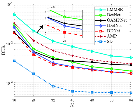
Figure 5: BER performance comparisons of DDNet with other MIMO detectors, testing at varying values of $N_{r}$.

Fig. 5 compares the BER performance of the LMMSE, the SD, the AMP, the DetNet, the OAMPNet, the IDetNet and the DDNet detectors at varying values of $N_{r}$ and SNR = 10 dB. The performance of all the detectors improves as $N_{r}$ increases and the IDetNet detector consistently outperforms the DetNet detector as $N_{r}$ increases. Moreover, the IDetNet detector outperforms all other detectors except for the DDNet and the SD detectors when $N_{r}$ is larger than 24 while the OAMPNet detector outperforms all other detectors except for the DDNet and the SD detectors when $N_{r}$ is smaller than about 24. Similar with Fig. 4, the DDNet detector outperforms all other detectors except for the SD detector. Thanks to the sample-wise dynamic routing of DDNet, the performance gain of the DDNet detector compared to the upper bound of the IDetNet and the OAMPNet detectors is more significant when the performance of the IDetNet and the OAMPNet detectors is closer.

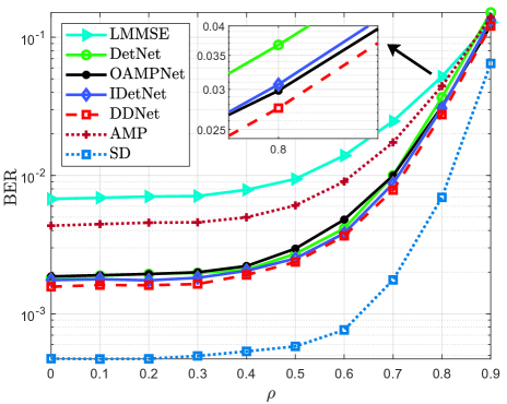
Figure 6: BER performance comparisons of DDNet with other MIMO detectors, testing at varying correlation coefficient $\rho$.

Fig. 6 compares the BER performance of the LMMSE, the SD, the AMP, the DetNet, the OAMPNet, the IDetNet and the DDNet detectors at varying values of correlation coefficient $\rho$ and SNR = 10 dB. The performance of all the detectors degrades as $\rho$ increases, and the IDetNet detector consistently outperforms the DetNet detector as $\rho$ increases. As shown in the enlarge picture, the IDetNet detector outperforms all other detectors except for the DDNet and the SD detectors when $\rho$ is smaller than 0.8 while the OAMPNet detector outperforms all other detectors except for the DDNet and the SD detectors when $\rho$ is larger than 0.8. As displayed in Fig. 4 $\sim$ Fig. 6, the DDNet detector consistently outperforms all other detectors except for the SD detector under all system conditions, which validates the effectiveness and the superiority of the sample-wise dynamic routing in the DDNet detector.

V-C The FedAve-DDNet Detector

Tab. IV investigates the impact of varying $M_{\mathrm{ID}}$ and $M_{\mathrm{RO}}$ on the federated training of IDetNet and RouteNet, where the number of local updates $\ell_{m}$ is set to be 2. We recode the epoch numbers of the IDetNet detector required to reach BER$<10^{-2}$ and the epoch numbers of RouteNet required to achieve convergence. It can be seen that a larger number of selected clients leads to faster convergence but lower computational efficiency. Therefore, we respectively set $M_{\mathrm{ID}}$ and $M_{\mathrm{RO}}$ to be 8 and 16 to strike a balance between the computational efficiency and the convergence rate.

TABLE IV: The impact of varying $M_{\mathrm{ID}}$ and $M_{\mathrm{RO}}$ on the training of IDetNet and RouteNet.

$M_{\mathrm{ID}}$		4	8	16	32	$M_{\mathrm{RO}}$		4	8	16	32
Epoches (BER$<10^{-2}$)	${D}_{m}^{\textrm{D}}=64$	430	240	180	150	Epoches (Convergence)	${D}_{m}^{\textrm{R}}=64$	125	80	40	25
	${D}_{m}^{\textrm{D}}=128$	380	200	140	110		${D}_{m}^{\textrm{R}}=128$	120	75	40	25

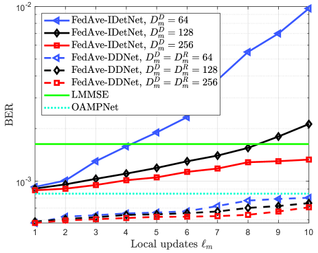
Figure 7: BER performance of the FedAve-DDNet and the FedAve-IDetNet detectors versus the number of local updates $\ell_{m}$.

Fig. 7 displays the BER performance of the FedAve-DDNet and FedAve-IDetNet detectors versus the number of local updates $\ell_{m}$, where the notation “FedAve-” is added to indicate that the detector is trained based on the FedAve algorithm. Note that when $\ell_{m}$ is 1, the FedAve algorithm is actually equivalent to the CL training with its batch size equal to the selected client number multiplied by the local dataset size. The performance of the FedAve-DDNet and the FedAve-IDetNet detectors degrades as $\ell_{m}$ increases while the declining slope decreases as the number of local samples ${D}_{m}^{\textrm{D}}$ increases. This is because that $\ell_{m}$ successive parameter-updates on the local datasets lead to overfitting, and a smaller ${D}_{m}^{\textrm{D}}$ results in more serious overfitting. Moreover, the LMMSE and the CL based OAMPNet detectors, represented by two horizontal lines, are used as the benchmarks. It can be seen that the FedAve-IDetNet detector could exhibit worse performance when $\ell_{m}$ is greater than a certain value. Furthermore, the FedAve-DDNet detector consistently outperforms the OAMPNet detector while their performance gap becomes narrower as $\ell_{m}$ increases. This is because that the performance gap between the FedAve-IDetNet and OAMPNet detectors becomes wider as $\ell_{m}$ increases, which indicates that it would be more difficult for the FedAve-DDNet detector to benefit from the sample-wise dynamic routing among the FedAve-IDetNet and OAMPNet. Notice that the varying $\ell_{m}$ has more moderate impacts on the FedAve-DDNet detector than the FedAve-IDetNet detector, which is due to the stabilization of the CL based OAMPNet detector. It should be mentioned that although the datasets ${\mathbb{D}}_{m}^{\textrm{D}}$ and ${\mathbb{D}}_{m}^{\textrm{R}}$ may not have the same number of samples in actual implementations according to the Section III-C, we set ${\mathbb{D}}_{m}^{\textrm{D}}={\mathbb{D}}_{m}^{\textrm{R}}$ in order to control variable effects, i.e., to better compare the robustness of the FedAve-DDNet and the FedAve-IDetNet detectors over $\ell_{m}$.

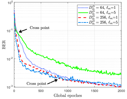
Figure 8: BER performance of the FedAve-IDetNet detector versus the number of global epoches.

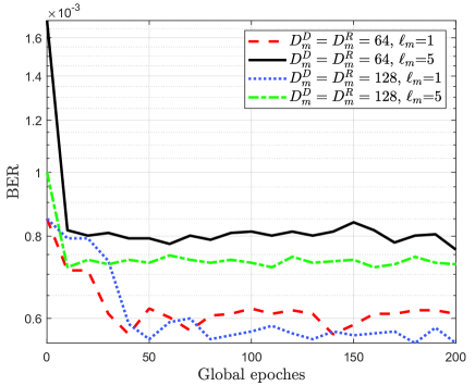
Figure 9: BER performance of the FedAve-DDNet detector versus the number of global epoches while training RouteNet.

Fig. 9 shows the BER performance of the FedAve-IDetNet detectors versus the number of global epoches with varying $\ell_{m}$ and ${\mathbb{D}}_{m}^{\textrm{D}}$. The BERs of the FedAve-IDetNet detectors decrease as the number of global epoches increases, and the declining slopes also decrease as the number of global epoches increases. Notice that the FedAve-IDetNet detectors with $\ell_{m}=5$ first decrease faster but then decrease slower than those with $\ell_{m}=1$. The cross point for the FedAve-IDetNet detectors with $D_{m}=64$ occurs during the 80-th global epoches while the cross point for the FedAve-IDetNet detectors with $D_{m}=256$ occurs during the 800-th global epoches. Since there is a positive correlation between the transmission overhead and the number of global epoches as indicated by Eq. (43), we can find that more local updates per global epoch could reduce the transmission overhead in the early stage of training. However, this advantage becomes insignificant when ${\mathbb{D}}_{m}^{\textrm{D}}$ is small, because that a small local dataset is more likely to be over-optimized by local updates, which leads to a premature cross point of the BER curves.

Fig. 9 displays the BER performance of the FedAve-DDNet detector versus the number of global epoches in the federated training process of RouteNet with varying $\ell_{m}$, ${D}_{m}^{\textrm{D}}$ and ${D}_{m}^{\textrm{R}}$. It can be seen that the FedAve-DDNet detectors with $\ell_{m}=1$ converge after training RouteNet 40 global epoches while the FedAve-DDNet detectors with $\ell_{m}=5$ converge only after 10 global epoches. Moreover, the value of ${\mathbb{D}}_{m}^{\textrm{D}}$ or ${D}_{m}^{\textrm{R}}$ almost has no impact on the convergence rate. This is because that RouteNet has certain tendency of dynamic routing for a certain client, which implies that the datasets of different clients, i.e., ${\mathbb{D}}_{m}^{\textrm{R}}$, are highly non-i.i.d.. In this case, the route labels of a certain client are seriously unbalanced, and thus it would be inefficient to increase the sample number of the local dataset ${\mathbb{D}}_{m}^{\textrm{R}}$ to improve the training performance.

As illustrated in Fig. 7 $\sim$ Fig. 9, the detectors with larger $\ell_{m}$ converge faster in the early stage of training but achieve worse convergence performance. Therefore, a experienced engineer could fine-tune the value of $\ell_{m}$ to improve the converge speed and the final accuracy, i.e., selecting larger $\ell_{m}$ at first and decreasing $\ell_{m}$ gradually.

V-D The FedGS-DDNet Detector

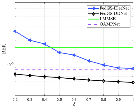
Figure 10: BER performance of the FedGS-DDNet and FedGS-IDetNet detectors versus the value of $\delta$. ${D}_{m}^{\textrm{D}}=256$. ${D}_{m}^{\textrm{R}}=128$.

Fig. 10 displays the BER performance of the FedGS-DDNet and FedGS-IDetNet detectors versus the value of $\delta$, where the notation “FedGS-” is added to indicate that the detector is trained based on the FedGS algorithm. When $\delta$ is smaller than 0.4, the FedGS-IDetNet detector achieves worse performance than the LMMSE detector. Moreover, the FedGS-DDNet detector consistently outperforms the OAMPNet detector while their performance gap becomes wider as $\delta$ increases, which also implies that the FedGS-DDNet benefits from the improvements of the FedGS-IDetNet detector. Moreover, the accuracy of both the FedGS-DDNet and the FedGS-IDetNet detectors decrease as $\delta$ decreases. By selecting a proper $\delta$, the proposed FedGS-IDetNet and FedGS-DDNet detectors can strike a good balance between the accuracy and the transmission overhead.

V-E Transmission Overhead

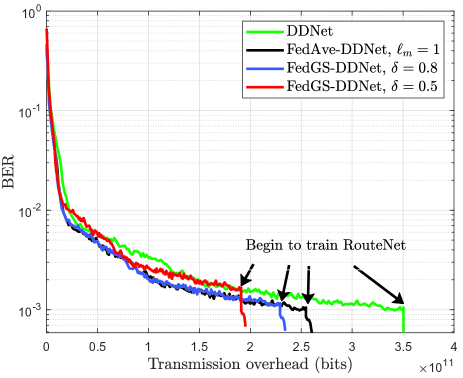
Figure 11: The BER curves of the CL-DDNet, the FedAve-DDNet, and the FedGS-DDNet detectors versus the transmission overhead. ${D}_{m}^{\textrm{D}}=256$. ${D}_{m}^{\textrm{R}}=128$. $b=32$ bits.

Fig. 11 draws the BER curves of the CL-DDNet, the FedAve-DDNet, and the FedGS-DDNet detectors versus the transmission overhead. Note that we normally begin the training process of CL algorithms after the whole dataset is collected and stuffed at the central server. However, here we assume that the dataset collection and the training are carried out in parallel during the CL training in order to intuitively compare the performance gains of the transmission overhead. In other words, Fig. 11 can be approximately interpreted as the BER performance of the above-mentioned detectors versus the number of global epoches since the transmission overheads of both the datasets and the network parameters are positively correlated with the number of global epoches during the training of IDetNet. Note that the curve of CL-DDNet becomes vertical when we begin to train the RouteNet since the whole route dataset can be generated in the central server based on the trained subnetworks and the whole dataset ${\mathbb{D}}_{\textrm{whole}}$, thus requiring no additional transmission overhead. As shown in Fig. 11, the FedAve-DDNet detector could reduce the transmission overhead by at least 25.7% while maintaining satisfactory detection accuracy. Moreover, the FedGS-DDNet detector could further reduce the transmission overhead at the cost of small accuracy loss.

VI Conclusion

In this paper, we designed the architecture of the DDNet detector based on the sample-wise dynamic routing among IDetNet and OAMPNet. By utilizing FL algorithms, we also proposed the FedAve-DDNet and the FedGS-DDNet detectors to reduce the transmission overhead and protect the data privacy. Simulation results have shown that the proposed DDNet detector could achieve better accuracy than both the IDetNet and the OAMPNet detectors under all system conditions, which validates the superiority of the sample-wise dynamic routing. Furthermore, the federated DDNet detectors, especially the FedGS-DDNet detector, can significantly reduce the transmission overhead while protecting the data privacy and maintain satisfactory accuracy.

References

- [1] B. Wang, F. Gao, S. Jin, H. Lin, G. Y. Li, S. Sun, and T. S. Rappaport, “Spatial-wideband effect in massive MIMO with application in mmwave systems,” IEEE Commun. Mag., vol. 56, no. 12, pp. 134–141, Dec. 2018.
- [2] B. Wang, F. Gao, S. Jin, H. Lin, and G. Y. Li, “Spatial- and frequency-wideband effects in millimeter-wave massive MIMO systems,” IEEE Trans. Signal Process., vol. 66, no. 13, pp. 3393–3406, Jul. 2018.
- [3] E. G. Larsson, “MIMO detection methods: How they work,” IEEE Signal Process. Mag., vol. 26, no. 3, pp. 91–95, Apr. 2009.
- [4] B.M. Hochwald and S. T. Brink, “Achieving near-capacity on a multiple-antenna channel,” IEEE Trans. Commun., vol. 51, no. 3, Mar. 2003.
- [5] S. Wu, L. Kuang, Z. Ni, J. Lu, D. Huang, and Q. Guo, “Low-complexity iterative detection for large-scale multiuser MIMO-OFDM systems using approximate message passing,” IEEE J. Selected Topics Signal Process., vol. 8, no. 5, pp. 902–915, Oct. 2014.
- [6] Z. Q. Luo, W. K. Ma, A. M. So, Y. Ye, and S. Zhang, “Semidefinite relaxation of quadratic optimization problems,” IEEE Signal Process. Mag., vol. 27, no. 3, pp. 20–34, Apr. 2010.
- [7] S. Yang and L. Hanzo, “Fifty years of MIMO detection: The road to large-scale MIMOs,” IEEE Commun. Surveys & Tutorials, vol. 17, no. 4, pp. 1941–1988, Sep. 2015.
- [8] H. He, C. Wen, S. Jin, and G. Y. Li, “Deep learning-based channel estimation for beamspace mmwave massive MIMO systems,” IEEE Wireless Commun. Lett., vol. 7, no. 5, pp. 852–855, Oct. 2018.
- [9] P. Dong, H. Zhang, G. Y. Li, I. S. Gaspar, and N. NaderiAlizadeh, “Deep CNN-based channel estimation for mmwave massive MIMO systems,” IEEE J. Sel. Topics Signal Process., vol. 13, no. 5, pp. 989–1000, Sep. 2019.
- [10] C. Wen, W. Shih, and S. Jin, “Deep learning for massive MIMO CSI feedback,” IEEE Wireless Commun. Lett., vol. 7, no. 5, pp. 748–751, Oct. 2018.
- [11] Y. Yang, F. Gao, G. Y. Li, and M. Jian, “Deep learning based downlink channel prediction for FDD massive MIMO system,” IEEE Commun. Lett., vol. 23, no. 11, pp. 1994–1998, Nov. 2019.
- [12] Y. Yang, F. Gao, X. Ma, and S. Zhang, “Deep learning-based channel estimation for doubly selective fading channels,” IEEE Access, vol. 7, pp. 36579–36589, Mar. 2019.
- [13] M. Alrabeiah and A. Alkhateeb, “Deep learning for TDD and FDD massive MIMO: Mapping channels in space and frequency,” in Proc. 53rd Asilomar Conf. Signals, Systems, Computers, California, USA, 2019, pp. 1465–1470.
- [14] Y. Yang, F. Gao, C. Qian, and G. Liao, “Model-aided deep neural network for source number detection,” IEEE Signal Process. Lett., vol. 27, pp. 91–95, Jan. 2020.
- [15] Q. Hu, F. Gao, H. Zhang, S. Jin, and G. Y. Li, “Deep learning for channel estimation: Interpretation, performance, and comparison,” IEEE Trans. Wireless Commun., vol. 20, no. 4, pp. 2398–2412, Dec. 2021.
- [16] Q. Hu, F. Gao, H. Zhang, G. Y. Li, and Z. Xu, “Understanding deep MIMO detection,” arXiv preprint arXiv:2105.05044, 2021.
- [17] N. Samuel, T. Diskin, and A. Wiesel, “Learning to detect,” IEEE Trans. Signal Process., vol. 67, no. 10, pp. 2554–2564, Feb. 2019.
- [18] H. He, C. Wen, S. Jin, and G. Y. Li, “Model-driven deep learning for MIMO detection,” IEEE Trans. Signal Process., vol. 68, pp. 1702–1715, Feb. 2020.
- [19] H. Ye, G. Y. Li, and B. Juang, “Power of deep learning for channel estimation and signal detection in OFDM systems,” IEEE Wireless Commun. Lett., vol. 7, no. 1, pp. 114–117, Feb. 2018.
- [20] J. Sun, Y. Zhang, J. Xue, and Z. Xu, “Learning to search for MIMO detection,” IEEE Trans. Wireless Commun., vol. 19, no. 11, pp. 7571–7584, Aug. 2020.
- [21] J. Liao, J. Zhao, F. Gao, and G. Y. Li, “A model-driven deep learning method for massive MIMO detection,” IEEE Commun. Lett., vol. 24, no. 8, pp. 1724–1728, Apr. 2020.
- [22] X. Tan, W. Xu, K. Sun, Y. Xu, Y. Beéry, X. You, and C. Zhang, “Improving massive MIMO message passing detectors with deep neural network,” IEEE Trans. Vehicular Technol., vol. 69, no. 2, pp. 1267–1280, Dec. 2020.
- [23] G. Gao, C. Dong, and K. Niu, “Sparsely connected neural network for massive MIMO detection,” in Proc. IEEE 4th Int. Conf. Computer Commun. (ICCC), Chengdu, China, 2018, pp. 397–402.
- [24] Y. Han, G. Huang, S. Song, L. Yang, H. Wang, and Y. Wang, “Dynamic neural networks: A survey,” arXiv preprint arXiv:2102.04906, 2021.
- [25] S. Sabour, N. Frosst, and G. E. Hinton, “Dynamic routing between capsules,” in Proc. 31st Int. Conf. Neural Information Process. Systems (NIPS), California, USA, 2017, pp. 3859–3869.
- [26] W. Fedus, B. Zoph, and N. Shazeer, “Switch transformers: Scaling to trillion parameter models with simple and efficient sparsity,” arXiv preprint arXiv:2101.03961.
- [27] Y. Yang, F. Gao, C. Xing, J. An, and A. Alkhateeb, “Deep multimodal learning: Merging sensory data for massive MIMO channel prediction,” IEEE J. Selected Areas Commun., pp. 1–1, Dec. 2020.
- [28] J. Guo, C. Wen, S. Jin, and G. Y. Li, “Convolutional neural network based multiple-rate compressive sensing for massive MIMO CSI feedback: Design, simulation, and analysis,” IEEE Trans. Wireless Commun., vol. 19, no. 4, pp. 2827–2840, Apr. 2020.
- [29] Y. Yang, F. Gao, Z. Zhong, B. Ai, and A. Alkhateeb, “Deep transfer learning based downlink channel prediction for FDD massive MIMO systems,” IEEE Trans. Commun., vol. 68, no. 12, pp. 7485–7497, Dec. 2020.
- [30] J. Guo, J. Wang, C. Wen, S. Jin, and G. Y. Li, “Compression and acceleration of neural networks for communications,” IEEE Wireless Commun., vol. 27, no. 4, pp. 110–117, Aug. 2020.
- [31] W. Xu, F. Gao, S. Jin, and A. Alkhateeb, “3D scene based beam selection for mmwave communications,” IEEE Wireless Commun. Lett., vol. 9, no. 11, pp. 1850–1854, Jun. 2020.
- [32] H. Ye, F. Gao, J. Qian, H. Wang, and G. Y. Li, “Deep learning-based denoise network for CSI feedback in FDD massive MIMO systems,” IEEE Commun. Lett., vol. 24, no. 8, pp. 1742–1746, Aug. 2020.
- [33] Z. Qin, H. Ye, G. Y. Li, and B. F. Juang, “Deep learning in physical layer communications,” IEEE Wireless Commun., vol. 26, no. 2, pp. 93–99, Apr. 2019.
- [34] H. Ye, L. Liang, G. Y. Li, and B. H. Juang, “Deep learning-based end-to-end wireless communication systems with conditional GANs as unknown channels,” IEEE Trans. Wireless Commun., vol. 19, no. 5, pp. 3133–3143, Feb. 2020.
- [35] S. Niknam, H. S. Dhillon, and J. H. Reed, “Federated learning for wireless communications: Motivation, opportunities, and challenges,” IEEE Commun. Mag., vol. 58, no. 6, pp. 46–51, Jul. 2020.
- [36] H. B. McMahan, E. Moore, D. Ramage, S. Hampson, and B. A. Arcas, “Communication-efficient learning of deep networks from decentralized data,” arXiv preprint arXiv:1602.05629, 2017.
- [37] T. Li, A. K. Sahu, M. Zaheer, M. Sanjabi, A. Talwalkar, and V. Smith, “Federated optimization in heterogeneous networks,” arXiv preprint arXiv:1812.06127, 2018.
- [38] Y. Kim, E. A. Hakim, J. Haraldson, H. Eriksson, J. M. B. Silva, and C. Fischione, “Dynamic clustering in federated learning,” in Proc. IEEE Int. Conf. Commun. (ICC), Montreal, QC, Canada, 2021, pp. 1–6.
- [39] Z. Qin, G. Y. Li, and H. Ye, “Federated learning and wireless communications,” arXiv preprint arXiv:2005.05265, 2020.
- [40] A. M. Elbir and S. Coleri, “Federated learning for channel estimation in conventional and irs-assisted massive MIMO,” arXiv preprint arXiv:2008.10846, 2020.
- [41] A. M. Elbir and S. Coleri, “Federated learning for hybrid beamforming in mm-wave massive MIMO,” IEEE Commun. Lett., vol. 24, no. 12, pp. 2795–2799, Dec. 2020.
- [42] D. Ma, L. Li, H. Ren, D. Wang, X. Li, and Z. Han, “Distributed rate optimization for intelligent reflecting surface with federated learning,” in Proc. IEEE Int. Conf. Commun. Workshops (ICC Workshops), Dublin, Ireland, 2020, pp. 1–6.
- [43] Y. Zhou, Y. Qing, and J. Lv, “Communication-efficient federated learning with compensated overlap-fedavg,” arXiv preprint arXiv:2012.06706, 2020.
- [44] X. Li, K. Huang, W. Yang, S. Wang, and Z. Zhang, “On the convergence of fedavg on non-iid data,” in Proc. Int. Conf. Learning Representations (ICLR), Louisiana, United States, 2019, pp. 1–6.
- [45] Y. Lin, S. Han, H. Mao, Y. Wang, and B. Dally, “Deep gradient compression: Reducing the communication bandwidth for distributed training,” in Proc. Int. Conf. Learning Representations (ICLR), Vancouver, Canada, 2018, pp. 1–6.
- [46] J. Wangni, J. Wang, J. Liu, and T. Zhang, “Gradient sparsification for communication-efficient distributed optimization,” in Proc. 32nd Int. Conf. Neural Information Process. Systems, Montréal, Canada, 2018, pp. 1306–1316.
- [47] D. Kingma and J. Ba, “Adam: A method for stochastic optimization,” arXiv preprint arXiv:1412.6980, 2014.
- [48] Yurii Nesterov, “Introductory lectures on convex programming volume i: Basic course,” Lecture notes, vol. 3, no. 4, pp. 5, 1998.
- [49] H. Ye, G. Y. Li, and B. H. Juang, “Deep learning based end-to-end wireless communication systems without pilots,” IEEE Trans. Cognitive Commun. Networking, pp. 1–1, Feb. 2021.