An Efficient Semismooth Newton Method for Adaptive Sparse Signal Recovery Problems

Abstract

We know that compressive sensing can establish stable sparse recovery results from highly undersampled data under a restricted isometry property condition. In reality, however, numerous problems are coherent, and vast majority conventional methods might work not so well. Recently, it was shown that using the difference between $\ell_{1}$- and $\ell_{2}$-norm as a regularization always has superior performance. In this paper, we propose an adaptive $\ell_{p}$-$\ell_{1-2}$ model where the $\ell_{p}$-norm with $p\geq 1$ measures the data fidelity and the $\ell_{1-2}$-term measures the sparsity. This proposed model has the ability to deal with different types of noises and extract the sparse property even under high coherent condition. We use a proximal majorization-minimization technique to handle the nonconvex regularization term and then employ a semismooth Newton method to solve the corresponding convex relaxation subproblem. We prove that the sequence generated by the semismooth Newton method admits fast local convergence rate to the subproblem under some technical assumptions. Finally, we do some numerical experiments to demonstrate the superiority of the proposed model and the progressiveness of the proposed algorithm.

Key words. Compressive sensing, $\ell_{p}$-$\ell_{1-2}$ minimization, proximal majorization-minimization, Clarke subdifferential, semismooth Newton method.

1 Introduction

It is well known that compressive sensing (CS) is a novel signal acquisition paradigm to sense sparse signals by acquiring a set of incomplete or even noises polluted measurements, and subsequently recovers the signals by solving an optimization problem. Let $\underline{x}\in\mathbb{R}^{n}$ be a compressible or (approximately) sparse signal under a suitable basis (e.g. Fourier or wavelet basis). The main idea of CS is to firstly project $\underline{x}$ onto a certain subspace via a linear operator $A$, i.e, $A\underline{x}=b$ with $b\in\mathbb{R}^{m}$ and $m\ll n$, and then reconstruct $\underline{x}$ from the undersampled data $b$ via finding the sparest solution of the following underdetermined linear system:

$$Ax=b.$$

Besides, in the process of acquiring, storing, transmitting, or displaying, the undersampled data may be inevitably degenerated by noise. In this case, it is from the basic theory of CS Candes and Tao (2005); Donoho (2006); Donoho and Elad (2003) that, the task of recovering $\underline{x}$ can be characterized as the following $\ell_{1}$-norm regularized least square

$$\min_{x\in\mathbb{R}^{n}}\frac{1}{2}\|Ax-b\|^{2}_{2}+\lambda\|x\|_{1},$$

where $\|\cdot\|_{1}$ is an $\ell_{1}$-norm function, and $\lambda>0$ is a weighting parameter to balance both terms for minimization. A deterministic result shows that it is possible to recover the original signal by $\ell_{1}$-norm minimization when the number of nonzeros of $\underline{x}$ is less than $(1+1/\zeta)/2$ Donoho and Elad (2003); Gribonval and Nielsen (2003), where $\zeta$ is the so-called mutual coherence of matrix $A$. This fact indicates that using the $\ell_{1}$-norm alone may not perform well for highly coherent matrices, and hence, some improvements are highly required.

A valid approach among such efforts is the using of the difference between the $\ell_{1}$- and $\ell_{2}$-norm as a regularization Lou et al. (2015); Lou and Yan (2018); Lou et al. (2015); Yin et al. (2015), which always has superior performance over the $\ell_{1}$-norm and even the $\ell_{q}$-norm with $q\in(0,1)$ alone Chen et al. (2014); Chen et al. (2010); Daubechies et al. (2009) in improving the sparsity when the sensing matrix $A$ is highly coherent. Based on the fact, the recovering task of $\underline{x}$ using $\ell_{1}$-$\ell_{2}$-norm can be explicitly formulated as

$$\min_{x\in\mathbb{R}^{n}}\frac{1}{2}\|Ax-b\|^{2}_{2}+\lambda(\|x\|_{1}-\|x\|_{2}),$$ (1.1)

where “$\|x\|_{1}-\|x\|_{2}$” (short for $\ell_{1-2}$) is called a regularization. It should be noted that despite having some attractive features as shown by Yin et al. Yin et al. (2015), the quality of the resolutions derived by model (1.1) heavily relies on the knowing of the standard deviation of the noise. Fortunately, the square-root-loss estimator of Belloni et al. Belloni et al. (2011), say $\|Ax-b\|_{2}$, is proved to be achieving the near-oracle rates of convergence without knowing the standard deviation of the noise under suitable design conditionsBellec et al. (2018); Cui et al. (2018). The data fidelity with form $\|Ax-b\|_{1}$ has also been evidently shown to be more robust when the noises are not normal but heavy-tailed or heterogeneous, see e.g., Belloni and Chernozhukov (2011); Lu (2014); Wang (2013); Xiu et al. (2018). Besides, the data fidelity with form $\|Ax-b\|_{\infty}$ is also known to be very suitable for dealing with the uniformly distributed noise and quantization error, see e.g., Wen et al. (2018); Xue et al. (2019); Zhang and Wei (2015). Therefore, a more natural question is whether or not one can design a more flexible and robust reconstruction model as well as an efficient algorithm which is capable of dealing with all the three types of noise mentioned above?

The main purpose of this paper is to answer the question positively in the sense of considering the following $\ell_{p}$-$\ell_{1-2}$ minimization problem

$$\min_{x\in\mathbb{R}^{n}}\|Ax-b\|_{p}+\lambda(\|x\|_{1}-\beta\|x\|_{2}),$$ (1.2)

where $\beta\geq 0$ and $\|\cdot\|_{p}$ is a $\ell_{p}$-norm function whose proximal mapping is assumed to be strongly semismooth, e.g., $p=1,2,\infty$ as stated in (Lin et al., 2020, Remark 2). The model (1.2) has many attractive features that, the $\|Ax-b\|_{p}$ data fidelity term makes it can deal with different types of noise if $p$ is chosen adaptively, and the $\ell_{1-2}$ regularization ensures the sparse property can be well extracted even under high coherent condition. For example, the choices of $p=1$, $2$ and $\infty$ is appropriate for log-normal noise or Laplace noise, Gaussian noise, and uniformly distributed noise, respectively. Nevertheless, comparing with (1.1), it is much more difficult and challenging to solve due to the non-differentiability of the $\ell_{p}$-norm along with the nonconvexity of the difference between the $\ell_{1}$-norm and $\ell_{2}$-norm.

Noting that the “$\|x\|_{1}-\beta\|x\|_{2}$” term is actually a difference of two convex functions, Yin et al. Yin et al. (2015) linearized the concave term “$-\|x\|_{2}$” at a given point to get a convex relaxation minimization problem, and then employed an alternating direction methods of multipliers on the resulting convex relaxation problem. Beside, Tang et al. Tang et al. (2020) added a pair of proximal terms to the convex problems, and then proposed an efficient semismooth Newton method. Inspired from both works of Tang et al. (2020); Yin et al. (2015), in this paper, we introduce an efficient proximal majorization-minimization semismooth Newton method algorithm to solve the general problem (1.2). Our algorithm firstly linearizes the concave term in (1.2) at current iteration to get a convex nonsmooth minimization, adds a pair of proximal terms to the objective function, and then uses an efficient semismooth Newton method to solve the involved semismooth nonlinear system to ensure faster local convergence rate. It should be noted that, the first contribution of this paper is that our model (1.2) covers the root-square-loss as a special case, which is more flexible than the model considered by Tang et al. Tang et al. (2020). Besides, we focus on a nonsmooth concave term“$-\|x\|_{2}$” but not a differentiable concave function as in Tang et al. (2020). We must clarify that, the diversification of the $\ell_{p}$-norm in (1.2) may make the positive definiteness of generalized Hessian at the solution be violated, which poses fundamental challenges to the design of efficient algorithms. The second contribution of this paper is to address this issue in the sense that, we employ the semismooth Newton method to solve the resulting subproblem with choices $p=1,2,\infty$, and prove that each limit point of the generated sequence converges to an optimal solution of the subproblem and admits fast local convergence rate under some technical assumptions. Finally, we do a series of numerical experiments which demonstrate that the superiority of the proposed model (1.2) is remarkable and the proposed algorithm is very efficient.

The remaining parts of this paper are organized as follows. In Section 2, we summarize some basic definitions or concepts for subsequent arithmetic design and numerical implementations. In Section 3, we give our motivation and construct our algorithm. Besides, the convergence result for the proposed algorithm is also included. Numerical experiments and performance comparisons are reported in Section 4. Finally, the paper is concluded with some remarks in Section 5 .

2 Preliminaries

Let $\mathbb{R}^{n}$ be an $n$-dimensional Euclidean space endowed with an inner product $\langle\cdot,\cdot\rangle$ and its induced norm $\|\cdot\|_{2}$, respectively. Let $f:\mathbb{R}^{n}\rightarrow(-\infty,+\infty]$ be a closed proper convex function. The effective domain of $f$, which we denote by $\text{dom}(f)$, is defined as $\text{dom}(f)=\{x|f(x)<+\infty\}$. The directional derivative of $f$ at a point $x\in\text{dom}(f)$ along a direction $d\in\mathbb{R}^{n}$ is defined as

$$f^{\prime}(x;d):=\lim_{\tau\downarrow 0}\frac{f(x+\tau d)-f(x)}{\tau}.$$

We say $\bar{x}\in\text{dom}(f)$ is the d-stationary point of $f$, if it satisfies $f^{\prime}(\bar{x};d)\geq 0$, $\forall d\in\mathbb{R}^{n}$. The Fenchel conjugate of $f$ at $x^{*}$ is defined by $f^{*}(x^{*}):=\sup_{x\in\mathbb{R}^{n}}\{\langle x,x^{*}\rangle-f(x)\}$.

Denote $\Phi_{tf}(x)$ be the Moreau envelope function Moreau (1964); Yosida (1964) of $f$ with parameter $t>0$, i.e.,

$$\Phi_{tf}(x):=\min_{y\in\mathbb{R}^{n}}\big{\{}f(y)+\frac{1}{2t}\|y-x\|_{2}^{2}\big{\}},\quad\forall x\in\mathbb{R}^{n}.$$

The proximal mapping of $f$ with $t>0$ is defined as

$$\operatorname{Prox}_{tf}(x):=\underset{y\in\mathbb{R}^{n}}{\operatorname{argmin}}\big{\{}f(y)+\frac{1}{2t}\|y-x\|_{2}^{2}\big{\}},\quad\forall x\in\mathbb{R}^{n}.$$

From Hiriart-Urruty and Lemarechal (2013); Lemarechal and Sagastizabal (1997), it is known that $\Phi_{tf}(x)$ is continuously differentiable and convex with its gradient being given by

$$\nabla\Phi_{tf}(x)=t^{-1}(x-\operatorname{Prox}_{tf}(x)),\quad\forall x\in\mathbb{R}^{n}.$$

Besides, from (Rockafellar, 1970, Theorem 35.1), we have the following famous Moreau’s identity theorem, which plays a key rule in the subsequent analysis

$$\text{Prox}_{tf}(x)+t\text{Prox}_{f^{*}/t}(x/t)=x.$$ (2.3)

Next we quickly review some basic concepts and definitions which are used frequently in the subsequent arithmetic developments and numerical implementations. Semismoothness was originally introduced by Miffin Mifflin (1977) for functionals, and the concept was extended to vector valued functions by Qi and Sun Qi and Sun (1993).

Definition 2.1.

(semismoothness Mifflin (1977); Qi and Sun (1993)). Let $\Psi:\mathcal{O}\subseteq\mathbb{R}^{n}\rightarrow\mathbb{R}^{m}$ be a locally Lipschitz contimuous function and $\mathcal{K}:\mathcal{O}\rightrightarrows\mathbb{R}^{m\times n}$ be a nonempty and compact valued, upper-semicontinuous set-valued mapping on the open set $\mathcal{O}$. It is said $\Psi$ to be semismooth at $\nu\in\mathcal{O}$ with respect to the set-valued mapping $\mathcal{K}$ if $\Psi$ is directionally differentiable at $\nu$ and for any $\Gamma\in\mathcal{K}(\nu+\Delta\nu)$ with $\Delta\nu\rightarrow 0$ such that

$$\Psi(\nu+\Delta\nu)-\Psi(\nu)-\Gamma\Delta\nu=o(\|\Delta\nu\|_{2}).$$

Besides, it is said $\Psi$ to be $\gamma$-order $(\gamma>0)$ (strongly, if $\gamma=1$ ) semismooth at $\nu$ with respect to $\mathcal{K}$ if $\Psi$ is semismooth at $\nu$ and for any $\Gamma\in\mathcal{K}(\nu+\Delta\nu)$ such that

$$\Psi(\nu+\Delta\nu)-\Psi(\nu)-\Gamma\Delta\nu=O(\|\Delta\nu\|_{2}^{1+\gamma}).$$

Moreover, we say that $\Psi$ is a semismooth $(\gamma$-order semismooth, strongly semismooth) function on $\mathcal{O}$ with respect to $\mathcal{K}$ if it is semismooth $(\gamma$-order semismooth, strongly semismooth) at every $\nu\in\mathcal{O}$ with respect to $\mathcal{K}$.

Theorem 2.1.

(Rademacher’s Theorem Rockafellar and Wets (1998)) Suppose that $\Psi:\mathbb{R}^{n}\rightarrow\mathbb{R}^{m}$ is locally Lipschitz continuous on an open set $\mathcal{O}\subseteq\mathbb{R}^{n}$. Then $\Psi$ is almost everywhere (in the sense of Lebesgue measure) Fréchet-differentiable in $\mathcal{O}$.

Let $\mathcal{D}_{\Psi}$ be the set of all points where $\Psi$ is Fréchet-differentiable and $J\Psi(x)\in\mathbb{R}^{m\times n}$ be the Jacobian of $\Psi$ at $x\in\mathcal{D}_{\Psi}$. For any $x\in\mathcal{O}$, the B-subdifferential of $\Psi$ at $x$ is defined by

$$\partial_{B}\Psi(x):=\{V\in\mathbb{R}^{m\times n}\mid\exists\{x^{k}\}\subseteq\mathcal{D}_{\Psi}\text{ such that }\lim_{k\rightarrow\infty}x^{k}=x\text{ and }\lim_{k\rightarrow\infty}J\Psi(x^{k})=V\}.$$

The Clarke Jacobian of $\Psi$ at $x$ is defined as the convex hull of the B-subdifferential of $\Psi$ at $x$, that is $\partial\Psi(x):=\text{conv}(\partial_{B}\Psi(x))$. For more detail, one may refer to Clarke (1983). Let $f$ be specially defined as $f:\mathbb{R}^{n}\rightarrow\mathbb{R}$. The Clarke subdifferential of $f$ at $x$ is defined as

$$\partial f(x):=\big{\{}h\in\mathbb{R}^{n}\mid\limsup_{x^{\prime}\rightarrow x,t\downarrow 0}\frac{f(x^{\prime}+ty)-f(x^{\prime})-th^{\top}y}{t}\geq 0,\forall y\in\mathbb{R}^{n}\big{\}}.$$

The regular subdifferential of $f$ at $x$ is defined as

$$\hat{\partial}f(x):=\big{\{}h\in\mathbb{R}^{n}\mid\liminf_{x\neq y\rightarrow x}\frac{f(y)-f(x)-h^{\top}(y-x)}{\|y-x\|_{2}}\geq 0\big{\}}.$$ (2.4)

Let $\Psi:\mathbb{R}^{n}\rightarrow\mathbb{R}^{n}$ is a locally Lipschitz continuous function. The generalized Newton’s method for solving $\Psi(x)=0$ was firstly proposed by Kummer Kummer (1988). Correspondingly, one can refer to (Qi, 1993, Theorem 3.1) and (Qi and Sun, 1993, Theorem 3.4) for its local convergence analysis at the case of $\Psi$ being semismooth. The most distinctive feature of the inexact semismooth Newton method is to find an approximate solution $d^{k}$ to

$$\Psi(x^{k})+V^{k}d=0,$$

such that

$$\|\Psi(x^{k})+V^{k}d^{k}\|\geq\eta\|\Psi(x^{k})\|,$$

where $V^{k}\in\partial\Psi(x^{k})$ and $\eta>0$ is a small constant. It was shown that when the elements in $\partial\Psi(\bar{x})$ are nonsingluar and $\Psi$ is semismooth at solution $\bar{x}$, the generated sequence $\{x^{k}\}$ is well-defined and converges to $\bar{x}$ suplinearly and even quadratic for $k$ sufficiently large. For more details of inexact semismooth Newton method, one can refer to Facchinei and Kanzow (1997); Martinez and Qi (1995) and the references therein.

Let $B^{(r)}_{p}$ be a $\ell_{p}$-norm ball with radius $r>0$ and define $\Pi_{B^{(r)}_{p}}(\cdot)$ be an orthogonal projection onto $B^{(r)}_{p}$. Using this notation, we summarize some proximal mappings of norm functions, which play key rules in the algorithmic construction. The following Lemma 2.1 reports some applications of the Moreau’s identity (2.3) for some typical norm functions. These results are known in optimization literature, hence, we omit its proof here.

Lemma 2.1.

For any $x^{*}\in\mathbb{R}^{n}$, it holds that
(a) Let $f(x):=\mu\|x\|_{1}$ with $\mu>0$, then $f^{*}(x^{*})=\delta_{B^{(\mu)}_{\infty}}(x^{*})$ with ${B^{(\mu)}_{\infty}}(x^{*}):=\{x^{*}\ |\ \|x^{*}\|_{\infty}\leq\mu\}$ and

$$\operatorname{Prox}_{f}(x^{*})=x^{*}-\Pi_{B^{(\mu)}_{\infty}}(x^{*})\quad\text{with}\quad(\Pi_{B^{(\mu)}_{\infty}}(x^{*}))_{i}=\left\{\begin{array}[]{ll}x^{*}_{i},&\text{ if }|x^{*}_{i}|\leq\mu,\\ \operatorname{sign}(x^{*}_{i})\mu,&\text{ if }|x^{*}_{i}|>\mu,\end{array}\right.$$

where $i=1,\ldots,n$ and $sign(\cdot)$ is a sign function of a vector.
(b) Let $f(x):=\mu\|x\|_{2}$ with $\mu>0$, then $f^{*}(x^{*})=\delta_{B^{(\mu)}_{2}}(x^{*})$ with ${B^{(\mu)}_{2}}(x^{*}):=\{x^{*}\ |\ \|x^{*}\|_{2}\leq\mu\}$ and

$$\operatorname{Prox}_{f}(x^{*})=x^{*}-\Pi_{B^{(\mu)}_{2}}(x^{*})\quad\text{with}\quad\Pi_{B^{(\mu)}_{2}}(x^{*})=\left\{\begin{array}[]{ll}x^{*},&\text{ if }\|x^{*}\|_{2}\leq\mu,\\ \mu\frac{x^{*}}{\|x^{*}\|_{2}},&\text{ if }\|x^{*}\|_{2}>\mu.\end{array}\right.$$

(c) Lin et al. (2020) Let $f(x):=\mu\|x\|_{\infty}$ with $\mu>0$, then $f^{*}(x^{*})=\delta_{B^{(\mu)}_{1}}(x^{*})$ with ${B^{(\mu)}_{1}}(x^{*}):=\{x^{*}\ |\ \|x^{*}\|_{1}\leq\mu\}$ and

$$\operatorname{Prox}_{f}(x^{*})=x^{*}-\Pi_{B^{(\mu)}_{1}}(x^{*})\quad\text{with}\quad\Pi_{B^{(\mu)}_{1}}(x^{*})=\left\{\begin{array}[]{ll}x^{*},&\text{ if }\|x^{*}\|_{1}\leq\mu,\\ \mu P_{x^{*}}\Pi_{\Delta_{n}}\left(P_{x^{*}}x^{*}/\mu\right),&\text{ if }\|x^{*}\|_{1}>\mu.\end{array}\right.$$

where $P_{x^{*}}:=\operatorname*{Diag}(\operatorname{sign}(x^{*}))$ and $\Pi_{\Delta_{n}}(\cdot)$ denotes the projection onto the simplex $\Delta_{n}:=\{x\in\mathbb{R}^{n}\mid e_{n}^{\top}x=1,x\geq 0\}$, in which $\operatorname*{Diag}(\cdot)$ denotes a diagonal matrix with elements of a given vector on its diagonal positions.

The following Lemma 2.2 characterizes the Clarke Jacobian of proximal mapping operators regarding to some special norm functions. The third part of this lemma is recently obtained by Li et al. Lin et al. (2020).

Lemma 2.2.

For any $\vartheta\in\mathbb{R}^{n}$, it holds that
(a) The Clarke Jacobian of $\operatorname{Prox}_{f}(\cdot)$ with $f(x):=\mu\|x\|_{1}$ at $\vartheta$ is given by

$$\partial\operatorname{Prox}_{f}(\vartheta)=\bigg{\{}\operatorname*{Diag}(\theta)\Big{|}\theta\in\mathbb{R}^{n},\ \theta_{i}\in\left\{\begin{array}[]{ll}\{1\},&\text{ if }|\vartheta_{i}|>\mu,\\ {[}0,1{]},&\text{ if }|\vartheta_{i}|=\mu,\quad i=1,\ldots,n\\ \{0\},&\text{ if }|\vartheta_{i}|<\mu,\end{array}\right.\bigg{\}}.$$

(b) The Clarke Jacobian of $\operatorname{Prox}_{f}(\cdot)$ with $f(x):=\mu\|x\|_{2}$ at $\vartheta$ is given by

$$\partial\operatorname{Prox}_{f}(\vartheta)=\left\{\begin{array}[]{ll}(1-\dfrac{\mu}{\|\vartheta\|_{2}})\mathbf{I}_{n}+\mu\dfrac{\vartheta\vartheta^{\top}}{\|\vartheta\|_{2}^{3}},&\text{ if }\|\vartheta\|_{2}>\mu,\\[5.69054pt] \{\kappa\dfrac{\vartheta\vartheta^{\top}}{\mu^{2}}\mid 0\leq\kappa\leq 1\},&\text{ if }\|\vartheta\|_{2}=\mu,\\[5.69054pt] \mathbf{0}_{n},&\text{ if }\|\vartheta\|_{2}<\mu,\end{array}\right.$$

where $\mathbf{I}_{n}$ and $\mathbf{0}_{n}$ are identify matrix and zero matrix in $n$-dimensional Euclidean space, respectively.
(c)Lin et al. (2020) The Clarke Jacobian of $\operatorname{Prox}_{f}(\cdot)$ with $f(x):=\mu\|x\|_{\infty}$ at $\vartheta$ is given by

$$\partial\operatorname{Prox}_{f}(\vartheta)=\mathbf{I}_{n}-H,$$

where $H\in\partial\Pi_{B^{(\mu)}_{1}}(\vartheta)$ with explicit form

$$H=\left\{\begin{array}[]{ll}P_{\vartheta}\tilde{H}P_{\vartheta},&\text{ if }\|\vartheta\|_{1}>\mu,\\ \mathbf{I}_{n},&\text{ if }\|\vartheta\|_{1}\leq\mu,\end{array}\right.$$

where $\tilde{H}=\text{Diag}(r)-\frac{1}{nnz(r)}rr^{\top}\in\partial\Pi_{\Delta_{n}}(\vartheta)$ with $r\in\mathbb{R}^{n}$ defined as $r_{i}=1$ if $\left(\Pi_{\Delta_{n}}\left(P_{\vartheta}\vartheta/\mu\right)\right)_{i}\neq 0,$ and $r_{i}=0$ otherwise, and $\text{nnz}(\cdot)$ denotes the number of non-zeros elements of a vector.

It is noteworthy that, we specifically formalize the element of $\operatorname{Prox}_{f}(\cdot)$ at each case for the purpose of catching the subsequent algorithm’s development easily.

Remark 2.1.

In our numerical experiments part, we choose the element $\hat{\Theta}$ in $\partial\operatorname{Prox}_{\mu\|\cdot\|_{1}}(\vartheta)$ at a given point $\vartheta$ as

$$\hat{\Theta}=\operatorname{diag}(\theta)\text{ with }\theta_{i}=\left\{\begin{array}[]{ll}1,&\text{ if }\left|\vartheta_{i}\right|>\mu,\\[5.69054pt] 0,&\text{ if }\left|\vartheta_{i}\right|\leq\mu,\quad i=1,\ldots,n,\end{array}\right.$$

choose the element $\hat{\Theta}$ in $\partial\operatorname{Prox}_{\mu\|\cdot\|_{2}}(\vartheta)$ as

$$\hat{\Theta}=\left\{\begin{array}[]{ll}(1-\dfrac{\mu}{\|\vartheta\|_{2}})\mathbf{I}_{n}+\mu\dfrac{\vartheta\vartheta^{\top}}{\|\vartheta\|_{2}^{3}},&\text{ if }\|\vartheta\|_{2}>\mu,\\ \mathbf{0}_{n},&\text{ if }\|\vartheta\|_{2}\leq\mu,\end{array}\right.$$

and choose the element $\hat{\Theta}$ in $\partial\operatorname{Prox}_{\mu\|\cdot\|_{\infty}}(\vartheta)$ as

$$\hat{\Theta}=\left\{\begin{array}[]{ll}\mathbf{I}_{n}-P_{\vartheta}\tilde{H}P_{\vartheta},&\text{ if }\|\vartheta\|_{1}>\mu,\\[5.69054pt] \mathbf{0}_{n},&\text{ if }\|\vartheta\|_{1}\leq\mu,\end{array}\right.$$

where $\tilde{H}$ is defined in (c) of Lemma 2.2.

3 Computational approach

This section is devoted to constructing a new algorithm to solve the model (1.2). Similar to Tang et al. (2020), the basic idea of our algorithm also uses a proximal majorization technique to handle the noncovex term in the objective function of (1.2).

3.1. Proximal majorization-minimization algorithm

The difference between the $\ell_{1}$-norm and the $\ell_{2}$-norm causes the main difficulties because it is not only nonsmoothness but also nonconvexity. To overcome this obstacle, as usual in optimization literature, e.g., Yin et al. (2015), we linearize the non-convex term “$-\|x\|_{2}$” at a given point $x^{k}$ to obtain the following convex relaxation minimization problem

$$\min_{x\in\mathbb{R}^{n}}\|Ax-b\|_{p}+\lambda\|x\|_{1}-\lambda\beta\big{(}\|x^{k}\|_{2}+\langle v^{k},x-x^{k}\rangle\big{)},$$

where $v^{k}\in\partial\|x^{k}\|_{2}$ is a subgradient. Omitting the constant term, it can be simplified as the following minimization problem

$$\min_{x\in\mathbb{R}^{n}}\|Ax-b\|_{p}+\lambda\big{(}\|x\|_{1}-\beta\langle v^{k},x\rangle\big{)}.$$ (3.5)

Noting that $\partial\|x\|_{2}=B_{2}^{(1)}$ if $x=0$ and $x/\|x\|_{2}$ otherwise. With a given $x^{k}$, it is reasonable to derive its solution $x^{k+1}$ via solving the following convex minimization problem iteratively

$$x^{k+1}:=\left\{\begin{array}[]{ll}\arg\min\limits_{x\in\mathbb{R}^{n}}\Big{\{}\|Ax-b\|_{p}+\lambda\|x\|_{1}\Big{\}},&\text{if}\ x^{k}=0,\\[8.53581pt] \arg\min\limits_{x\in\mathbb{R}^{n}}\Big{\{}\|Ax-b\|_{p}+\lambda\big{(}\|x\|_{1}-\beta\langle x^{k}/\|x^{k}\|_{2},x\rangle\big{)}\Big{\}},&\text{otherwise}.\end{array}\right.$$ (3.6)

Comparing to (1.2), both approximated problems in (3.6) are convex, and hence they can be solved effectively via the alternating direction method of multiplier despite a pair of nonsmooth terms contained. The details of difference of convex functions algorithm will be shown in the Section 4.

In this paper, we focus on the employing of the proximal majorization-minimization semismooth Newton method to solve the nonsmooth convex minimization (3.5). Based on the idea of Tang et al. Tang et al. (2020), we also add a pair of proximal terms to the objective function of (3.5) to get the following proximal majorized minimization problem

$$\min_{x\in\mathbb{R}^{n}}\Big{\{}\tilde{f}^{k}(x;\sigma^{k},\tau^{k},v^{k},x^{k},\tilde{b}^{k}):=\|Ax-b\|_{p}+\lambda\big{(}\|x\|_{1}-\beta\langle v^{k},x\rangle\big{)}+\frac{\sigma^{k}}{2}\|x-x^{k}\|_{2}^{2}+\frac{\tau^{k}}{2}\|Ax-\tilde{b}^{k}\|_{2}^{2}\Big{\}},$$ (3.7)

where $\tilde{b}^{k}\in\mathbb{R}^{m}$ is a given data defined later, and $\sigma^{k}>0$, $\tau^{k}>0$ are given parameters. For convenience, we sometimes abbreviate $\tilde{f}(x;\sigma^{k},\tau^{k},v^{k},x^{k},Ax^{k})$ as $\tilde{f}^{k}(x)$. The iterative framework of the proximal majorization-minimization algorithm for solving the $\ell_{p}$-$\ell_{1-2}$-regularized minimization problem (1.2) is summarized as follows:

Algorithm: PMM_$\ell_{p}$-$\ell_{1-2}$  

• Input $p:=1$, $2$, or $\infty$; input positive constants $\sigma^{0}$, $\tau^{0}$, and $\rho\in(0,1)$. Let $k:=0$.

• Compute an initial point via:

  $$x^{0}: =\arg\min_{x\in\mathbb{R}^{n}}\tilde{f}^{0}(x;\sigma^{0},\tau^{0},0,0,b)$$

  $$=\arg\min_{x\in\mathbb{R}^{n}}\|Ax-b\|_{p}+\lambda\|x\|_{1}+\frac{\sigma^{0}}{2}\|x\|_{2}^{2}+\frac{\tau^{0}}{2}\|Ax-b\|_{2}^{2}.$$ (3.8)

• Main loop:

  • Terminate if some stopping criterions satisfied, output $x^{k}$. Otherwise, continue.

  • Set $v^{k}:=0$ if $x^{k}=0$. Otherwise set $v^{k}:=x^{k}/\|x^{k}\|_{2}$.

  • Compute

    $$x^{k+1}: =\arg\min_{x\in\mathbb{R}^{n}}\Big{\{}\tilde{f}^{k}(x;\sigma^{k},\tau^{k},v^{k},x^{k},Ax^{k})+\langle\delta^{k},x-x^{k}\rangle\Big{\}}$$

    $$=\arg\min_{x\in\mathbb{R}^{n}}\bigg{\{}\begin{array}[]{c}\|Ax-b\|_{p}+\lambda\big{(}\|x\|_{1}-\beta\langle v^{k},x\rangle\big{)}+\frac{\sigma^{k}}{2}\|x-x^{k}\|_{2}^{2}\\[5.69054pt] +\frac{\tau^{k}}{2}\|Ax-Ax^{k}\|_{2}^{2}+\langle\delta^{k},x-x^{k}\rangle\end{array}\bigg{\}}$$ (3.11)

    via solving its dual problem. That is, applying Algorithm SSN in Subsection 3.3. to find an approximate solution $u^{j+1}$ of (3.18) such that the error vector $\delta^{k}$ satisfies the following accuracy condition

    $$\|\delta^{k}\|_{2}\leq\frac{\sigma^{k}}{4}\|x^{k+1}-x^{k}\|_{2}+\frac{\tau^{k}\|Ax^{k+1}-Ax^{k}\|^{2}_{2}}{2\|x^{k+1}-x^{k}\|_{2}},$$ (3.12)

    where

    $$x^{k+1}:=\text{Prox}_{\sigma^{-1}\lambda\|\cdot\|_{1}}\big{(}x^{k}+\sigma^{-1}(\lambda\beta v^{k}-A^{\top}u^{j+1})\big{)}.$$ (3.13)

• Update $\sigma^{k+1}:=\rho\sigma^{k}$ and $\tau^{k+1}:=\rho\tau^{k}$. Let $k:=k+1$ and go to Step 2.

It is clear to see that the given $\tilde{b}^{k}$ in (3.7) is actually undersampled data $b$ at the initial step, and it is chosen as $Ax^{k}$ at the iterative process. We should note that the subproblem (3.8) can be solved exactly or inexactly via any algorithms because it only used to determine an initial point for the following main loops. For simplicity, we omit the details on the solving of (3.8) because it fills into the framework of (3.11). What’s more important is to solve the subproblem (3.11) by applying a semismooth Newton method from the aspect of duality, that is, getting an approximate solution $u^{j+1}$ by Algorithm SSN described later and then setting $x^{k+1}$ via (3.13). It should be emphasized that the error vector $\delta^{k}$ in (3.11) cannot be explicitly predetermined, but here it is used to show that if an inexact solution $x^{k+1}$ from $u^{j+1}$ is computed, there must be a $\delta^{k}$ to satisfy (3.12). The appearances of the error vector in (3.11) is actually to show that the problem (3.7) has been solved approximately. At last but not at least, the proximal mapping in (3.13) is easily implementable because Lemma 2.1 ensures its explicit solutions for $\ell_{1}$-norm function.

3.2. Convergence analysis

In this section, we establish the convergence result of the sequence generated by Algorithm PMM_$\ell_{p}$-$\ell_{1-2}$. The following proof process can be considered as a generation of (Tang et al., 2020, Theorem 15) in the sense of using $\ell_{p}$-norm functions.

Theorem 3.1.

Denote

$$f_{1}(\sigma,\tau):=\underset{x\in\mathbb{R}^{n}}{\min}\|Ax-b\|_{p}+\lambda\|x\|_{1}+\frac{\sigma}{2}\|x\|_{2}^{2}+\frac{\tau}{2}\|Ax-b\|_{2}^{2}.$$

Then we have

$$\lim_{\sigma,\tau\rightarrow 0}f_{1}(\sigma,\tau)=\min_{x\in\mathbb{R}^{n}}\|Ax-b\|_{p}+\lambda\|x\|_{1}.$$

Proof.

For any $\sigma$, $\tau>0$ and $x\in\mathbb{R}^{n}$, we have

$$f_{1}(\sigma,\tau)\leq\|Ax-b\|_{p}+\lambda\|x\|_{1}+\frac{\sigma}{2}\|x\|^{2}_{2}+\frac{\tau}{2}\|Ax-b\|^{2}_{2}.$$

Taking limits on both hand-sides of this inequality as $\sigma,\tau\rightarrow 0$, it gets that

$$\lim\limits_{\sigma,\tau\rightarrow 0}f_{1}(\sigma,\tau)\leq\|Ax-b\|_{p}+\lambda\|x\|_{1},\ \forall\ x\in\mathbb{R}^{n},$$

which means

$$\lim_{\sigma,\tau\rightarrow 0}f_{1}(\sigma,\tau)\leq\min_{x\in\mathbb{R}^{n}}\|Ax-b\|_{p}+\lambda\|x\|_{1}.$$

On the other hand, the definition indicates that

$$f_{1}(\sigma,\tau)\geq\min_{x\in\mathbb{R}^{n}}\|Ax-b\|_{p}+\lambda\|x\|_{1}.$$

Hence, the desired result follows. ∎

Theorem 3.1 indicates that the minimum value of the function located at the right-hand side of (3.8) is close to the optimal objective value of (1.2) if $\beta\equiv 0$ and $\sigma^{0}$, $\tau^{0}$ are sufficiently small. Based on this equivalence, we are ready to establish the convergence result of Algorithm PMM_$\ell_{p}$-$\ell_{1-2}$ under the following assumption.

Assumption 3.1.

For all $\lambda>0$, it holds that

$$f(x):=\|Ax-b\|_{p}+\lambda(\|x\|_{1}-\beta\|x\|_{2})\rightarrow\infty$$

as $x\rightarrow\infty$, that is to say $f(x)$ is coercive in the sense that the lower level set $\{x\in\mathbb{R}^{n}\mid f(x)\leq f(x^{0})\}$ is bounded if $f(x^{0})$ is bounded $\forall x^{0}\in\mathbb{R}^{n}$.

It should be noted that this assumption holds automatically if $\beta\in[0,1]$ because of the nonnegative of the difference of $(\|x\|_{1}-\beta\|x\|_{2})$ at this case. Using this notation, the $x$-subproblem at step 2.3 can be rewritten as

$$x^{k+1}=\arg\min_{x\in\mathbb{R}^{n}}\tilde{f}^{k}(x)+\langle\delta^{k},x-x^{k}\rangle.$$

Lemma 3.1.

Let $x^{k+1}$ be an optimal solution of the subproblem in (3.11) such that the condition (3.12) holds. Then we have

$$\tilde{f}^{k}(x^{k})\geq\tilde{f}^{k}(x^{k+1})-\frac{\sigma^{k}}{4}\|x^{k+1}-x^{k}\|^{2}_{2}-\frac{\tau^{k}}{2}\|Ax^{k+1}-Ax^{k}\|^{2}_{2}.$$

Proof.

Since $\tilde{f}^{k}(\cdot)$ is a convex function and $-\delta^{k}\in\partial\tilde{f}^{k}(x^{k+1})$ from the first-order condition of (3.11), then we have

$$\tilde{f}^{k}(x^{k})-\tilde{f}^{k}(x^{k+1}) \geq\langle\delta^{k},x^{k+1}-x^{k}\rangle\geq-\|\delta^{k}\|_{2}\|x^{k+1}-x^{k}\|_{2}$$

$$\geq-\frac{\sigma^{k}}{4}\|x^{k+1}-x^{k}\|^{2}_{2}-\frac{\tau^{k}}{2}\|Ax^{k+1}-Ax^{k}\|^{2}_{2},$$

where the first inequality is from the definition of subdifferentiability and the last inequality is from the condition (3.12). ∎

Lemma 3.2.

Denote $f(x):=\|Ax-b\|_{p}+\lambda(\|x\|_{1}-\beta\|x\|_{2})$. The vector $\bar{x}\in int\operatorname*{dom}(f)$ is a d-stationary point of (1.2) if and only if there exist $\sigma$, $\tau\geq 0$ such that

$$\bar{x}\in\underset{x\in\mathbb{R}^{n}}{\operatorname{argmin}}\ \tilde{f}(x;\sigma,\tau,\bar{v},\bar{x},A\bar{x}),$$

where $\bar{v}\in\partial\|\bar{x}\|_{2}$.

Proof.

At the beginning of the proof, we use this abbreviation $\tilde{f}^{-}(x):=\tilde{f}(x;\sigma,\tau,\bar{v},\bar{x},A\bar{x})$ for convenience. Noting that $f(\cdot)$ is locally Lipschitz continuous near $\bar{x}$ and directionally differentiable at $\bar{x}$, then $0\in\hat{\partial}f(\bar{x})$ is equivalent to $\bar{x}$ being a d-stationary point of $f$, where $\hat{\partial}f(\cdot)$ is the regular subdifferentiability defined in (2.4). It is not difficult to see that $\hat{\partial}f(\bar{x})=\partial\tilde{f}^{-}(\bar{x})$ from the definition of $f(\cdot)$ and $\tilde{f}^{-}(\cdot)$, where $\bar{v}\in\partial\|\bar{x}\|_{2}$. For given $\sigma,\tau$ and $\bar{x},$ the function $\tilde{f}^{-}({x})$ is convex, thus $0\in\partial\tilde{f}^{-}(\bar{x})$ is equivalent to $\bar{x}\in\operatorname{argmin}_{x\in\mathbb{R}^{n}}\tilde{f}^{-}(x)$, which indicates the desired result of this lemma. ∎

The following theorem shows that the sequence $\{x^{k}\}$ generated by Algorithm PMM_$\ell_{p}$-$\ell_{1-2}$ is convergent.

Theorem 3.2.

Suppose that the function $f(x)$ in (1.2) is bounded and the Assumption 3.1 holds. Assume that $\{\sigma^{k}\}$ and $\{\tau^{k}\}$ be the sequences converge to zero. Let $\{x^{k}\}$ be the sequence generated by Algorithm PMM_$\ell_{p}$-$\ell_{1-2}$, we have
(a) $f(x^{k})-f(x^{k+1})\geq\frac{\sigma^{k}}{4}\|x^{k+1}-x^{k}\|_{2}^{2}\geq 0$.
(b) $\{x^{k}\}$ is bounded if $f(x^{0})$ is bounded.
(c) $\|x^{k+1}-x^{k}\|_{2}\rightarrow 0$ as $k\rightarrow\infty$.
(d) Any limit point $x^{\infty}$ of the sequence $\{x^{k}\}$ is a d-stationary point of (1.2).

Proof.

(a) From step 2.3 in Algorithm PMM_$\ell_{p}$-$\ell_{1-2}$, it is easily known that $f(x^{k})=\tilde{f}^{k}(x^{k})$. Combing with Lemma 3.1, we have

$$f(x^{k})= \tilde{f}^{k}(x^{k})\geq\tilde{f}^{k}(x^{k+1})-\frac{\sigma^{k}}{4}\|x^{k+1}-x^{k}\|^{2}_{2}-\frac{\tau^{k}}{2}\|Ax^{k+1}-Ax^{k}\|^{2}_{2}$$

$$\geq f(x^{k+1})+\frac{\sigma^{k}}{4}\|x^{k+1}-x^{k}\|^{2}_{2},$$

where the last inequality is from the convexity of $\|x\|_{2}$.
(b) The assertion (a) indicates that $\{f(x^{k})\}$ is monotonically decreasing, which in turn shows that $\{x^{k}\}\subseteq\{x\in\mathbb{R}^{n}:f(x)\leq f(x^{0})\}$. Hence, the sequence $\{x^{k}\}$ is bounded from Assumption 3.1.
(c) Since $f(x)$ is bounded and $\{f(x^{k})\}$ is monotonically decreasing, the sequence $\{f(x^{k})\}$ is convergent. Then from the assertion (a), it indicates that the sequence $\{\|x^{k+1}-x^{k}\|_{2}\}$ converges to zero.
(d) Let $x^{\infty}$ be a limit point of the subsequence $\{x^{k}\}_{k\in\mathcal{K}}.$ We can easily prove that $\{x^{k+1}\}_{k\in\mathcal{K}}$ also converges to $x^{\infty}.$ It follows from the definition of $x^{k+1}$ that

$$\tilde{f}^{k}(x)\geq\tilde{f}^{k}(x^{k+1})+\langle\delta^{k},x^{k+1}-x\rangle\geq\tilde{f}^{k}(x^{k+1})-\|\delta^{k}\|_{2}\|x^{k+1}-x\|_{2},\quad\forall x\in\mathbb{R}^{m}.$$

Letting $k(\in\mathcal{K})\rightarrow\infty,$ we obtain that

$$x^{\infty}\in\underset{x\in\mathbb{R}^{n}}{\operatorname{argmin}}\ \tilde{f}(x;\sigma^{\infty},\tau^{\infty},v^{\infty},x^{\infty},Ax^{\infty}),$$

where $v^{\infty}\in\partial\|x^{\infty}\|_{2},$ $\sigma^{\infty}=\lim_{k\rightarrow\infty}\sigma^{k}\geq 0$ and $\tau^{\infty}=\lim_{k\rightarrow\infty}\tau^{k}\geq 0$. The desired result follows from Lemma 3.2. ∎

3.3. Solving subproblem

The main computing burden in Algorithm PMM_$\ell_{p}$-$\ell_{1-2}$ lies in solving the subproblems (3.8) and (3.11). Fortunately, we will show that each subproblem can be solved effectively by the using of the semismooth Newton method which has been widely shown to have faster local convergence rate. Noting that (3.8) and (3.11) are actually in the framework of (3.7), hence we only focus on the algorithm’s construction for problem (3.7)

For the purpose the algorithm’s design, we let $y:=Ax-b$, then (3.7) is equivalent to

$$\begin{array}[]{ll}\min\limits_{x,y}&\|y\|_{p}+\lambda\|x\|_{1}-\lambda\beta\langle v^{k},x\rangle+\frac{\sigma}{2}\|x-x^{k}\|_{2}^{2}+\frac{\tau}{2}\|y+b-\tilde{b}^{k}\|_{2}^{2}\\ \text{s.t.}&Ax-y=b,\end{array}$$ (3.14)

where $\tilde{b}^{k}$ is actually $Ax^{k}$ at (3.11). The Lagrangian function associated with problem (3.14) is given by

$$\mathcal{L}(x,y;u) =\|y\|_{p}+\lambda\|x\|_{1}-\lambda\beta\langle v^{k},x\rangle+\frac{\sigma}{2}\|x-x^{k}\|_{2}^{2}+\frac{\tau}{2}\|y+b-\tilde{b}^{k}\|_{2}^{2}+\langle u,Ax-y-b\rangle,$$

where $u\in\mathbb{R}^{m}$ is a multiplier associated with the constraint. The Lagrangian dual function $D(u)$ is defined as the minimum value of the Lagrangian function over $(x,y)$, that is

$$D(u)= \inf_{x,y}\mathcal{L}(x,y;u)$$

$$= \min_{x}\Big{\{}\lambda\|x\|_{1}-\lambda\beta\langle v^{k},x\rangle+\frac{\sigma}{2}\|x-x^{k}\|_{2}^{2}+\langle u,Ax\rangle\Big{\}}+\min_{y}\Big{\{}\|y\|_{p}+\frac{\tau}{2}\|y+b-\tilde{b}^{k}\|_{2}^{2}-\langle u,y\rangle\Big{\}}-\langle u,b\rangle,$$

From the first-order optimality conditions of the $x$- and $y$-subproblems, it yields that its minimizers can be expressed explicitly as

$$\bar{x}=\arg\min_{x}\big{\{}\lambda\|x\|_{1}-\lambda\beta\langle v^{k},x\rangle+\frac{\sigma}{2}\|x-x^{k}\|_{2}^{2}+\langle u,Ax\rangle\big{\}}=\text{Prox}_{\sigma^{-1}\lambda\|\cdot\|_{1}}\big{(}x^{k}+\sigma^{-1}(\lambda\beta v^{k}-A^{\top}u)\big{)},$$ (3.15)

and

$$\bar{y}=\arg\min_{y}\big{\{}\|y\|_{p}+\frac{\tau}{2}\|y+b-\tilde{b}^{k}\|_{2}^{2}-\langle u,y\rangle\big{\}}=\text{Prox}_{\tau^{-1}\|\cdot\|_{p}}\big{(}\tau^{-1}u-b+\tilde{b}^{k}\big{)}.$$ (3.16)

The Lagrangian dual problem of (3.14) is the maximizing this dual function $D(u)$ subject to some constraints, which can be equivalently formulated as the following optimization problem by the using of the Moreau’s identity theorem (2.3) and the equalities (3.15) and (3.16), that is

$$\min_{u}\Theta(u):=\left\{\begin{array}[]{lll}&\langle u,b\rangle+\dfrac{\tau}{2}\Big{\|}\tau^{-1}u-b+\tilde{b}^{k}\Big{\|}_{2}^{2}-\Big{\|}\text{Prox}_{\tau^{-1}\|\cdot\|_{p}}\big{(}\tau^{-1}u-b+\tilde{b}^{k}\big{)}\Big{\|}_{p}\\[5.69054pt] &-\dfrac{1}{2\tau}\Big{\|}\text{Prox}_{\tau\|\cdot\|^{*}_{p}}\big{(}u-\tau(b-\tilde{b}^{k})\big{)}\Big{\|}_{2}^{2}+\dfrac{\sigma}{2}\Big{\|}x^{k}+\sigma^{-1}(\lambda\beta v^{k}-A^{\top}u)\Big{\|}_{2}^{2}\\[5.69054pt] &-\lambda\Big{\|}\text{Prox}_{\sigma^{-1}\lambda\|\cdot\|_{1}}\big{(}x^{k}+\sigma^{-1}(\lambda\beta v^{k}-A^{\top}u)\big{)}\Big{\|}_{1}-\dfrac{1}{2\sigma}\Big{\|}\text{Prox}_{\sigma(\lambda\|\cdot\|_{1})^{*}}\big{(}\sigma x^{k}+\lambda\beta v^{k}-A^{\top}u\big{)}\Big{\|}^{2}_{2}\end{array}\right\}.$$ (3.17)

From the equalities of (3.15) and (3.16), we can clearly observe that if the value of dual variable $u$ is known, the values of $x$ and $y$ can be obtained in a compact form. It is from (Rockafellar, 1970, Theorem 31.5) that $\Theta(u)$ is first-order continuously differentiable with gradient

$$\nabla\Theta(u)=b+\text{Prox}_{\tau^{-1}\|\cdot\|_{p}}\Big{(}\tilde{b}^{k}-b+\tau^{-1}u\Big{)}-A\text{Prox}_{\sigma^{-1}\lambda\|\cdot\|_{1}}\Big{(}x^{k}+\sigma^{-1}(\lambda\beta v^{k}-A^{\top}u)\Big{)}.$$

Since $\Theta(u)$ is strongly convex, then its minimizer $\bar{u}$ can be obtained by the following first-order optimality condition

$$\nabla\Theta(u)=0.$$ (3.18)

It is well known in optimization literature that $\text{Prox}_{\|\cdot\|_{p}}(\cdot)$ with $p=1$, $2$ and $\infty$ is strongly semismooth, so do $\nabla\Theta(u)$, which means that the Hessian of $\Theta(u)$ is unavailable. Fortunately, due to the special structures of the proximal mappings involved in $\nabla\Theta(u)$, the generalized Hessian can be obtained explicitly from Lemma 2.2. Therefore, the semismooth Newton method of Facchinei and Kanzow (1997); Martinez and Qi (1995) can be employed.

We now focus on the applying of an efficient semismooth Newton method to find an approximate solution of (3.18). Noting that the proximal mapping operators $\text{Prox}_{\tau^{-1}\|\cdot\|_{p}}(\cdot)$ and $\text{Prox}_{\sigma^{-1}\lambda\|\cdot\|_{1}}(\cdot)$ are Lipschitz continuous, then the following multifunction is well defined:

$$\tilde{\partial}^{2}\Theta(u):=\sigma^{-1}A\partial\text{Prox}_{\sigma^{-1}\lambda\|\cdot\|_{1}}\Big{(}x^{k}+\sigma^{-1}(\lambda\beta v^{k}-A^{\top}u)\Big{)}A^{\top}+\tau^{-1}\partial\text{Prox}_{\tau^{-1}\|\cdot\|_{p}}\Big{(}\tilde{b}^{k}-b+\tau^{-1}u\Big{)},$$ (3.19)

where $\tilde{\partial}^{2}$ is the so-called generalized Hessian of $\Theta(\cdot)$, and $\partial(\cdot)$ is a Clarke Jacobian Clarke (1983) reviewed in Section 2. Choose

$$U\in\partial\text{Prox}_{\sigma^{-1}\lambda\|\cdot\|_{1}}\big{(}x^{k}+\sigma^{-1}(\lambda\beta v^{k}-A^{\top}u)\big{)}\quad\text{and}\quad V\in\partial\text{Prox}_{\tau^{-1}\|\cdot\|_{p}}\big{(}\tilde{b}^{k}-b+\tau^{-1}u\big{)},$$

and let $H:=\sigma^{-1}AUA^{\top}+\tau^{-1}V$, then we have $H\in\tilde{\partial}^{2}\Theta(u)$.

In light of the above analysis, we list the framework of the semismooth Newton method to solve (3.7) as follows. For details on the semismooth Newton method, one can refer to the excellent paper Li et al. (2018) and the references therein.

Algorithm SSN: Semismooth Newton method for (3.18)  

• Given $\sigma>0$, $\tau>0$, $x^{k}\in\mathbb{R}^{n}$, $v^{k}\in\partial\|x^{k}\|_{2}$, and $\tilde{b}^{k}\in\mathbb{R}^{m}$, $p:=1$, $2$, or $\infty$; input $\mu\in(0,1/2)$, $\bar{\eta}\in(0,1)$, $\varrho\in(0,1]$, $\delta\in(0,1)$ and $u^{0}\in\mathbb{R}^{m}$. For $j=0,1,\ldots$, do the following steps iteratively:

• Select an element $U^{j}\in\partial\text{Prox}_{\sigma^{-1}\lambda\|\cdot\|_{1}}\big{(}x^{k}+\sigma^{-1}(\lambda\beta v^{k}-A^{\top}u^{j})\big{)}$ and $V^{j}\in\partial\text{Prox}_{\tau^{-1}\|\cdot\|_{p}}\big{(}\tilde{b}^{k}-b+$ $\tau^{-1}u^{j}\big{)}$, and set $H^{j}:=\sigma^{-1}AU^{j}A^{\top}+\tau^{-1}V^{j}$. Employ a numerical method (e.g., conjugate gradient method) to compute an approximate solution $\Delta u^{j}$ to the linear system

  $$H^{j}\Delta u^{j}+\nabla\Theta(u^{j})=0$$

  such that

  $$\|H^{j}\Delta u^{j}+\nabla\Theta(u^{j})\|_{2}\leq\min\{\bar{\eta},\|\nabla\Theta(u^{j})\|_{2}^{1+\varrho}\}.$$

• Find $\alpha_{j}:=\delta^{t_{j}}$, where $t_{j}$ is the first nonnegative integer $t$ such that

  $$\Theta(u^{j}+\delta^{t}\Delta u^{j})\leq\Theta(u^{j})+\mu\delta^{t}\langle\nabla\Theta(u^{j}),\Delta u^{j}\rangle.$$

• Set $u^{j+1}:=u^{j}+\alpha_{j}\Delta u^{j}$.

We now give a couple of remarks to make the algorithm easier to follow. Firstly, the iterative process should be terminated until $\nabla\Theta(u^{j+1})$ satisfies a prescribed stopping criterion, e.g., $\|\nabla\Theta(u^{j+1})\|_{2}\leq\epsilon$ with a tolerance $\epsilon$. Then the $x^{k+1}$ getting from (3.13) by using $u^{j+1}$ ensures that there must be an error vector $\delta^{k}$ to satisfy (3.12), which indicates that $x^{k+1}$ is actually an inexact solution of (3.7). Secondly, it will be shown from the following Theorem 3.3 that, under Assumptions 3.2 and 3.3, the generalized Hessian $H\in\tilde{\partial}^{2}\Theta(\bar{u})$ chosen according to Remark 2.1 is symmetric and positive definite, which means that the approximate solution $\Delta u^{j}$ is well-defined.

To end this section, we report the convergence result of the Algorithm SSN with a sketched proof draw from Li et al. (2018). For this purpose, we need a pair of additional conditions listed below:

Assumption 3.2.

Suppose that the unique optimal solution $\bar{x}$ of the problem (3.7) satisfies $A\bar{x}-b\neq 0$, and specifically $(A\bar{x}-b)_{i}\neq 0$ for each $i\in\{1,2,\ldots,n\}$ when $p=1$.

Assumption 3.3.

Let $\bar{u}$ be the unique solution of the problem (3.17), and denote $\hat{u}:=\tau^{-1}\bar{u}-b+\tilde{b}^{k}$. Assume that the maximum eigenvalue $\lambda_{\max}(H)$ of the matrix $H\in\partial\Pi_{B^{(1/\tau)}_{1}}(\hat{u})$ with explicit form $H=P_{\hat{u}}\tilde{H}P_{\hat{u}}$, satisfies that $\lambda_{\max}(H)<1$.

It should be noted that the second assumption can be met at some special cases. For example, if $\|\hat{u}\|_{1}>1/\tau$ and that there only one entry of the projection of $P_{\hat{u}}\hat{u}\tau$ onto the simplex $\Delta_{n}$ is not zero, i.e., $(\Delta_{n}(P_{\hat{u}}\hat{u}\tau))_{i}\neq 0$ with only one index $i$. At this case, we have $r_{i}=1$ and $r_{j}=0$ for $j\neq i$. Using the notation $\tilde{H}=\text{Diag}(r)-rr^{\top}/\text{nnz(r)}$ and noting the definition of $P_{\hat{u}}$ in Lemma 2.2, we can get that $H={\bf 0}_{n}$, and hence this assumption is satisfied. Taking another example, if $(\Delta_{n}(P_{\hat{u}}\hat{u}\tau))_{i}\neq 0$ and $(\Delta_{n}(P_{\hat{u}}\hat{u}\tau))_{j}\neq 0$ with $\hat{u}_{i}\neq 0$ and $\hat{u}_{j}=0$. From Lemma 2.2(c) and the relation $\partial\text{Prox}_{\tau^{-1}\|\cdot\|_{\infty}}(\hat{u})={\bf I_{n}}-H$, it is not hard to deduce that $H=\operatorname*{Diag}(0,\ldots,1/2,\ldots,0)$, i.e., a diagonal matrix with entry $1/2$ at the $k$-position and $0$ elsewhere. In this instance, we also have $\lambda_{\max}(H)<1$.

Theorem 3.3.

Suppose that the Assumptions 3.2 and 3.3 hold. Then the sequence $\{u^{j}\}$ generated by Algorithm SSN converges to the unique optimal solution $\bar{u}$ of the problem (3.17) and satisfies

$$\|u^{j+1}-\bar{u}\|_{2}={\mathcal{O}}(\|u^{j}-\bar{u}\|_{2})^{1+\varrho}$$

with $\varrho\in(0,1]$.

Proof.

Firstly, the $\nabla\Theta(u)$ has been known to be strongly semismooth because the proximal mapping of the $\ell_{p}$-norm function with $p=1,2,\infty$ is strongly semismooth. Secondly, note that $\hat{u}:=\tau^{-1}\bar{u}-b+\tilde{b}^{k}$, then (3.16) can be rewritten as $\bar{y}=\text{Prox}_{\tau^{-1}\|\cdot\|_{p}}(\hat{u})$, or equivalently, from the Moreau’s identity (2.3) or Lemma 2.1 that

$$\bar{y}=\hat{u}-\tau^{-1}\Pi_{B_{q}^{(1)}}(\tau\hat{u}),$$ (3.20)

where $q$ satisfies $1/p+1/q=1$ and operations $1/\infty=0$ and $1/0=\infty$ are followed. The Assumption 3.2 indicates $\bar{y}\neq 0$ by noting the notation $\bar{y}=A\bar{x}-b$ defined in (3.14), which means

$$\hat{u}\neq\tau^{-1}(\Pi_{B_{q}^{(1)}}\tau\hat{u}).$$

At the case of $p=1$, from Lemma 2.1 (a) and Assumption 3.2, we know for each $i$ that $|\hat{u}_{i}|>1/\tau$, and hence $\partial\text{Prox}_{\tau^{-1}\|\cdot\|_{1}}(\hat{u})$ is positive definite from Lemma 2.2 (a). At the case of $p=2$, the fact $A\bar{x}-b\neq 0$ and Lemma 2.1 (b) shows that $\|\hat{u}\|_{2}>1/\tau$, which further indicates that $\partial\text{Prox}_{\tau^{-1}\|\cdot\|_{2}}(\hat{u})$ is positive definite from Lemma 2.2 (b). At the case of $p=\infty$, the fact $A\bar{x}-b\neq 0$ or equivalently $\hat{u}\neq\tau^{-1}\Pi_{B_{q}^{(1)}}(\tau\hat{u})$, means that $\|\hat{u}\|_{1}>1/\tau$ from Lemma 2.1 (c). Therefore, $\partial\text{Prox}_{\tau^{-1}\|\cdot\|_{\infty}}(\hat{u})$ is positive definite from Lemma 2.2 (c) and Assumption 3.3. Taking everything together, these analysis proved that the generalized Jocobian $\tilde{\partial}^{2}\Theta(\bar{u})$ given in (3.19) is positive definite. Based on this fact, the convergence rate of $\{u^{j}\}$ can be directly obtained from (Li et al., 2018, Theorem 3.5). ∎

4 Numerical experiments

In this section, we conduct some numerical experiments to demonstrate the superiority of model (1.2) and the practical performance of Algorithm PMM_$\ell_{p}$-$\ell_{1-2}$. All the experiments are performed with Microsoft Windows 10 and MATLAB R2018a, and run on a PC with an Intel Core i7 CPU at 1.80 GHz and 8 GB of memory.

4.1. General descriptions

We conduct experiments on two types of sensing matrices. Define the test sensing matrix as $A=[a_{1},\ldots,a_{n}]\in\mathbb{R}^{m\times n}$. One type matrix of incoherent with high probability is the random Gaussian matrix defined as

$$a_{i}\stackrel{{\scriptstyle\text{ i.i.d. }}}{{\sim}}\mathcal{N}(0,I_{m}/m),\quad i=1,\ldots,n,$$

and the random partial DCT matrix with the following expression

$$a_{i}=\frac{1}{\sqrt{m}}\cos(2i\pi\xi),\quad i=1,\ldots,n,$$

where $\xi\in\mathbb{R}^{m}\sim\mathcal{U}([0,1]^{m})$, i.e., the components of $\xi$ are uniformly and independently sampled from $[0,1]$. The other type is ill-conditioned matrix of significantly higher coherence which is a randomly oversampled partial DCT matrix

$$a_{i}=\frac{1}{\sqrt{m}}\cos(2i\pi\xi/t),\quad i=1,\ldots,n,$$

where $\xi\in\mathbb{R}^{m}\sim\mathcal{U}([0,1]^{m})$ and $t$ is the parameter used to decide how coherent the matrix is. The larger $t$ is, then the higher the coherence is.

For comparison in a relatively fair way, we measure the quality of the reconstruction solutions using the relative error defined as

$$\text{RLNE}:=\frac{\|\bar{x}-\underline{x}\|_{2}}{\|\underline{x}\|_{2}},$$

where $\bar{x}$ and $\underline{x}$ are the reconstructed and ground truth signals, respectively. Besides, it has been shown in Theorem 3.2 (c) that $\|x^{k+1}-x^{k}\|_{2}\rightarrow 0$ as $k\rightarrow\infty$, so it is reasonable to terminate the iteration if

$$\text{RelErr}:=\frac{\|x^{k+1}-x^{k}\|_{2}}{\max\{\|x^{k}\|_{2},1\}}$$

is sufficiently small. In each tested algorithm, we stop the iterative process if RelErr$\leq 1e-6$ or the iteration number achieves $2000$. We fix the parameters $\rho=0.999$, $\mu=0.1$ and $\delta=0.5$, other parameters’ values will be determined adaptively at each experiment.

4.2. Verify the superiorities of model (1.2)

In this part, to numerically show the superiorities of model (1.2), we also test against (1.1) by the using of two state-of-the-art solvers ADMM_$\ell_{1-2}$ and FB_$\ell_{1-2}$ of Yin et al. (2015). The Matlab package of both solvers is available at https://github.com/mingyan08/ProxL1-L2 where the parameters are left to be its default settings.

4.2..1 Test the robustness of $\|Ax-b\|_{p}$ under different noise types

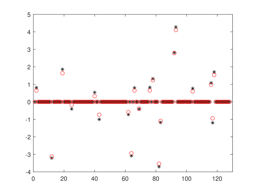
(a) RLNE $=6.17e-2$

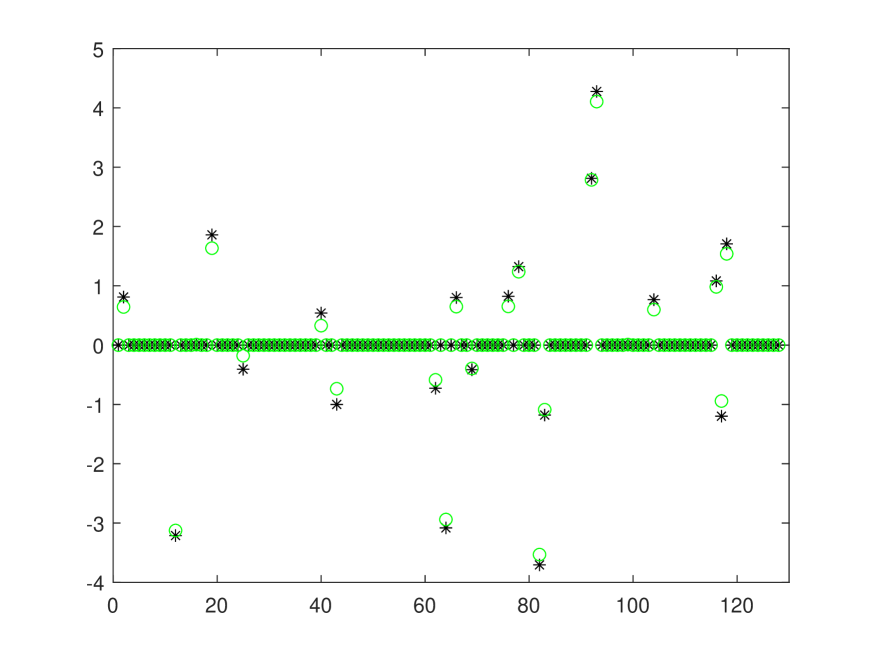
(b) RLNE $=6.17e-2$

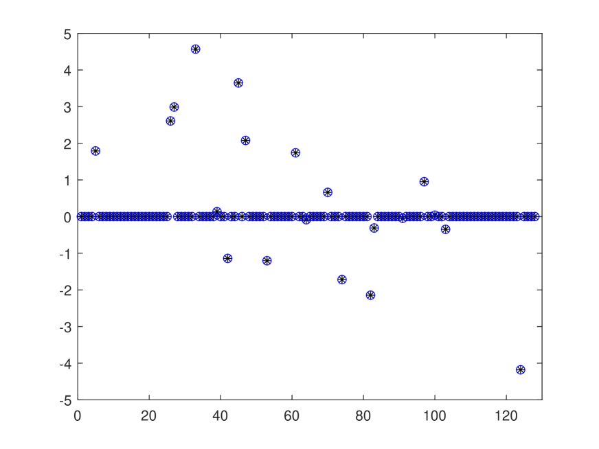
(c) RLNE $=8.47e-8$

Figure 1: Log-normal noise: the original signal (black stars) versus the recovery signals by ADMM_$\ell_{1-2}$ (red circles), FB_$\ell_{1-2}$ (green circles), and by PMM_$\ell_{p}$-$\ell_{1-2}$ (blue circles).

(a) RLNE $=4.76e-2$

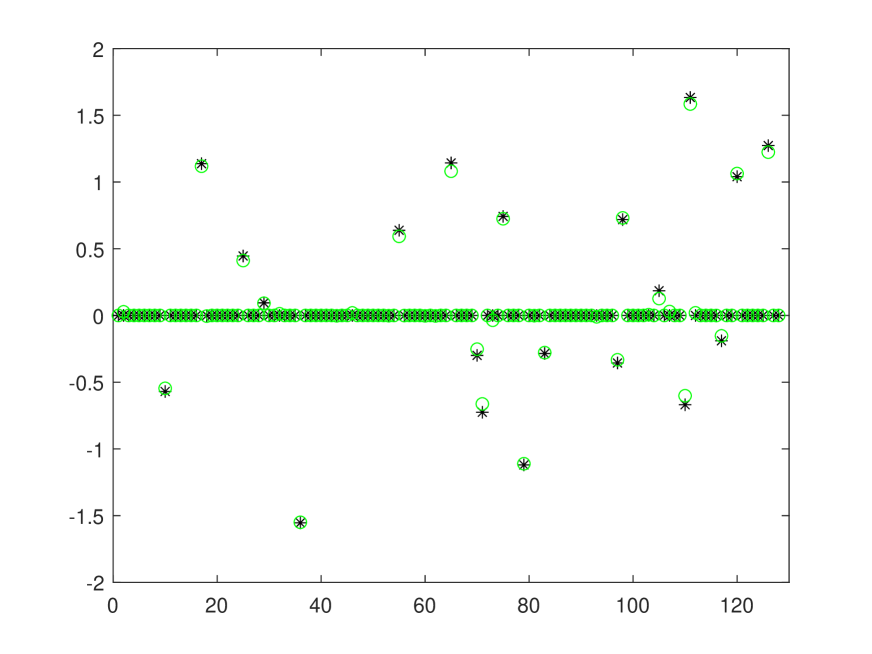
(b) RLNE $=4.76e-2$

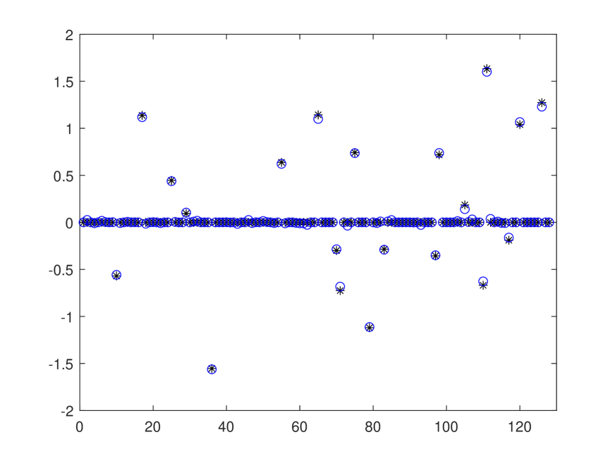
(c) RLNE $=3.92e-2$

Figure 2: Gaussian noise: the original signal (black stars) versus the recovery signals by ADMM_$\ell_{1-2}$ (red circles), FB_$\ell_{1-2}$ (green circles), and by PMM_$\ell_{p}$-$\ell_{1-2}$ (blue circles).

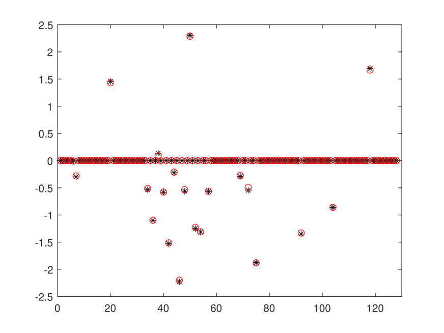
(a) RLNE $=1.92e-2$

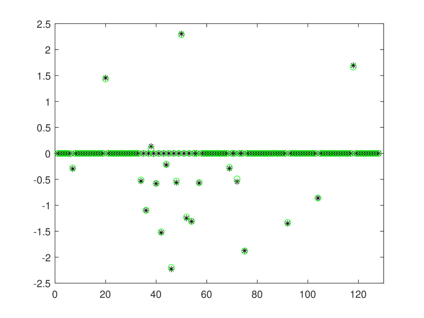
(b) RLNE $=1.92e-2$

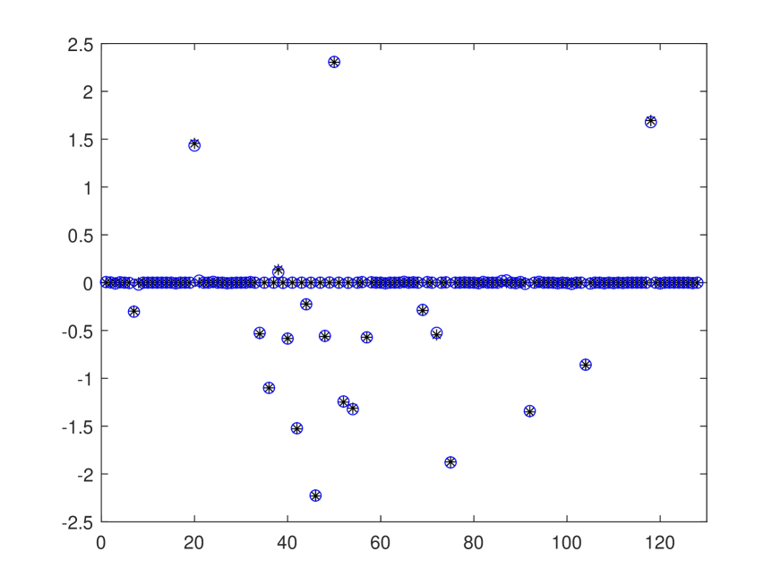
(c) RLNE $=1.37e-2$

Figure 3: Uniform noise: the original signal (black stars) versus the recovery signals by ADMM_$\ell_{1-2}$ (red circles), FB_$\ell_{1-2}$ (green circles), and by PMM_$\ell_{p}$-$\ell_{1-2}$ (blue circles).

In order to highlight the robustness and practicality of the model (1.2), we mainly test three different types of noises in this part. The observation $b$ is obtained by

$$b=A*\underline{x}+\alpha*\text{noise},$$

where $\alpha$ is the noise level, and “noise” is the one of the following types of noise: log-normal noise, Gaussian noise, and uniform noise. Here, we recover a sparse signal of being polluted by different kinds of noises via model (1.2) with different $p$ values. In this test, we set the noise level as $\alpha=1e-2$ and choose a random partial DCT to be a sensing matrix with size $64\times 128$. We say that the a signal $x$ is $K$-sparse if the number of nonzero entries in $x$ is $K$. In this test, we set $K=20$ to the ground truth signal $\underline{x}$. Finally, we also set $\beta\equiv 1$ for the sake of simplicity.

At the case of log-normal noise, we set $p=1$, i.e., the data fidelity term is $\|Ax-b\|_{1}$. Besides, the weighting parameter $\lambda$ in (1.2) is chosen as $\lambda=8e-2$. In Algorithm PMM_$\ell_{p}$-$\ell_{1-2}$, we let $\tau^{0}=1e-1$ and $\sigma^{0}=\sqrt{2}\|AA^{\top}\|_{2}$, and in algorithms ADMM_$\ell_{1-2}$ and FB_$\ell_{1-2}$, all the parameters are left to be their default settings. The original signal and the reconstructed signals recovered by PMM_$\ell_{p}$-$\ell_{1-2}$, ADMM_$\ell_{1-2}$, and FB_$\ell_{1-2}$ are listed respectively in Figure 1. In this figure, the original signal is denoted by black stars “$\ast$” and the recovered signals are denoted by “$\bigcirc$” marked in different color. Comparing each plot from left to right, we clearly see that all the stars in (c) are circled exactly by the blue circles with a symbol “$\circledast$” which indicates that the using of $\|Ax-b\|_{1}$ is better. Moreover, we also see that the final relative error of the solution derived by PMM_$\ell_{p}$-$\ell_{1-2}$ is $8.47e-8$ which is significantly smaller than the one produced by other algorithm, which once again indicates that the advantage of $\|Ax-b\|_{1}$. At the case of Gaussian noise, we set $p=2$ and $\tau^{0}=2$ , i.e., the data fidelity term is $\|Ax-b\|_{2}$, and at the case of uniform noise, we set $p=\infty$ and $\tau^{0}=1e-2$, i.e., the data fidelity term is $\|Ax-b\|_{\infty}$. Other parameters’ values in both cases are chosen as $\lambda=1e-2$ and $\sigma^{0}=\sqrt{2}\|AA^{\top}\|_{2}$. To be fair, we find that the two comparison algorithms perform better when $\lambda=1e-2$, so values of the parameters $\lambda=1e-2$ are fixed in ADMM_$\ell_{1-2}$ and FB_$\ell_{1-2}$ for $p=2,\infty$. The results of each algorithm for both different types of noise are listed in Figures 2 and 3, respectively. From these figures, we can visibly see that the quality of the solution derived by PMM_$\ell_{p}$-$\ell_{1-2}$ is better. From these limited numerical experiments, it can be concluded that, as far as the three types of noise are concerned, our proposed model (1.2) has the ability to get produce higher quality reconstruction results if the data fidelity term is chosen adaptively.

4.2..2 Test the superiority of $\ell_{1-2}$-term to $\ell_{1}$-norm under different sensing matrices and sparsity levels

In this section, we test the superiority of the $\ell_{1-2}$-term in two ways, i.e., using different sensing matrices and using different sparsity levels. To address the first issue, we test PMM_$\ell_{p}$-$\ell_{1-2}$, ADMM_$\ell_{1-2}$ and FB_$\ell_{1-2}$ repeatedly by the using of three types of sensing matrix, say random Gaussian matrix (GAUS), random partial DCT matrix (PDCT), and randomly oversampled partial DCT (ODCT). At each tested case, we run each algorithm based on two types of sparsity. All the parameters’ values are taken as the same as the ones previously except for the noise level $\alpha=1e-3$ and the weighting parameter $\beta$. In this test, the case of $\beta\equiv 0$ means that only a $\ell_{1}$-norm is used. The results of each algorithm with respect to the final relative error are listed in Table 1. From Table 1, we see that the RLNE values at the last column are always smaller than the corresponding ones at other two columns, which once again shows that our proposed model (1.2) indeed benefits the quality of the reconstruction solutions. Observing the results row-by-row, we find that, at most cases, the values at the case of $\beta=1$ are relatively smaller, which indicates that the “$-\|\cdot\|_{2}$”-term has the potential ability to extract sparse property.

Table 1: Final RLNE values of each algorithm

Sensing matrix	Dimension	Sparsity	$\beta$	ADMM_$\ell_{1-2}$	FB_$\ell_{1-2}$	PMM_$\ell_{p}$-$\ell_{1-2}$
GAUS	$50\times 100$	5	0	2.03e-2	2.03e-2	4.80e-3
	$50\times 100$	5	1	2.01e-2	2.01e-2	5.30e-3
	$400\times 800$	20	0	2.17e-2	2.17e-2	6.40e-3
	$400\times 800$	20	1	2.04e-2	2.04e-2	6.10e-3
PDCT	$50\times 100$	5	0	3.54e-2	3.54e-2	8.00e-3
	$50\times 100$	5	1	1.56e-2	1.56e-2	5.40e-3
	$400\times 800$	20	0	2.19e-2	2.19e-2	6.30e-3
	$400\times 800$	20	1	1.94e-2	1.94e-2	6.20e-3
ODCT (t=10)	$100\times 200$	5	0	5.22e-1	4.48e-1	4.39e-2
	$100\times 200$	5	1	1.08e-1	1.08e-1	1.64e-2
	$400\times 800$	10	0	7.40e-1	7.41e-1	3.08e-2
	$400\times 800$	10	1	3.74e-1	3.07e-1	1.51e-2
ODCT (t=15)	$100\times 200$	5	0	6.77e-1	6.08e-1	2.44e-1
	$100\times 200$	5	1	1.09e-1	1.09e-1	3.08e-2
	$400\times 800$	10	0	2.94e-1	2.30e-1	3.78e-1
	$400\times 800$	10	1	1.36e-1	1.36e-1	9.70e-3

We now turn our attention to using different sparsity levels to test the superiority of the $\ell_{1-2}$-term. In this test, the sensing matrices are chosen as the random Gaussian matrix with size $200\times 500$ and the randomly oversampled partial DCT matrix with $t=15$. For the sake of simplicity, we fix $\beta\equiv 1$ in the $\|x\|_{1}-\beta\|x\|_{2}$. Moreover, we also choose $\beta\equiv 0$ for comparison and the names of the corresponding algorithms are abbreviated as “$***\_{\ell_{1}}$”. The original signal $\underline{x}$ tested on random Gaussian matrix has a support size of $5:2:25$, which means that the support size starts from $5$ and ends at $25$ with an increment of $2$. The true signal $\underline{x}$ used at the randomly oversampled partial DCT matrix case has a support size of $5:1:15$. The statistical results on each tested case drawn in Figure 4.

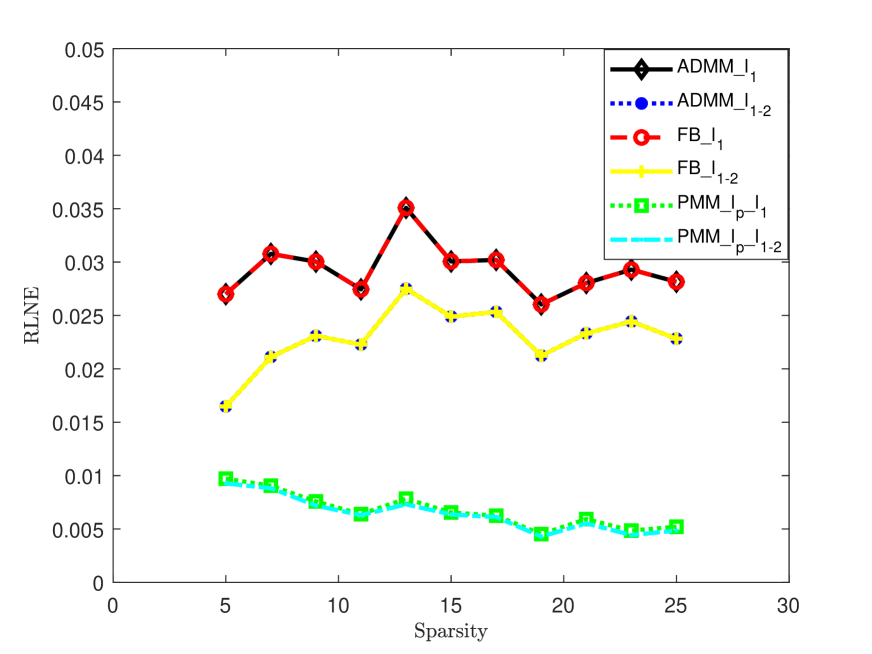
(a) Gaussian matrix

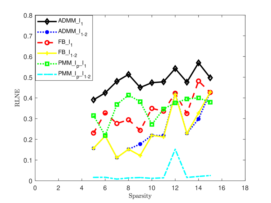
(b) ODCT matrix with $t=15$

Figure 4: RLNE values under different sparsity levels

As can be seen from left plot that, the curves derived by PMM_$\ell_{p}$-$\ell_{1}$ and PMM_$\ell_{p}$-$\ell_{1-2}$ are always at the bottom which show that our proposed approach is a winner. Moreover, we also see that the curves derived by “$***\_{\ell_{1}}$” and “$***\_{\ell_{1-2}}$” are almost the same, which indicates that the “$-\|\cdot\|_{2}$” term has hardly any influence at the random Gaussian matrix case. While we turn our attention to the right plot, it is easy to see that the curves derived by PMM_$\ell_{p}$-$\ell_{1}$ lie under the one by ADMM_$\ell_{1-2}$ and FB_$\ell_{1-2}$ which once again shows our proposed approach is better. However, at each test case, the curves derived by “$***\_{\ell_{1}}$” and “$***\_{\ell_{1-2}}$” are totally different, and the curves based on the “$-\|\cdot\|_{2}$” term are always at the bottom. From this phenomenon, we conclude that the “$-\|\cdot\|_{2}$” term is capable of improving the quality of the reconstruction solutions. Taking everything together, these experiments under different sensing matrices and different sparsity levels show that the superiority of the proposed model in recovering sparse signals is obvious.

4.3. Evaluate the Performance of PMM_$\ell_{p}$-$\ell_{1-2}$

In this part, we test PMM_$\ell_{p}$-$\ell_{1-2}$ against DCA_ADMM — a the difference of convex functions algorithm (DCA) in which the subproblem is solved by alternating direction method of multipliers. We firstly describe some implementation details of using ADMM to solve the second subproblem in (3.6). Denote $y:=Ax-b$. The subproblem of DCA exhibited in (3.6) can be written equivalently as

$$\begin{array}[]{lll}\min\limits_{x,y}&\|y\|_{p}+\lambda\|x\|_{1}-\lambda\beta\langle v^{k},x\rangle\\ \text{s.t.}&Ax-y=b.\\ \end{array}$$ (4.21)

Let $\sigma>0$ be a penalty parameter, the augmented Lagrangian function associated with problem (4.21) is given by

$$\mathcal{L}_{\sigma}(x,y;u) =\|y\|_{p}+\lambda\|x\|_{1}-\lambda\beta\langle v^{k},x\rangle+\langle u,Ax-y-b\rangle+\frac{\sigma}{2}\|Ax-y-b\|^{2}_{2},$$

where $u\in\mathbb{R}^{m}$ is a multiplier associated with the constraint. Staring from an initial point $(x^{0},y^{0};u^{0})$, the semi-proximal ADMM for solving (4.21) is summarized as

$$\left\{\begin{array}[]{l}y^{j+1}=\operatorname*{arg\,min}_{y}\big{\{}\|y\|_{p}+\frac{\sigma}{2}\|Ax^{j}-y-b+u^{j}/\sigma\|_{2}^{2}+\frac{\sigma}{2}\|y-y^{j}\|_{S}^{2}\big{\}},\\[8.53581pt] x^{j+1}=\operatorname*{arg\,min}_{x}\big{\{}\lambda\|x\|_{1}-\lambda\beta\langle v^{k},x\rangle+\frac{\sigma}{2}\|Ax-y^{j+1}-b+u^{j}/\sigma\|_{2}^{2}+\frac{\sigma}{2}\|x-x^{j}\|_{T}^{2}\big{\}},\\[8.53581pt] u^{j+1}=u^{j}+\tau\sigma\big{(}Ax^{j+1}-y^{j+1}-b\big{)},\end{array}\right.$$ (4.22)

where $S$ and $T$ are weighted positive semi-definite matrices, and $\tau$ is steplength chosen in the interval $(0,(1+\sqrt{5})/2)$. Choose $S:=0$ and $T:=\zeta I-{\mathcal{A}}^{\top}A$ where $\zeta>0$ be a positive scalar such that $T$ be positive semi-definite. It is a trivial task to deduce that the $y$- and $x$-subproblems can be written as the following proximal mapping forms

$$y^{j+1}=\operatorname{Prox}_{{\sigma}^{-1}\|\cdot\|_{p}}\Big{(}Ax^{j}-b+u^{j}/\sigma\Big{)},$$

and

$$x^{j+1}=\operatorname{Prox}_{(\zeta\sigma)^{-1}\lambda\|\cdot\|_{1}}\Big{(}\frac{A^{\top}[y^{j+1}+b-u^{j}/\sigma]+[\zeta I-A^{\top}A]x^{j}}{\zeta}+\frac{\lambda\beta v^{k}}{\zeta\sigma}\Big{)},$$

which means that the iterative scheme (4.22) is easily implementable in the sense that both subproblems admit explicit form solutions from Lemma 2.1. We must emphasize that the iterative framework (4.22) is actually an implementation of the semi-proximal ADMM of Fazel et al. Fazel et al. (2013). Hence, its convergence can be guaranteed under some technical conditions. For more details, one may refer to (Fazel et al., 2013, Theorem B).

We now compare the numerical performance of two different methods for solving problem (1.2). In this test, we set the noise level as $\alpha=1e-3$ and choose diverse sensing matrices and different sparsity. For Algorithm PMM_$\ell_{p}$-$\ell_{1-2}$, we set the same parameters as Section 4.2. For fairness, we take the same penalty parameter $\lambda$ and set $\beta=1$ in model (1.2) for both algorithms. In addition, the parameter ${\sigma}$ in DCA_ADMM and the initial $\sigma^{0}$ in PMM_$\ell_{p}$-$\ell_{1-2}$ are fixed as $\sqrt{2}\|AA^{\top}\|_{2}$. These settings always make both algorithms work well during the experiments’ preparations. For the $\ell_{p}$-norm in data fidelity term, we choose $p=1$ at the case of log-normal noise (LN), $p=2$ for Gaussian noise (GN), and $p=\infty$ for uniform noise (UN). Detailed numerical results are reported in Table 2 which contains the names of the noise types (Noise), the type of sensing matrix (Matrix) with its dimensions (Dim), the CPU time required in seconds (Time), the final objective function value of (1.2) (Obj), the values of RLNE and RelErr, and the number of outer iterations (Iter). Besides, the symbol “-” presents the algorithm failed to achieve convergence within $2000$ number of iterations.

Table 2: The performance of the PMM_$\ell_{p}$-$\ell_{1-2}$ and DCA_ADMM.

					PMM_$\ell_{p}$-$\ell_{1-2}$				DCA_ADMM
Noise	Matrix(Dim)	K	$\lambda$	$\sigma^{0}(\sigma)$	Time	Obj	RLNE	Iter	Time	Obj	RLNE	Iter
LN	GAUS($100\times 200$)	10	0.02	1	0.0541	0.4873	9.61e-9	15	0.0773	0.4873	3.64e-6	64
	GAUS($400\times 800$)	20	0.04	2	0.8318	0.8546	1.97e-10	14	1.3320	0.8546	3.65e-6	39
	PDCT($200\times 400$)	10	0.06	2	0.0515	1.3326	4.87e-10	5	0.1005	1.3326	9.38e-7	16
	PDCT($400\times 800)$	20	0.08	1.5	0.2232	2.1734	4.37e-10	5	0.5021	2.1734	7.00e-7	14
GN	GAUS($100\times 200$)	10	0.005	1	0.1499	0.0281	0.0110	20	0.1612	0.081	0.0110	20
	GAUS($400\times 800$)	20	0.015	2	4.1701	0.1795	0.0134	20	6.2627	0.1795	0.0144	16
	ODCT(t=5)($100\times 200$)	10	0.08	0.1	0.1225	0.4224	0.0067	8	3.0180	0.4724	0.0040	-
	ODCT(t=10)($200\times 400$)	15	0.05	0.3	3.0582	0.5294	0.0179	93	146.3076	0.5385	0.3085	-
UN	GAUS($64\times 128$)	10	0.005	2	2.7091	0.0244	0.0060	213	8.9643	1.7752	1.2280	-
	GAUS($128\times 256$)	15	0.001	2	6.1933	0.0084	0.0054	803	22.7704	2.5062	1.2862	-
	PDCT($64\times 128$)	10	0.01	2	0.4581	0.0378	0.0028	21	9.0736	2.2083	1.0323	-
	PDCT($128\times 256)$	15	0.005	2	2.3322	0.0531	0.0019	51	26.7144	42.7302	0.6863	-

At the fist place, we can clearly see that the final RLNE and objective function values are obviously smaller than DCA_ADMM at all the instances. On the one hand, we see that PMM_$\ell_{p}$-$\ell_{1-2}$ can successfully solve the problem all the instances to the desired accuracy within hundreds or even dozens of steps, while DCA_ADMM must be stopped when it reaches the maximum number of $2000$ iterations at some cases. On the other hand, we can observe that PMM_$\ell_{p}$-$\ell_{1-2}$ always takes much less time than DCA_ADMM. For example, for the instance GN with ODCT(t=5) matrix, we can see that PMM_$\ell_{p}$-$\ell_{1-2}$ is nearly $30$ times faster than DCA_ADMM. In addition, at the ODCT(t=10) sensing matrix case, PMM_$\ell_{p}$-$\ell_{1-2}$ can solve the instance within seconds while DCA_ADMM reaches the maximum of $20000$ iterations and consumes more than $2$ minuets but only produces a rather lower accuracy solution. Overall, we conclude that PMM_$\ell_{p}$-$\ell_{1-2}$ is clearly more robust and efficient than DCA_ADMM on the limited experiments.

5 Conclusions

The compressive sensing theories offered the possibilities to reconstruct a large and sparse signal from highly undersampled data and remove the possible noise simultaneously. However, the selection of the data fidelity type is known to be much noise depending. Besides, the efficiencies of almost all the reconstruction models depend heavily on the corresponding numerical algorithms. Hence, designing a flexible model along with an efficient algorithm which is capable of dealing with more types of noise is especially important. Using the difference between $\ell_{1}$-norm and $\ell_{2}$-norm as a regularization instead of using the $\ell_{1}$-norm alone has been numerically shown to be more efficiency to extract sparse property even under high coherent condition. While enjoying these advantages, at the same time, it also bring much difficulties because the “$\|x\|_{1}-\beta\|x\|_{2}$” term is nonsmooth and nonconvex, and the “$\|Ax-b\|_{p}$” term is nonsmooth. To address these issues, we used a proximal majorization technique to make the term “$-\|x\|_{2}$” be convex, and then employed a semismooth Newton method to solve the resulting semismooth equations. We must emphasize that the $x$- and $y$-subproblems in Step $4$ of Algorithm SSN admits analytical solutions if $p$ is chosen as $1$, $2$, or $\infty$, which indicates that the algorithm is easily implementable. Finally, we did a series of numerical experiments using different noise types, different sensing matrices, and different sparsity levels. The numerical results showed that the robustness of the proposed model are very evident and the performance of the proposed algorithm is very clear. Despite this, the Assumption 3.3 to ensure the positive definiteness of the generalized Jacobian $\tilde{\partial}^{2}\Theta(\bar{u})$ at the case of $p=\infty$ looks strong. Hence, some theoretical improvements to this issue is highly required. But this doesn’t affect us to believe that PMM_$\ell_{p}$-$\ell_{1-2}$ is a valid for sparse signal reconstructing and it may have its own extraordinary potency in other related problems. At last but not at least, to the best of our knowledge, PMM_$\ell_{p}$-$\ell_{1-2}$ is the first algorithm to solve (1.2), and hence, other efficient algorithms are worthy of designing.

References

- Bellec et al. (2018) Bellec, P. C., G. Lecue, and A. B. Tsybakov (2018). Slope meets lasso: improved oracle bounds and optimality. The Annals of Statistics 46, 3603–3642.
- Belloni and Chernozhukov (2011) Belloni, A. and V. Chernozhukov (2011). L1-penalized quantile regression in high-dimensional sparse models. The Annals of Statistics 39, 82–130.
- Belloni et al. (2011) Belloni, A., V. Chernozhukov, and L. Wang (2011). Square-root lasso: pivotal recovery of sparse signals via conic programming. Biometrika 98, 791–806.
- Candes and Tao (2005) Candes, E. J. and T. Tao (2005). Decoding by linear programming. IEEE Transactions on Information Theory 51, 4203–4215.
- Chen et al. (2014) Chen, X. J., D. D. Ge, Z. Z. Wang, and Y. Y. Ye (2014). Complexity of unconstrained - minimization. Mathematical Programming 143, 371–383.
- Chen et al. (2010) Chen, X. J., F. M. Xu, and Y. Y. Ye (2010). Lower bound theory of nonzero entries in solutions of - minimization. SIAM Journal on Scientific Computing 32, 2832–2852.
- Clarke (1983) Clarke, F. H. (1983). Optimization and Nonsmooth Analysis. Wiley, New York.
- Cui et al. (2018) Cui, Y., J. S. Pang, and B. Sen (2018). Composite difference-max programs for modern statistical estimation problems. SIAM Journal on Optimization 28, 3344–3374.
- Daubechies et al. (2009) Daubechies, I., R. DeVore, M. Fornasier, and C. Gunturk (2009). Iteratively reweighted least squares minimization for sparse recovery. Communications on Pure and Applied Mathematics 63, 1–38.
- Donoho (2006) Donoho, D. L. (2006). Compressed sensing. IEEE Transactions on Information Theory 52, 1289–1306.
- Donoho and Elad (2003) Donoho, D. L. and M. Elad (2003). Optimally sparse representation in general (nonorthogonal) dictionaries via minimization. Proceedings of the National Academy of Sciences of the United States of America 100, 2197–2202.
- Facchinei and Kanzow (1997) Facchinei, F. and C. Kanzow (1997). A nonsmooth inexact Newton method for the solution of large-scale nonlinear complementarity problems. Mathematical Programming 76, 4930–512.
- Fazel et al. (2013) Fazel, M., T. K. Pong, D. F. Sun, and P. Tseng (2013). Hankel matrix rank minimization with applications in system identification and realization. SIAM Journal on Matrix Analysis and Applications 34(3), 946–977.
- Gribonval and Nielsen (2003) Gribonval, R. and M. Nielsen (2003). Sparse representations in unions of bases. IEEE Transactions on Information Theory 49, 320–3325.
- Hiriart-Urruty and Lemarechal (2013) Hiriart-Urruty, J. B. and C. Lemarechal (2013). Convex Analysis and Minimization Algorithms I: Fundamentals. Springer Science Business Media.
- Kummer (1988) Kummer, B. (1988). Newton’s method for non-differentiable functions. Advances in Mathematical Optimization, 114–125.
- Lemarechal and Sagastizabal (1997) Lemarechal, C. and C. Sagastizabal (1997). Practical aspects of the Moreau-Yosida regularization: Theoretical preliminaries. SIAM Journal on Optimization 7, 367–385.
- Li et al. (2018) Li, X. D., D. F. Sun, and K.-C. Toh (2018). A highly efficient semismooth Newton augmented Lagrangian method for solving Lasso problems. SIAM Journal on Optimization 28, 433–458.
- Lin et al. (2020) Lin, M. X., D. F. Sun, and K.-C. Toh (2020). Efficient algorithms for multivariate shape-constrained convex regression problems. https://arxiv.org/pdf/2002.11410.pdf.
- Lou et al. (2015) Lou, Y. F., S. Osher, and J. Xin (2015). Computational aspects of L1-L2 minimization for compressive sensing. Advances in Intelligent Systems Computing 359, 169–180.
- Lou and Yan (2018) Lou, Y. F. and M. Yan (2018). Fast L1-L2 minimization via a proximal operator. Journal of Scientific Computing 74, 767–785.
- Lou et al. (2015) Lou, Y. F., P. H. Yin, Q. He, and J. Xin (2015). Computing sparse representation in a highly coherent dictionary based on difference of L1 and L2. Journal of Scientific Computing 64, 178–196.
- Lu (2014) Lu, Z. S. (2014). Iterative reweighted minimization methods for regularized unconstrained nonlinear programming. Mathematical Programming 147, 277–307.
- Martinez and Qi (1995) Martinez, J. M. and L. Q. Qi (1995). Inexact Newton methods for solving nonsmooth equations. Journal of Computational and Applied Mathematics 60, 127–145.
- Mifflin (1977) Mifflin, R. (1977). Semismooth and semiconvex functions in constrained optimization. SIAM Journal on Control and Optimization 15, 959–972.
- Moreau (1964) Moreau, J. J. (1964). Proximité et dualité dans un espace hilbertien. Bulletin de la Société Mathématique de France 93, 273–299.
- Qi (1993) Qi, L. Q. (1993). Convergence analysis of some algorithms for solving nonsmooth equations. Mathematics of Operations Research 18, 227–244.
- Qi and Sun (1993) Qi, L. Q. and J. Sun (1993). A nonsmooth version of Newton’s method. Mathematical programming 58, 353–367.
- Rockafellar (1970) Rockafellar, R. T. (1970). Convex Analysis. Princeton University Press.
- Rockafellar and Wets (1998) Rockafellar, R. T. and R. J.-B. Wets (1998). Variational Analysis. Springer, New York.
- Tang et al. (2020) Tang, P. P., C. J. Wang, D. F. Sun, and K.-C. Toh (2020). A sparse semismooth Newton based proximal majorization-minimization algorithm for nonconvex square-root-loss regression problems. Journal of Machine Learning Research 21, 1–38.
- Wang (2013) Wang, L. (2013). penalized LAD estimator for high dimensional linear regression. Journal of Multivariate Analysis 120, 135–151.
- Wen et al. (2018) Wen, Y. W., W. K. Ching, and M. Ng (2018). A Semi-smooth Newton Method for Inverse Problem with Uniform Noise. Journal of Scientific Computing 75, 713–732.
- Xiu et al. (2018) Xiu, X. C., L. C. Kong, Y. Li, and H. D. Qi (2018). Iterative reweighted methods for minimization. Computational Optimization and Applications 70, 201–219.
- Xue et al. (2019) Xue, Y. H., Y. F. Feng, and C. L. Wu (2019). An efficient and globally convergent algorithm for - model in group sparse optimization. Communications in Mathematical Sciences 18, 227–258.
- Yin et al. (2015) Yin, P. H., Y. F. Lou, Q. He, and J. Xin (2015). Minimization of for compressed sensing. SIAM Journal on Scientific Computing 37, A536–A563.
- Yosida (1964) Yosida, K. (1964). Functional Analysis. Springer, Berlin.
- Zhang and Wei (2015) Zhang, Z. and W. Y. Wei (2015). Primal-Dual approach for uniform noise removal. First International Conference on Information Science and Electronic Technology (ISET 2015).