A Unified Decision Framework for Phase I Dose-Finding Designs

Abstract

The purpose of a phase I dose-finding clinical trial is to investigate the toxicity profiles of various doses for a new drug and identify the maximum tolerated dose. Over the past three decades, various dose-finding designs have been proposed and discussed, including conventional model-based designs, new model-based designs using toxicity probability intervals, and rule-based designs. We present a simple decision framework that can generate several popular designs as special cases. We show that these designs share common elements under the framework, such as the same likelihood function, the use of loss functions, and the nature of the optimal decisions as Bayes rules. They differ mostly in the choice of the prior distributions. We present theoretical results on the decision framework and its link to specific and popular designs like mTPI, BOIN, and CRM. These results provide useful insights into the designs and their underlying assumptions, and convey information to help practitioners select an appropriate design.

1 Introduction

We construct a Bayesian decision theoretic framework for dose finding trials and show how several popular designs can be derived as special cases. Understanding many designs as special cases of one common general construction helps investigators to put a rapidly increasing number of seemingly competing alternative designs into perspective and to appreciate the relative strengths and limitations of different algorithms. A phase I clinical trial is the first stage of in-human investigation of a new drug or therapy. Phase I dose-finding designs aim to identify the maximum tolerate dose (MTD) and to provide dose recommendation for later phase trials. In the vast majority of phase I trials, a set of ascending candidate doses is tested for toxicity and the dose toxicity probability is assumed to be monotonically increasing with the dose level. Typically, the MTD is defined as the highest dose with a dose limiting toxicity (DLT) probability closest to, or not higher than a target toxicity probability $p_{T}$. Usually $p_{T}$ ranges from $0.17$ and $0.3$. In addition, some designs include the notion of an equivalence interval (EI) to allow for variations in the definition of the MTD. For example, one may choose to set $p_{T}=0.3$ and EI $=(p_{T}-\epsilon_{1},p_{T}+\epsilon_{2})=(0.25,0.35)$. This means that the target DLT probability of the MTD is 0.3, but doses with DLT probabilities between 0.25 and 0.35 can also be considered as the MTD. In other words, the EI allows investigators to consider doses with toxicity probabilities within the EI interval as appropriate MTD candidates.

A variety of statistical designs for phase I dose-finding trials has been discussed in the literature. A design consecutively assigns patients to recommended dose levels based on the observed DLT outcomes from previously enrolled patients. Existing designs can broadly be divided into two categories, rule-based designs and model-based designs. Among model-based designs, some use simple models and are sometimes called “model-assisted” designs. See Figure 1 for an illustration. We provide a brief introduction of the designs in Figure 1 next.

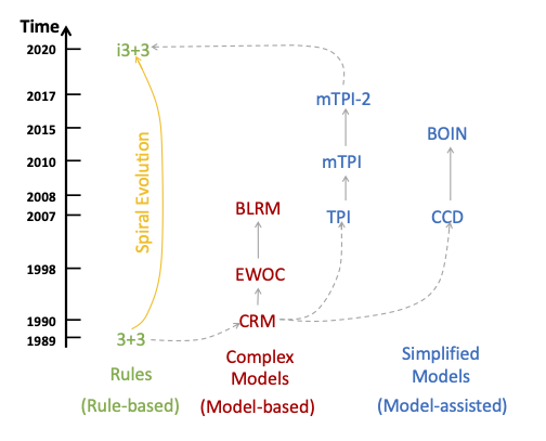
Figure 1: Illustration of some Phase I designs. Dotted lines connect designs across different categories, and solid lines connect designs within the same category. Arrows represents the sequence of original publication dates.

The 3+3 design [16] is rule-based and consecutively assigns patients to the current dose or the adjacent higher or lower doses based on observed DLT outcomes. For example, if the current dose at which patients are assigned is $d$, then 3+3 assigns the next patient cohort to doses $(d+1)$, $(d-1)$, or $d$ itself. This is called the “up-and-down” rule. Based on the same up-and-down rule, a smarter rule-based design, i3+3, is proposed in Liu et al. [12] by accounting for higher sampling variability when the sample size at a dose is small. The i3+3 design maintains simplicity of rule-based designs, and exhibits operating characteristics comparable to more complex model-based/assisted designs.

The continual reassessment method (CRM) [15], as the first model-based design in the literature, is based on an inference model with a parsimoniously parameterized dose-response curve. During the trial, CRM continuously updates the estimated dose-response curve based on the observed DLT data throughout the trial. CRM has motivated subsequent important work on model-based designs, including the Bayesian logistic regression method (BLRM) in Neuenschwander et al. [14] and the escalation with over-dose control (EWOC) in Tighiouart and Rogatko [18], among many others, all leveraging parametric dose-response models for statistical inference.

Recently, a class of designs, collectively known as “interval-based designs” take advantage of the notion of an EI to simplify statistical modeling and decision making for phase I trials. Notable examples include the toxicity probability interval (TPI) design [9] and its two modifications, mTPI [10], mTPI-2 [5] (equivalently, Keyboard [19]), the cumulative cohort (CCD) design [7], and the Bayesian optimal interval (BOIN) design [13]. These designs use simple models such as the beta/binomial hierarchical model and assume independence across dose toxicity probabilities, without attempting to explicitly model a dose-response curve. While the independence model assumption is apparently not true because dose toxicity is assumed to be monotonically increasing, it does not affect the operating characteristics of the interval-based designs due to various reasons like the safety restrictions in practice (e.g., no skipping in dose escalation). As a result, interval-based designs show robust performance based on simple up-and-down rules, restricting dosing decisions to be no more than one dose-level change from the current dose used in the trial. In other words, a simple independent beta/binomial model coupled with a simple up-and-down rule leads to desirable simulation performance that justifies the application of these designs. Importantly, the interval-based designs often generate a decision table that greatly simplifies the trial conduct and allow investigators to easily execute the dosing decisions provided in the table.

In the past three decades, many designs (CRM, mTPI, mTPI-2, BOIN, etc.) have been successfully applied to real-world trials. It is natural to wonder which design or designs are suitable for a particular trial. Recent reviews [20] and [6] provide some assessment of these designs, mainly from the perspective of simulation performance. Occasionally, conflicting conclusions might arise from different reviews based on the criteria used for design evaluation, or from different scenarios considered in the comparison. While simulation results can provide important information on the numerical performance of the designs, we argue that a theoretical investigation would complement the simulation results. In this article, we show that using the same optimal decision rule under the proposed decision framework, one can generate several published designs as special cases. In other words, we show a theoretical connection across different designs. These designs include mTPI, mTPI-2, BOIN, and CCD. In addition, based on the proposed decision framework, we develop a new version of the CRM design, called Int-CRM, that is founded on the same model assumption with the original CRM design but a different decision rule. We show that Int-CRM achieves comparable simulation performance as the original CRM design and other interval-based designs. The general decision framework provides insight into the similarities and differences across various designs and may assist investigators to select the right design for their specific needs.

The remainder of the paper is structured as follows. In Section 2, we introduce the unified decision framework and its main components. Section 3 shows how known designs fit into this framework, including the mTPI, mTPI-2, BOIN, CCD, and Int-CRM designs. In Section 4, we conduct simulation studies to assess the operating characteristics of the designs using the i3+3 and CRM designs as benchmarks. Finally, we conclude and end the paper with a discussion in Section 5.

2 Decision Framework

2.1 Overview

We cast the problem of dose finding as an optimization in a decision problem. In particular we focus on the myopic decision problem of selecting the dose for the next patient (cohort). It is myopic because the problem does not address the global decision of stopping the trial and dose selection; instead, the problem only considers the local optimal decision of finding the next dose for future patients. The main components of the decision framework have been briefly illustrated in Guo et al. [5] for the mTPI and mTPI-2 designs. A decision problem is characterized by an action space for decisions $a$, a probability model for all unknown quantities, and a loss function [1]. Table 1 shows a summary of these components.

Table 1: Components of the proposed decision framework.

Component	Notation	Notes
Probability model	$f(\bm{y}\mid\bm{\theta})\pi(\bm{\theta}\mid m)\pi(m)$	A hierarchical model with parameters $\bm{\theta}$ and $m$.
Action	$a$	Up-and-down dosing decisions, including
		$D$ (de-escalate), $S$ (stay), and $E$ (escalate).
Loss function	$\ell(a,\bm{\theta})$	The loss for taking action $a$
		where $\theta$ is the true parameter.
Optimal rule	$\mathcal{R}=\arg\min_{a}\int\ell(a,\bm{\theta})p(\bm{\theta}\mid\bm{y})d\bm{\theta}$	Bayes’ rule that chooses the action
		with the minimal posterior expected loss.

2.2 General Framework

In dose-finding trials with binary DLT endpoints, the parameter of interest is a set of toxicity probabilities, $\bm{\theta}=(p_{1},...,p_{T})$ at dose levels $x_{d}$, $d=1,\ldots,T$, where $T$ is the number of dose levels, and $p_{d}$ is the toxicity probability at dose $d$. Let $y_{d}$ denote the number of patients who experience DLTs out of $n_{d}$ patients treated at dose $d$, and let $\bm{y}=(y_{1},...,y_{T})$. For all methods in the upcoming discussion the sampling model $f(\bm{y}\mid\bm{\theta})$ in Table 1 is a binomial distribution with parameter $p_{d}$, i.e.,

$$y_{d}\mid p_{d}\sim\mbox{Bin}(n_{d},p_{d}),\;\;\;d=1,...,T,$$

implying a likelihood function,

$$f(\bm{y}\mid\bm{\theta})\propto\prod_{d=1}^{T}p_{d}^{y_{d}}(1-p_{d})^{n_{d}-y_{d}}.$$

For model-based designs with a dose-response curve, toxicity probabilities are modeled as a function of the dose levels $x_{d}$. For example, a version of the CRM assumes $p_{d}=q_{d}^{exp(\alpha)}$, and a single parameter $\theta=\alpha$ (the values $q_{d}$ are fixed and are known as the “skeleton”). The BLRM design uses $p_{d}=logit^{-1}(\alpha+\beta x_{d})$ with parameters $\bm{\theta}=(\alpha,\beta)$.

The proposed decision framework uses a concept of probability intervals. The parameter of interest is $p_{d}$, and the parameter space of $p_{d}$ is $I=[0,1]$. Consider a set of intervals within $I$, denoted as $\Omega=\{I_{k},\;k=1,...,K\}$, which form a partition of the parameter space $I$. That is, $\bigcup_{k=1}^{K}I_{k}=I$ and $I_{k}\cap I_{k^{\prime}}=\emptyset,\;\;k\neq k^{\prime}$. The true value of $p_{d}$ belongs to one and only one of the intervals. For example, $\Omega=\{I_{1}=[0,0.5],I_{2}=(0.5,1]\}$ is a partition, and if $p_{d}=0.3$, $p_{d}\in I_{1}$. We introduce a latent indicator $m_{d}$ (or, for short, just $m$) with $m_{d}=k$ if $p_{d}\in I_{k}$, and define a hierarchical model prior $\pi(m)$ and $\pi(p_{d}\mid m)$. For example, $\pi(m=k)=\frac{1}{K},\;\;\;k=1,...,K,$ and $\pi(\bm{\theta}\mid m=k)\propto\prod_{d=1}^{T}\mbox{Be}(\alpha,\beta)\delta(p_{d}\in I_{k}),$ a truncated beta distribution. Here, $\delta(\cdot)$ is an indicator function. That is, $p_{d}$ are conditionally independent with pdf

$$p(p_{d}\mid m=k)=\frac{beta(p_{d};\alpha,\beta)\delta(p_{d}\in I_{k})}{\int_{I_{k}}beta(p_{d};\alpha,\beta)dp_{d}},$$

where $beta(p_{d};\alpha,\beta)=\frac{\Gamma(\alpha+\beta)}{\Gamma(\alpha)\Gamma(\beta)}p_{d}^{\alpha-1}(1-p_{d})^{\beta-1},\alpha>0,\beta>0$ is a $\mbox{Be}(\alpha,\beta)$ p.d.f.

We consider a special partition $\Omega=\{I_{1},I_{2},I_{3}\}$ where $I_{2}=I_{S}=EI=(p_{T}-\epsilon_{1},p_{T}+\epsilon_{2})$, $I_{1}=I_{E}=[0,p_{T}-\epsilon_{1}]$, and $I_{3}=I_{D}=[p_{T}+\epsilon_{2},1]$. Therefore, $K=3$ and we use notations $I_{S}$, $I_{E}$, and $I_{D}$ to associate the intervals with corresponding up-and-down dose-finding decisions S, E, and D, respectively. We summarize the proposed decision framework below.

Likelihood

$$f(\bm{y}\mid\bm{\theta})\propto\prod_{d=1}^{D}p_{d}^{y_{d}}(1-p_{d})^{n_{d}-y_{d}},$$ (1)

where $p_{d}$ is the toxicity probability for dose $d$, $d=1,\dots,D$.

Prior

We assume $p_{d}$ are a priori independent and

$$\pi(p_{d}\mid m=k) \propto g(p_{d})\delta(p_{d}\in I_{k}),\;\;\;k=1,...,K,$$

$$\pi(m=k) = \frac{1}{K},\;\;\;k=1,...,K.$$

For example, $g(p_{d})=beta(p_{d};\alpha,\beta)$.

Partition

$\Omega=\{I_{E}(I_{1}),\;I_{S}(I_{2}),\;I_{D}(I_{3})\}$, where $I_{E}=[0,p_{T}-\epsilon_{1}],I_{S}=(p_{T}-\epsilon_{1},p_{T}+\epsilon_{2})$, and $I_{D}=[p_{T}+\epsilon_{2},1]$, and $I_{1}=I_{E}$, $I_{2}=I_{S}$, and $I_{3}=I_{D}$.

Actions

The actions are the three up-and-down decisions for dose-finding, i.e.,

$$a\in\mathcal{A}=\{E,S,D\},$$

where $\mathcal{A}$ denotes the action space. Here $E$, $S$, $D$ denote the dosing decisions “Escalation”, “Stay”, and “De-escalation,” respectively. In particular, if the last patient was assigned dose $d$, then $E$, $S$, or $D$ means treating future patients at dose $(d+1)$, $d$, or $(d-1)$, respectively.

Loss

We proceed with a myopic perspective, focusing on the decision for the respective next patient (cohort), and therefore specify a loss function for the next dose assignment $a$ only.

We use a 0-1 loss function,

$$\ell(a,p_{d})=\left\{\begin{array}[]{ll}1,&p_{d}\notin I_{a}\\ 0,&p_{d}\in I_{a}\end{array}\right.,\;\;\;\;a\in\mathcal{A}=\{E,S,D\}.$$ (4)

In words, when the action corresponds to an interval which contains the true parameter, the loss takes the value 0; otherwise, the loss equals 1. The loss function $\ell(a,p_{d})$ is stated in Table 2.

Table 2: The 0-1 loss function $\ell(a,\theta)$.

	$p_{d}\in$
$\ell(a,p_{d})$	$[0,p_{T}-\epsilon_{1}]$	$(p_{T}-\epsilon_{1},p_{T}+\epsilon_{2})$	$[p_{T}+\epsilon_{2},1]$
a = $D$	1	1	0
a = $S$	1	0	1
a = $E$	0	1	1

In other words, the loss function $\ell(a,p_{d})$ defines a 0-1 estimation loss for $m$, i.e., the interval that contains $p_{d}$.

Two more comments about the loss function and the setup of the decision problem. First, in general a loss (or, equivalently, utility) function could also be an argument of the outcome $y_{d}$. This is relevant, for example, if instead of inference loss we focus on the patients’ preferences. However, the intention of this discussion is only to highlight common structure in existing dose finding methods, for which we only need this restricted inference loss. Another important limitation is the myopic nature of the setup. We consider the dose allocation for each patient (or patient cohort) in isolation, ignoring that dose allocation now might help later decisions. That is, we ignore the sequential nature of the problem. Again, for the upcoming exposition of common underlying structure for the considered dose finding methods we will only refer to this myopic decision problem.

Bayes’ rule

The optimal decision rule for dose $d$ is the Bayes’ rule, defined as

$$\mathcal{R}_{d}=\arg\min_{a\in\mathcal{A}}\int\ell(a,p_{d})p(p_{d}\mid\bm{y})dp_{d},$$ (5)

which minimizes the posterior expected loss. Here, $p(p_{d}\mid\bm{y})$ is the posterior distribution of $p_{d}$.

In general, under a 0-1 estimation loss for a discrete parameter the Bayes rule is simply the posterior mode. The following result states this in the context of our problem. The Bayes’ rule is equivalent to the result of finding the interval with the maximal posterior probability.

Proposition 1

Denote $\Omega=\{I_{1},I_{2},I_{3}\}=\{I_{E},I_{S},I_{D}\}$, where $I_{1}=I_{E}$, $I_{2}=I_{S}$, $I_{3}=I_{D}$. Suppose dose $d$ is the current dose. Let $\{m=k\}$ denote the event $\{p_{d}\in I_{k}\},\;k\in\{1,2,3\}$. Let $\mathcal{A}=\{E,S,D\}$. Assume $\pi(m=k)=\frac{1}{3},\;k\in\{1,2,3\}$. The Bayes’ rule under the 0-1 loss in Equation (4) is given by

$$\mathcal{R}_{d} = \arg\max_{a\in\mathcal{A}}Pr(p_{d}\in I_{a}\mid\bm{y})$$

$$= \arg\max_{k\in\{1,2,3\}}Pr(m=k\mid\bm{y})$$

See Appendix C for a proof.

3 Design Examples

We show how various designs fit as special cases into this framework. That is, we provide examples of the decision framework that give rise to well-known designs including mTPI, BOIN, CCD, mTPI-2, and a new version of CRM, called the Int-CRM design.

3.1 Interval-based designs

We first introduce the connection between the decision framework and the interval-based designs, mTPI, mTPI-2, BOIN and CCD. These designs share some common components under the framework, but also include some elements specific to each design.

Common components

Likelihood (1), prior $\pi(m)$, loss function (4), and the nature of the defined dose allocation as Bayes’ rule.

Individual components

Prior $\pi(p_{d}\mid m)$, the specific partition $\Omega=\{I_{k},\;k=1,...,K\},$ and the definition of the action set $\mathcal{A}$.

All four interval-based designs use the binomial sampling model (1). And the designs share the same discrete uniform prior $\pi(m)$, the 0-1 loss function and the use of Bayes’ rule to select a decision. They divide the $[0,1]$ parameter space of $p_{d}$ into different intervals and use different priors. See Table 3 as a summary. We discuss details for each design next.

Table 3: Individual components of the proposed decision framework for some interval-based designs.

	mTPI	mTPI-2	BOIN/CCD
Actions	$\mathcal{A}=\{E,S,D\}$	$\mathcal{A}=\{1,...,K\}$	$\mathcal{A}=\{E,S,D\}$
	$I_{E}=[0,p_{T}-\epsilon_{1}]$	$I_{E}=I_{E,1}\cup\cdots\cup I_{E,K_{1}}$	$I_{E}=[0,\phi_{E}]$
Intervals	$I_{S}=(p_{T}-\epsilon_{1},p_{T}+\epsilon_{2})$	$I_{S}=(p_{T}-\epsilon_{1},p_{T}+\epsilon_{2})$	$I_{S}=(\phi_{E},\phi_{D})$
	$I_{D}=[p_{T}+\epsilon_{2},1]$	$I_{D}=I_{D,1}\cup\cdots\cup I_{D,K_{2}}$	$I_{D}=[\phi_{D},1]$
Priors	$\pi(p_{d}\mid m=k)\propto$	$\pi(p_{d}\mid m=k)\propto$	$\pi(p_{d}\mid m=k)=$
	$Be(1,1)\delta(p_{d}\in I_{k})$	$Be(1,1)\delta(p_{d}\in I_{k})$	$\delta(p_{d}=\phi_{k})$
1See Theorem 1 for details.

The mTPI design

For the mTPI design, given the equivalence interval EI$=(p_{T}-\epsilon_{1},p_{T}+\epsilon_{2})$, the $[0,1]$ parameter space is naturally partitioned into three intervals $\Omega=\{I_{1}=I_{E}=[0,p_{T}-\epsilon_{1}],I_{2}=I_{S}=(p_{T}-\epsilon_{1},p_{T}+\epsilon_{2}),I_{3}=I_{D}=[p_{T}+\epsilon_{2},1]\}$ that correspond to the actions $\mathcal{A}=\{E,S,D\}$, as shown in Table 3. The mTPI decision is equivalent to the Bayes’ rule $\mathcal{R}_{d}$ under the decision framework. See Corollary 1 below for a formal mathematical description.

Corollary 1.

The mTPI decision in Ji et al. [10] is given by

$$R_{mTPI}=\arg\max_{a\in\{E,S,D\}}\mbox{UPM}(I_{a}),$$

where UPM stands for “unit probability mass” and $\mbox{UPM}(I_{a})=Pr^{*}(p_{d}\in I_{a})/||I_{a}||$; here $||I_{a}||$ is the length of $I_{a}$, and $Pr^{*}(p_{d}\in I_{a})= \int B(y_{d}+1,n_{d}-y_{d}+1)\cdot p_{d}^{y_{d}}(1-p_{d})^{n_{d}-y_{d}}\cdot\delta(p_{d}\in I_{a})dp_{d}$ is calculated based on $p_{d}\sim\mbox{Be}(y_{d}+1,n_{d}-y_{d}+1)$. Let $I_{1}=I_{E}=[0,p_{T}-\epsilon_{1}]$, $I_{2}=I_{S}=(p_{T}-\epsilon_{1},p_{T}+\epsilon_{2})$, and $I_{3}=I_{D}=[p_{T}+\epsilon_{2},1]$. Then $R_{mTPI}=\mathcal{R}_{d}$, the Bayes rule under

$$\pi(p_{d}\mid m=k)=C_{k}\cdot beta(p_{d};1,1)\delta(p_{d}\in I_{k}),$$

where $beta(\cdot;1,1)$ denotes the density function of $\mbox{Be}(1,1)$ distribution and $C_{k}=\frac{1}{\int_{I_{k}}beta(p;1,1)dp}$ is a normalizing constant.

See Appendix C for a proof.

The mTPI-2 design

Ockham’s razor is a principle in statistical inference calling for an explanation of the facts to be no more complicated than necessary [17, 8]. In the context of model selection, the Ockham’s razor prefers parsimonious models that describe the data equally well as more complex models. In the proposed decision framework, $\{m=k\},\;k=1,...,K$, is equivalent to $K$ models $\{M_{k}:m=k\}$, and choosing the value of $m$ is equivalent to a model selection problem. Bayesian model selection chooses the model with the largest posterior probability (compare Proposition 1), i.e., $Pr(m=k\mid y)$, and models are automatically penalized for their complexity. In other words, Bayes’ rule $\mathcal{R}_{d}=\arg\max_{k\in\{1,2,3\}}Pr(m=k\mid y)$ implements Ockham’s razor if we define model complexity as $||I_{k}||$. Therefore, when the three models are $I_{1}=I_{E}=[0,p_{T}-\epsilon_{1}]$, $I_{2}=I_{S}=(p_{T}-\epsilon_{1},p_{T}+\epsilon_{2})$, $I_{3}=I_{D}=[p_{T}+\epsilon_{2}]$, the “simplest” model is $I_{2}=I_{S}$, since $\epsilon_{1}$ and $\epsilon_{2}$ are typically small probabilities ($\leq 0.05$).

Guo et al. [5] explain mTPI-2 as aiming to blunt Ockham’s razor by redefining a (finer) partition $\Omega^{*}=\{I_{E}^{*},I_{S}=EI,I_{D}^{*}\},$ where $I_{E}^{*}=\{I_{E,1},...,I_{E,K_{1}}\}$ and $I_{D}^{*}=\{I_{D,1},...,I_{D,K_{2}}\}$. Probability intervals $\{I_{E,k}\}_{k=2}^{K_{1}}$ and $\{I_{D,k}\}_{k=2}^{K_{2}}$ have the same length as $I_{S}=EI$. Let $K=K_{1}+K_{2}+1.$ The selected model $m$ under the mTPI-2 design can then be shown to be Bayes’ rule $\mathcal{R}_{d}$, under an action set $\mathcal{A}_{m}=\{1,...,K\}$. Corollary 2 next summarizes the results.

Corollary 2.

Under mTPI-2, $\Omega^{*}=\{I_{E}^{*}=\{I_{E,1},\cdots,I_{E,K_{1}}\},I_{S}=(p_{T}-\epsilon_{1},p_{T}+\epsilon_{2}),I_{D}^{*}=\{I_{D,1},\cdots,I_{D,K_{2}}\}\}$, $\mathcal{A}_{m}=\{1,...,K\}$. Assume the prior on $p_{d}$ is conditionally independent and given by

$$\pi(p_{d}\mid m=k)=C_{k}\cdot beta(p_{d};1,1)\delta(p_{d}\in I_{k}).$$

Then Bayes’ rule is

$$\mathcal{R}_{d}=\arg\max_{m\in\mathcal{A}_{m}}Pr(m=k\mid y)=\arg\max_{m\in\mathcal{A}_{m}}\mbox{UPM}(I_{m}).$$

See Appendix C for a proof. Corollary 2 establishes the Bayes’ rule $\mathcal{R}_{d}$ as an action in $\mathcal{A}_{m}=\{1,...,K\}$. To see the connection to the dose-finding decision in mTPI-2, we refer to the next result.

Corollary 3.

Let

$$\mathcal{R}_{\mbox{mTPI-2}}=\left\{\begin{array}[]{ll}E,&\arg\max_{I_{m}}\mbox{UPM}(I_{m})\subset(0,p_{T}-\epsilon_{1}),\\ S,&\arg\max_{I_{m}}\mbox{UPM}(I_{m})=(p_{T}-\epsilon_{1},p_{T}+\epsilon_{2}),\\ D,&\arg\max_{I_{m}}\mbox{UPM}(I_{m})\subset(p_{T}+\epsilon_{2},1).\end{array}\right.$$

Then

$${\mathcal{R}_{\mbox{mTPI-2}}}=\left\{\begin{array}[]{ll}E,&I_{\mathcal{R}_{d}}\subset(0,p_{T}-\epsilon_{1}),\\ S,&I_{\mathcal{R}_{d}}=(p_{T}-\epsilon_{1},p_{T}+\epsilon_{2}),\\ D,&I_{\mathcal{R}_{d}}\subset(p_{T}+\epsilon_{2},1).\end{array}\right.$$

In other words, if $\mathcal{R}_{d}=m^{*}$, then $I_{m^{*}}$ is the interval with the largest UPM, for $m^{*}\in\mathcal{A}_{m}$. And if $I_{M^{*}}$ is below, equal to, or above the EI$=(p_{T}-\epsilon_{1},p_{T}+\epsilon_{2})$, the decision is $E$, $S$, or $D$, respectively. This is the same as the up-and-down rule in the mTPI-2 design in Guo et al. [5]. Proof of Corollary 3 is immediate and omitted.

The BOIN design

The BOIN design [13] uses a decision rule

$$R_{BOIN}=\left\{\begin{array}[]{ll}E,&\hat{p}_{d}\leq\lambda_{1},\\ S,&\lambda_{1}<\hat{p}_{d}<\lambda_{2},\\ D,&\hat{p}_{d}\geq\lambda_{2},\end{array}\right.$$

where $\hat{p}_{d}=\frac{y_{d}}{n_{d}}$, $\lambda_{1}=\xi(\phi_{E};\phi_{S}),\lambda_{2}=\xi(\phi_{D};\phi_{S}),$ and

$$\xi(\phi_{i};\phi_{j})=\frac{log\left(\frac{1-\phi_{i}}{1-\phi_{j}}\right)}{log\left(\frac{\phi_{j}(1-\phi_{i})}{\phi_{i}(1-\phi_{j})}\right)}.$$ (10)

In particular, $\phi_{S}=p_{T}$, $\phi_{E}(<p_{T})$ and $\phi_{D}(>p_{T})$ are pre-specified values. Here, $\phi_{E}$ and $\phi_{D}$ play a similar rule as $(p_{T}-\epsilon_{1})$ and $(p_{T}+\epsilon_{2})$ in the mTPI and mTPI-2 designs, which defines the boundaries of an initial equivalence interval elicited from clinicians. We show that the decision rule $R_{BOIN}$ is also a Bayes’ rule under the proposed decision framework next.

Theorem 1.

Assume $y_{d}\mid p_{d}\sim\mbox{Bin}(n_{d},p_{d})$, $\pi(p_{d}\mid m=k)=\delta(p_{d}=\phi_{k})$, for $k=1,2,3$, and $\phi_{1}=\phi_{E}$, $\phi_{2}=\phi_{S}=p_{T}$, and $\phi_{3}=\phi_{D}$. Under the 0-1 loss $\ell(a,p_{d})$ in Equation (4), the Bayes’ rule is equivalent to $R_{BOIN}$, i.e.,

$$\mathcal{R}_{d}=R_{BOIN}=\left\{\begin{array}[]{ll}E,&\hat{p}_{d}\leq\lambda_{1},\\ S,&\lambda_{1}<\hat{p}_{d}<\lambda_{2},\\ D,&\hat{p}_{d}\geq\lambda_{2},\end{array}\right.$$

where $\hat{p}_{d}=\frac{y_{d}}{n_{d}}$, $\lambda_{1}=\xi(\phi_{E};\phi_{S}),\lambda_{2}=\xi(\phi_{D};\phi_{S}),$ and $\xi$ is defined as in Equation (10)

See Appendix C for a proof. By Theorem 1 the BOIN design takes the form of the Bayes’ rule under the same decision framework using the 0-1 loss. BOIN uses a point-mass prior for $p_{d}$ on three values, $\phi_{E}$, $\phi_{S}$, $\phi_{D}$, while mTPI/mTPI-2 using truncated beta priors instead. Next, we show that the BOIN design is almost the same as the CCD design. This is easiest seen under the perspective of the proposed decision framework. The difference between the two designs are the locations of the point-mass priors.

The CCD design

The CCD design [7] compares $\hat{p}_{d}$ with $(p_{T}-\epsilon_{1})$ and $(p_{T}+\epsilon_{2})$, and uses the following up-and-down rule,

$$\mathcal{R}_{\mbox{CCD}} = \left\{\begin{array}[]{ll}E&\hat{p}_{d}\leq p_{T}-\epsilon_{1}\\ S&p_{T}-\epsilon_{1}<\hat{p}_{d}<p_{T}+\epsilon_{2}\\ D&\hat{p}_{d}\geq p_{T}+\epsilon_{2}\end{array}\right.$$

Corollary 4 shows that the decision of the CCD design is the same Bayes’ rule in the same framework as BOIN but with a different prior distribution.

Corollary 4.

The CCD decision $\mathcal{R}_{\mbox{CCD}}=\mathcal{R}_{d}$ with

$$\pi(p_{d}\mid m=k)=\delta(p_{d}=\phi^{\prime}_{k}),\;\;\;k=E,S,D,$$

where $\phi^{\prime}_{E}=\xi^{-1}(p_{T}-\epsilon_{1})$, $\phi^{\prime}_{D}=\xi^{-1}(p_{T}+\epsilon_{2})$, $\phi^{\prime}_{S}=\phi_{S}=p_{T}$, and $\xi(\phi)\equiv\xi(\phi,p_{T})$ in Equation (10).

See Appendix C for a proof.

Corollary 4 shows that BOIN and CCD are identical designs with the only difference being that BOIN uses a point-mass prior $\pi(p_{d}\mid m=k)=\delta(p_{d}=\phi_{k})$, whereas CCD uses $\pi(p_{d}\mid m=k)=\delta(p_{d}=\phi^{\prime}_{k})$.

The Int-CRM design

Using the same decision framework, we propose a variation of the CRM design, called Int-CRM. We assume the same parametric dose-response model as in the CRM design [15], with the probability of toxicity monotonically increasing with dose. Let $d_{i}$ denote the dose for the $i$th patient, $d_{i}\in\{1,...,T\}$, and $Y_{i}$ the binary indicator of DLT. The dose-response curve is assumed to be the power model as in the CRM,

$$F(d,\theta)=q_{d}^{exp(\theta)},$$

where $(q_{1},..,q_{T})$ (“skeleton”) are a priori pre-specified dose toxicity probabilities. Other sensible dose-response models, such as a logit model, may be considered as well. The toxicity rates are dependent across doses through the dose-response curve and the inference is based on the parameter $\theta$. The likelihood function is given by

$$f(\bm{y}\mid\theta)\propto\prod_{i=1}^{n}F(d_{i},\theta)^{y_{i}}\{1-F(d_{i},\theta)\}^{1-y_{i}},$$

where $n$ is the number of patients in the trial.

Following Cheung and Chappell [3], we define an interval $[A_{1},A_{T+1}]$ for $\theta$ that is wide enough to allow for a wide range of dose-response curves. For example, set $A_{1}$ and $A_{T+1}$ so that $q_{1}^{exp(A_{1})}>1-10^{-5}$ and $q_{T}^{exp(A_{T+1})}<10^{-5}$, which correspond to response curves constantly equal to 1.0 and 0.0, respectively, and $\theta\in[A_{1},A_{T+1}]$ allows choices in-between these extremes. Using $A_{1}$ and $A_{T+1}$, we define sub-intervals for $\theta$ as the set of values that imply $d_{k}$ having toxicity probability closest to $p_{T}$,

$$I_{k}=\{\theta\in[A_{1},A_{T+1}]:|F(k,\theta)-p_{T}|<|F(d,\theta)-p_{T}|,\forall d\neq k\},$$

k=1, …, T. As shown in Cheung and Chappell [3], $I_{k}$ is an interval, denoted as $I_{1}=[\psi_{1}=A_{1},\psi_{2})$, $I_{k}=[\psi_{k},\psi_{k+1}),\;k=2,...,(T-1)$, $I_{T}=[\psi_{T},\psi_{T+1}=A_{T+1}]$, where $\psi_{k}$ is implicitly defined as the solution of

$$F(k-1,\psi_{k})+F(k,\psi_{k})=2p_{T},\;\;\;k=2,...,T.$$

Given the “skeleton” $(q_{1},...,q_{T})$, we can obtain the numerical result of the interval boundaries $\phi_{k}$’s by solving the equation above. See Appendix B for details. Each interval consists of a set of $\theta$ values where dose $k$’s toxicity probability is the closest to $p_{T}$ among all the doses. We use these intervals $I_{k}$’s in our framework for Int-CRM. We propose hierarchical priors

$$\pi(m=k)=\frac{1}{T},\;\;\;k=1,...,T$$

and

$$\pi(\theta\mid m=k)=\frac{\phi(\theta)\delta(\theta\in I_{k})}{\int_{I_{k}}\phi(\theta)d\theta},$$

where $\phi(\theta)$ is the density function of the normal distribution $N(0,\sigma^{2})$.

The action space of the Int-CRM design is $\mathcal{A}=\{1,...,T\}$, corresponding to the dose for treating the next patient. Following the proposed decision framework, we use the 0-1 loss function and the Bayes’ rule that minimizes the posterior expected loss for the Int-CRM decision.

Theorem 2.

Under the 0-1 loss, i.e.,

$$\ell(a,\theta)=\left\{\begin{array}[]{ll}1,&\theta\notin I_{a}\\ 0,&\theta\in I_{a}\end{array}\right.,\;\;\;\;a\in\mathcal{A}=\{1,...,T\},$$

the Int-CRM decision is the Bayes’ rule

$$\mathcal{R}_{\mbox{Int-CRM}} = \arg\max_{k\in\mathcal{A}}Pr(m=k\mid y)$$

$$= \arg\max_{k\in\mathcal{A}}\int p(y\mid\theta)\pi(\theta\mid m=k)d\theta$$

$$= \arg\max_{k\in\mathcal{A}}\int\prod_{i=1}^{n}F(d_{i},\theta)^{y_{i}}\{1-F(d_{i},\theta)^{1-y_{i}}\}\frac{\phi(\theta)\delta(\theta\in I_{k})}{\int\phi(\theta)\delta(\theta\in I_{k})d\theta}d\theta.$$

The proof is immediate by the definition of Bayes’ rule. Below is the proposed Int-CRM dose-finding algorithm.

The Int-CRM Algorithm: Dose Finding Rules: After each cohort of patients completes the DLT follow-up period, the dose to be assigned is the $\mathcal{R}_{\mbox{Int-CRM}}$, the Bayes’ rule, unless the following safety rules apply. Safety Rules: Four additional rules are applied for safety. Rule 1: Dose Exclusion: If the current dose is considered excessively toxic, i.e., $Prob\{p_{d}>p_{T}\mid data\}>\xi$ (see below about evaluating this probability), where the threshold $\xi$ is close to 1, say 0.95, the current and all higher doses will be excluded in the remainder of the trial to avoid assigning any patients to those doses. Rule 2: Early Stopping: If the current dose is the lowest dose (first dose) and is considered excessively toxic, i.e., $p\{p_{1}>p_{T}\mid data\}>\xi$, where the threshold $\xi$ is close to 1, say 0.95, stop the trial early and declare no MTD. To evaluate $p\{p_{d}>p_{T}\mid data\}$ in Rules 1 and 2 we use a $\mbox{Be}(\alpha_{0}+y_{d},\beta_{0}+n_{d}-y_{d})$ distribution with $\alpha_{0}=\beta_{0}=1$. Rule 3: No-Skipping Escalation: If the dose-finding rule recommends escalation, such escalation shall not increase the dose by more than one level. Dose-escalation cannot increase by more than one level. That is, suppose the current dose is $d$. If the next recommended dose $\mathcal{R}_{\mbox{Int-CRM}}$ is such that $(\mathcal{R}_{\mbox{Int-CRM}}-d)>1$, escalate to dose $(d+1)$ instead. Rule 4: Coherence: No escalation is permitted if the empirical rate of DLT for the most recent cohort is higher than $p_{T}$, according to the coherence principle [2]. Trial Termination: The trial proceeds unless any of the following stopping criteria is met: • If the pre-specified maximum total sample size $n$ is reached. • Rule 2 above. MTD Selection: Once all the enrolled patients complete the DLT observation and the trial is not stopped early, the last dose level $\mathcal{R}_{\mbox{Int-CRM}}$ is selected as the MTD.

4 Simulation Studies

4.1 Simulation Settings

We set up simulation studies to evaluate the operating characteristics of the different designs that we have shown to be special cases of the proposed general framework, including the mTPI, mTPI-2, BOIN, CCD and the Int-CRM designs. We show how the common underlying decision framework leads to very similar performances of the designs under consideration. We also compare to the i3+3 design and the original CRM design as benchmarks.

Fixed Scenarios

We use a total of 15 scenarios, with a set of $T=4,5,$ or $6$ doses. Assume the target toxicity probability $p_{T}=\phi_{S}=0.3$ ($\phi_{S}$ is the notation in BOIN), and maximum sample size of 30. For all designs we apply the same safety rules as in the mTPI, mTPI-2, and Int-CRM designs. See Appendix A for details. For interval-based designs we use EI $=(p_{T}-\epsilon_{1},p_{T}+\epsilon_{2})$, $\epsilon_{1}=\epsilon_{2}=0.05$. For the Int-CRM and CRM design, the skeleton $q_{d}$ is generated using the approach proposed in Lee and Cheung [11], which selects the skeleton based on indifference intervals for the MTD. Also, we set the half width of the indifference intervals, $\delta=0.05$. We apply the coherence principle [2], avoiding immediate escalation after toxic outcomes.

For the BOIN design, we set $\lambda_{1}=p_{T}-\epsilon_{1}$, $\lambda_{2}=p_{T}+\epsilon_{2}$. This is equivalent to setting $\phi_{E}=\xi^{-1}(p_{T}-\epsilon_{1})$, and $\phi_{D}=\xi^{-1}(p_{T}+\epsilon_{2})$. By Theorem 1, these values for $\lambda_{1}$ and $\lambda_{2}$ make the BOIN decision identical to the CCD design, leading to same operating characteristics of the two designs.

Random Scenarios

We generate additional 1,000 random scenarios to further evaluate the designs. Scenarios are generated based on the pseudo-uniform algorithm in Clertant et al. [4]. Figure 2 plots the first 20 scenarios. Other settings of the designs are the same as the fixed scenarios, such as $p_{T}$ and EI, $\lambda_{1},\lambda_{2}$ for the BOIN design, and $\delta$ for the Int-CRM and CRM designs.

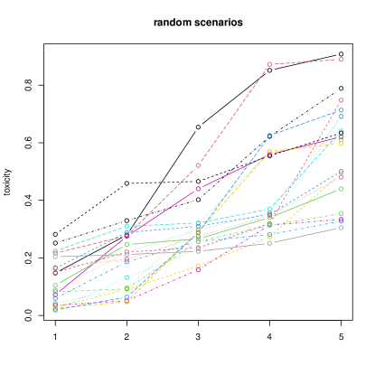
Figure 2: Illustration of the first 20 random scenarios of true toxicity probabilities in the simulation.

4.2 Simulation Results

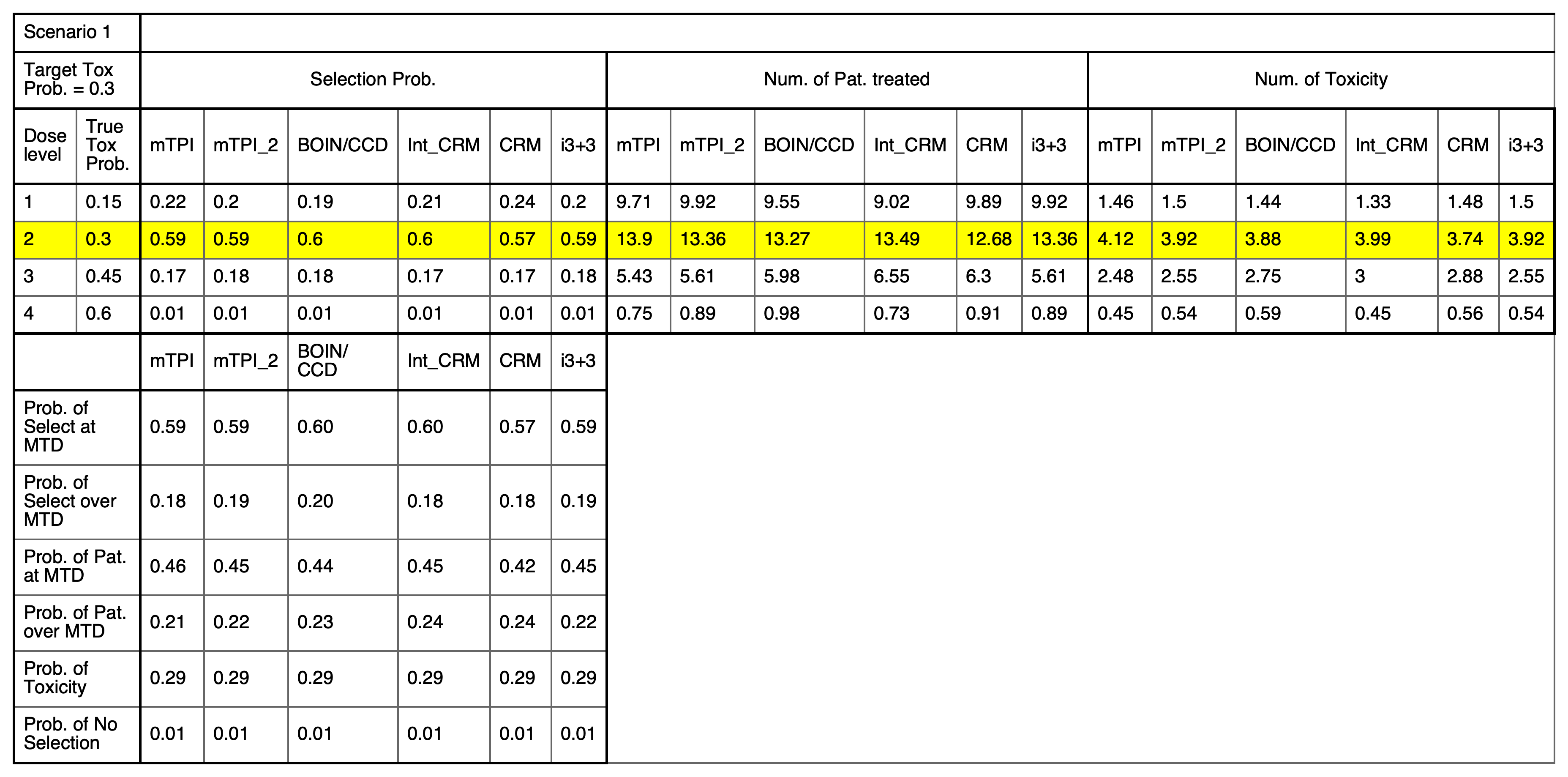
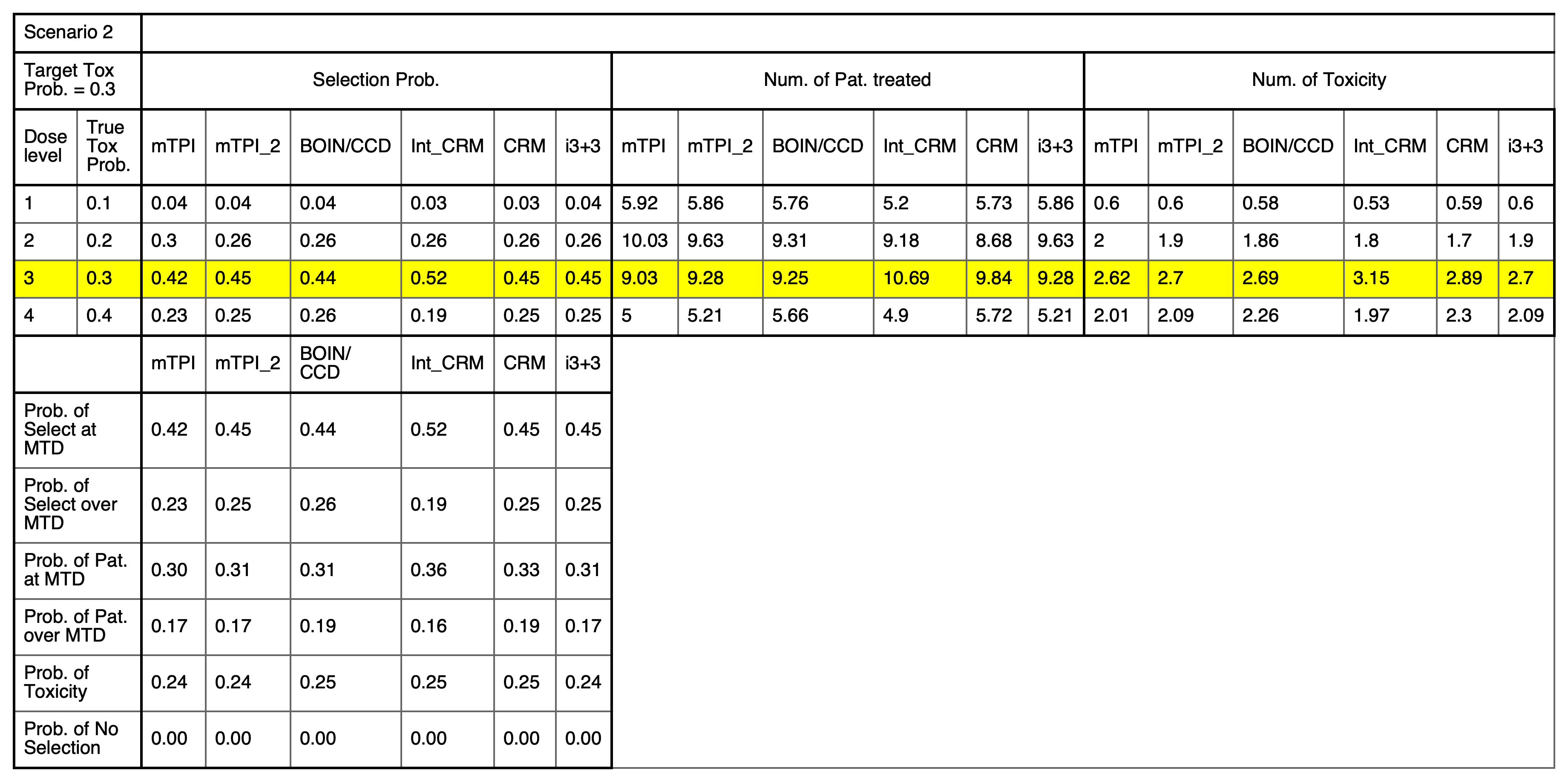
Figure 3: Simulation results of the 5 fixed scenarios with 4 doses levels.

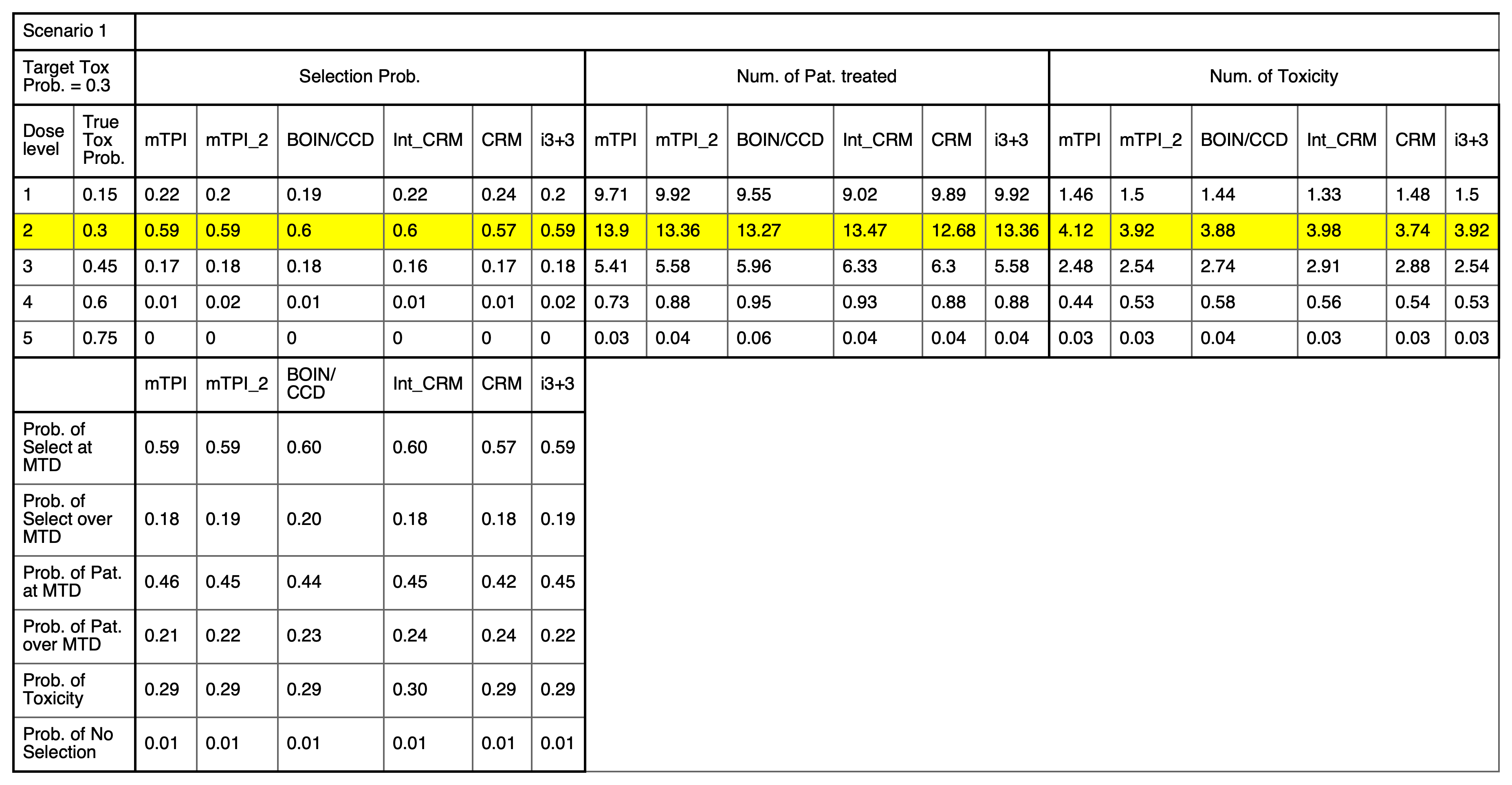
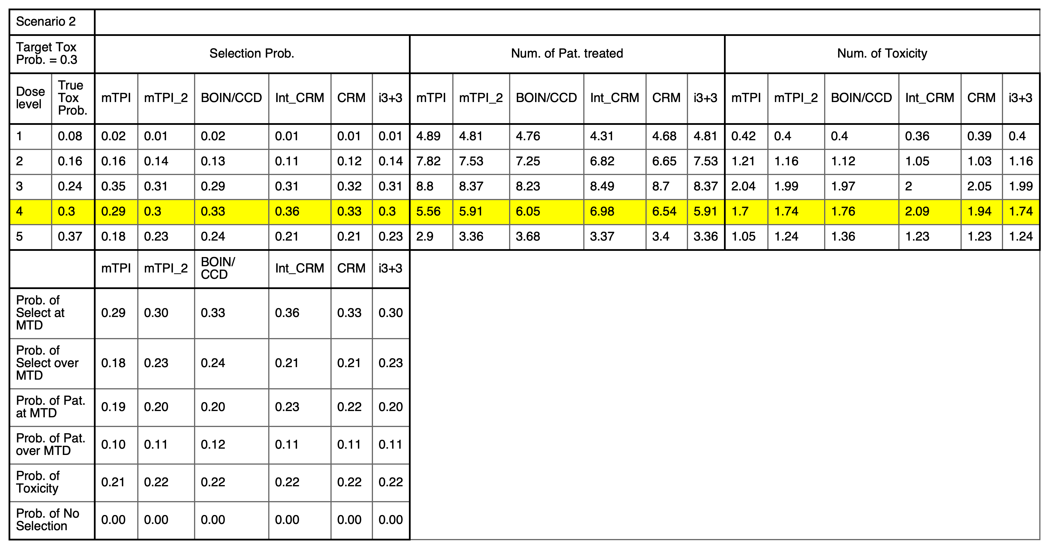
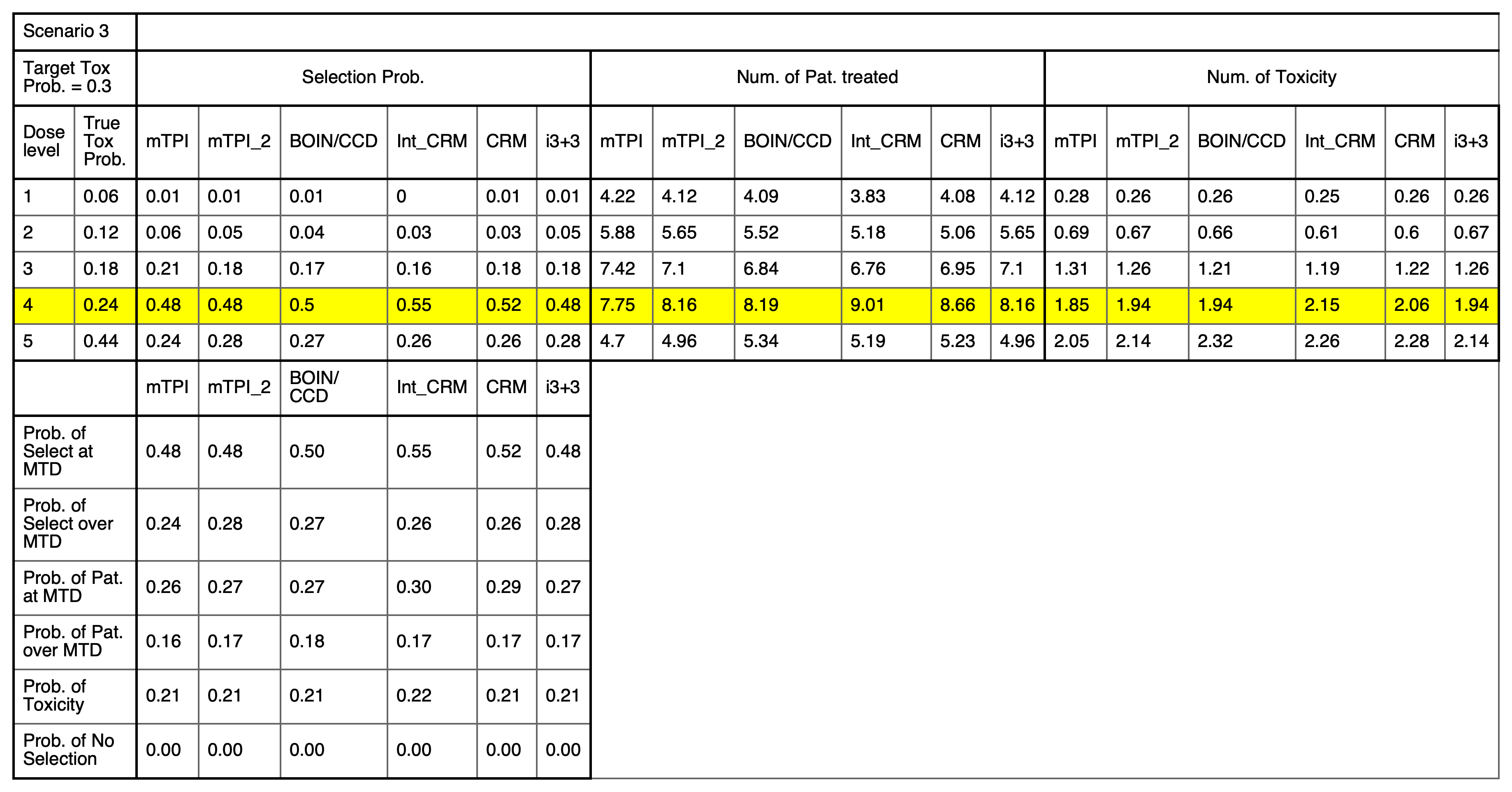
Figure 4: Simulation results of the 5 fixed scenarios with 4 doses levels.

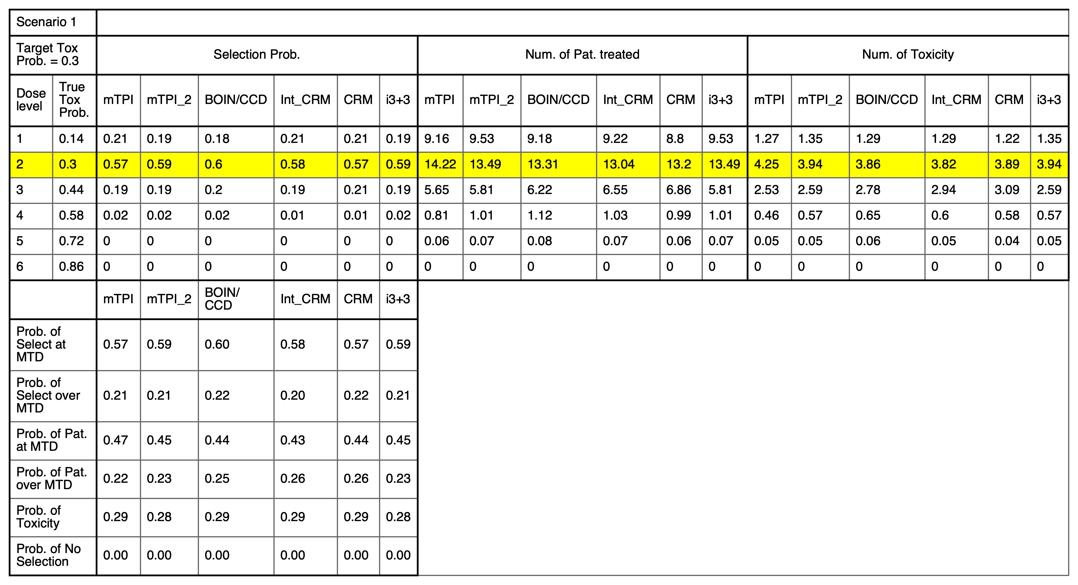
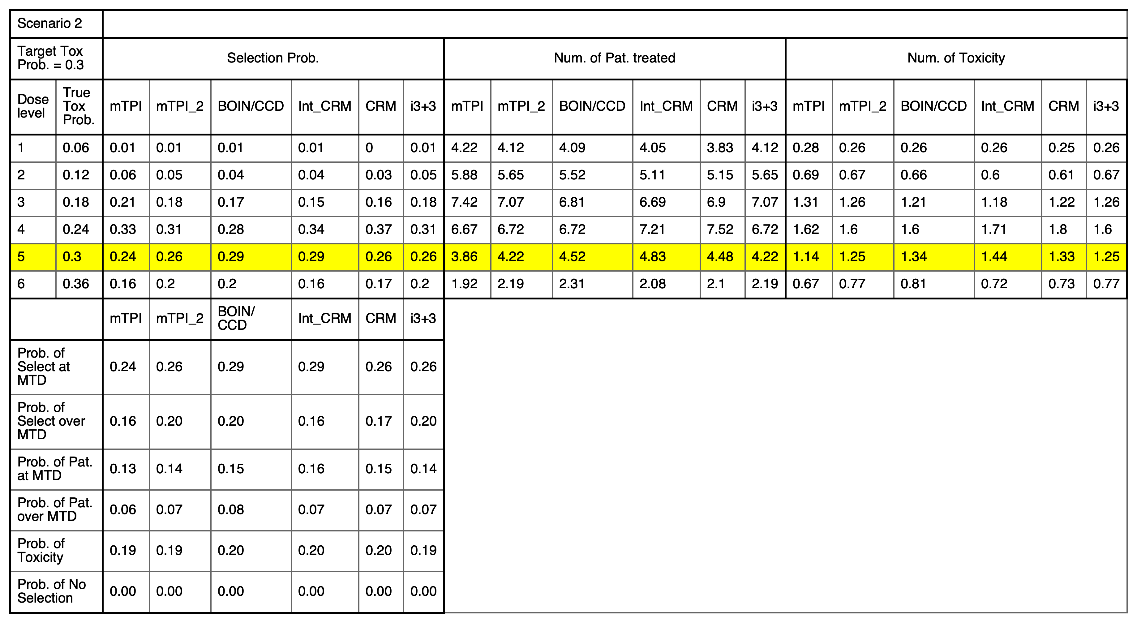
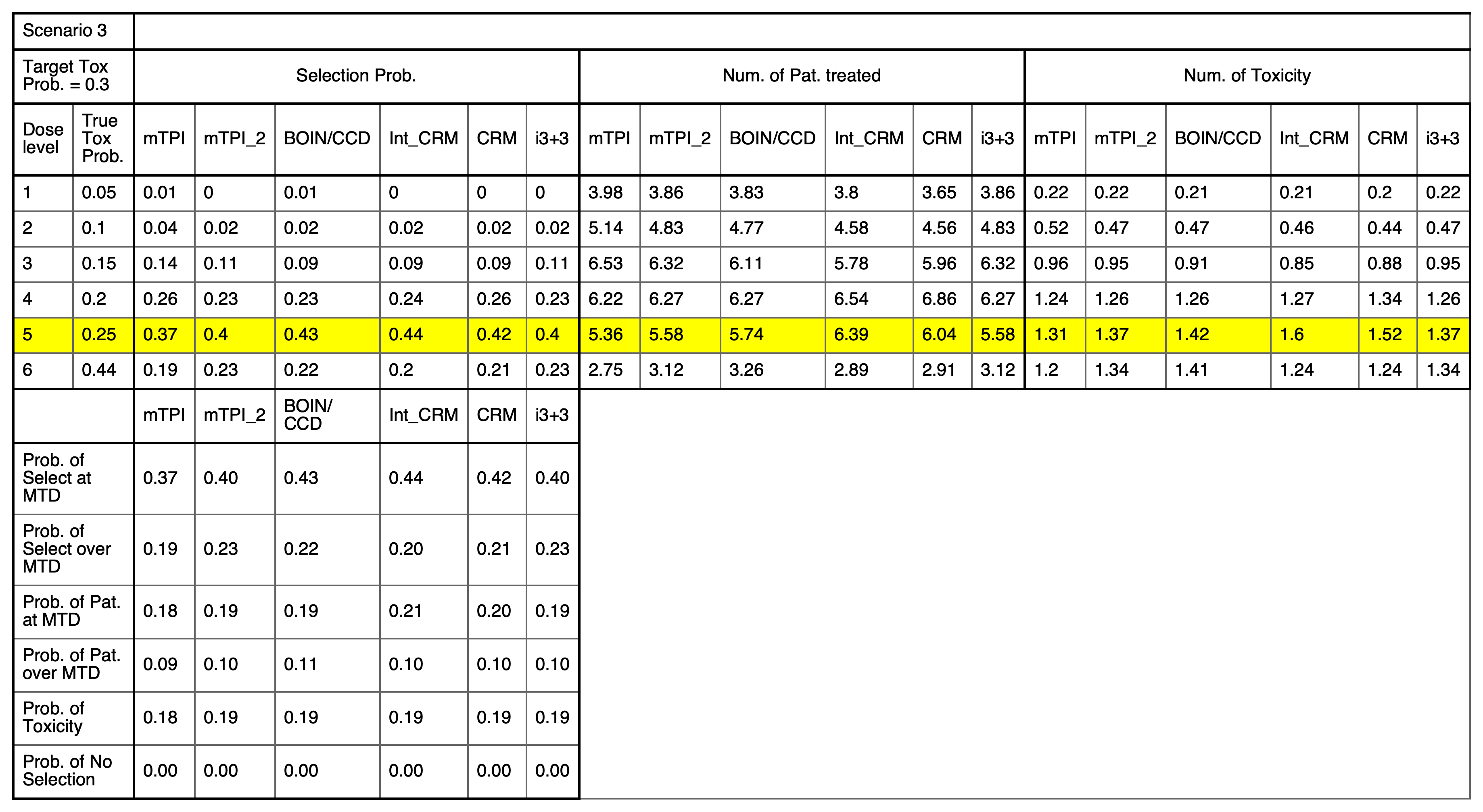
Figure 5: Simulation results of the 5 fixed scenarios with 4 doses levels.

We evaluate the performance of the phase I designs using several metrics, based on their ability to identify the MTD and the safety in dose selection and patient allocation. Table 4 summarizes the means and standard deviations of key performance metrics for the simulation with 1,000 scenarios. All designs show remarkable similarity with the largest mean difference across designs only about 0.02. This highlights the underlying connection of these designs and echoes our findings based on the unified decision framework that can generate most designs as special cases. Figures 3, 4 and 5 in Appendix D present the simulation results of the 15 fixed scenarios.

In general, the five designs tested in the simulation studies exhibit remarkably similar performances. Specifically, they show comparable probabilities (across repeated simulation) of allocating patients to the true MTD, and similar risk of allocating patients to overly toxic doses. The BOIN/CCD and Int-CRM designs yield slightly higher PCS (probability of correct selection of MTD) in some cases, such as scenarios 1 and 4 in Figure 4. However, they also report a higher risk in selecting doses beyond the true MTD. For example, in scenarios 2, 3, and 5 in Figure 4 in Appendix D, the probabilities of over-dosing selection under BOIN, CCD and Int-CRM are higher compared to the other designs.

Table 4: Simulation results of 1,000 random scenarios. Entries are the $\bm{mean}_{sd}$ (across the 1,000 scenarios) proportion of simulated trials for each design and metric.

Metrics	mTPI	mTPI-2	BOIN/CCD	Int-CRM	CRM	i3+3
Correct Sel. of MTD	$0.60_{(0.15)}$	$0.62_{(0.14)}$	$0.62_{(0.14)}$	$0.62_{(0.14)}$	$0.62_{(0.14)}$	$0.62_{(0.14)}$
Sel. over MTD	$0.10_{(0.11)}$	$0.11_{(0.11)}$	$0.12_{(0.12)}$	$0.12_{(0.12)}$	$0.11_{(0.11)}$	$0.11_{(0.11)}$
Pat. at MTD	$0.50_{(0.22)}$	$0.50_{(0.21)}$	$0.50_{(0.20)}$	$0.51_{(0.20)}$	$0.51_{(0.21)}$	$0.50_{(0.21)}$
Pat. over MTD	$0.11_{(0.10)}$	$0.11_{(0.10)}$	$0.12_{(0.11)}$	$0.12_{(0.11)}$	$0.12_{(0.10)}$	$0.11_{(0.10)}$
Tox.	$0.26_{(0.05)}$	$0.26_{(0.05)}$	$0.26_{(0.05)}$	$0.26_{(0.05)}$	$0.26_{(0.05)}$	$0.26_{(0.05)}$
None Sel.	$0.04_{(0.07)}$	$0.04_{(0.07)}$	$0.04_{(0.07)}$	$0.04_{(0.07)}$	$0.04_{(0.07)}$	$0.04_{(0.07)}$

5 Discussion

We have developed a general decision framework for phase I dose-finding designs. We have shown that interval-based designs, like mTPI, mTPI-2, BOIN, CCD, and the model-based design Int-CRM fit into this unified framework.

All designs use the same 0-1 loss function, and all interval designs assume a binomial likelihood function. The prior construction for some designs involves the notion of candidate models. Candidate models are specified assuming different toxic profiles for the doses. Given the model, the mTPI, mTPI-2 and Int-CRM assume continuous prior distributions, using beta or normal distributions truncated to the restricted parameter space implied by the given model. The BOIN and CCD designs use a different approach with a discrete prior on $p_{d}$, supported at three distinct values. Choosing those atoms is challenging and may be difficult to interpret. However, as shown in many simulations conducted and published in literature, the BOIN and CCD designs perform very well in Phase I trials with relatively small sample size.

Additionally, different loss functions can be considered in the proposed framework penalize undesirable actions and outcomes. For examples, the loss for mistakenly making an escalation decision may be larger than for a wrong de-escalation. However, such loses usually lead to more complex and less interpretable decision rules.

It is demonstrated that the designs in this paper perform similarly with comparable reliability and safety. The i3+3 rule-based design is not a part of this framework, but also generates similar operating characteristics, comparable with the other designs. The i3+3 design shares a practically important feature with interval based designs. One can pre-tabulate decision tables, which is a critical feature for the implementation in actual trials. Clinicians can choose a desirable design for phase I clinical trial based on their preference, including the model-based design CRM, the interval designs, mTPI, mTPI-2, BOIN and CCD, and the rule-based design i3+3.

Appendix A

Safety rules: Following the mTPI and mTPI-2 designs [10, 5], two safety rules are added, as ethical constraints to avoid excessive toxicity, to all the designs in the simulation study when needed.

Rule 1: Dose Exclusion.

If the current dose is considered excessively toxic, i.e., $p\{p_{d}>p_{T}\mid Data\}>\xi$, where the threshold $\xi$ is close to 1, say 0.95, then the current and all higher doses are excluded and never used again for the remainder of the trial.

Rule 2: Early Stopping.

If the current dose is the lowest dose (first dose) and is considered excessively toxic according to Rule 1, then stop the trial for safety.

In safety Rules 1 and 2, $Prob\{p_{d}>p_{T}\mid Data\}$ is a function of the cumulative beta distribution $\mbox{Be}(\alpha_{0}+y_{d},\beta_{0}+n_{d}-y_{d})$, and $\alpha_{0}=\beta_{0}=1$ is used by default.

Appendix B

Intervals in Int-CRM design: The intervals in the Int-CRM design are,

$$I_{k}=\{\theta\in[A_{1},A_{T+1}]:|F(k,\theta)-p_{T}|<|F(d,\theta)-p_{T}|,\forall d\neq k\},\;\;\;k=1,\dots,T,$$

which have the form $I_{1}=[\psi_{1}=A_{1},\psi_{2})$, $I_{k}=[\psi_{k},\psi_{k+1}),\;k=2,...,(T-1)$, $I_{T}=[\psi_{T},\psi_{T+1}=A_{T+1}]$. The boundary of the intervals $\psi_{k}$ satisfies the equation

$$F(k-1,\psi_{k})+F(k,\psi_{k})=2p_{T},\;\;\;k=2,...,T.$$

Under the model of Int-CRM,

$$q_{k-1}^{exp(\phi_{k})}+q_{k}^{exp(\phi_{k})}=2p_{T}.$$

Therefore, given the skeleton $(q_{1},...,q_{T})$ and $p_{T}$, we can obtain the numerical solution of the interval boundary by searching over a sequence of $\phi_{k}\in[A_{1},A_{T+1}]$.

Appendix C

Proof of Proposition 1

Proof:

By definition,

$$\mathcal{R}_{d} = \arg\min_{a\in\mathcal{A}}\int\ell(a,p_{d})p(p_{d}\mid\bm{y})dp_{d}=\arg\min_{a\in\mathcal{A}}\int\delta(p_{d}\notin I_{a})p(p_{d}\mid\bm{y})dp_{d}$$

$$= \arg\min_{a\in\mathcal{A}}\int\{1-\delta(p_{d}\in I_{a})\}p(p_{d}\mid\bm{y})dp_{d}=\arg\max_{a\in\mathcal{A}}\int\delta(p_{d}\in I_{a})p(p_{d}\mid\bm{y})dp_{d}$$

$$= \arg\max_{a\in\mathcal{A}}Pr(p_{d}\in I_{a}\mid\bm{y}),$$

which proves the first equation in Proposition 1. In addition, we have

$$\mathcal{R}_{d} = \arg\max_{a\in\mathcal{A}}\int\sum_{k=1}^{3}\delta(p_{d}\in I_{a})p(\bm{y}\mid p_{d})\pi(p_{d}\mid m=k)\pi(m=k)dp_{d}$$ (14)

Since

$$\mathcal{A}=\{E,S,D\},I_{1}=I_{E},I_{2}=I_{S},I_{3}=I_{D},$$

equation 14 becomes

$$\mathcal{R}_{d} = \arg\max_{a\in\mathcal{A}}\int\sum_{k=1}^{3}\delta(p_{d}\in I_{a})p(\bm{y}\mid p_{d})g(p_{d})\delta(p_{d}\in I_{k})\pi(m=k)dp_{d}$$

$$= \arg\max_{k\in\{1,2,3\}}\int p(\bm{y}\mid p_{d})g(p_{d})\delta(p_{d}\in I_{k})\pi(m=k)dp_{d}$$

$$= \arg\max_{k\in\{1,2,3\}}\int p(\bm{y}\mid p_{d})\pi(p_{d}\mid m=k)\pi(m=k)dp_{d}$$

$$= \arg\max_{k\in\{1,2,3\}}\int p(\bm{y}\mid p_{d})\pi(p_{d}\mid m=k)dp_{d}$$

$$= \arg\max_{k\in\{1,2,3\}}Pr(m=k\mid\bm{y})$$

The penultimate equation is true since $\pi(m=k)=\frac{1}{3},\;k=1,2,3.$

$\square$

Proof of Corollary 1

Proof:

Recall the action space $\mathcal{A}=\{E,S,D\}$. Based on Equation (2.2) in Proposition 1, the Bayes’ rule is

$$\mathcal{R}_{d} = \arg\max_{k\in\{1,2,3\}}Pr(m=k\mid y)$$

$$= \arg\max_{k\in\{1,2,3\}}\int p(y\mid p_{d})\pi(p_{d}\mid m=k)dp_{d}$$

$$= \arg\max_{a\in\mathcal{A}}\int p_{d}^{y_{d}}(1-p_{d})^{n_{d}-y_{d}}\cdot C_{k}beta(p_{d};1,1)\delta(p_{d}\in I_{a})dp_{d}$$

$$= \arg\max_{a\in\mathcal{A}}\int p_{d}^{y_{d}}(1-p_{d})^{n_{d}-y_{d}}\frac{beta(p_{d};1,1)\delta(p_{d}\in I_{a})}{\int_{I_{a}}beta(p;1,1)dp}dp_{d}$$

$$= \arg\max_{a\in\mathcal{A}}\int p_{d}^{y_{d}}(1-p_{d})^{n_{d}-y_{d}}\frac{\delta(p_{d}\in I_{a})}{||I_{a}||}dp_{d}=\arg\max_{a\in\mathcal{A}}\mbox{UPM}(I_{a})=R_{mTPI}$$

$\square$

Proof of Corollary 2

Proof:

Based on Equation (2.2), the Bayes’ rule is equal to

$$\mathcal{R}_{d} = \arg\max_{m\in\mathcal{A}_{m}}Pr(m=k\mid y)$$

$$= \arg\max_{m\in\{1,...,K\}}\int p(y\mid p_{d})\pi(p_{d}\mid m=k)dp_{d}$$

$$= \arg\max_{m\in\{1,...,K\}}\int p_{d}^{y_{d}}(1-p_{d})^{n_{d}-y_{d}}\cdot C_{k}beta(p_{d};1,1)\delta(p_{d}\in I_{m})dp_{d}$$

$$= \arg\max_{m\in\{1,...,K\}}\int p_{d}^{y_{d}}(1-p_{d})^{n_{d}-y_{d}}\frac{beta(p_{d};1,1)\delta(p_{d}\in I_{m})}{\int_{I_{m}}beta(p;1,1)dp}dp_{d}$$

$$= \arg\max_{m\in\{1,...,K\}}\int p_{d}^{y_{d}}(1-p_{d})^{n_{d}-y_{d}}\frac{\delta(p_{d}\in I_{m})}{||I_{m}||}dp_{d}$$

$$= \arg\max_{m\in\mathcal{A}_{m}}\mbox{UPM}(I_{m}).$$

$\square$

Proof of Corollary 4

Proof:

Based on Equation (2.2) and the proof of Theorem 1, the Bayes’ rule is

$$\mathcal{R}_{d} = \arg\max_{a\in\{E,S,D\}}{\phi^{\prime}_{a}}^{y_{d}}(1-{\phi^{\prime}_{a}})^{n_{d}-y_{d}},\left\{\begin{array}[]{ll}E,&\hat{p}_{d}\leq\lambda_{1},\\ S,&\lambda_{1}<\hat{p}_{d}<\lambda_{2},\\ D,&\hat{p}_{d}\geq\lambda_{2},\end{array}\right.$$

with $\lambda_{1}=\xi(\phi_{E})=\xi(\xi^{-1}(p_{T}-\epsilon_{1}))=p_{T}-\epsilon_{1}$ and $\lambda_{2}=\xi(\phi_{D})=\xi(\xi^{-1}(p_{T}+\epsilon_{2}))=p_{T}+\epsilon_{2}$. Therefore,

$$\mathcal{R}_{d} = \left\{\begin{array}[]{ll}E&\hat{p}_{d}\leq p_{T}-\epsilon_{1}\\ S&p_{T}-\epsilon_{1}<\hat{p}_{d}<p_{T}+\epsilon_{2}\\ D&\hat{p}_{d}\leq p_{T}+\epsilon_{2}\end{array}\right.\hskip 28.45274pt=\mathcal{R}_{\mbox{CCD}}.$$

$\square$

Proof of Theorem 1

Proof:

According to Proposition 1, under the proposed decision framework, the Bayes’ rule is

$$\mathcal{R}_{d} = \arg\max_{k\in\{1,2,3\}}Pr(m=k\mid y)=\arg\max_{k\in\{1,2,3\}}\int p(y\mid p_{d})\pi(p_{d}\mid m=k)dp_{d}$$ (17)

$$= \arg\max_{k\in\{1,2,3\}}\int p_{d}^{y_{d}}(1-p_{d})^{n_{d}-y_{d}}\delta{(p_{d}=\phi_{k})}dp_{d}$$

$$= \arg\max_{k\in\{1,2,3\}}{\phi_{k}}^{y_{d}}(1-{\phi_{k}})^{n_{d}-y_{d}}=\mbox{arg}\max_{a\in\{E,S,D\}}{\phi_{a}}^{y_{d}}{(1-\phi_{a})}^{n_{d}-y_{d}}.$$

Let $g(p)=p^{y_{d}}(1-p)^{n_{d}-y_{d}},$ then equation 17 becomes

$$\mathcal{R}_{d}=\mbox{arg}\max_{a\in\{E,S,D\}}g(\phi_{a}).$$

When $y_{d}=0$, $g(p)=(1-p)^{n_{d}},$ and $g(p)$ is monotonically decreasing with $p$. When $y_{d}>0$,

$$\frac{dg(p)}{dp}=(y_{d}-n_{d}p)\left\{y_{d}p^{(y_{d}-1)}(1-p)^{n_{d}-y_{d}-1}\right\}.$$

Note that the term $\left\{y_{d}p^{y_{d}-1}(1-p)^{n_{d}-y_{d}-1}\right\}>0$. Then, $\frac{dg(p)}{dp}>0$ if $p\in(0,\frac{y_{d}}{n_{d}})$; and $\frac{dg(p)}{dp}<0$ if $p\in(\frac{y_{d}}{n_{d}},1)$. Therefore, the function $g(p)$ first increases and then decreases with $p$. It only has one mode which is a maximum. In summary, $g(p)$ either monotonically decreases or first increases and decreases with $p$.

$1)$ When $\hat{p}_{d}\leq\lambda_{1}$,

$$\frac{y_{d}}{n_{d}}\leq\lambda_{1}=\frac{log\left(\frac{1-\phi_{E}}{1-\phi_{S}}\right)}{log\left(\frac{\phi_{S}(1-\phi_{E})}{\phi_{E}(1-\phi_{S})}\right)}=\frac{log(1-\phi_{E})-log(1-\phi_{S})}{log(\frac{\phi_{S}}{1-\phi_{S}})-log(\frac{\phi_{E}}{1-\phi_{E}})}.$$

And because $0<\phi_{E}<\phi_{S}<\phi_{D}<1$, we have $log(\frac{\phi_{E}}{1-\phi_{E}})<log(\frac{\phi_{S}}{1-\phi_{S}})<log(\frac{\phi_{D}}{1-\phi_{D}}).$ Therefore, $log(\frac{\phi_{S}}{1-\phi_{S}})-log(\frac{\phi_{E}}{1-\phi_{E}})>0.$ Hence,

$$y_{d}\left\{log(\frac{\phi_{S}}{1-\phi_{S}})-log(\frac{\phi_{E}}{1-\phi_{E}})\right\}\leq n_{d}\left\{log(1-\phi_{E})-log(1-\phi_{S})\right\},$$

and by taking exponentiation on both sides, we have

$$(\frac{\phi_{S}}{1-\phi_{S}})^{y_{d}}(1-\phi_{S})^{n_{d}}\leq(\frac{\phi_{E}}{1-\phi_{E}})^{y_{d}}(1-\phi_{E})^{n_{d}},$$

which leads to

$$\phi_{S}^{y_{d}}(1-\phi_{S})^{n_{d}-y_{d}}\leq\phi_{E}^{y_{d}}(1-\phi_{E})^{n_{d}-y_{d}},$$

i.e., $g(\phi_{S})\leq g(\phi_{E}).$ Since $g(p)$ either monotonically decreases or first increases and then decreases with $p$, and because $\phi_{E}<\phi_{S}<\phi_{D}$ and $g(\phi_{E})\geq g(\phi_{S})$, we have $g(\phi_{E})\geq g(\phi_{S})>g(\phi_{D}).$ Therefore, when $\hat{p}_{d}\leq\lambda_{1}$, $\mathcal{R}_{d}=\mbox{arg}\max_{a\in\{E,S,D\}}g(\phi_{a})=E.$

$2)$ When $\hat{p}_{d}\geq\lambda_{2}$,

$$\frac{y_{d}}{n_{d}}\geq\lambda_{2}=\frac{log\left(\frac{1-\phi_{D}}{1-\phi_{S}}\right)}{log\left(\frac{\phi_{S}(1-\phi_{D})}{\phi_{D}(1-\phi_{S})}\right)}=\frac{log(1-\phi_{D})-log(1-\phi_{S})}{log(\frac{\phi_{S}}{1-\phi_{S}})-log(\frac{\phi_{D}}{1-\phi_{D}})}.$$

Since $log(\frac{\phi_{S}}{1-\phi_{S}})-log(\frac{\phi_{D}}{1-\phi_{D}})<0$,

$$y_{d}\left\{log(\frac{\phi_{S}}{1-\phi_{S}})-log(\frac{\phi_{D}}{1-\phi_{D}})\right\}\leq n_{d}\left\{log(1-\phi_{D})-log(1-\phi_{S})\right\},$$

and

$$(\frac{\phi_{S}}{1-\phi_{S}})^{y_{d}}(1-\phi_{S})^{n_{d}}\leq(\frac{\phi_{D}}{1-\phi_{D}})^{y_{d}}(1-\phi_{D})^{n_{d}},$$

which leads to

$$\phi_{S}^{y_{d}}(1-\phi_{S})^{n_{d}-y_{d}}\leq\phi_{D}^{y_{d}}(1-\phi_{D})^{n_{d}-y_{d}},$$

i.e., $g(\phi_{S})\leq g(\phi_{D}).$ Again, either $g(p)$ monotonically decreases or first increases then decreases with $p$. In either cases, we have $g(\phi_{E})<g(\phi_{S})\leq g(\phi_{D}).$ Therefore, when $\hat{p}_{d}\geq\lambda_{2}$, $\mathcal{R}_{d}=\mbox{arg}\max_{a\in\{E,S,D\}}g(\phi_{a})=D.$

$3)$ When $\lambda_{1}<\hat{p}_{d}<\lambda_{2}$, we have

$$\phi_{S}^{y_{d}}(1-\phi_{S})^{n_{d}-y_{d}}>\phi_{E}^{y_{d}}(1-\phi_{E})^{n_{d}-y_{d}},$$

and

$$\phi_{S}^{y_{d}}(1-\phi_{S})^{n_{d}-y_{d}}>\phi_{D}^{y_{d}}(1-\phi_{D})^{n_{d}-y_{d}},$$

i.e., $g(\phi_{S})>g(\phi_{E})$ and $g(\phi_{S})>g(\phi_{D}).$ Therefore, when $\lambda_{1}<\hat{p}_{d}<\lambda_{2}$, $\mathcal{R}_{d}=\mbox{arg}\max_{a\in\{E,S,D\}}g(\phi_{a})=S.$

$\square$

Appendix D

Operating characteristics for the 15 fixed scenarios in the simulation study. The yellow bar highlights the true MTD. Prob of Select at/over MTD refers to the probability (over repeat simulation) of selecting the true MTD and a dose above the true MTD, respectively. Prob of Pat. at/over MTD refers to the relative frequency of patients assigned at or above the true MTD. Prob of Toxicity refers to the frequency of patients experienced DLT in all simulated trials. Prob of no selection refers to the probability of failing to recommend any dose.

References

• Berger [2013] Berger, J.Β O. (2013). Statistical decision theory and Bayesian analysis. Springer Science & Business Media.
• Cheung [2011] Cheung, Y.Β K. (2011). Dose finding by the continual reassessment method. CRC Press.
• Cheung and Chappell [2002] Cheung, Y.Β K. and Chappell, R. (2002). A simple technique to evaluate model sensitivity in the continual reassessment method. Biometrics 58, 671–674.
• Clertant etΒ al. [2017] Clertant, M., O’Quigley, J., etΒ al. (2017). Semiparametric dose finding methods. Journal of the Royal Statistical Society Series B 79, 1487–1508.
• Guo etΒ al. [2017] Guo, W., Wang, S.-J., Yang, S., Lynn, H., and Ji, Y. (2017). A Bayesian interval dose-finding design addressing Ockham’s razor: mTPI-2. Contemporary clinical trials 58, 23–33.
• Horton etΒ al. [2017] Horton, B.Β J., Wages, N.Β A., and Conaway, M.Β R. (2017). Performance of toxicity probability interval based designs in contrast to the continual reassessment method. Statistics in medicine 36, 291–300.
• Ivanova etΒ al. [2007] Ivanova, A., Flournoy, N., and Chung, Y. (2007). Cumulative cohort design for dose-finding. Journal of Statistical Planning and Inference 137, 2316–2327.
• Jefferys and Berger [1992] Jefferys, W.Β H. and Berger, J.Β O. (1992). Ockham’s razor and Bayesian analysis. American Scientist 80, 64–72.
• Ji etΒ al. [2007] Ji, Y., Li, Y., and NebiyouΒ Bekele, B. (2007). Dose-finding in phase I clinical trials based on toxicity probability intervals. Clinical trials 4, 235–244.
• Ji etΒ al. [2010] Ji, Y., Liu, P., Li, Y., and NebiyouΒ Bekele, B. (2010). A modified toxicity probability interval method for dose-finding trials. Clinical trials 7, 653–663.
• Lee and Cheung [2011] Lee, S.Β M. and Cheung, Y.Β K. (2011). Calibration of prior variance in the Bayesian continual reassessment method. Statistics in medicine 30, 2081–2089.
• Liu etΒ al. [2020] Liu, M., Wang, S.-J., and Ji, Y. (2020). The i3+ 3 design for phase I clinical trials. Journal of Biopharmaceutical Statistics 30, 294–304.
• Liu and Yuan [2015] Liu, S. and Yuan, Y. (2015). Bayesian optimal interval designs for phase I clinical trials. Journal of the Royal Statistical Society: Series C: Applied Statistics pages 507–523.
• Neuenschwander etΒ al. [2008] Neuenschwander, B., Branson, M., and Gsponer, T. (2008). Critical aspects of the Bayesian approach to phase I cancer trials. Statistics in Medicine 27, 2420–2439.
• O’Quigley etΒ al. [1990] O’Quigley, J., Pepe, M., and Fisher, L. (1990). Continual reassessment method: a practical design for phase 1 clinical trials in cancer. Biometrics pages 33–48.
• Storer [1989] Storer, B.Β E. (1989). Design and analysis of phase I clinical trials. Biometrics pages 925–937.
• Thorburn [1918] Thorburn, W.Β M. (1918). The myth of Occam’s razor. Mind 27, 345–353.
• Tighiouart and Rogatko [2010] Tighiouart, M. and Rogatko, A. (2010). Dose finding with escalation with overdose control (EWOC) in cancer clinical trials. Statistical Science 25, 217–226.
• Yan etΒ al. [2017] Yan, F., Mandrekar, S.Β J., and Yuan, Y. (2017). Keyboard: a novel Bayesian toxicity probability interval design for phase I clinical trials. Clinical Cancer Research 23, 3994–4003.
• Yuan etΒ al. [2016] Yuan, Y., Hess, K.Β R., Hilsenbeck, S.Β G., and Gilbert, M.Β R. (2016). Bayesian optimal interval design: a simple and well-performing design for phase I oncology trials. Clinical Cancer Research 22, 4291–4301.