Composing Loop-carried Dependence with Other Loops

Abstract.

Sparse fusion is a compile-time loop transformation and runtime scheduling implemented as a domain-specific code generator. Sparse fusion generates efficient parallel code for the combination of two sparse matrix kernels where at least one of the kernels has loop-carried dependencies. Available implementations optimize individual sparse kernels. When optimized separately, the irregular dependence patterns of sparse kernels create synchronization overheads and load imbalance, and their irregular memory access patterns result in inefficient cache usage, which reduces parallel efficiency. Sparse fusion uses a novel inspection strategy with code transformations to generate parallel fused code for sparse kernel combinations that is optimized for data locality and load balance. Code generated by Sparse fusion outperforms the existing implementations ParSy and MKL on average 1.6$\times$ and 5.1$\times$ respectively and outperforms the LBC and DAGP coarsening strategies applied to a fused data dependence graph on average 5.1$\times$ and 7.2$\times$ respectively for various kernel combinations.

1. Introduction

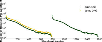
Figure 1. The nonuniform parallelism in the DAGs of sparse incomplete Cholesky and triangular solver (annotated with unfused) and for the joint DAG of the two kernels results in load imbalance. Higher value in the y-axis shows high parallelism in a given wavefront. Wavefront numbers in the x-axis are numbered based on their order of execution.

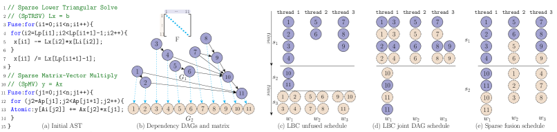
(a)

(b)

(c)

(d)

(e)

Figure 2. Figures 2c-2e show three different schedules for running a sparse lower triangular kernel (SpTRSV) followed by a sparse matrix-vector multiplication (SpMV) as shown in Figure 2b. We choose the number of processors ($r$) to be three. Solid purple ($G_{1}$) and dash-dotted yellow ($G_{2}$) vertices in order represent iterations of SpTRSV and SpMV and edges show the dependencies between iterations. Dashed edges in Figure 2b show dependencies between two kernels and correspond to the nonzero elements of matrix $F$. The unfused implementation schedules each DAG separately as shown in Figure 2c. Two different fused implementations in Figure 2d and 2e use both DAGs and dependencies between kernels to build a fused schedule.

[running example] two different implementations for the input in Listing LABEL:.

Numerical algorithms (Saad, 2003) and optimization methods (Boyd et al., 2004; Stellato et al., 2020; Cheshmi et al., 2020) are typically composed of numerous consecutive sparse matrix computations. For example, in iterative solvers (Saad, 2003) such as Krylov methods (Saad and Malevsky, 1995; Chow and Patel, 2015), sparse kernels that apply a preconditioner or update the residual are repeatedly executed inside and between iterations of the solver. Sparse kernels with loop-carried dependencies, i.e. kernels with partial parallelism, are frequently used in numerical algorithms, and the performance of scientific simulations relies heavily on efficient parallel implementations of these computations. Sparse kernels that exhibit partial parallelism often have multiple wavefronts of parallel computation where a synchronization is required for each wavefront, i.e. wavefront parallelism (Venkat et al., 2016; Govindarajan and Anantpur, 2013). The amount of parallelism varies per wavefront and often tapers off towards the end of the computation, which results in load imbalance. Figure 1 shows with dark lines the nonuniform parallelism for the sparse incomplete Cholesky (SpIC0) and the sparse triangular solve (SpTRSV) kernels when SpTRSV executes after SpIC0 completes. Separately optimizing such kernels exacerbates this problem by adding even more synchronization. Also, opportunities for data reuse between two sparse computations might not be realized when sparse kernels are optimized separately.

Instead of scheduling iterations of sparse kernels separately, they can be scheduled jointly. Wavefront parallelism can be applied to the joint DAG of two sparse computations. A data flow directed acyclic graph (DAG) describes dependencies between iterations of a kernel (Cheshmi et al., 2017; Strout et al., 2018; Hénon et al., 2002). A joint DAG includes all of the dependencies between iterations within and across kernels. The joint DAG of sparse kernels with partial parallelism with the DAG of another sparse kernel provides slightly more parallelism per wavefront without increasing the number of wavefronts. The yellow line in Figure 1 shows how scheduling the joint DAG of SpIC0 and SpTRSV provides more parallelism per wavefront and significantly reduces the number of wavefronts (synchronizations). However, the load balance issues remain, and there are still several synchronizations.

Wavefronts of the joint DAG can be aggregated to reduce the number of synchronizations. DAG partitioners such as Load-Balanced Level Coarsening (LBC) (Cheshmi et al., 2018) and DAGP (Herrmann et al., 2019) apply aggregation, however, when applied to the joint DAG because they aggregate iterations from consecutive wavefronts, load imbalance might still occur. Also, by aggregating iterations from wavefronts in the joint DAG, DAG partitioning methods potentially improve the temporal locality between the two kernels but, this can disturb spatial locality within each kernel. For example, for two sparse kernels that only share a small array and operate on different sparse matrices, optimizing temporal locality between kernels will not be profitable. Finally, even when applied to the DAG of an individual kernel, DAGP and LBC are slow for large DAGs because of the overheads of coarsening (Herrmann et al., 2019). This problem exacerbates when applied to the joint because the joint DAG is typically 2-4$\times$ larger than an individual kernel’s DAG.

We present sparse fusion that creates an efficient schedule and fused code for when a sparse kernel with loop-carried dependencies is combined with another sparse kernel. Sparse fusion uses an inspector to apply a novel Multi-Sparse DAG Partitioning (MSP) runtime scheduling algorithm on the DAGs of the two input sparse kernels. MSP uses a vertex dispersion strategy to balance workloads in the fused schedule, uses two novel iteration packing heuristics to improve the data locality due to spatial and temporal locality of the merged computations, and uses vertex pairing strategies to aggregate iterations without joining the DAGs.

Figure 2 compares the schedule created by sparse fusion (sparse fusion schedule) with the schedules created by applying LBC to the individual DAGs of each sparse kernels (LBC unfused schedule) and LBC applied to the joint DAG (LBC joint DAG schedule). All approaches take the input DAGs in Figure 2b. Solid purple vertices are the DAG of sparse triangular solve (SpTRSV) and the dash-dotted yellow correspond to Sparse Matrix-Vector multiplication (SpMV). LBC is a DAG partitioner that partitions a DAG into a set of aggregated wavefronts called s-partitions that run sequentially, each s-partition is composed of some independent w-partitions. In the LBC unfused schedule in Figure 2c, LBC is used to partition the SpTRSV DAG and will create two s-partitions, i.e. $s_{1}$ and $s_{2}$. The vertices of SpMV are scheduled to run in parallel in a separate wavefront $s_{3}$. This implementation is not load balanced because the number of partitions that can run in parallel differs for each s-partition. In the LBC joint DAG schedule, the DAGs are first joint using the dependency information between the two kernels shown with blue dotted arrows and then LBC is applied to create the two s-partitions in Figure 2d. These s-partitions are also not load balanced, for example $s_{2}$ only has one partition. Sparse fusion uses MSP to first partition the SpTRSV DAG and then disperses the SpMV iterations to create load-balanced s-partitions, e.g. the two s-partitions in Figure 2e have three closely balanced partitions.

SpTRSV solves $Lx=b$ to find $x$ and SpMV performs $y=A*x$ where $L$ is a sparse lower triangular matrix, $A$ is a sparse matrix, and $x$, $b$, and $y$ are vectors. The LBC joint DAG schedule interleaves iterations of two kernels to reuse x. However, this can disturb spatial locality within each kernel because the shared data between the two kernels, $x$, is smaller than the amount of data used within each kernel, $A$ and $L$. With the help of a reuse metric, Sparse fusion realizes the larger data accesses inside each kernel and hence packs iterations to improve spatial locality within each kernel.

We implement sparse fusion as an embedded domain-specific language in C++ that takes the specifications of the sparse kernels as input, inspects the code of the two kernels, and transforms code to generate an efficient and correct parallel fused code. The primary focus of sparse fusion is to fuse two sparse kernels where at least one of the kernels has loop-carried dependence. Sparse fusion is tested on seven of the most commonly used sparse kernel combinations in scientific codes which include kernels such as sparse triangular solver, incomplete Cholesky, incomplete LU, diagonal scaling, and matrix-vector multiplication. The generated code is evaluated against MKL and ParSy with average speedups of 5.1$\times$ and 1.6$\times$ respectively. Sparse fusion compared to fused implementations of LBC, DAGP, and wavefront techniques applied to the joint DAG provides on average 5.1$\times$, 7.2$\times$ and 2.5$\times$ speedup respectively.

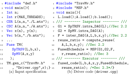
Figure 3. Sparse fusion’s input and the driver code.

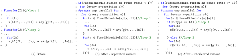
Figure 4. The general form of the sparse fusion code transformation with its two variants, interleaved and separated. I1...In and J1...Jm represent two loop nests. h’ and g’ are data access functions. FusedSchedule contains the schedule for iterations of loops I1, shown with L1 and J1, shown with L2.

[code lowering]the lowering template for fusion.

2. Sparse Fusion

Sparse fusion is implemented as a code generator with an inspector-executor technique that can be used as a library. It takes the input specification shown in Figure 3a and generates the inspector and the executor in Figure 3b. The inspector includes the MSP algorithm and functions that generate its inputs, i.e. dependency DAGs, reuse ratio, and the dependency matrix. The executor is the fused code that is created by the fused transformation.

2.1. Code Generation

Sparse fusion is implemented as an embedded domain-specific language. It takes as input the specification shown in Figure 3a and generates the driver code in Figure 3b. At compile-time, the data types and kernels in Figure 3a are converted to an initial Abstract Syntax Tree (AST) using TM.gen_c() in line 14. Lines 11 and lines 12 in Figure 3a demonstrate how the user specifies the two kernels for the running example in Figure 2 as inputs to Sparse fusion. The corresponding AST for the example is shown in Figure 2a.

At runtime by running the driver code in Figure 3b, the inspector creates a fused schedule, and the executor runs the fused schedule. The inspector first builds inputs to MSP using functions intra_DAG, inter_DAG, and compute_reuse in lines 6–10 in Figure 3b and then calls MSP in line 11 to generate FusedSchedule for r threads. Then the executor code, fused_code in line 14 in Figure 3b, runs in parallel using the fused schedule.

2.2. The Inspector in Sparse Fusion

The MSP algorithm requires kernel-specific inputs. Its inputs are the dependency matrix between kernels, the DAG of each kernel, a reuse ratio. Sparse fusion analyzes the kernel code, available from its AST, to generate inspector components that create these inputs.

Dependency DAGs: Lines 6–7 in Figure 3b use an internal domain-specific library to generate the dependency DAG of each kernel. General approaches such as work by Mohammadi et al. (Mohammadi et al., 2019) can also be used to generate the DAGs, however, that will lead to higher inspection times compared to a domain-specific approach. For example, with domain knowledge, sparse fusion will use the $L$ matrix as the SpTRSV DAG $G_{1}$ in Figure 2b. Each nonzero $L_{ij}$ represents a dependency from iteration $i$ to $j$.

Dependency Matrix $F$: MSP uses the dependency information between kernels to create a correct fused schedule. By running the inter_DAG function, sparse fusion creates this information and stores it in matrix $F$. To generate inter_DAG, sparse fusion finds dependencies between statements of the two kernels by analyzing the AST. Each nonzero $F_{i,j}$ represents a dependency from iteration $j$ of the first loop, i.e. column $j$ of $F$, to iteration $i$ of the second loop, i.e. row $i$ of $F$. In Figure 2a, there exists a read after write (flow) dependency between statements x[i1] in line 5 and x[j1] in line 13. As a result, sparse fusion generates the function shown in Listing 1. The resulting $F$ matrix, generated at runtime, is shown in Figure 2b.

⬇

for(i1=0; i1<n; i1++){

j1 = i1;

if(A.p[j1] < A.p[j1+1] )

F[j1].append(i1); }

Listing 1: inter_DAG function for the example in Figure 2a.

Reuse Ratio: MSP uses a reuse ratio based on the memory access patterns of the kernels to decide whether to improve locality within each kernel or between the kernels. The inspector in line 9 in Figure 3b computes the reuse ratio metric. The metric represents the ratio of common to total memory accesses of the two kernels, i.e. $\frac{\text{common memory access}}{max(\text{kernel1 accesses, kernel2 accesses)}}$. For a reuse ratio larger than one, the number of common memory accesses between the two kernels is larger than the accesses inside a kernel. Sparse fusion estimates memory accesses using the ratio of the size of common variables over the maximum of the total size of variables amongst the kernels. For the running example, the code generated for compute_reuse is 2*x.n / max(A.size+x.n+y.n,L.size+
x.n+b.n). Since x is smaller than $L$ or $A$, the reuse ratio is less than one.

2.3. Fused Code

To generate the fused code, a fused transformation is applied to the initial AST at compile-time and two variants of the fused code are generated, shown in Figure 4. The transformation variants are separated and interleaved. The fused code uses the reuse ratio at runtime to select the correct variant for the specific input. The variable fusion in line 1 of Figure 4b and 4c is set to False if MSP determines fusion is not profitable. Figure 4a shows the sequential loops in the AST, which are annotated with Fuse, and are transformed to the separated and interleaved code variants as shown in order in Figures 4b and 4c. The separated variant is selected when the reuse ratio is smaller than one. In this variant, iterations of one of the loops run consecutively without checking the loop type. The interleaved variant is chosen when the reuse ratio is larger than one. In this variant, iterations of both loops should run interleaved, and the variant checks the loop type per iteration as shown in lines 6 and 10 in Figure 4c.

3. Multi-Sparse DAG Partitioning

(a)

(b)

(c)

(d)

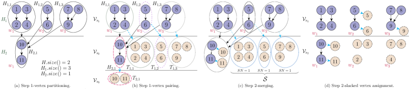
(e)

Figure 5. Stages of MSP for DAGs $G_{1}$ and $G_{2}$ and matrix $F$ in the running example shown in Figure 2b where the reuse ratio ($reuse\_ratio$) is smaller than one and number of processors ($r$) is three. The first step of the algorithm selects $G_{1}$ and creates $H$ partitioning for three processors using the LBC algorithm as shown in Figure 5a. Then it pairs each $H_{i,j}$ through dependencies in matrix $F$ to create partitioning $T$ of $G_{2}$ as shown in Figure 5b. The partitions with the same line pattern/color are pair partitions. In the second step, MSP merges pair partitions that cannot be dispersed such as first w-partitions of s-partitions 2 and 3 ($\mathcal{V}_{s_{3},w_{1}}$ and $\mathcal{V}_{s_{2},w_{1}}$) in Figure 5b, these are merged into $\mathcal{V}_{s_{2},w_{1}}$ in Figure 5c. Slack vertices, which are denoted as $\mathcal{S}$ are shown with blue dotted circles in Figure 5c. Slack vertices are assigned into imbalanced w-partitions as shown in Figure 5d. Since the reuse ratio is smaller than one, vertices inside each partition are packed separately as shown in Figure 2e.

[running example] two different implementations for the input in Listing LABEL:.

Sparse fusion uses the multi-sparse DAG partitioning (MSP) algorithm to create an efficient fused partitioning that will be used to schedule iterations of the fused code. MSP partitions vertices of the DAGs of the two input kernels to create parallel load-balanced workloads for all cores while improving locality within each thread. This section describes the inputs, output, and three steps of the MSP algorithm using the running example in Figures 2 and  5.

Input :  $G_{1}(V_{1},E_{1},c_{1})$, $G_{2}(V_{2},E_{2},c_{2})$, $F$, $r$, $reuse\_ratio$

Output :  $\mathcal{V}$

/* (i) Vertex partitioning and partition pairing */

1 if $|E_{2}|>0$ then

2      

3      $[H,k]$ = LBC($G_{2}$, $r$).list(), $T=\emptyset$, $\mathcal{V}=\emptyset$

       /* Backward pairing */

4       for $(i=1:H.size())$  do

5             for $(j=1:H_{i}.size())$  do

6                   $T_{i,j}=$ BFS($H_{i,j},F,G_{1}$)

7                   $\mathcal{V}.add(T_{i,j},H_{i,j})$

8                  

9             end for

10            

11       end for

12       if $|\mathcal{V}|>2\times(|V_{1}|+|V_{2}|)$  then   $\mathcal{V}$.fusion = False, exit()

13      

14else

15       $[H,k]$ = LBC($G_{1}$, $r$).list(), $T=\emptyset$, $\mathcal{V}=\emptyset$

       /* Forward pairing */

16       for $(i=1:H.size())$  do

17             for $(j=1:H_{i}.size())$  do

18                   $T_{i,j}=$ BFS($H_{i,j},F^{T},G_{2}$)

19                  

20                  $U_{i,j}=T_{i,j}$.remove_uncontained($F$)

21                   $\mathcal{V}.add(H_{i,j},T_{i,j},U_{i,j})$

22                  

23             end for

24            

25       end for

26      

27 end if

28

/* (ii) Merging and slacked vertex assignment */

29 $\mathcal{S}$ = slack_info($\mathcal{V}$)

30 for (every w-partition pair $(w,w^{\prime})\in\mathcal{V}.pairs)$ do

31       if $(SN(w)=0)\land(SN(w^{\prime})=0)$ then  $\mathcal{V}$.merge($w$,$w^{\prime}$)

32      

33 end for

34

35$\mathcal{V}=\mathcal{V}-\mathcal{S}$, $\epsilon=|\mathcal{V}|\times 0.001$

36 for $(i=1:\mathcal{V}.b)$  do

37       for $(j=1:m_{i})$  do

38             if max_diff($\mathcal{V}_{s_{i}},\mathcal{V}_{s_{i},w_{j}}$) ¿ $\epsilon\land\mathcal{S}\neq\emptyset$  then  $\mathcal{S}=\mathcal{V}_{s_{i},w_{j}}$.balance_with_pair($\mathcal{S}$)

39             if max_diff($\mathcal{V}_{s_{i}},\mathcal{V}_{s_{i},w_{j}}$) ¿ $\epsilon\land\mathcal{S}\neq\emptyset$  then  $\mathcal{S}=\mathcal{V}_{s_{i},w_{j}}$.balance_with_slacks($\mathcal{S}$)

40            

41       end for

42      if $\mathcal{S}\neq\emptyset$ then  $\mathcal{S}=\mathcal{V}_{s_{i}}$.assign_even($\mathcal{S}$)

43      

44 end for

/* (iii) Packing */

45 if $reuse\_ratio\geq 1$ then  $\mathcal{V}$.interleaved_pack($F$) 

46else  $\mathcal{V}$.separated_pack() 

47

48

Algorithm 1 The MSP algorithm.

3.1. Inputs and Output to MSP

The inputs to MSP (shown in Algorithm 1) are two DAGs $G_{1}$ and $G_{2}$ from in order lexicographically first and second input kernels, and the inter-DAG dependency matrix $F$ that stores the dependencies between kernels. A DAG shown with $G_{j}(V_{j},E_{j},c)$ has a vertex set $V_{j}$ and an edge set $E_{j}$ and a non-negative integer weight $c(v_{i})$ for each vertex $v_{i}\in V_{j}$. The vertex $v_{i}$ of $G_{j}$ represents iteration $i$ of a kernel and each edge shows a dependency between two iterations of a kernel. $c(v_{i})$ is the computational load of a vertex and is defined as the total number of nonzeros touched to complete its computation. Because sparse matrix computations are generally memory bandwidth-bound, $c(v_{i})$ is a good metric to evaluate load balance in the algorithm (Cheshmi et al., 2018). $F$ is stored in the compressed sparse row (CSR) format and $F_{i}$ is used to extract the set of vertices in $G_{1}$ that $v_{i}\in V_{2}$ depends on. Other inputs to the algorithm are the number of requested partitions $r$, which is set to the number of cores, and the reuse ratio discussed in section 2.2.

The output of MSP is a fused partitioning $\mathcal{V}$ that has $b\geq 1$ s-partitions, each s-partition contains up to $k>1$ w-partitions, where $k\leq r$. MSP creates $b$ disjoint s-partitions from vertices of both DAGs, shown with $\mathcal{V}_{s_{i}}$ where $\cup_{i=0}^{b}\mathcal{V}_{s_{i}}=V_{1}\cup V_{2}$. Each s-partition includes vertices from a lower bound and upper bound of wavefront numbers shown with $s_{i}=[lb_{i}..ub_{i})$ as well as some slack vertices. For each s-partition $\mathcal{V}_{s_{i}}$, MSP creates $m_{i}\leq k$ independent w-partitions $\mathcal{V}_{s_{i},w_{j}}$ where $\mathcal{V}_{s_{i},w_{1}}\cup...\cup\mathcal{V}_{s_{i},w_{m_{i}}}=\mathcal{V}_{s_{i}}$. Since w-partitions are independent, they can run in parallel.

Example. In Figure 2b, the SpTRSV DAG $G_{1}$, the SpMV DAG $G_{2}$, the inter-DAG dependency matrix $F$ are inputs to MSP. Other inputs to MSP are $r$=3 and the $reuse\_ratio$. The fused partitioning shown in Figure 2e has two s-partitions ($b$=2). The first s-partition has three w-partitions ($m_{1}$=3) shown with $\mathcal{V}_{s_{1}}=\{[\underline{1},\underline{2},\underline{3},\underline{4}];[\underline{5},\underline{6},5,6];[\underline{7},\underline{8},\underline{9},9]\}$, the underscored vertices belong to $G_{1}$.

3.2. The MSP Algorithm

Algorithm 1 shows the MSP algorithm. It takes the inputs and goes through three steps of (1) vertex partitioning and partition pairing with the objective to aggregate iterations without joining the DAGs of the inputs kernels; (2) merging and slack vertex assignment to reduce synchronization and to balance workloads; and (3) packing to improve locality.

3.2.1. Vertex Partitioning and Partition Pairing.

The first step of MSP partitions one of the input DAGs $G_{1}$ or $G_{2}$, and then uses that partitioning to partition the other DAG. The created partitions are stored in $\mathcal{V}$. Partitioning the joint DAG is complex and might not be efficient because of the significantly larger number of edges and vertices added compared to the individual DAG of each kernel. Instead, MSP ignores the dependencies across kernels and first creates a partitioning from one of the DAGs with the help of vertex partitioning. Then the other DAG is partitioned using a partition pairing strategy. The DAG that is partitioned first is the head DAG and the other is the tail DAG. A head DAG choice strategy is used to select the head DAG.

Vertex partitioning. MSP uses the LBC DAG partitioner (Cheshmi et al., 2018) to construct a partitioning of the head DAG in lines 1 and 1 of Algorithm 1 by calling the function LBC. The resulting partitioning has a set of disjoint s-partitions. Each s-partition contains $k$ disjoint w-partitions which are balanced using vertex weights. Disjoint w-partitions ensure all w-partitions within s-partitions are independent. The created partitions are stored in a two-dimensional list $H$ using list, e.g. w-partition $w_{j}$ of s-partition $s_{i}$ is stored in $H_{ij}$.

Partition pairing. The algorithm then partitions the tail DAG with forward pairing, if $G_{1}$ is the head DAG, or with backward pairing, if $G_{2}$ is the head DAG. With the pairing strategy, some of the partitions of the tail DAG are paired with the head DAG partitions. Pair-partitions are self-contained so that they execute in parallel if assigned to the same s-partition. The created partitions are put in the fused partitioning $\mathcal{V}$ to be used in step two. The following first describes the condition for partitions to be self-contained and then explains the forward and backward pairing strategies.

Pair partitions $H_{ij}$ and $T_{ij}$ are called self-contained if all reachable vertices from a breadth first search (BFS) on $\forall v\in H_{ij}\cup T_{ij}$ through vertices of $G_{1}$ and $G_{2}$ are in $H_{ij}\cup T_{ij}$. Self-contained pair partition $(H_{ip},T_{ip})$ and pair partition $(H_{iq},T_{iq})$ can execute in parallel without synchronization if in the same wavefront $i$, i.e. $\forall 1\leq i\leq b\land(1\leq p,q\leq m_{i})$. Partitions that do not satisfy this condition create synchronizations in the final schedule.

The backward pairing strategy visits every partition $H_{i,j}$ and performs a BFS (line 1) from vertex $v_{l}\in H_{i,j}$ to its dependent vertices in $G_{1}$ which are reachable through $F_{l}$. Reachable vertices are stored in $T_{ij}$. The partitions in $H$ and $T$ are assigned a w- and s-partition and are then put in the fused partitioning $\mathcal{V}$ (via add in line 1). The assigned s- and w-partitions for $H_{ij}$ are $s_{i+1}$ and $w_{j}$ respectively, i.e. $\mathcal{V}_{s_{i+1},w_{j}}$. $T_{ij}$ should be executed before $H_{ij}$ thus is placed in s-partition $s_{i}$ or $\mathcal{V}_{s_{i},w_{m_{i}+1}}$, where $m_{i}$ is number of w-partitions in $\mathcal{V}_{s_{i}}$ at this point. If a vertex in $H_{i,j}$ depends on more than one vertex in $G_{1}$, some vertices are replicated in different $T$ partitions. While replication leads to redundant computation, it ensures that the pair partition $(H_{i,j},T_{i,j})$ is self-contained because vertices that depend on the vertices in $H_{i,j}$ will be included in $T_{i,j}$. MSP performs fusion only if profitable, hence fusion is disabled (by setting fusion to False) if the number of redundant computations go beyond a threshold. This threshold is $2\times(|V_{1}|+|V_{2}|)$ in line 1 and is defined as the sum of vertices of both DAGs.

The forward pairing strategy iterates over every partition $H_{i,j}$ and performs a BFS from vertex $v_{l}\in H_{i,j}$ to its reachable vertices in $G_{2}$ through $F^{T}_{l}$, see lines 1–1 in Algorithm 1. The list of reachable vertices are stored in $T_{i,j}$ via BFS in line 1. If a vertex $v_{m}$ in $T_{i,j}$ depends on vertex $v_{l}$ in $G_{1}$ and $v_{l}$ does not exist in $H_{i,j}$ then $v_{m}$ should be removed to ensure $(H_{i,j},T_{i,j})$ is self contained. The remove_uncontained function in line 1 removes vertex $v_{m}$ and puts it in partition $U_{i,j}$. Finally, the created partitions are assigned to the fused partitioning $\mathcal{V}$ via add in line 1 as follows: $\mathcal{V}_{s_{i},w_{j}}=H_{i,j}$, $\mathcal{V}_{s_{i+1},w_{m_{i+1}+1}}=T_{i,j}$, $\mathcal{V}_{s_{i+1},w_{m_{i+1}+1}}=U_{i,j}$.

The head DAG choice. MSP chooses the DAG with edges as the head DAG to improve locality. Locality is improved because the head DAG is partitioned with LBC. LBC creates well-balanced partitions with good locality when applied to DAGs with edges. Selecting $G_{2}$ as the head DAG reduces inspector overhead. If both $G_{1}$ and $G_{2}$ are DAGs of kernels with dependency, then $G_{2}$ is chosen as the head DAG to reduce inspector overhead. When $G_{2}$ is partitioned first, MSP chooses backward pairing which is more efficient compared to forward pairing. Forward pairing traverses $F$ and its transpose $F^{T}$ and thus performs $2*nnz_{F}+2*n$ operations where $nnz_{F}$ is the number of nonzeros in $F$. However, backward pairing only traverses $F$ and performs $nnz_{F}+n$ operations.

Example. Figures 5b shows the output of MSP after the first step for the inputs in Figure 2b. MSP chooses $G_{1}$ as the head DAG because it has edges ($|E_{1}|>1$), $G_{2}$ has no edges. In vertex partitioning, $G_{1}$ is partitioned with LBC to create up to three w-partitions (because $r=3$) per s-partition. The created partitions are shown in Figure 5a and are stored in $H$. The first s-partition $\mathcal{V}_{s_{1}}$ is stored in $H_{1}$ and its three w-partitions are indexed with $H_{1,1}$, $H_{1,2}$, and $H_{1,3}$. Similarly, $\mathcal{V}_{s_{2}}$ is stored $H_{2}$ and its only w-partition is in $H_{2,1}$. Figure 5b shows the output of partition pairing. Since $G_{1}$ is the head DAG, MSP uses forward pairing and performs a BFS from each partition in $H$ to create self-contained pair partitions stored in $T$. For example, a BFS from $H_{1,1}=\{\underline{1},\underline{2},\underline{3},\underline{4}\}$ creates $T_{1,1}=\{1,2,3,4\}$. Since $T_{1,1}$ and $H_{1,1}$ are self-contained, no vertices are removed from $T_{1,1}$ and thus $U_{1,1}=\emptyset$. Finally, MSP puts $H_{1,1}$ and $T_{1,1}$ in $\mathcal{V}_{s_{1},w_{1}}$ and $\mathcal{V}_{s_{2},w_{2}}$ respectively, and adds $(\mathcal{V}_{s_{1},w_{1}},\mathcal{V}_{s_{2},w_{2}})$ to $\mathcal{V}.pairs$. The final partitions and pairings as shown in Figure 5b are: $\mathcal{V}=[\{H_{1,1},H_{1,2},H_{1,3}\},\{H_{2,1},T_{1,1},T_{1,2},T_{1,3}\},\{T_{2,1}\}]=[\{\{\underline{1},\underline{2},\underline{3},\underline{4}\},\\ \{\underline{5},\underline{6}\},\{\underline{7},\underline{8},\underline{9}\}\},\{\{\underline{10},\underline{11}\},\{1,2,3,4\},\{5,6\},\{7,8,9\}\},\{\{10,11\}\\ \}]$ and the pairing information is: $\mathcal{V}.pairs=\{(\mathcal{V}_{s_{1},w_{1}},\mathcal{V}_{s_{2},w_{2}}),\\ (\mathcal{V}_{s_{1},w_{2}},\mathcal{V}_{s_{2},w_{3}}),(\mathcal{V}_{s_{1},w_{3}},\mathcal{V}_{s_{2},w_{4}}),(\mathcal{V}_{s_{2},w_{1}},\mathcal{V}_{s_{3},w_{1}})\}$.

3.2.2. Merging and Slack Vertex Assignment.

The second step of MSP reduces the number of synchronizations by merging some of the pair partitions in a merging phase. It also improves load balance by dispersing vertices across partitions using slacked vertex assignment.

Slack definitions: A vertex $v$ can always run in its wavefront number $l(v)$. However, the execution of vertex $v$ can sometimes be postponed up to $SN(v)$ wavefronts without having to move its dependent vertices to later wavefronts. $SN(v)$ is the slack number of $v$ and is defined as $SN(v)=P_{G}-l(v)-height(v)$ where $height(v)$ is the maximum path from a vertex $v$ to a sink vertex (a sink vertex is a vertex without any outgoing edge), $P_{G}$ is the critical path of $G$, and $l(v)$ is the wavefront number of $v$. A vertex with a positive slack number is a slack vertex. To compute vertex slack numbers efficiently, instead of visiting all vertices, MSP iterates over partitions and computes the slack number of each partition in the partitioned DAG, i.e. partition slack number. The computed slack number for a partition is assigned to all vertices of the partition. As shown in line 1 of Algorithm 1, all partition slack numbers of $\mathcal{V}$ are computed via slack_info and are stored in $\mathcal{S}$. For example, because vertices in $\mathcal{V}_{s_{2},w_{3}}$ can be postponed one wavefront, from s-partition 2 to 3, their slack number is 1. Vertices in w-partitions $\mathcal{V}_{s_{2},w_{1}}$ and $\mathcal{V}_{s_{3},w_{1}}$ can not be moved because their slack numbers are zero.

Merging. MSP finds pair partitions with partition slack number of zero and then merges them as shown in lines 1-1. Since pair partitions are self contained, merging them does not affect the correctness of the schedule. Algorithm 1 visits all pair partitions $(w,w^{\prime})$ in $\mathcal{V}.pairs$ and merges them using the merge function in line 1 if their slack numbers are zero, i.e. $SN(w)=0$ and $SN(w^{\prime})=0$. The resulting merged partition is stored in $\mathcal{V}$ in place of the w-partition with the smaller s-partition number.

Slacked vertex assignment. The algorithm then uses slacked vertex assignment to approximately load balance the w-partitions of an s-partition using a cost model. The cost of w-partition $w\in\mathcal{V}_{s_{i}}$ is defined as $cost(w)=\sum_{v\in w}c(v)$. A w-partition is balanced if the maximal difference of its cost and the cost of other w-partitions in its s-partition is smaller than a threshold $\epsilon$. The maximal difference for a w-partition inside a s-partition is computed by subtracting its cost from the cost of the w-partition (from the same s-partition) with the maximum cost.

MSP first removes all slacked vertices $\mathcal{S}$ from the fused partitioning $\mathcal{V}$ in line 1. It then goes over every s-partition $i$ and w-partition $j$ and balances $\mathcal{V}_{s_{i},w_{j}}$ by assigning a slacked vertex to it where possible. W-partition $\mathcal{V}_{s_{i},w_{j}}$ becomes balanced with vertices from its pair partition using the function balance_with_pair in line 1. If $\mathcal{V}_{s_{i},w_{j}}$ is still imbalanced, balance_with_slacks in line 1 balances the w-partition using the slacked vertices $v_{l}\in\mathcal{S}$ that satisfy the following condition $l(v_{l})<i<(l(v_{l})+SN(v_{l}))$. Slack vertices in $\mathcal{S}$ that depend on each other are dispersed as a group to the same w-partition for correctness. In line 1, slacked vertices in $\mathcal{S}$ that are not postponed to later s-partitions are evenly divided between the w-partitions of the current s-partition ($\mathcal{V}_{s_{i}}$) using the assign_even function.

Example. Figure 5d shows the output of the second step of MSP from the partitioning in Figure 5b. First pair partitions $(\mathcal{V}_{s_{2},w_{1}},\mathcal{V}_{s_{3},w_{1}})$, shown with red dash-dotted circles in Figure 5b, are merged because their slack numbers are zero. The resulting merged partition is placed in $\mathcal{V}_{s_{2},w_{1}}$ to reduce synchronization as shown in Figure 5c. Then slacked vertex assignment balances the w-partitions in Figure 5c. The balanced partitions are shown in Figure 5d. The slacked vertices $S$, are shown with dotted blue circles in Figure 5c. The w-partitions in $\mathcal{V}_{s_{1}}$ are balanced using vertices of their pair partitions, e.g. the yellow dash-dotted vertices 5 and 6 are moved to $w_{2}$ in $\mathcal{V}_{s_{1}}$ as shown in Figure 5d. balance_with_slacks is used to balance partitions in $\mathcal{V}_{s_{2}}$. This is because the vertices in $S$ do not belong to the pair partitions of the w-partitions in $\mathcal{V}_{s_{2}}$. However, since the slack vertices in $S$ can execute in either s-partition two or three because they are from s-partition one and have a slack number of one, they are used to balance the w-partitions in $\mathcal{V}_{s_{2}}$.

3.2.3. Packing.

The third step of MSP reorders the vertices inside a w-partition to improve data locality for a thread within each kernel or between the two kernels. The previous steps of the algorithm create w-partitions that are composed of vertices of one or both kernels however the order of execution is not defined. Using the reuse ratio, the order at which the nodes in a w-partition should be executed is determined with a packing strategy. MSP has two packing strategies: (i) in interleaved packing, the vertices of the two DAGs in a w-partition are interleaved for execution and (ii) in separated packing the vertices of each kernel are executed separately. Interleaved packing improves temporal locality between kernels while separated packing enhances spatial and temporal locality within kernels. When the reuse ratio is greater than one, in line 1 of Algorithm 1 function interleaved_pack is called to interleave iterations of the two kernels based on F. Otherwise, separated_pack is called (line 1) to pack iterations of each kernel separately.

Example. Figure 2e shows the output of MSP’s third step from the partitioning in Figure 5d. Since the reuse ratio is smaller than one separated packing is chosen thus $\mathcal{V}_{s_{2},w_{1}}$ is stored as $\mathcal{V}_{s_{2},w_{1}}=\{[\underline{10},\underline{11},10,11]\}$. Vertices are ordered to keep dependent iterations of SpTRSV and consecutive iterations SpMV next to each other.

4. Experimental Results

We compare the performance of sparse fusion to MKL (Wang et al., 2014) and ParSy (Cheshmi et al., 2018), two state-of-the-art tools that accelerate individual sparse kernels, which we call unfused implementations. Sparse fusion is also compared to three fused implementations that we create. To our knowledge, sparse fusion is the first work that provides a fused implementation of sparse kernels where at least one kernel has loop-carried dependencies. For comparison, we also create three fused implementations of sparse kernels by applying LBC, DAGP, and a wavefront technique to the joint DAG of the two input sparse kernels and create a schedule for execution using the created partitioning, the methods will be referred to as fused LBC, fused DAGP, and fused wavefront in order.

Table 1. The list of sparse matrices.

ID	Name	Nonzeros	ID	Name	Nonzeros
1	Flan_1565	117.4$\times 10^{6}$	5	Emilia_923	41$\times 10^{6}$
2	bone010	71.7$\times 10^{6}$	6	StocF-1465	21$\times 10^{6}$
3	Hook_1498	60.9$\times 10^{6}$	7	af_0_k101	17.6$\times 10^{6}$
4	af_shell10	52.3$\times 10^{6}$	8	ted_B_unscal	0.14$\times 10^{6}$

Table 2. The list of kernel combinations. CD: loops with carried dependencies, SpIC0: Sparse Incomplete Cholesky with zero fill-in, SpILU0: Sparse Incomplete LU with zero fill-in, DSCAL: scaling rows and columns of a sparse matrix.

ID	Kernel combination	Operations	Dependency DAGs	Reuse Ratio
1	SpTRSV CSR - SpTRSV CSR	$x=L^{-1}y,z=L^{-1}x$	CD - CD	$\frac{2n+2size_{L}}{max(2n+size_{L},size_{L}+2n)}\geq 1$
2	SpMV CSR - SpTRSV CSR	$y=Ax,$ $z=L^{-1}y$	Parallel - CD	$\frac{2n}{max(2n+size_{L},size_{A}+2n)}<1$
3	DSCAL CSR - SpILU0 CSR	$LU\approx DAD^{T}$	Parallel - CD	$\frac{2size_{A}}{max(size_{A},size_{A}+2n)}\geq 1$
4	SpTRSV CSR - SpMV CSC	$y=L^{-1}x,$ $z=Ay$	CD - Parallel	$\frac{2n}{max(2n+size_{L},size_{A}+2n)}<1$
5	SpIC0 CSC - SpTRSV CSC	$LL^{T}\approx A,$ $y=L^{-1}x$	CD - CD	$\frac{2size_{L}}{max(size_{L},size_{L}+2n)}\geq 1$
6	SpILU0 CSR - SpTRSV CSR	$LU\approx A,$ $y=L^{-1}x$	CD - CD	$\frac{2size_{A}}{max(size_{A},size_{L}+2n)}\geq 1$
7	DSCAL CSC - SpIC0 CSC	$LL^{T}\approx DAD^{T}$	Parallel - CD	$\frac{2size_{L}}{max(size_{L},size_{L}+2n)}\geq 1$

Setup. The set of symmetric positive definite matrices listed in Table 1 are used for experimental results. The matrices are from (Davis and Hu, 2011) and with real values in double precision. The test-bed architecture is a multicore processor with 12 cores of a Xeon E5-2680v3 processor with 30MB L3 cache. All generated codes, implementations of different approaches, and library drivers are compiled with GCC v.7.2.0 compiler and with the -O3 flag. Matrices are first reordered with METIS (Karypis and Kumar, 1998) to improve parallelism.

We compare sparse fusion with two unfused implementations where each kernel is optimized separately: I. ParSy applies LBC to DAGs that have edges. For parallel loops, the method runs all iterations in parallel. LBC is developed for L-factors (Davis, 2006) or chordal DAGs. Thus, we make DAGs chordal before using LBC. II. MKL uses Intel MKL (Wang et al., 2014) routines with MKL 2019.3.199 and calls them separately for each kernel.

Sparse fusion is also compared to three fused approaches all of which take as input the joint DAG; the joint DAG is created from combining the DAGs of the input kernels using the inter-DAG dependency matrix $F$. We then implement three approaches to build the fused schedule from the joint DAG: I. Fused wavefront traverses the joint DAG in topological order and builds a list of wavefronts that represent vertices of both DAGs that can run in parallel. II. Fused LBC applies the LBC algorithm to the joint DAG and creates a set of s-partitions each composed of independent w-partitions. Then the s-partitions are executed sequentially and w-partitions inside an s-partition are executed in parallel. LBC is taken from ParSy and its parameters are tuned for best performance. The joint DAG is first made chordal and then passed to LBC. III. Fused DAGP applies the DAGP partitioning algorithm to the joint DAG and then executes all independent partitions that are in the same wavefront in parallel. DAGP is used with METIS for its initial partitioning, with one run (runs=1) and the remaining parameters are set to default.

The list of sparse kernel combinations investigated are in Table 2. To demonstrate sparse fusion’s capabilities, the sparse kernels are selected with different combinations of storage formats, i.e. CSR and compressed sparse column (CSC) storage, different combinations of parallel loops and loops with carried dependencies, and a variety of memory access pattern behaviour. For example, combinations of SpTRSV, $Lx=b$ and SpMV are main bottlenecks in conjugate gradient methods  (Zhuang and Casas, 2017a; Benzi et al., 2000), GMRES  (Cheshmi et al., 2020), Gauss-Seidel  (Saad, 2003). Preconditioned Krylov methods  (Grigori and Moufawad, 2015) and Newton solvers (Soori et al., 2018) frequently use kernel combinations 3, 5, 6, 7. The s-step Krylov solvers  (Carson, 2015) and s-step optimization methods used in machine learning  (Soori et al., 2018) provide even more opportunities to interleave iterations. Thus, they use these kernel combinations significantly more than their classic formulations.

Table 3. The achieved GFLOP/s for the baseline code for the kernel combinations in Table 2 and for matrices in Table 1.

Kernel Combination ID
Matrix ID	1	2	3	4	5	6	7
1	1.52	1.54	0.45	1.55	0.61	0.43	0.61
2	1.5	1.54	0.45	1.54	0.61	0.45	0.61
3	1.4	1.45	0.47	1.45	0.48	0.50	0.47
4	1.47	1.48	0.72	1.49	0.50	0.77	0.47
5	1.42	1.47	0.45	1.47	0.51	0.46	0.49
6	0.91	1.14	0.17	1.14	0.33	0.18	0.32
7	1.47	1.50	0.73	1.49	0.49	0.77	0.48
8	1.41	1.70	0.89	1.70	0.44	0.76	0.42

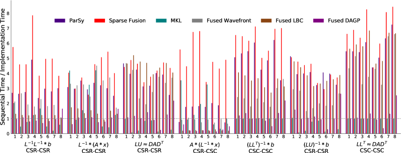
Figure 6. Performance of different implementations shown with speedup from dividing baseline time by implementation time.

fusion executor performance.

Sparse Fusion’s Performance. Figure 6 shows the performance of the fused code from sparse fusion, the unfused implementation from ParSy and MKL, and the fused wavefront, fused LBC, and fused DAGP implementations. All execution times are normalized over a baseline. The baseline is obtained by running each kernel individually with a sequential implementation. The floating point operations per second (FLOP/s) for each implementation can be obtained by multiplying the baseline FLOP/s from Table 3 with the speedups in Figure 6. The sparse fusion’s fused code is on average 1.6$\times$ faster than ParSy’s executor code and 5.1$\times$ faster than MKL across all kernel combinations. Even though sparse fusion is on average 11.5$\times$ faster than MKL for ILU0-TRSV, since ILU0 only has a sequential implementation in MKL, the speedup of this kernel combination is excluded from the average speedups. The fused code from sparse fusion is on average 2.5$\times$, 5.1$\times$, and 7.2$\times$ faster than in order fused wavefront, fused LBC, and fused DAGP. Obtained speedups of sparse fusion over ParSy (the fastest unfused implementation) for SpILU0-SpTRSV and SpIC0-SpTRSV is lower than other kernel combinations. Because SpIC0 and SpILU0 have a high execution time, when combined with others sparse kernels with a noticeably lower execution time, the realized speedup from fusion will not be significant.

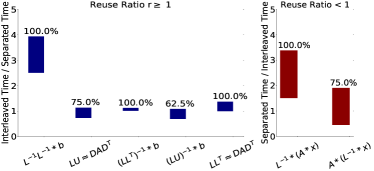
Figure 7. The range of speedup for all matrices achieved as a result of using interleaved packing vs. separated packing. The labels on bars show how often the choice of packing strategy made by sparse fusion leads to performance improvement.

Profiling overall.

Locality in Sparse Fusion. Figure 7 shows the efficiency of the two packing strategies to improve locality. The effect of the packing strategy is shown for kernel combinations with a reuse ratio smaller and larger than one as shown in Table 2. Kernel combinations 1, 3, 5, 6, and 7 share the sparse matrix $L$ and thus have a reuse ratio larger than one while combination 2 and 4 only share vector $y$ leading to a reuse ratio lower than one. Figure 7 shows the range of speedup over all matrices for the selected packing strategy versus the other other packing method for each combination. As shown, the selected packing strategy in sparse fusion improves the performance in 88% of kernel combinations and matrices and provides 1-3.9$\times$ improvement in both categories.

Figure 8 shows the average memory access latency (Hennessy and Patterson, 2017) of sparse fusion, the fastest unfused implementation (ParSy), and the fastest fused partitioning-based implementation (Fused LBC) for all kernel combinations normalized over the ParSy average memory access latency (shown for matrix bone010 as example, other matrices exhibit similar behavior). The average memory access latency is used as a proxy for locality and is computed using the number of accesses to L1, LLC, and TLB measured with PAPI performance counters (Terpstra et al., 2010).

For kernels 1, 3, 5, 6, and 7 where the reuse ratio is larger than one, the memory access latency of ParSy is on average 1.3$\times$ larger than that of sparse fusion. Because of their high reuse ratio, these kernels benefit from optimizing locality between kernels made possible via interleaved packing. ParSy optimizes locality in each kernel individually. When applied to the joint DAG, LBC can potentially improve the temporal locality between kernels and thus there is only a small gap between the memory access latency of sparse fusion and that of fused LBC. For kernels 2 and 4 where the reuse ratio is smaller than one, the gap between the memory access latency of sparse fusion and fused LBC is larger than the gap between the memory access latency of sparse fusion and ParSy. Sparse fusion and ParSy both improve data locality within each kernel for these kernel combinations.

Load Balance and Synchronization in Sparse Fusion. Figure 8 shows the OpenMP potential gain (Software, 2018) of sparse fusion, ParSy, and Fused LBC for all kernel combinations normalized over ParSy’s potential gain (shown for matrix bone010 as example, but all other matrices in Table 1 follow similar behavior.) The OpenMP potential gain is a metric in Vtune (Zone, [n.d.]) that shows the total parallelism overhead, e.g. wait-time due to load imbalance and synchronization overhead, divided by the number of threads. This metric is used to measure the load imbalance and synchronization overhead in ParSy, fused LBC, and sparse fusion.

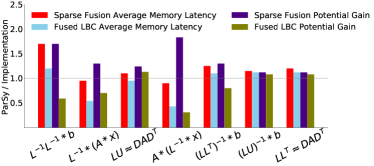
Figure 8. Average memory access time and the OpenMP potential gain for matrix bone010. The legends show the implementation, values are normalized over ParSy.

Profiling.

Kernel combinations 2 and 4 have slack vertices that provide opportunities to balance workloads. For example, for matrices shown in Table 1, between 35-76% vertices can be slacked thus the potential gain balance of ParSy is 1.6$\times$ larger than sparse fusion and 2.4$\times$ lower than fused LBC. ParSy can only improve load balance using the workloads of an individual kernel. As shown in Figure 1, for the kernel combination 5, the joint DAG has a small number of parallel iterations in final wavefronts that makes the final s-partitions of the LBC fused implementation imbalanced (a similar trend exists for kernel combination 6). For these kernel combinations, the code from sparse fusion has on average 33% fewer synchronization barriers compared to ParSy due to merging. For kernel combinations 1, 2, 3, 4, and 7 the potential gain in sparse fusion is 1.3$\times$ less than that of ParSy. Merging in sparse fusion reduces the number of synchronizations in the fused code on average 50% compared to that of ParSy.

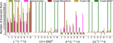
Figure 9. The number of executor runs to amortize inspector cost. Values are clipped between -5 and 80. (lower is better)

fusion inspector performance.

Inspector Time. Figure 9 shows the number of times that the executor should run to amortize the cost of inspection for implementations that have an inspector. For space only combinations 1, 3, 4, and 5 are shown, others follow the same trend. The number of executor runs (NER) that amortize the cost of inspector for an implementation is calculated using
$\frac{\>\>Inspector\>\>Time}{Baseline\>Time-\>\>Executor\>\>Time}$. The baseline time is obtained by running each kernel individually with a sequential implementation, the inspector and executor times belong to the specific implementation. The fused LBC implementation has a NER of 3.1-745. The high inspection time is because of the high cost of converting the joint DAG into a chordal DAG, typically consuming 64% of its inspection time. The NER of the fused DAGP implementation is either negative or higher than 80. The fused wavefront implementation sometimes has a negative NER because the executor time is slower than the baseline time. As shown, sparse fusion and fused wavefront have the lowest NER amongst all implementations. Sparse fusion’s low inspection time is due to pairing strategies that enable partitioning one DAG at a time. Kernel combinations such as, SpIC0-TRSV and SpILU0-TRSV only need one iteration to amortize the inspection time and SpTRSV-SpMV, SpTRSV-SptRSV, and SpMV-SpTRSV need between 11-50 iterations. Sparse kernel combinations are routinely used in iterative solvers in scientific applications. Even with preconditioning, these solvers typically converge to an accurate solution after ten of thousands of iterations (Benzi et al., 2000; Kershaw, 1978; Papadrakakis and Bitoulas, 1993), hence amortizing the overhead of inspection.

5. Related work

Parallel implementations of individual sparse matrix kernels exist in both highly-optimized libraries (Hénon et al., 2002; Li, 2005) and inspector-executor approaches (Cheshmi et al., 2017; Mohammadi et al., 2019; Strout et al., 2018). Some libraries such as MKL (Wang et al., 2014), and code generators such as Taichi (Hu et al., 2019) and TACO (Fredrik Kjolstad and Amarasinghe, 2017) provide optimizations for a range of sparse matrix kernels, while others provide optimizations for a specific sparse kernel. For example, the sparse triangular solve has been optimized in (Li and Saad, 2013; Naumov, 2011; Wang et al., 2018; Vuduc et al., 2002; Totoni et al., 2014; Yılmaz et al., 2020; Park et al., 2014; Picciau et al., 2016; Saltz, 1990), optimizations of sparse matrix-vector multiply are available in (Williams et al., 2009; Kamin et al., 2014; Merrill and Garland, 2016; Li et al., 2013; Ashari et al., 2014; Liu et al., 2018), and LU and Cholesky factorization have been optimized in SuperLU (Li, 2005) and Pastix (Hénon et al., 2002).

Inspector-executor frameworks commonly use wavefront parallelism (Venkat et al., 2016; Rauchwerger et al., 1995; Zhuang et al., 2009; Strout et al., 2002; Naumov, 2011; Govindarajan and Anantpur, 2013) to parallelize sparse matrix computations with loop-carried dependencies. Recently, task coarsening approaches such as LBC (Cheshmi et al., 2018) and DAGP (Herrmann et al., 2019) coarsen wavefronts and thus generate code that is optimized for parallelism, load balance, and locality. While available approaches can provide efficient optimizations for sparse kernels with or without loop-carried dependencies, they can only optimize sparse kernels individually.

A number of libraries and inspector-executor frameworks provide parallel implementations of fused sparse kernels with no loop-carried dependencies such as, two or more SpMV kernels (Hoemmen et al., 2010; MehriDehnavi et al., 2013; Mohiyuddin et al., 2009; Aliaga et al., 2015; Rupp et al., 2016) or SpMV and dot products (Zhuang and Casas, 2017b; Dehnavi et al., 2011; Aliaga et al., 2015; Ghysels and Vanroose, 2014; Agullo et al., 2009; Rupp et al., 2016). The formulation of $s$-step Krylov solvers (Carson, 2015) has enabled iterations of iterative solvers to be interleaved and hence multiple SpMV kernels are optimized simultaneously via replicating computations to minimize communication costs (Hoemmen et al., 2010; MehriDehnavi et al., 2013; Mohiyuddin et al., 2009; Soori et al., 2018). Sparse tiling (Strout et al., 2003; Krieger et al., 2013; Strout et al., 2014, 2002; Strout et al., 2004) is an inspector executor approach that uses manually written inspectors (Strout et al., 2003, 2004) to group iteration of different loops of a specific kernel such as Gauss-Seidel (Strout et al., 2004) and Moldyn (Strout et al., 2003) and is generalized for parallel loops without loop-carried dependencies (Strout et al., 2014; Krieger et al., 2013). Sparse fusion optimizes combinations of sparse kernels where at least one of the kernels has loop-carried dependencies.

6. Conclusion

We present sparse fusion and demonstrate how it improves parallelism, load balance, and data locality in sparse matrix combinations compared to when sparse kernels are optimized separately. Sparse fusion inspects the DAGs of the input sparse kernels and uses the MSP algorithm to balance the workload between wavefronts and determine whether to optimize data locality for within or between the kernels. Sparse fusion’s generated code outperforms state-of-the-art implementations for sparse matrix optimizations. In future work, we plan to investigate strategies that select the most profitable loops to be fused to support the fusion of more than two loops.

- (1)
- Agullo et al. (2009) Emmanuel Agullo, Jim Demmel, Jack Dongarra, Bilel Hadri, Jakub Kurzak, Julien Langou, Hatem Ltaief, Piotr Luszczek, and Stanimire Tomov. 2009. Numerical linear algebra on emerging architectures: The PLASMA and MAGMA projects. In Journal of Physics: Conference Series, Vol. 180. IOP Publishing, 012037.
- Aliaga et al. (2015) José I Aliaga, Joaquín Pérez, and Enrique S Quintana-Ortí. 2015. Systematic fusion of CUDA kernels for iterative sparse linear system solvers. In European Conference on Parallel Processing. Springer, 675–686.
- Ashari et al. (2014) Arash Ashari, Naser Sedaghati, John Eisenlohr, Srinivasan Parthasarath, and P Sadayappan. 2014. Fast sparse matrix-vector multiplication on GPUs for graph applications. In SC’14: Proceedings of the International Conference for High Performance Computing, Networking, Storage and Analysis. IEEE, 781–792.
- Benzi et al. (2000) Michele Benzi, Jane K Cullum, and Miroslav Tuma. 2000. Robust approximate inverse preconditioning for the conjugate gradient method. SIAM Journal on Scientific Computing 22, 4 (2000), 1318–1332.
- Boyd et al. (2004) Stephen Boyd, Stephen P Boyd, and Lieven Vandenberghe. 2004. Convex optimization. Cambridge university press.
- Carson (2015) Erin Claire Carson. 2015. Communication-avoiding Krylov subspace methods in theory and practice. Ph.D. Dissertation. UC Berkeley.
- Cheshmi et al. (2017) Kazem Cheshmi, Shoaib Kamil, Michelle Mills Strout, and Maryam Mehri Dehnavi. 2017. Sympiler: transforming sparse matrix codes by decoupling symbolic analysis. In Proceedings of the International Conference for High Performance Computing, Networking, Storage and Analysis. 1–13.
- Cheshmi et al. (2018) Kazem Cheshmi, Shoaib Kamil, Michelle Mills Strout, and Maryam Mehri Dehnavi. 2018. ParSy: inspection and transformation of sparse matrix computations for parallelism. In SC18: International Conference for High Performance Computing, Networking, Storage and Analysis. IEEE, 779–793.
- Cheshmi et al. (2020) Kazem Cheshmi, Danny M Kaufman, Shoaib Kamil, and Maryam Mehri Dehnavi. 2020. NASOQ: numerically accurate sparsity-oriented QP solver. ACM Transactions on Graphics (TOG) 39, 4 (2020), 96–1.
- Chow and Patel (2015) Edmond Chow and Aftab Patel. 2015. Fine-grained parallel incomplete LU factorization. SIAM journal on Scientific Computing 37, 2 (2015), C169–C193.
- Davis (2006) Timothy A Davis. 2006. Direct methods for sparse linear systems. SIAM.
- Davis and Hu (2011) Timothy A Davis and Yifan Hu. 2011. The University of Florida sparse matrix collection. ACM Transactions on Mathematical Software (TOMS) 38, 1 (2011), 1.
- Dehnavi et al. (2011) Maryam Mehri Dehnavi, David M Fernández, and Dennis Giannacopoulos. 2011. Enhancing the performance of conjugate gradient solvers on graphic processing units. IEEE Transactions on Magnetics 47, 5 (2011), 1162–1165.
- Fredrik Kjolstad and Amarasinghe (2017) David Lugato Fredrik Kjolstad, Shoaib Kamil Stephen Chou and Saman Amarasinghe. 2017. The Tensor Algebra Compiler. Technical Report. Massachusetts Institute of Technology.
- Ghysels and Vanroose (2014) Pieter Ghysels and Wim Vanroose. 2014. Hiding global synchronization latency in the preconditioned conjugate gradient algorithm. Parallel Comput. 40, 7 (2014), 224–238.
- Govindarajan and Anantpur (2013) R Govindarajan and Jayvant Anantpur. 2013. Runtime dependence computation and execution of loops on heterogeneous systems. In Proceedings of the 2013 IEEE/ACM International Symposium on Code Generation and Optimization (CGO). IEEE Computer Society, 1–10.
- Grigori and Moufawad (2015) Laura Grigori and Sophie Moufawad. 2015. Communication avoiding ILU0 preconditioner. SIAM Journal on Scientific Computing 37, 2 (2015), C217–C246.
- Hennessy and Patterson (2017) John L Hennessy and David A Patterson. 2017. Computer architecture: a quantitative approach. Elsevier.
- Hénon et al. (2002) Pascal Hénon, Pierre Ramet, and Jean Roman. 2002. PASTIX: a high-performance parallel direct solver for sparse symmetric positive definite systems. Parallel Comput. 28, 2 (2002), 301–321.
- Herrmann et al. (2019) Julien Herrmann, M Yusuf Ozkaya, Bora Uçar, Kamer Kaya, and Ümit VV Çatalyürek. 2019. Multilevel algorithms for acyclic partitioning of directed acyclic graphs. SIAM Journal on Scientific Computing 41, 4 (2019), A2117–A2145.
- Hoemmen et al. (2010) Mark Frederick Hoemmen et al. 2010. Communication-avoiding Krylov subspace methods. (2010).
- Hu et al. (2019) Yuanming Hu, Tzu-Mao Li, Luke Anderson, Jonathan Ragan-Kelley, and Frédo Durand. 2019. Taichi: A Language for High-Performance Computation on Spatially Sparse Data Structures. ACM Trans. Graph. 38, 6, Article 201 (Nov. 2019), 16 pages. https://doi.org/10.1145/3355089.3356506
- Kamin et al. (2014) Sam Kamin, María Jesús Garzarán, Barış Aktemur, Danqing Xu, Buse Yılmaz, and Zhongbo Chen. 2014. Optimization by runtime specialization for sparse matrix-vector multiplication. In ACM SIGPLAN Notices, Vol. 50. ACM, 93–102.
- Karypis and Kumar (1998) George Karypis and Vipin Kumar. 1998. A software package for partitioning unstructured graphs, partitioning meshes, and computing fill-reducing orderings of sparse matrices. University of Minnesota, Department of Computer Science and Engineering, Army HPC Research Center, Minneapolis, MN (1998).
- Kershaw (1978) David S Kershaw. 1978. The incomplete Cholesky-conjugate gradient method for the iterative solution of systems of linear equations. Journal of computational physics 26, 1 (1978), 43–65.
- Krieger et al. (2013) Christopher D Krieger, Michelle Mills Strout, Catherine Olschanowsky, Andrew Stone, Stephen Guzik, Xinfeng Gao, Carlo Bertolli, Paul HJ Kelly, Gihan Mudalige, Brian Van Straalen, et al. 2013. Loop chaining: A programming abstraction for balancing locality and parallelism. In 2013 IEEE International Symposium on Parallel & Distributed Processing, Workshops and Phd Forum. IEEE, 375–384.
- Li et al. (2013) Jiajia Li, Guangming Tan, Mingyu Chen, and Ninghui Sun. 2013. SMAT: an input adaptive auto-tuner for sparse matrix-vector multiplication. In Proceedings of the 34th ACM SIGPLAN conference on Programming language design and implementation. 117–126.
- Li and Saad (2013) Ruipeng Li and Yousef Saad. 2013. GPU-accelerated preconditioned iterative linear solvers. The Journal of Supercomputing 63, 2 (2013), 443–466.
- Li (2005) Xiaoye S Li. 2005. An overview of SuperLU: Algorithms, implementation, and user interface. ACM Transactions on Mathematical Software (TOMS) 31, 3 (2005), 302–325.
- Liu et al. (2018) Changxi Liu, Biwei Xie, Xin Liu, Wei Xue, Hailong Yang, and Xu Liu. 2018. Towards efficient SpMV on sunway manycore architectures. In Proceedings of the 2018 International Conference on Supercomputing. 363–373.
- MehriDehnavi et al. (2013) M. MehriDehnavi, Y. El-Kurdi, J. Demmel, and D. Giannacopoulos. 2013. Communication-Avoiding Krylov Techniques on Graphic Processing Units. IEEE Transactions on Magnetics 49, 5 (2013), 1749–1752. https://doi.org/10.1109/TMAG.2013.2244861
- Merrill and Garland (2016) Duane Merrill and Michael Garland. 2016. Merge-based parallel sparse matrix-vector multiplication. In Proceedings of the International Conference for High Performance Computing, Networking, Storage and Analysis. IEEE Press, 58.
- Mohammadi et al. (2019) Mahdi Soltan Mohammadi, Tomofumi Yuki, Kazem Cheshmi, Eddie C Davis, Mary Hall, Maryam Mehri Dehnavi, Payal Nandy, Catherine Olschanowsky, Anand Venkat, and Michelle Mills Strout. 2019. Sparse computation data dependence simplification for efficient compiler-generated inspectors. In Proceedings of the 40th ACM SIGPLAN Conference on Programming Language Design and Implementation. 594–609.
- Mohiyuddin et al. (2009) M. Mohiyuddin, M. Hoemmen, J. Demmel, and K. Yelick. 2009. Minimizing communication in sparse matrix solvers. In Proceedings of the Conference on High Performance Computing Networking, Storage and Analysis. 1–12. https://doi.org/10.1145/1654059.1654096
- Naumov (2011) Maxim Naumov. 2011. Parallel solution of sparse triangular linear systems in the preconditioned iterative methods on the GPU. NVIDIA Corp., Westford, MA, USA, Tech. Rep. NVR-2011 1 (2011).
- Papadrakakis and Bitoulas (1993) M Papadrakakis and N Bitoulas. 1993. Accuracy and effectiveness of preconditioned conjugate gradient algorithms for large and ill-conditioned problems. Computer methods in applied mechanics and engineering 109, 3-4 (1993), 219–232.
- Park et al. (2014) Jongsoo Park, Mikhail Smelyanskiy, Narayanan Sundaram, and Pradeep Dubey. 2014. Sparsifying Synchronization for High-Performance Shared-Memory Sparse Triangular Solver. In Proceedings of the 29th International Conference on Supercomputing - Volume 8488 (ISC 2014). Springer-Verlag New York, Inc., New York, NY, USA, 124–140.
- Picciau et al. (2016) A. Picciau, G. E. Inggs, J. Wickerson, E. C. Kerrigan, and G. A. Constantinides. 2016. Balancing Locality and Concurrency: Solving Sparse Triangular Systems on GPUs. In 2016 IEEE 23rd International Conference on High Performance Computing (HiPC). 183–192.
- Rauchwerger et al. (1995) Lawrence Rauchwerger, Nancy M Amato, and David A Padua. 1995. Run-time methods for parallelizing partially parallel loops. In Proceedings of the 9th international conference on Supercomputing. 137–146.
- Rupp et al. (2016) Karl Rupp, Philippe Tillet, Florian Rudolf, Josef Weinbub, Andreas Morhammer, Tibor Grasser, Ansgar Jungel, and Siegfried Selberherr. 2016. ViennaCL—linear algebra library for multi-and many-core architectures. SIAM Journal on Scientific Computing 38, 5 (2016), S412–S439.
- Saad (2003) Yousef Saad. 2003. Iterative methods for sparse linear systems. SIAM.
- Saad and Malevsky (1995) Yousef Saad and Andrei V Malevsky. 1995. P-Sparslib: a portable library of distributed memory sparse iterative solvers. In Proceedings of Parallel Computing Technologies (PaCT-95), 3-rd international conference, St. Petersburg. Citeseer.
- Saltz (1990) Joel H. Saltz. 1990. Aggregation methods for solving sparse triangular systems on multiprocessors. SIAM J. Sci. Statist. Comput. 11, 1 (1990), 123–144.
- Software (2018) Intel Software. 2018. OpenMP potential gain definition in intel VTune. https://software.intel.com/content/www/us/en/develop/documentation/vtune-help/top/reference/cpu-metrics-reference/openmp-potential-gain.html
- Soori et al. (2018) Saeed Soori, Aditya Devarakonda, Zachary Blanco, James Demmel, Mert Gurbuzbalaban, and Maryam Mehri Dehnavi. 2018. Reducing communication in proximal Newton methods for sparse least squares problems. In Proceedings of the 47th International Conference on Parallel Processing. 1–10.
- Stellato et al. (2020) Bartolomeo Stellato, Goran Banjac, Paul Goulart, Alberto Bemporad, and Stephen Boyd. 2020. OSQP: An operator splitting solver for quadratic programs. Mathematical Programming Computation (2020), 1–36.
- Strout et al. (2003) Michelle Mills Strout, Larry Carter, and Jeanne Ferrante. 2003. Compile-time composition of run-time data and iteration reorderings. In Proceedings of the ACM SIGPLAN 2003 conference on Programming language design and implementation. 91–102.
- Strout et al. (2002) Michelle Mills Strout, Larry Carter, Jeanne Ferrante, Jonathan Freeman, and Barbara Kreaseck. 2002. Combining performance aspects of irregular gauss-seidel via sparse tiling. In International Workshop on Languages and Compilers for Parallel Computing. Springer, 90–110.
- Strout et al. (2004) Michelle Mills Strout, Larry Carter, Jeanne Ferrante, and Barbara Kreaseck. 2004. Sparse tiling for stationary iterative methods. The International Journal of High Performance Computing Applications 18, 1 (2004), 95–113.
- Strout et al. (2018) Michelle Mills Strout, Mary Hall, and Catherine Olschanowsky. 2018. The sparse polyhedral framework: Composing compiler-generated inspector-executor code. Proc. IEEE 106, 11 (2018), 1921–1934.
- Strout et al. (2014) Michelle Mills Strout, Fabio Luporini, Christopher D Krieger, Carlo Bertolli, Gheorghe-Teodor Bercea, Catherine Olschanowsky, J Ramanujam, and Paul HJ Kelly. 2014. Generalizing run-time tiling with the loop chain abstraction. In 2014 IEEE 28th International Parallel and Distributed Processing Symposium. IEEE, 1136–1145.
- Terpstra et al. (2010) Dan Terpstra, Heike Jagode, Haihang You, and Jack Dongarra. 2010. Collecting performance data with PAPI-C. In Tools for High Performance Computing 2009. Springer, 157–173.
- Totoni et al. (2014) Ehsan Totoni, Michael T Heath, and Laxmikant V Kale. 2014. Structure-adaptive parallel solution of sparse triangular linear systems. Parallel Comput. 40, 9 (2014), 454–470.
- Venkat et al. (2016) Anand Venkat, Mahdi Soltan Mohammadi, Jongsoo Park, Hongbo Rong, Rajkishore Barik, Michelle Mills Strout, and Mary Hall. 2016. Automating wavefront parallelization for sparse matrix computations. In Proceedings of the International Conference for High Performance Computing, Networking, Storage and Analysis. IEEE Press, 41.
- Vuduc et al. (2002) Richard Vuduc, Shoaib Kamil, Jen Hsu, Rajesh Nishtala, James W Demmel, and Katherine A Yelick. 2002. Automatic performance tuning and analysis of sparse triangular solve. ICS.
- Wang et al. (2014) Endong Wang, Qing Zhang, Bo Shen, Guangyong Zhang, Xiaowei Lu, Qing Wu, and Yajuan Wang. 2014. Intel math kernel library. In High-Performance Computing on the Intel® Xeon Phi™. Springer, 167–188.
- Wang et al. (2018) Xinliang Wang, Wei Xue, Weifeng Liu, and Li Wu. 2018. swSpTRSV: a fast sparse triangular solve with sparse level tile layout on sunway architectures. In Proceedings of the 23rd ACM SIGPLAN Symposium on Principles and Practice of Parallel Programming. ACM, 338–353.
- Williams et al. (2009) Samuel Williams, Leonid Oliker, Richard Vuduc, John Shalf, Katherine Yelick, and James Demmel. 2009. Optimization of sparse matrix–vector multiplication on emerging multicore platforms. Parallel Comput. 35, 3 (2009), 178–194.
- Yılmaz et al. (2020) Buse Yılmaz, Buğrra Sipahioğrlu, Najeeb Ahmad, and Didem Unat. 2020. Adaptive Level Binning: A New Algorithm for Solving Sparse Triangular Systems. In Proceedings of the International Conference on High Performance Computing in Asia-Pacific Region. 188–198.
- Zhuang and Casas (2017a) Sicong Zhuang and Marc Casas. 2017a. Iteration-fusing conjugate gradient. In Proceedings of the International Conference on Supercomputing. 1–10.
- Zhuang and Casas (2017b) Sicong Zhuang and Marc Casas. 2017b. Iteration-Fusing Conjugate Gradient. In Proceedings of the International Conference on Supercomputing (Chicago, Illinois) (ICS ’17). Association for Computing Machinery, New York, NY, USA, Article 21, 10 pages. https://doi.org/10.1145/3079079.3079091
- Zhuang et al. (2009) Xiaotong Zhuang, Alexandre E Eichenberger, Yangchun Luo, Kevin O’Brien, and Kathryn O’Brien. 2009. Exploiting parallelism with dependence-aware scheduling. In Parallel Architectures and Compilation Techniques, 2009. PACT’09. 18th International Conference on. IEEE, 193–202.
- Zone ([n.d.]) Intel Developer Zone. [n.d.]. Intel VTune Amplifier, 2017. Documentation at the URL: https://software.intel.com/en-us/intel-vtune-amplifier-xe-support/documentation ([n. d.]).