The JCMT BISTRO Survey: Evidence for Pinched Magnetic Fields in Quiescent Filaments of NGC 1333

Abstract

We investigate the internal 3D magnetic structure of dense interstellar filaments within NGC 1333 using polarization data at $850~{}\mu\mathrm{m}$ from the B-fields In STar-forming Region Observations survey at the James Clerk Maxwell Telescope. Theoretical models predict that the magnetic field lines in a filament will tend to be dragged radially inward (i.e., pinched) toward the central axis due to the filament’s self-gravity. We study the cross-sectional profiles of the total intensity (I) and polarized intensity (PI) of dust emission in four segments of filaments unaffected by local star formation that are expected to retain a pristine magnetic field structure. We find that the filaments’ FWHMs in PI are not the same as those in I, with two segments being appreciably narrower in PI (FWHM ratio $\simeq 0.7$–0.8) and one segment being wider (FWHM ratio $\simeq 1.3$). The filament profiles of the polarization fraction (P) do not show a minimum at the spine of the filament, which is not in line with an anticorrelation between P and I normally seen in molecular clouds and protostellar cores. Dust grain alignment variation with density cannot reproduce the observed P distribution. We demonstrate numerically that the I and PI cross-sectional profiles of filaments in magnetohydrostatic equilibrium will have differing relative widths depending on the viewing angle. The observed variations of FWHM ratios in NGC 1333 are therefore consistent with models of pinched magnetic field structures inside filaments, and especially if they are magnetically near-critical or supercritical.

1 Introduction

It is widely recognized that filaments in the interstellar medium (ISM) play an essential role in the star formation process (e.g., André et al., 2014). Theoretical studies indicate that the magnetic field (B-field hereafter) contributes to the evolution of these filaments (e.g., Hennebelle & Inutsuka, 2019). It is, therefore, crucial to observe the B-field in quiescent filaments before the onset of star formation to understand their dynamical importance in shaping these ubiquitous structures.

Specifically, the plane-of-sky (POS) component of the B-field can be traced with polarimetric observations of the thermal continuum emission from interstellar dust particles (e.g., Hildebrand, 1988). Aspherical dust particles irradiated by incoming radiation fields are spun up by radiative alignment torques (RATs; Lazarian & Hoang, 2007), which align their rotation axes parallel to the ambient B-field direction. As a result, the thermal emission from so-aligned dust particles is polarized, and the polarization angle is perpendicular to the POS-projected B-field (Stein, 1966; Hildebrand, 1988).

For a uniform B-field along the line of sight (LOS), the polarized intensity (PI) and, similarly, the polarization fraction (P) relative to the total intensity (I) depend on the degree of alignment of the dust particles. Assuming that the alignment is produced by the surrounding radiation field (i.e., RAT theory), P will become smaller in high gas density regions shielded from this radiation (Hoang et al., 2021).

Also, P has a dependence on the viewing angle of the B-field. If the B-field is highly inclined relative to the POS, P can be lower, since the rotation axes of aspherical dust particles become nearly parallel to the LOS in such arrangements. Moreover, the B-field itself can be complicated within the observational beam or along the LOS by, e.g., gas turbulent motions. Unresolved polarization structures will result in depolarization, as multiple position angles within the telescope beam cancel out and reduce the observed P (geometric depolarization).

In the Perseus molecular cloud, NGC 1333 is an active star-forming region with a complex network of massive (gravitationally supercritical) filaments (e.g., Hacar et al., 2017). Doi et al. (2020, hereafter Paper I) made a polarimetry study of NGC 1333 as a part of the B-fields In STar-forming Region Observations (BISTRO) survey using the Sub-millimeter Common-User Bolometer Array 2 (SCUBA-2) camera and its polarimeter (POL-2) on the James Clerk Maxwell Telescope (JCMT). The distance to this area is estimated to be $\simeq 300$ pc (Zucker et al., 2018, 2019; Pezzuto et al., 2021), giving a spatial resolution of 0.02 pc for the $14\arcsec.1$ JCMT beam (FWHM; Dempsey et al., 2013) at $850~{}\mu\mathrm{m}$. With this high spatial resolution, Paper I spatially resolved the polarized emission from these filaments for the first time. In this paper, we take advantage of these same data to investigate the 3D morphology of the B-field inside several quiescent massive filaments.

This paper is organized as follows. In Section 2, we outline our data reduction, with full details given in Paper I, together with our estimation of the cross-sectional profiles of filaments in I, PI, and P. In Section 3, we describe the characteristics of the estimated cross-sectional profiles. In Section 4, we compare our observations with a magnetohydrostatic simulation (Tomisaka, 2014) and investigate the 3D B-field morphology inside the filament. We discuss the assumptions and caveats of this work in Section 5. In Section 6, we conclude with a summary of our results.

2 Observations and Methods

We use the same polarimetry data as in Paper I (see that paper for full details of the observations and data analysis). The observation covers the main part ($\sim 1.5\mathrm{pc}\times 2.0\mathrm{pc}$) of NGC 1333, and an intricate network of filaments with a column density above $\sim 10^{23}~{}\mathrm{H_{2}~{}cm^{-2}}$ is detected in I and PI with a good signal-to-noise ratio (S/N) of $I/\delta I\geqslant 10$ and $\mathrm{PI}/\delta\mathrm{PI}\geqslant 3$. A central cutout of the observation is shown in Figure 1. We check the I and PI sensitivity as a function of the spatial frequency by estimating the spatial power spectra of I and PI along the blue dashed line in Figure 1. We confirm that two observations trace the small-scale structure comparable to the filament width with equal sensitivity (Appendix A).

In Paper I, we identified five filaments in the observed region. Here we obtain cross-sectional profiles of these filaments for locations that satisfy each of the following conditions.

1. The S/N of the PI emission $\mathrm{PI}/\delta\mathrm{PI}\geqslant 3$ over more than three contiguous observational beams.

2. No star formation activity is found in its vicinity (see Figure 1 and Appendix C). Thus, the radiation and dynamic interaction via, e.g., bipolar outflows from active star-forming regions that may affect the filament profile is expected to be negligible.

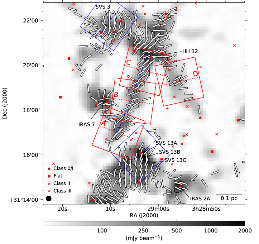
Figure 1: Four NGC 1333 positions where we measure cross sections of filaments. The red dotted lines are the positions of cross sections shown in Figure 2. The red boxes correspond to the smoothed maps we show in Figure A.2 (see text). The blue dotted lines with blue boxes are the locations of the example filament profiles for the active regions for comparison, shown in Figures A.4 and 5. These profiles are briefly described in Section 5. The blue dashed line is the position where we estimate spatial power spectra of I and PI to confirm that we observe small-scale structures in these emissions with equal sensitivities. The gray scale is the $850~{}\mu\mathrm{m}$ Stokes $I$ map, and black contours indicate $\mathrm{PI}/\delta\mathrm{PI}\geqslant 5$ (Paper I). White line segments indicate the POS magnetic field orientations (Paper I). We plot the magnetic field orientations for the data points with $I\geqslant 25~{}\mathrm{mJy~{}beam^{-1}}$ and $\mathrm{PI}/\delta\mathrm{PI}\geqslant 3$. Note that the length of the line segments has been normalized to show only the orientation of the magnetic field. The positions of the main infrared sources indicated in the figure are taken from Sandell & Knee (2001). Red symbols are embedded YSOs ($A_{V}\geqslant 3$ mag; Evans et al., 2009; Young et al., 2015). Circles: class 0/I; squares: flat, crosses: class II, stars: class III. The JCMT beam ($14\arcsec.1$) is shown in the lower left corner. A reference scale for 0.1 pc is shown, for which we assume the distance to the source to be 300 pc (Ortiz-León et al., 2018; Zucker et al., 2018; see Paper I).

We identify four filament segments, A, B, C, and D, in Figure 1 that fulfill these conditions. All but segment D are in fact identified with $\mathrm{PI}/\delta\mathrm{PI}\geqslant 5$. Segments B and C are bridged by radiation with $\mathrm{PI}/\delta\mathrm{PI}\geqslant 3$, but we treat them as two independent regions because of their clear separation, which can be seen in the contour with $\mathrm{PI}/\delta\mathrm{PI}=5$ (Figure 1).

We measure the Stokes I, Q, and U intensities in each segment in the same way as in Paper I. Additionally, we smooth the data in the direction along the segment five times the beam to boost the S/N by a factor of $\sqrt{5}$. See Appendix B and Figure A.2 for the details of the derivation method and the resulting intensity maps.

The positions over which we estimate the filament cross-sectional profiles are shown as horizontal dotted lines in Figure 1. For segment A, the dotted line correspond to the peak in PI intensity. For segment B, the PI profile of the peak position shows the contribution of another peak visible in the upper right part of the PI map (the southern extension of segment C; see Figures 1 and A.2), resulting in a relatively large fitting error. Hence, we choose a location one beam south of the PI peak to avoid the influence of this additional peak to achieve a Gaussian fit with reasonable accuracy. The difference in fitting results between these two positions is not statistically significant, and this position shift does not affect the following discussion. For segment C, the PI and I intensities increase continuously toward HH12 in the north, so we set the position of C near the middle of the filament to also exclude a class 0/I young stellar object (YSO; J032901.56+312020.6; see Figure A.2) from the evaluation of the cross section. For segment D, we ignore one class II YSO (J032856.12+311908.4; see Figure A.2) as a foreground source because it has an estimated $A_{V}=0$ mag (Evans et al., 2009), and the source probably does not affect the filament’s internal structure. We thus set the position of D at the peak in PI intensity.

The projected distances to the neighboring YSOs from the centers of the cross sections are $\geqslant 0.05$ pc. Stellar flux from a classical T Tauri star at 0.05 pc corresponds to $\sim 0.03$–0.3 of the average interstellar radiation field (France et al., 2014). The flux will be smaller if there is absorption between the star and the filament. Thus, we judge that the radiation from the neighboring YSOs on the selected filament segments is negligible. We further check the dust temperature distribution (Pezzuto et al., 2021) and find that both embedded heating source(s) and nonuniform external heating from nearby sources are negligible (Appendix C). In addition, there is no signs of outflows from YSOs in these filament segments (Dionatos et al., 2020). Also, we find no indication of interaction between outflows and filaments in the observed B-field morphology (Paper I).

3 Results

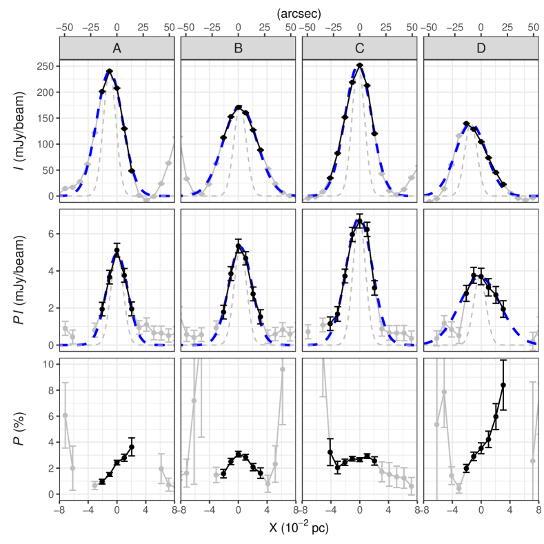
Figure 2: Cross-sectional profiles of the selected NGC 1333 filamentary structures. The X-axis points west, and the positions of the cross sections are indicated as red dotted lines in Figure 1. See Appendix B for the intensity and its error estimations. We performed Gaussian fits using $\mathrm{PI}/\delta\mathrm{PI}\geq 3$ data, displayed in black in the cross-sectional profiles, and we do not use the data with $\mathrm{PI}/\delta\mathrm{PI}<3$, shown in gray for the fitting (Appendix B). The fitting results are shown as blue dashed lines in those panels. The gray dashed lines are the beam profile of the observation ($\mathrm{FWHM}=14\arcsec.1$) for comparison. Note that the data points in each cross section are plotted twice per beam, while fitting is performed using only one point per beam.

We show the measured cross-sectional profiles of I, PI, and P of the filament segments in Figure 2. We estimate the FWHM of the I and PI profiles with $\mathrm{PI}/\delta\mathrm{PI}\geqslant 3$ (black symbols in the figure) by fitting 1D Gaussian profiles (see Appendix B for the details), which we show as blue dashed lines. The results are summarized in Table 1.

Table 1: Estimated FWHM Values

Segment	$\mathrm{FWHM}(I)$	$\mathrm{FWHM}(\mathrm{PI})$	$\dfrac{\mathrm{FWHM}(\mathrm{PI})}{\mathrm{FWHM}(I)}$
	(pc)	(pc)
A	$0.043\pm 0.001$	$0.034\pm 0.002$	$0.81\pm 0.04$
	($0.036\pm 0.001$)	($0.027\pm 0.002$)	($0.74\pm 0.05$)
B	$0.055\pm 0.002$	$0.037\pm 0.002$	$0.69\pm 0.04$
	($0.050\pm 0.002$)	($0.031\pm 0.002$)	($0.63\pm 0.04$)
C	$0.044\pm 0.002$	$0.042\pm 0.003$	$0.98\pm 0.07$
	($0.037\pm 0.001$)	($0.037\pm 0.003$)	($0.98\pm 0.08$)
D	$0.050\pm 0.003$	$0.064\pm 0.006$	$1.31\pm 0.15$
	($0.044\pm 0.003$)	($0.061\pm 0.006$)	($1.37\pm 0.17$)
Note. We tabulate observed values without parentheses and beam-deconvolved values with parentheses. See Appendix B for the details of the derivation.

The estimated FWHM of the PI is appreciably narrower than that of $I~{}(\mathrm{FWHM}(\mathrm{PI})/\mathrm{FWHM}(I)<1)$ for segments A and B. The differences from a ratio of 1.0 are statistically significant: $4.3\sigma$ for segment A and $8.7\sigma$ for segment B. The differences become even more significant if we deconvolve the observations with the observational beam: $5.2\sigma$ for segment A and $10.0\sigma$ for segment B (the numbers with parentheses in Table 1). For segment C, $\mathrm{FWHM}(\mathrm{PI})/\mathrm{FWHM}(I)\simeq 1$. For segment D, on the other hand, $\mathrm{FWHM}(\mathrm{PI})/\mathrm{FWHM}(I)>1$ by $2.1\sigma$, though the PI profile is not well fitted with a single Gaussian, partly due to the lower S/N of the PI signal.

As for the P profiles, segment B shows an apparent, albeit slight, increase in P right at its spine position. This P increase at the filament’s spine is consistent with the filament’s narrower PI profile compared to that of I. On the other hand, this P increase in the filament interior is not in line with the negative correlation between P and I normally found in the interior of dense clouds (e.g., Arzoumanian et al., 2021). In segment C, where $\mathrm{FWHM}(\mathrm{PI})/\mathrm{FWHM}(I)\simeq 1$, the P value is nearly constant within the filament. In segments A and D, P increases from one side of the filament to the other. This is due to the offset of the filament center positions in I relative to PI by $\simeq 0.01$ pc. In summary, none of the P profiles show the anticorrelation with I normally found in molecular clouds and protostellar cores.

As a result, we find that the $\mathrm{FWHM}(\mathrm{PI})/\mathrm{FWHM}(I)$ ratio varies between 0.7 and 1.3 depending on filament segment. The relatively narrow and more centralized cross-sectional profile of PI to that of I ($\mathrm{FWHM}(\mathrm{PI})/\mathrm{FWHM}(I)<1$) results in an increase of P at the spine of the filament (e.g., the P profile of segment B). As described in Section 1, the increase in P is caused, for example, by a more efficient alignment of dust particles. However, according to the RAT theory, increasing dust alignment inside dense filaments shielded from the ambient radiation field is challenging (Section 1). On the other hand, the observed variation of $\mathrm{FWHM}(\mathrm{PI})/\mathrm{FWHM}(I)$ may be characterized by the LOS variation of the B-field orientation. The observed narrow and distinct PI profiles suggest that we need to consider the change of orientation angle of the POS-projected B-field along the LOS within a filament.

In the following section, we discuss the possible cause of the variation of $\mathrm{FWHM}(\mathrm{PI})/\mathrm{FWHM}(I)$.

4 Pinched B-field Predicted by the Tomisaka (2014) Model

Paper I observed that the B-field aligns with different offset angles with respect to the major axis of each filament. They attributed this distribution to observing mutually orthogonal B-fields and filaments at different viewing angles. The probability distribution of the offset angles between each pair of a POS B-field and its associated filament is also consistent with this claim (Paper I).

Tomisaka (2014) studied the magnetohydrostatic equilibrium solution for an isothermal gas in a filament that is orthogonal to the B-field (also see Tomisaka, 2015, 2021; Kashiwagi & Tomisaka, 2021). His model (hereafter the Tomisaka model) parameters include the radius of the hypothetical parent cloud normalized by the scale height ($R_{0}$), the plasma $\beta$  of the surrounding interstellar gas ($\beta_{0}$), and center-to-surface density ratio ($\rho_{\mathrm{c}}/\rho_{\mathrm{s}}$). Figure 3(a) shows an example cross-sectional profile of one of his filament models. Due to the axisymmetric mass accretion onto the filament during filament formation and evolution, the B-field shows a pinched structure dragged toward the filament center (see also, e.g., Bino & Basu, 2021).

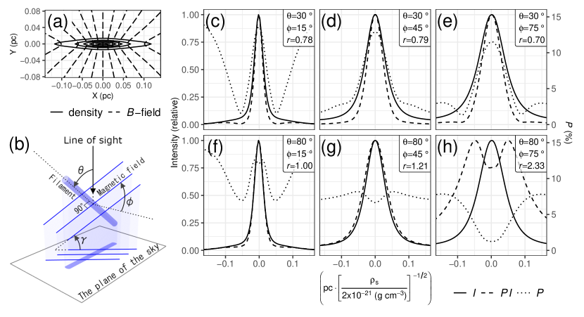
Figure 3: (a) Cross-sectional density profile of a filament perpendicular to the X–Y plane (solid contours) and its magnetic field line shapes (dashed lines), predicted by Tomisaka (2014). The density contour levels are $\rho/\rho_{c}=0.1,~{}0.3,~{}\ldots,~{}0.9$. The assumed model parameters are initial gas distribution radius $R_{0}=5$, thermal-to-magnetic pressure ratio $\beta_{0}=0.1$, and filament center-to-surface density ratio $\rho_{c}/\rho_{s}=1000$ at equilibrium (Tomisaka, 2014). (b) Definitions of the relative angle of the filament with respect to the LOS ($\theta$), relative angle of the magnetic field to the POS ($\gamma$), and the rotation angle of the magnetic field with respect to the long axis of filament ($\phi$). The origin of $\phi$ is defined as the angle when the magnetic field is on the POS. (c)–(h) Predicted profiles of I (solid line), PI (dashed line), and P (dotted line) when observing the filament shown in panel (a) from various directions of $\theta$ and $\phi$. The r in the upper right corner of each figure denotes the FWHM ratio of PI to I. We assume $2\times 10^{-21}$ (g cm^-3) as the surface density of the filament when converting the radial distribution of the gas to a physical scale in parsecs.

In Figures 3(c)–(h), we show the cross-section profiles of I and PI when we observe the model filament shown in Figure 3(a) with various orientations. To estimate the profiles, we assume a homogeneous dust alignment and dust properties in the filament. This is to demonstrate that the $\mathrm{FWHM}(\mathrm{PI})/\mathrm{FWHM}(I)$ variation can be caused solely by a pinched B-field morphology without changing the dust alignment level and dust properties. We also assume that the filament is optically thin for submillimeter radiation at 850 $\mu$m. Under these assumptions, we can estimate I and PI for each LOS looking through the filament as follows (Tomisaka, 2015):

$$I = \int\epsilon~{}\rho\left(1-P_{\mathrm{max}}\left(\frac{\cos^{2}\gamma}{2}-\frac{1}{3}\right)\right)ds,$$ (1)

$$Q = P_{\mathrm{max}}\int\epsilon~{}\rho~{}\cos 2\psi~{}\cos^{2}\gamma~{}ds,$$ (2)

$$U = P_{\mathrm{max}}\int\epsilon~{}\rho~{}\sin 2\psi~{}\cos^{2}\gamma~{}ds,$$ (3)

$$PI = \left(Q^{2}+U^{2}\right)^{1/2},$$ (4)

$$P = PI/I,$$ (5)

where the integration is performed along the LOS; $\epsilon$ is the dust emissivity; $\rho$ is the gas density; $P_{\mathrm{max}}$ is the maximum possible polarization fraction, for which we adopt a fiducial value of 0.15 (e.g., Tomisaka, 2015; King et al., 2018); $\gamma$ is the offset angle of the local B-field with respect to the POS (see Figure 3(b)); and $\psi$ is the local B-field position angle.

If the B-field is pinched in a filament, $\psi$ and $\gamma$ in Equations (1)–(4) vary spatially. The $\psi$ variation along the LOS causes geometrical depolarization. The spatial variation of this geometrical depolarization and $\gamma$ as a function of angular distance from the filament’s major axis result in different profiles of PI from that of I (Figures 3(c)–(h)). The greater the degree of B-field pinch, the more significant the difference between the two profiles.

We show in Figure 4(a) the probability distribution function (PDF) of $\mathrm{FWHM}(\mathrm{PI})/\mathrm{FWHM}(I)$ when we observe a filament with a given parameter set from random orientations in the 3D space, predicted by the Tomisaka model for typical sets of parameters. Insets in Figure 4(a) show cross-sectional views of the filament gas density and B-field structure corresponding to each parameter set. When $\rho_{c}/\rho_{s}$ is small and the B-field pinching inside the filament is negligible (e.g., the case of $\rho_{c}/\rho_{s}=10$ in the figure), the probability of the $\mathrm{FWHM}(\mathrm{PI})/\mathrm{FWHM}(I)$ ratio concentrates around 1. On the other hand, when $\rho_{c}/\rho_{s}$ becomes large, the B-field is pinched significantly toward the filament center to support the filament gas against its self-gravity (e.g., the case of $\rho_{c}/\rho_{s}=1000$ in the figure). This significant pinch of the B-field results in a significant probability of $\mathrm{FWHM}(\mathrm{PI})/\mathrm{FWHM}(I)\neq 1$, which is consistent with the observed results.

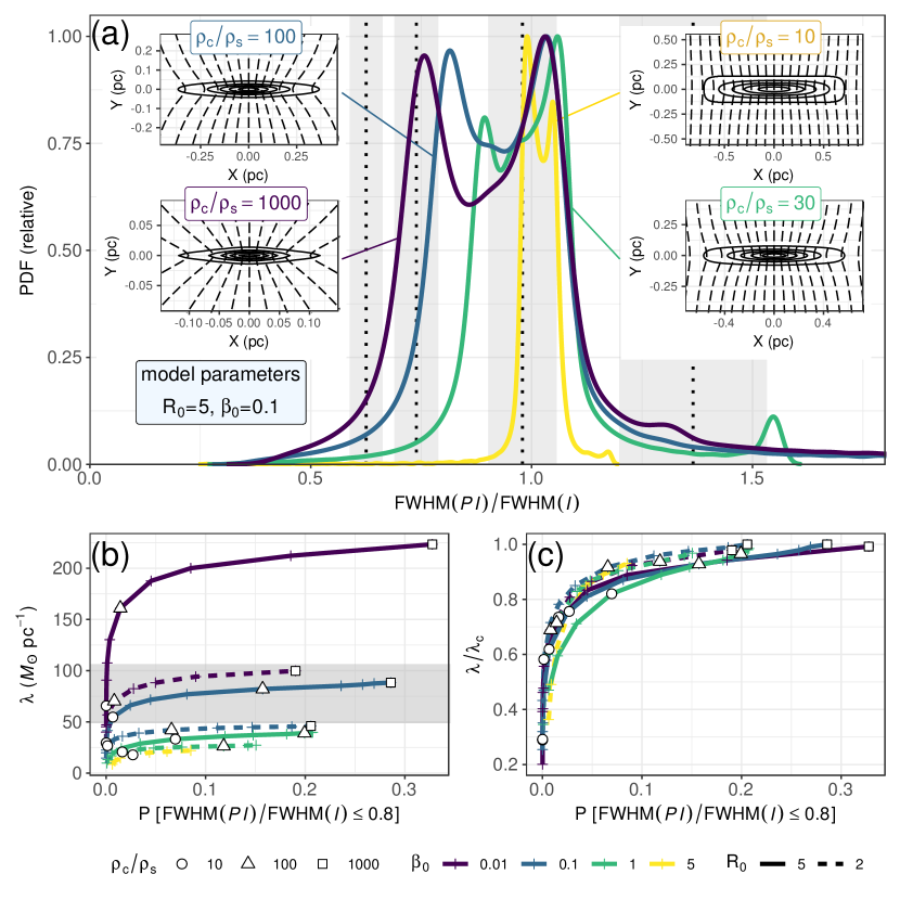
Figure 4: (a) PDF of the $\mathrm{FWHM}(\mathrm{PI})/\mathrm{FWHM}(I)$ ratio obtained for typical parameters of the model by Tomisaka (2014) when we observe the filament from a random orientation in 3D space (colored lines). We assume $R_{0}=5$, $\beta_{0}=0.1$, and $\rho_{c}/\rho_{s}=10,~{}30,~{}100,$ and 1000 in the figure. See text for the definition of $R_{0},~{}\beta_{0}$, and $\rho_{c}/\rho_{s}$. Vertical dotted lines are the observed ratios (beam-deconvolved) with their $\pm 1\sigma$ error indicated as shaded areas (segments B, A, C, and D from left to right; see Table 1). Insets show cross-sectional views of the filament gas density and B-field structure corresponding to each parameter set. Solid contours are relative density $\rho/\rho_{c}=0.1,~{}0.3,~{}\ldots,0.9$, and dashed lines represent B-field lines. We apply the same assumption as in Figures 3(c)–(h) when converting the radial distribution of the gas to a physical scale in parsecs. (b) Comparison of the filament line mass ($\lambda$) and the probability that we observe $\mathrm{FWHM}(\mathrm{PI})/\mathrm{FWHM}(I)\leqslant 0.8$ for each model parameter set. We assume a gas temperature of 15 K and a corresponding critical line mass of thermally supported filaments of $\lambda_{\mathrm{c,~{}thermal}}=2c_{s}^{2}/G\simeq 24~{}M_{\odot}~{}\mathrm{pc^{-1}}$ (Stodólkiewicz, 1963; Ostriker, 1964; Inutsuka & Miyama, 1997). The color of the lines indicates $\beta_{0}=0.01$, 0.1, 1, and 5, and the line types (solid and dashed) indicate $R_{0}=5$ and 2, respectively. Tick marks in the colored lines indicate $\rho_{c}/\rho_{s}=$2, 3, 5, 10, 20, 30, 50, 100, 200, 300, 500, and 1000. The larger $\rho_{c}/\rho_{s}$ data may not have been plotted due to numerical difficulties in obtaining equilibrium solutions at such high densities. The shaded area indicates the estimated line mass of the filament that contains regions A–D (49–106 $M_{\odot}~{}\mathrm{pc}^{-1}$; Paper I). (c) Same as panel (b) but for the ratio of $\lambda$ to the magnetically critical value ($\lambda/\lambda_{c}$).

Indeed, we find $\mathrm{FWHM}(\mathrm{PI})/\mathrm{FWHM}(I)\leqslant 0.8$ for two of the four observations (Section 3). It is difficult to reproduce $\mathrm{FWHM}(\mathrm{PI})/\mathrm{FWHM}(I)<1$ by modifying the dust alignment level, since the level needs to increase inside the dense filament to produce $\mathrm{FWHM}(\mathrm{PI})/\mathrm{FWHM}(I)<1$ (Section 3).

To verify whether the geometrical depolarization predicted by the Tomisaka model can reproduce the observation, we estimate the probability that the model predicts $\mathrm{FWHM}(\mathrm{PI})/\mathrm{FWHM}(I)\leqslant 0.8$. We plot the probability as a function of filament line mass ($\lambda$) in Figure 4(b), and $\lambda$’s ratio to the magnetically critical line mass ($\lambda/\lambda_{c}$) in Figure 4(c).

We find that the model predicts up to $\simeq 30$% probability of reproducing $\mathrm{FWHM}(\mathrm{PI})/\mathrm{FWHM}(I)\leqslant 0.8$ depending on the choice of input parameters. Paper I estimated $\lambda\sim 50$–$100~{}M_{\odot}\mathrm{pc}^{-1}$ for the filaments that contain segments A–D (shaded area in Figure 4(b)). Figure 4(b) suggests that the cases of $R_{0}=2,~{}\beta_{0}=0.01$–$0.1$ or $R_{0}=5,~{}\beta_{0}=0.1$–$1$ are preferred. In addition to that, Figure 4(c) suggests that the near-critical (or supercritical) values of $\lambda$, with $\lambda/\lambda_{\mathrm{c}}>0.9$, are preferred to reproduce the observation using the model. Since the B-field pinching depends on $\lambda/\lambda_{\mathrm{c}}$, the larger the $\lambda/\lambda_{\mathrm{c}}$, the more significant the amount of B-field pinching and, as a result, the larger the probability of $\mathrm{FWHM}(\mathrm{PI})/\mathrm{FWHM}(I)\leqslant 0.8$.

Thus, we conclude that the observed variation of the $\mathrm{FWHM}(\mathrm{PI})/\mathrm{FWHM}(I)$ ratio can be explained by pinched B-field structure inside the filament. We note that the data with $\mathrm{FWHM}(\mathrm{PI})/\mathrm{FWHM}(I)<1$ are obtained from a single filament (Figure 1). Therefore, the observed PDF may be biased toward small values of $\mathrm{FWHM}(\mathrm{PI})/\mathrm{FWHM}(I)$. We need more observations to discuss further details. At this moment, however, we can point out that the PDF estimated by the model should predict $\mathrm{FWHM}(\mathrm{PI})/\mathrm{FWHM}(I)\neq 1$ with sufficient probability. In other words, our observations strongly suggest a significant pinch of the B-field inside the filament.

5 Discussion

In the previous section, we have shown that the Tomisaka model can naturally explain the variation of observed $\mathrm{FWHM}(\mathrm{PI})/\mathrm{FWHM}(I)$ only by changing the filament’s viewing angle. It does not mean, however, that we can exclude other possibilities.

When assessing the model predictions, we assume that the dust alignment level and dust properties are homogeneous inside and outside the filament. We think it is unlikely that the dust alignment level increases at the filament center to produce $\mathrm{FWHM}(\mathrm{PI})/\mathrm{FWHM}(I)<1$ (see Section 3). On the other hand, it may be possible that the spatial variation of the dust properties causes more efficient polarization of emission at the filament center. However, in such a case, it would be necessary to explain naturally how P, which generally decreases in the molecular cloud, becomes locally higher in, e.g., segment B.

In contrast to the quiescent filament interior, the dust alignment level and dust properties may be spatially nonuniform in active regions. We show two example emission profiles at SVS 3 and SVS 13A in Figure 5 (see Appendix D for the derivation details).

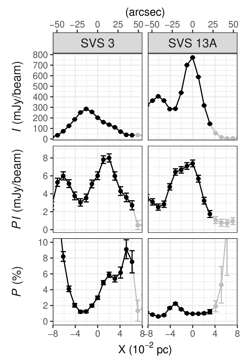
Figure 5: Same as Figure 2 but for the filaments’ cross-sectional profiles in two active regions (SVS 3 and SVS 13A).

Both the I and PI profiles show a distorted shape and do not match with each other, which is considerably different from the quiescent filaments seen in regions A–D, where a single Gaussian fits well each profile. Furthermore, the $\mathrm{PI}/\delta\mathrm{PI}$ value in these regions shows considerable spatial variation, and our criterion of achieving $\mathrm{PI}/\delta\mathrm{PI}\geqslant 3$ over more than three consecutive beams is not met. This distortion of emission profiles is potentially due to the spatial variation of the dust properties and alignment level. We limit ourselves to discussing B-field structure in quiescent filaments and do not discuss these profiles in active regions further in this paper.

The Tomisaka model assumes that an initially uniform B-field intersects a cylindrical filament perpendicularly. However, it may be possible to consider a more complex B-field. Fiege & Pudritz (2000, also see , ) showed that a helical B-field structure can reproduce observed decreases in P in dense molecular cores (“polarization holes”). We do not discuss the comparison between helical B-fields and our observations in this paper. Instead, we want to emphasize that the lateral B-field assumed in the Tomisaka model explains well the observed offset angle between the filament and the B-field (Paper I) and can also reproduce the polarization hole as demonstrated in Figure 3(h), where the B-field at the center of the filament is almost parallel to the LOS.

Disturbance of the B-field due to turbulence may be less in the center of quiescent filaments. In such a case, geometrical depolarization due to unresolved small-scale B-field turbulence may be less inside the filament than outside, resulting in a larger P and $\mathrm{FWHM}(\mathrm{PI})/\mathrm{FWHM}(I)<1$. However, if it is the primary cause of $\mathrm{FWHM}(\mathrm{PI})/\mathrm{FWHM}(I)$ variation, we need to understand why B-field turbulence is low inside one quiescent filament and high in another quiescent filament where $\mathrm{FWHM}(\mathrm{PI})/\mathrm{FWHM}(I)>1$ and the central P is small.

The variation of P inside the filament may not only be due to the geometrical effect of the pinched B-field. In fact, the observed P is $\sim 1/3$ of the model-predicted values assuming the same efficiency of polarized dust emission in the diffuse region and the filament interior (Figure 3). Thus, the efficiency of polarized dust emission may be reduced inside the filament in addition to the geometrical depolarization.

We note that the filaments in NGC 1333 may not be in exact magnetohydrostatic equilibrium, as suggested by Hacar et al. (2017). However, the equilibrium solutions of Tomisaka (2014) are probably a good representation of the structures that arise in the dynamical formation of a filament, even if equilibrium has not been achieved. In fact, Figure 4(c) indicates that the line mass may be supercritical ($\lambda/\lambda_{\mathrm{c}}>0.9$). If the filament is supercritical and the gas in the filament, which is dynamically contracting, is dragging the B-field lines toward its center, the observations should be well reproduced.

The Tomisaka model predicts a flattened filament profile, as shown in Figures 3(a) and 4(a). It results in a variation in the FWHM of the filaments’ I profiles observed from different directions, as demonstrated in Figures 3(c)–(h). This variation due to the viewing angle could be an explanation of the variance on the canonical 0.1 pc FWHM reported by, e.g., Arzoumanian et al. (2011, 2019, also see , ).

Following the discussion above, we conclude that the pinched B-field predicted by the Tomisaka model is a plausible explanation of the observed $\mathrm{FWHM}(\mathrm{PI})/\mathrm{FWHM}(I)$ variation of quiescent filaments in NGC 1333. The B-field that is dragged inward by the contracting ISM has been observed in some cases as an “hourglass” structure of the B-field around star-forming cores and is recognized as a sign of magnetically regulated collapse of spherical cores (e.g., Girart et al., 2006; Stephens et al., 2013; Kandori et al., 2017; Maury et al., 2018; Kwon et al., 2019; Hull et al., 2020). We do not see such an hourglass morphology in the observed B-field structure (Figure 1; however, see Pattle et al., 2017 for an example found in the Orion A filament). Instead, our result is an indirect observation of the possibly pinched internal B-field structure in dense interstellar filaments in star-forming regions as a result of an axisymmetrical contraction of the filament ISM. The $\mathrm{FWHM}(\mathrm{PI})/\mathrm{FWHM}(I)$ ratio, especially its deviation from 1 as we observed, may be an essential indicator of the degree of B-field pinching in filaments.

6 Conclusions

We performed submillimeter-wavelength polarization observations using SCUBA-2/POL-2 on JCMT and characterized the POS magnetic field (B-field) of NGC 1333. Following Paper I, we investigated the 3D B-field distribution inside filaments that do not show evident star-forming activity and thus are thought to retain their initial formation state. We found that the filaments’ FWHMs in PI are not the same as those in I, with two segments being appreciably narrower in PI ($\mathrm{FWHM}(\mathrm{PI})/\mathrm{FWHM}(I)\simeq 0.7$–0.8) and one segment being wider ($\mathrm{FWHM}(\mathrm{PI})/\mathrm{FWHM}(I)\simeq 1.3$) out of four investigated filament segments. None of the profiles of P inside filaments show an anticorrelation with I normally found in molecular clouds and protostellar cores.

We showed that the magnetohydrostatic equilibrium solution of a filament threaded by a lateral magnetic field (Tomisaka, 2014) well reproduces the observed variation of $\mathrm{FWHM}(\mathrm{PI})/\mathrm{FWHM}(I)$, although we do not exclude other possibilities. The B-field inside a filament is radially dragged inward (pinched) along with the matter contraction during the formation of the filament. This pinched B-field structure causes the local directional changes of the B-field within the filament and thereby the geometrical depolarization that can reproduce local variations of PI and P. The appreciable deviation of $\mathrm{FWHM}(\mathrm{PI})/\mathrm{FWHM}(I)$ from 1 indicates that the B-field is pinched significantly. In other words, quiescent filaments in NGC 1333 are suggested to be magnetically near-critical or supercritical.

The $\mathrm{FWHM}(\mathrm{PI})/\mathrm{FWHM}(I)$ ratio can provide important information about the pinched B-field structure expected inside the filament and, consequently, help us better understand the role of the B-field in the formation of filaments.

Appendix A Evaluation of Stokes Parameters and Their Sensitivity as a Function of Spatial Frequency

We estimate the Stokes I, Q, and U parameters at each position in the sky from the standard pipeline $pol2map$ (Parsons et al., 2018, software version on 2018 November 17) in Starlink (Currie et al., 2014; see Paper I for further details). As described in Paper I, we apply a 2D least-squares fit of a second-order polynomial using a Gaussian kernel to the Stokes I, Q, and U data. We debias PI to correct a possible offset due to the square-sum of the Q and U errors. We then use only $\mathrm{PI}/\delta\mathrm{PI}\geqslant 3$ data for the following analyses to make the debiasing effect negligible. The assumed FWHM of the Gaussian kernel is $14\arcsec.1$, which corresponds to the JCMT/POL-2 beam at $850~{}\mu$m if we fit the beam with a single Gaussian profile (Dempsey et al., 2013).

The Stokes I intensity is estimated by removing background atmospheric emission from the observed data, resulting in a reduced sensitivity for the large-scale emission. On the other hand, Q and U are measured in AC mode performed while rotating a half-wave plat; thus, the sensitivity is retained for the large-scale emission. We estimate the spatial power spectra of these emissions and PI along the blue dashed line in Figure 1 to test if the sensitivities of I, Q, and U are consistent for the small-scale emission, which is the subject of this paper. As shown in Figure A.1 (top panel), the spectral shapes are consistent with each other. Also, we find the nearly constant PI/I ratio of spectral amplitude, as shown in Figure A.1 (bottom panel). Thus, we confirm that the sensitivities of I and PI are consistent for the small-scale $(\leqslant 2\arcmin)$ structures.

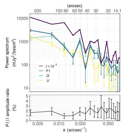
Figure A.1: Top panel: spatial power spectra of I, Q, U, and PI signals measured along the blue dashed line in Figures 1 and A.3. Bottom panel: ratio between PI and I spectrum amplitudes.

Appendix B Evaluation of Filaments’ Cross-sectional Profiles

We select the data with $\mathrm{PI}/\delta\mathrm{PI}\geqslant 5$ for segments A, B, and C and $\mathrm{PI}/\delta\mathrm{PI}\geqslant 3$ for segment D and estimate the position angles of the major axes of the filaments at each position. By assuming that we can approximate filaments locally by straight lines, we estimate the position angles by least-squares linear fits to the spatial structures in I, weighted by I intensity. The estimated position angles are listed in Table A.1, together with those of active regions described in Appendix D. We then set the FWHM of the Gaussian kernel as $14\arcsec.1$ in the direction perpendicular to the filament and $70\arcsec.5$, or five times the beam, in the direction along the filament and reestimate the Stokes I, Q, and U parameters at each position in the sky to estimate the cross-sectional profiles of filaments with improved S/Ns. We show the estimated Stokes I maps and the PI maps, which are estimated from the Stokes Q and U maps in Figure A.2, together with the assumed beam profile.

Table A.1: Estimated Position Angles of the Filaments

Segment	Position Angle
	(deg)
A	$-20.9\pm 11.6$
B	$-7.8\pm\ \,4.4$
C	$-14.4\pm\ \,3.7$
D	$12.5\pm 12.9$
SVS 3	$-35.9\pm\ \,1.8$
SVS 13A	$-47.1\pm\ \,3.5$
Note. See text for the details of the derivation.

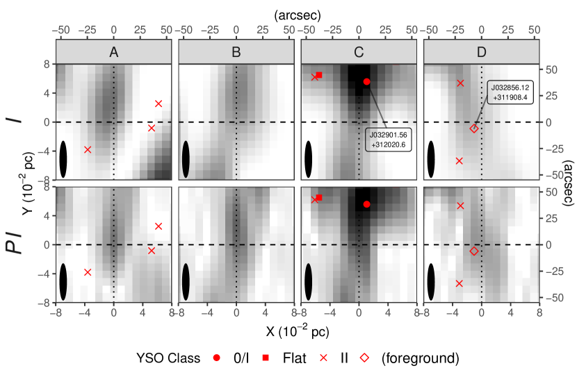
Figure A.2: Spatially smoothed distribution of $850~{}\mu\mathrm{m}$ Stokes $I$ and polarized emission $PI$ of the four selected regions. The positions of the regions are indicted in Figure 1. We assume $14\arcsec.1$ spatial resolution (FWHM) across the filament direction and $70\arcsec.5$ in the filament direction, to achieve good SNRs in the cross-sectional profiles of filaments. YSOs found near the positions of cross-sections (Evans et al., 2009; Young et al., 2015) are marked with red symbols. We set the position of segment C so that we can exclude one Class 0/I YSO (J032901.56+312020.6) from the evaluation of the cross-section (Section 2). We ignore one Class II YSO (J032856.12+311908.4) in region D as a foreground source since the estimated $A_{V}=0$ mag (Evans et al., 2009). The assumed Gaussian beams are indicated in the bottom left corners of the figures.

We estimate errors by performing a Monte Carlo simulation by assuming a Gaussian distribution for the pol2map-estimated error. We repeat the polynomial fitting 1000 times with Gaussian random errors at each position. We take the mean of 1000 samples as the estimated values and the standard deviation as the estimation error of each position.

We fit the estimated cross-sectional profiles of I and PI with Gaussian curves as shown in Figure 2. We use the data that satisfy both $I/\delta I\geqslant 3$ and $\mathrm{PI}/\delta\mathrm{PI}\geqslant 3$ for fitting I and PI profiles. Practically, all data points with $\mathrm{PI}/\delta\mathrm{PI}\geqslant 3$ satisfy $I/\delta I\geqslant 3$. When making Gaussian fittings, we assume the baseline intensity of I and PI as zero and judge the residual low S/N signal seen in PI (Figure 2) as residual noise of the debiasing. If we estimate the Gaussian baseline level with these signals, positive baseline levels lead to narrow PI profiles.

We then deconvolve the fitted Gaussian by the observational beam by assuming the beam as a $14.\arcsec 1$ single Gaussian (Dempsey et al., 2013) as follows:

$$\sigma_{\mathrm{deconvolved}}=\sqrt{\sigma_{\mathrm{observed}}^{2}-\sigma_{\mathrm{beam}}^{2}},$$ (B1)

where $\sigma_{\mathrm{deconvolved}}$, $\sigma_{\mathrm{observed}}$, and $\sigma_{\mathrm{beam}}$ are the variances of deconvolved, observed, and the beam’s Gaussian, respectively.

Appendix C Dust Temperature

We refer to Pezzuto et al. (2021, Figure A.3) and estimate the dust color temperature at the filament profiles. We confirm that there are no significant heating sources embedded in the regions, and there is no significant nonuniform external heating from nearby sources. The estimated dust temperature at each profile is $T=12.2$–15.8 K for region A, 12.6–16.0 K for region B, 13.1–17.0 K for region C, and 12.9–13.7 K for region D.

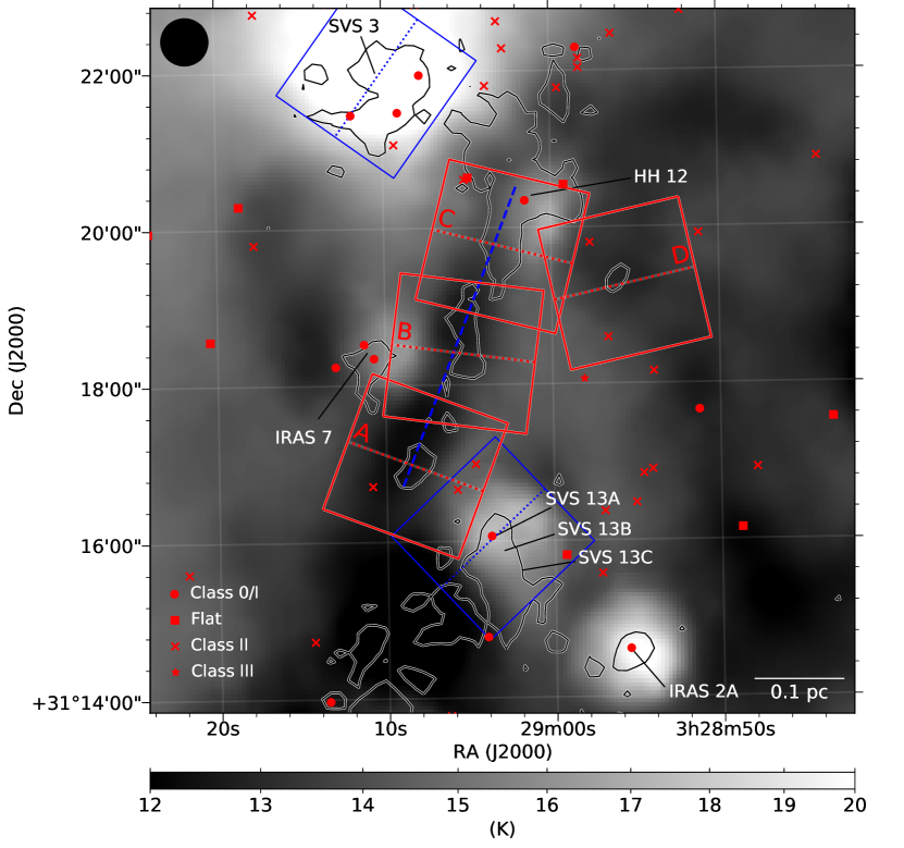
Figure A.3: Same as Figure 1 but for dust color temperature estimated by Herschel and Planck observations (Pezzuto et al., 2021). The resolution of the map ($36\arcsec.1$) is shown in the upper left corner of the figure.

Appendix D Filament Profiles in Active Regions

We estimate two example cross-sectional profiles of filaments in the active region. We set the positions at SVS 3 and SVS 13A, as shown in Figures 1 and A.3. For these regions, we select the data with $I\geqslant 25$ (mJy beam^-1) and estimate the local filament position angles as described in Appendix B. We do not restrict the data based on $\mathrm{PI}/\delta\mathrm{PI}$ to estimate the filament’s position angles, as the S/N of PI largely fluctuates in the active regions. The estimated position angles are shown in Table A.1. We then estimate I and PI intensity maps smoothed along the major axes of the filaments as described in Appendix B. The estimated intensity maps are shown in Figure A.4. The cross-sectional profiles of I, PI, and P are shown in Figure 5.

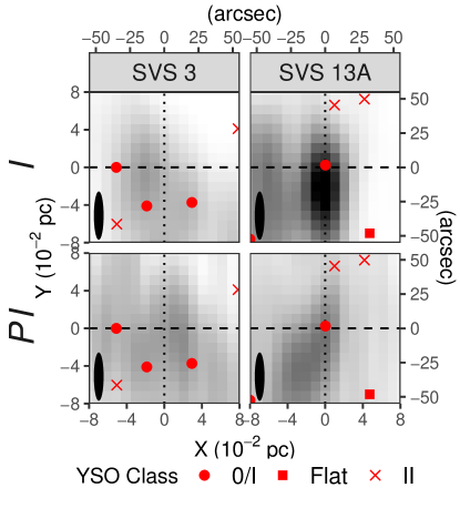
Figure A.4: Same as Figure A.2 but for maps of two active regions. The two regions are centered at SVS 3 and SVS 13A.

References

- André et al. (2014) André, P., Di Francesco, J., Ward-Thompson, D., et al. 2014, Protostars and Planets VI, 27, doi: 10.2458/azu_uapress_9780816531240-ch002
- Arzoumanian et al. (2011) Arzoumanian, D., André, P., Didelon, P., et al. 2011, A&A, 529, L6, doi: 10.1051/0004-6361/201116596
- Arzoumanian et al. (2019) Arzoumanian, D., André, P., Könyves, V., et al. 2019, A&A, 621, A42, doi: 10.1051/0004-6361/201832725
- Arzoumanian et al. (2021) Arzoumanian, D., Furuya, R. S., Hasegawa, T., et al. 2021, A&A, 647, A78, doi: 10.1051/0004-6361/202038624
- Astropy Collaboration et al. (2013) Astropy Collaboration, Robitaille, T. P., Tollerud, E. J., et al. 2013, A&A, 558, A33, doi: 10.1051/0004-6361/201322068
- Auddy et al. (2016) Auddy, S., Basu, S., & Kudoh, T. 2016, ApJ, 831, 46, doi: 10.3847/0004-637X/831/1/46
- Bino & Basu (2021) Bino, G., & Basu, S. 2021, ApJ, 911, 15, doi: 10.3847/1538-4357/abe6a4
- Currie et al. (2014) Currie, M. J., Berry, D. S., Jenness, T., et al. 2014, in Astronomical Society of the Pacific Conference Series, Vol. 485, Astronomical Data Analysis Software and Systems XXIII, ed. N. Manset & P. Forshay, 391
- Dempsey et al. (2013) Dempsey, J. T., Friberg, P., Jenness, T., et al. 2013, MNRAS, 430, 2534, doi: 10.1093/mnras/stt090
- Dionatos et al. (2020) Dionatos, O., Kristensen, L. E., Tafalla, M., Güdel, M., & Persson, M. 2020, A&A, 641, A36, doi: 10.1051/0004-6361/202037684
- Doi et al. (2020) Doi, Y., Hasegawa, T., Furuya, R. S., et al. 2020, ApJ, 899, 28, doi: 10.3847/1538-4357/aba1e2
- Evans et al. (2009) Evans, II, N. J., Dunham, M. M., Jørgensen, J. K., et al. 2009, ApJS, 181, 321, doi: 10.1088/0067-0049/181/2/321
- Fiege & Pudritz (2000) Fiege, J. D., & Pudritz, R. E. 2000, ApJ, 544, 830, doi: 10.1086/317228
- France et al. (2014) France, K., Schindhelm, R., Bergin, E. A., Roueff, E., & Abgrall, H. 2014, ApJ, 784, 127, doi: 10.1088/0004-637X/784/2/127
- Girart et al. (2006) Girart, J. M., Rao, R., & Marrone, D. P. 2006, Science, 313, 812, doi: 10.1126/science.1129093
- Hacar et al. (2017) Hacar, A., Tafalla, M., & Alves, J. 2017, A&A, 606, A123, doi: 10.1051/0004-6361/201630348
- Hennebelle & Inutsuka (2019) Hennebelle, P., & Inutsuka, S.-i. 2019, Frontiers in Astronomy and Space Sciences, 6, 5, doi: 10.3389/fspas.2019.00005
- Hildebrand (1988) Hildebrand, R. H. 1988, QJRAS, 29, 327
- Hoang et al. (2021) Hoang, T., Tram, L. N., Lee, H., Diep, P. N., & Ngoc, N. B. 2021, ApJ, 908, 218, doi: 10.3847/1538-4357/abd54f
- Hull et al. (2020) Hull, C. L. H., Le Gouellec, V. J. M., Girart, J. M., Tobin, J. J., & Bourke, T. L. 2020, ApJ, 892, 152, doi: 10.3847/1538-4357/ab5809
- Inutsuka & Miyama (1997) Inutsuka, S.-i., & Miyama, S. M. 1997, ApJ, 480, 681, doi: 10.1086/303982
- Kandori et al. (2017) Kandori, R., Tamura, M., Tomisaka, K., et al. 2017, ApJ, 848, 110, doi: 10.3847/1538-4357/aa8d18
- Kashiwagi & Tomisaka (2021) Kashiwagi, R., & Tomisaka, K. 2021, ApJ, 911, 106, doi: 10.3847/1538-4357/abea7a
- King et al. (2018) King, P. K., Fissel, L. M., Chen, C.-Y., & Li, Z.-Y. 2018, MNRAS, 474, 5122, doi: 10.1093/mnras/stx3096
- Kwon et al. (2019) Kwon, W., Stephens, I. W., Tobin, J. J., et al. 2019, ApJ, 879, 25, doi: 10.3847/1538-4357/ab24c8
- Lazarian & Hoang (2007) Lazarian, A., & Hoang, T. 2007, MNRAS, 378, 910, doi: 10.1111/j.1365-2966.2007.11817.x
- Maury et al. (2018) Maury, A. J., Girart, J. M., Zhang, Q., et al. 2018, MNRAS, 477, 2760, doi: 10.1093/mnras/sty574
- Ortiz-León et al. (2018) Ortiz-León, G. N., Loinard, L., Dzib, S. A., et al. 2018, ApJ, 865, 73, doi: 10.3847/1538-4357/aada49
- Ostriker (1964) Ostriker, J. 1964, ApJ, 140, 1056, doi: 10.1086/148005
- Parsons et al. (2018) Parsons, H. A. L., Berry, D. S., Rawlings, M. G., & Graves, S. F. 2018, The POL-2 Data Reduction Cookbook, 1st edn., Starlink Project, East Asian Observatory
- Pattle et al. (2017) Pattle, K., Ward-Thompson, D., Berry, D., et al. 2017, ApJ, 846, 122, doi: 10.3847/1538-4357/aa80e5
- Pezzuto et al. (2021) Pezzuto, S., Benedettini, M., Di Francesco, J., et al. 2021, A&A, 645, A55, doi: 10.1051/0004-6361/201936534
- Reissl et al. (2018) Reissl, S., Stutz, A. M., Brauer, R., et al. 2018, MNRAS, 481, 2507, doi: 10.1093/mnras/sty2415
- Sandell & Knee (2001) Sandell, G., & Knee, L. B. G. 2001, ApJ, 546, L49, doi: 10.1086/318060
- Stein (1966) Stein, W. 1966, ApJ, 144, 318, doi: 10.1086/148606
- Stephens et al. (2013) Stephens, I. W., Looney, L. W., Kwon, W., et al. 2013, ApJ, 769, L15, doi: 10.1088/2041-8205/769/1/L15
- Stodólkiewicz (1963) Stodólkiewicz, J. S. 1963, Acta Astron., 13, 30
- Tomisaka (2014) Tomisaka, K. 2014, ApJ, 785, 24, doi: 10.1088/0004-637X/785/1/24
- Tomisaka (2015) —. 2015, ApJ, 807, 47, doi: 10.1088/0004-637X/807/1/47
- Tomisaka (2021) —. 2021, ApJ, 920, 161, doi: 10.3847/1538-4357/ac295a
- Young et al. (2015) Young, K. E., Young, C. H., Lai, S.-P., Dunham, M. M., & Evans, II, N. J. 2015, AJ, 150, 40, doi: 10.1088/0004-6256/150/2/40
- Zucker et al. (2018) Zucker, C., Schlafly, E. F., Speagle, J. S., et al. 2018, ApJ, 869, 83, doi: 10.3847/1538-4357/aae97c
- Zucker et al. (2019) Zucker, C., Speagle, J. S., Schlafly, E. F., et al. 2019, ApJ, 879, 125, doi: 10.3847/1538-4357/ab2388